Center for Demography and Ecology
University of Wisconsin-Madison
Social Class Indicators and Health at Midlife
Richard A. Miech
Robert M. Hauser
CDE Working Paper No. 98-06
1 Prepared for the Meetings of the Population Association of America, Chicago, Illinois, April1998. Support for this research was provided by the National Institute on Aging (AG-9775), theNational Science Foundation (SBR-9320660), the Vilas Estate Trust, and the Center forDemography and Ecology at the University of Wisconsin-Madison. We thank John RobertWarren for preparing socioeconomic measures for occupations in the 1970 Census. The opinionsexpressed herein are those of the authors. Data and documentation from the WisconsinLongitudinal Study are available at http://dpls.dacc.wisc.edu/WLS. Data extracts and summarystatistics used in this analysis are available from the authors. Address correspondence to RobertM. Hauser, Department of Sociology, The University of Wisconsin-Madison, 1180 ObservatoryDrive, Madison, Wisconsin 53706, or E-Mail to [email protected].
Social Class Indicators and Health at Midlife1
Richard A. MiechRobert M. Hauser
Department of SociologyCenter for Demography and EcologyThe University of Wisconsin-Madison
March 1998
Social Class Indicators and Health at Midlife
Abstract
There are several competing schemes for the measurement of social and economic
standing in studies of health and well-being. We address the predictive validity of several
alternative measures of social class and socioeconomic standing in relation to an array of health
outcomes in the Wisconsin Longitudinal Study. The WLS has successfully followed a large
cohort of Wisconsin high school graduates from 1957 to 1992-93, when they were 53 or 54 years
old. We find that occupational education has modest relationships with self-reported general
health and that it dominates other occupation-based measures, at least among men. Social class,
as specified by Wright or by Erikson and Golthorpe, bears little relation to this health measure.
None of the occupation-based measures adds to the effects on self-reported general health of
either educational attainment or the combination of education with personal income.

Within the past few years, there has been renewed interest in socioeconomic status and its
relationship with health and well-being (Kaplan and Lynch 1997; Moss 1997; Krieger, et al.
1997). Sources of this interest probably include rising economic inequality in the United States
and demands for improved social reporting of SES-health relationships, along with evidence of
the persistence or growth of differential health outcomes (Marmot, et al. 1997). Prompted by
these developments, we have investigated the measurement of occupational standing and social
class in studies of health and well-being. Specifically, we have used a unique set of data on
Wisconsin high school graduates at midlife to compare the relationships between several
alternative measures of occupational standing or social class and a widely-used item on self-
reported health. Our goal is to help specify the most appropriate measures of socioeconomic
status to use in studying differentials in health.
The plan of the paper is as follows. We briefly review commonly used socioeconomic
measures, focusing on occupation-related measures including prestige, socioeconomic status, and
social class. Then, we consider alternative measures of health and well-being. While there are
numerous possibilities, we focus here on a single measure, self-reported general health. We
estimate the overall relationships between that health measure and several occupation-based
measures in the Wisconsin Longitudinal Study (WLS). The WLS has both strengths and
weaknesses for a study of this kind, and we review them before continuing with the analysis.
Next, we ask whether one occupational standing or social class variable dominates the others.
That is, we ask whether each measure adds anything to predictions of the general health item
when the others are controlled. Last, we ask whether any of the occupation or social class
measures adds to predictions of the general health item when educational attainment or personal
income has been controlled.

2 Whether socioeconomic status is merely a convenient shorthand expression for variableslike these, or whether such variables, taken collectively, behave as if they formed a unitaryconstruct is a matter of continuing study and discussion.
2
Socioeconomic Concepts and Measures in Health Research
Socioeconomic status is typically used as a shorthand expression for variables that
characterize the placement of persons, families, households, census tracts, or other aggregates
with respect to the capacity to create or consume goods that are valued in our society. Thus,
socioeconomic status may be indicated by educational attainment, by occupational standing, by
social class, by income (or poverty), by wealth, by tangible possessions—such as home appliances
or libraries, houses, cars, boats, or by degrees from elite colleges and universities. At some times,
it has also been taken to include measures of participation in social, cultural, or political life.2
In sociological and epidemiological studies of health and well-being, socioeconomic status
is usually represented by one or more of (a) educational attainment, (b) economic resources,
typically measured by annual income, and (c) occupational status or prestige. Studies often
employ only one of these three SES variables. This procedure rests on two implicit assumptions:
All three measures index the same underlying property, and none carries much information,
independent of the others. However, while there are substantial correlations among education,
occupation, and income, it is well established that each also has unique antecedents and
consequences (Sewell and Hauser 1975). Thus, each variable has different theoretical properties
and may have unique strengths and weaknesses for investigations of health outcomes. In this
context, a key issue is variation in the causal relationship between health and SES: Does
socioeconomic status affect health? Or does health affect socioeconomic status? Or are observed

3
relationships between socioeconomic status and health brought about by other, possibly
unobserved variables?
The strengths of education as a socioeconomic measure include the fact that it is easy to
measure in social surveys and that it applies to people who are not in the labor force. In addition,
health problems in middle and late adulthood cannot affect years of education, which are typically
completed early in the life course. Thus, excepting the possibility of common causation,
associations between education and adult health outcomes represent effects of SES on adult
health, and not vice-versa. Clear, unidirectional interpretations of SES/health associations are
usually not possible with income and occupational status measures, which may be negatively
affected by impaired health, and thus reflect reciprocal causation.
At the same time, educational attainment has two potential disadvantages as an indicator
of socioeconomic status in studies of health and well-being. First, its imperviousness to health
problems in middle and late adulthood may also serve as a disadvantage if the research question
under investigation concerns the effects of adult health changes on SES. Second, educational
levels may have different meanings across historical time, especially in light of the vast increase in
educational attainment across cohorts in the 20th century (National Center for Education Statistics
1995). In short, a college degree was much rarer and, consequently, signified relatively higher
status 50 years ago than it does today, and may have different health consequences. Analyses
based on cross-sections of the population that include a wide range of ages, therefore, should
consider the potentially different health “returns” on education across birth cohorts. This

3 Moreover, the validity of this relative interpretation of educational attainment is open toquestion.
4
potential bias, however, does not affect analyses that are based on a single birth cohort, such as
the present study.3
The second socioeconomic indicator, income from work, may and often does vary greatly
from year to year, and thus it may be affected by health changes in middle and late adulthood.
Indeed, recent economic analyses suggests that a large part of the association between income and
health problems in late adulthood results from effects of health on income (Smith and Kington
1997a; Smith and Kington 1997b). Three characteristics of income affect its use in studies of
SES and health. First, survey members are often reluctant to provide information on their
income, and many refuse outright to disclose this information; even willing respondents often do
not know or neglect to report some components of their incomes. Second, the relationship
between income and health does not appear to be linear, as small changes in income are associated
with much larger changes in health among poor as compared to wealthy families (Backlund, et al.
1996; Kitagawa and Hauser 1973). Finally, the association between income and health outcomes
represents both the effect of income on health and the effects of health on income, which
introduces difficulties both in estimating and interpreting the income-health relationship.
The third socioeconomic measure is occupational standing, which is either employed in
research as a distinct indicator or else combined with other information to form an omnibus
measure of social class. Like income, occupation may be both cause and consequence of health
and well-being. Unlike income, survey respondents rarely refuse to report or describe their
occupations, and retrospective data on occupations are not markedly poorer in quality than

4 To be sure, there are alternative ways of reporting educational attainment, e.g., in yearsof school attended or completed or in terms of educational credentials. Likewise, income reportsand the properties of those reports vary with the choice of sources and reporting periods, andsome studies attempt to specify permanent income or wealth. Moreover, income is sometimesspecified relative to “needs,” where the latter variable is determined by the official poverty level.
5 Hauser and Warren (1997) have reviewed measures of occupational standing based onthe U.S. Census classifications of occupation and industry from 1950 through 1990.
6 However, there is reason to believe that the Nakao-Treas index will behave similarly tothe Duncan SEI or to occupational education (Warren, et al. forthcoming).
5
contemporaneous data. However, detailed collection and classification of occupational data is
time-consuming and expensive (Hauser and Warren 1997).
Unlike educational attainment and income, which are usually conceptualized in a
straightforward manner,4 a proliferation of alternative occupational and class measures has been
used in sociological and epidemiological research. Measures evaluated in this study that are based
solely on a subject’s occupation are the occupational prestige scales developed by Siegel (1971),
the Duncan SEI - socioeconomic index for occupations (Duncan 1961), Blau and Duncan’s
(1967) 17-category classification of occupation, industry, and class-of-worker (Group II), and
recent measures of occupational education and occupational income developed by Hauser and
Warren (1997).5 Social class measures that we evaluate in this study include Erik Olin Wright’s
measure of social class (Wright 1997), as well as Robert Erikson and John Goldthorpe’s social
class schema (Erikson and Goldthorpe 1992).
The foregoing are not the only occupational and social class measures that are currently
used in research, although they are some of the more popular ones. Other occupational measures
not evaluated in this study include the British Registrar General’s Scale (Marmot, et al. 1987),
Nakao and Treas’ measure of occupational socioeconomic status (Nakao and Treas 1994),6 the
7 However, one recent effort is Gregorio, Walsh, and Paturzo (1997).
6
Hollingshead Index of Social Position (Hollingshead 1957), the Nam-Powers socioeconomic
status scores (Nam and Powers 1983), and the Warner index of status characteristics (Miller
1991).
In general, occupation-based measures have two primary disadvantages that we address in
this study. First, the wide array of measures available is somewhat bewildering, and few studies
have compared and contrasted their potentially different relations to health (see Liberatos, Link,
and Kelsey (1988) for an exception). Few studies compare the relationship of the same health
measure to different occupational measures within a single body of data,7 and effects of various
occupational measures are difficult to compare across studies that employ different samples and
address different health outcomes. As a result, the extent to which different occupation-based
status measures influence study conclusions is unknown. Researchers deciding between
alternative measures to include in their surveys are often forced to rely on intuition, convenience,
or tradition, rather than scientific evidence. In this study we take initial steps to document
differences between occupation-based SES measures by directly comparing several occupational
indicators in relation to the same health outcome.
A second, related, issue concerns the overall utility of occupation-based SES measures in
studies of health and can be summarized by the question: do occupational measures contribute any
information above and beyond measures of individual education and income? This question takes
on particular importance considering that occupational measures are often expensive to include in
health surveys because they require several questions, and the responses must be coded by trained
personnel. The issue of whether occupational measures warrant the time and money they require
8 However, the Duncan SEI, which has gained wide use in studies of social mobility, wasoriginally developed for use in mortality analysis.
9 For a similar proposal, see Krieger and Fee (1994). One of Krieger, Williams, andMoss’s contributions is to suggest socioeconomic measures at the neighborhood level, as well asfor individuals and households, but their proposed measure of neighborhood social class is simplyan aggregate of employment in eight Census major occupation groups, which has no clearconnection with Wright’s class concept (1997:355).
7
is further highlighted by the fact that most occupational measures were not specifically designed
for health studies,8 but, rather, were developed by government agencies or by sociologists with a
more general interest in social stratification. The association of occupational measures with
health, net of individual education and income, remains an open question because it was not
assessed during the development of most occupational measures, and has not been examined in
detail.
Wright’s (1997) measure of social class is a particularly noteworthy example of an
occupational measure that warrants more empirical investigation. Wright’s index is rigorously
derived from Marxist theory and consists of 12 categories, such as “capitalist” and “non-skilled
workers,” that seem intuitively plausible as a powerful classification of class structure. In fact, in
their recent review article, Krieger, Williams and Moss (1997) suggest that U.S. Vital Statistics
should incorporate a measure of social class, and highlight Wright’s measure as a candidate index.
However, their recommendation comes despite the fact that almost nothing is known about the
measure’s association with health or well-being.9 While the theoretical clarity of the Wright
measure is certainly appealing, research is needed to determine the utility of this measure. That is,
we need to estimate the relationship of Wright’s measure with health and well-being and, also, to
determine whether it contributes any more to our understanding of health than simpler measures

8
of income, education, or occupation. While we know of no specific claims on behalf of the
Erikson-Goldthorpe class scheme in health research, its frequent use as an alternative to Wright’s
class scheme suggests the value of evaluating its validity in the same way.
The Wisconsin Longitudinal Study
The data for this investigation come from the Wisconsin Longitudinal Study (WLS),
which is based on a random sample of 10,317 men and women who graduated from Wisconsin
high schools in 1957. Almost all sample members were born in 1939. The survey has collected
data from the original respondents in 1964, 1975, and 1992-93 (Sewell and Hauser 1992). The
analysis in this study is based on the 1992-93 wave of data collection, which includes 8,500
telephone interviews of 9,750 surviving men and women and a subset of approximately 6,900 men
and women who completed a mail survey that included a section on health outcomes. Most
respondents were 53 or 54 years old during the last wave of data collection.
In the 1992-93 WLS surveys, we updated our measurements of marital status, child-
rearing, education, labor force participation, jobs and occupations, social participation, and future
aspirations and plans among the Wisconsin graduates (Hauser, et al. 1992; Hauser, et al. 1994).
In addition, we expanded the content of earlier follow-ups to include psychological well-being,
mental and physical health, wealth, household economic transfers, and social comparison and
exchange relationships with parents, siblings, and children. We weighed our previous concepts
and methods, which resemble those of the Current Population Survey (CPS) and the 1973
Occupational Changes in a Generation Survey (OCG), against comparability with other well-
designed surveys, e.g., the Health and Retirement Survey (HRS), the National Survey of Families
and Households (NSFH), NIH surveys of work and psychological functioning, and the NORC
10 There have, of course, been important and influential longer-term studies of the life-course in the U.S. These reflect careful and insightful work, but they are based on small, local, orhighly selected samples (Terman and Oden 1959; Elder 1974; Clausen 1993).
9
General Social Survey (GSS). We also coordinated our design with members of the MacArthur
Foundation Research Network on Successful Midlife Development, with the Whitehall II study
(Marmot, et al. 1991), and with M.E.J. Wadsworth's (1991) longitudinal study of persons born in
Great Britain in 1946.
Among Americans aged 50 to 54 in 1990 and 1991, approximately 66 percent are non-
Hispanic white women and men who completed at least 12 years of schooling (Kominski and
Adams 1992) and thus resemble the WLS cohort. The WLS cohort precedes by about a decade
the bulk of the baby boom generation that continues to tax social institutions and resources at
each stage of life. For this reason, the study can provide early indications of trends and problems
that will become important as the larger group passes through its fifties. In addition, the WLS is
the first of the large, longitudinal studies of American adolescents, and it thus provides the first
large-scale opportunity to study the life course from late adolescence through the mid-50s in the
context of a full record of ability, aspiration, and achievement.10
The WLS data also have obvious limitations. Some strata of American society are not
represented. Everyone in the primary sample graduated from high school. Sewell and Hauser
(1975:207-15) estimated that about 75 percent of Wisconsin youth graduated from high schools
in the late 1950s. There are only a handful of African American, Hispanic, or Asian persons in the
WLS. Given the minuscule share of minorities in Wisconsin when the WLS began, there is no
way to remedy this omission. About 19 percent of the WLS sample is of farm origin; this is
consistent with national estimates in cohorts of the late 1930s. In 1964, in 1975, and again in

10
1992, 70 percent of the sample lived in Wisconsin, but 30 percent lived elsewhere in the U.S. or
abroad.
The WLS has both strengths and weaknesses as a vehicle for studies of socioeconomic
differentials in health. Its strengths include a large sample size, coverage of both women and men,
and careful measurement of several relevant socioeconomic constructs. Moreover, the age of the
sample is appropriate, for prior studies have found that socioeconomic differentials in health
become more pronounced at midlife (House, et al. 1990; House, et al. 1994). Weaknesses of the
WLS include the restriction of the sample to high school graduates, the omission of minorities,
and the limited regional origin of the sample. We would especially discourage any generalization
of the present findings to persons with less than a high school diploma or to minority populations.
Measures of Occupational Standing and Social Class
Descriptive statistics of the occupational standing measures examined in this study appear
in Table 1, and are based on the 1970 Census Occupational Classification. The first measure we
examine is occupational prestige (Siegel 1971). Prestige is a concept that may measure either a
relationship of deference or derogation between role incumbents, or the general desirability or
goodness of an occupation. Siegel’s prestige measures for 1970 Census occupation categories
are based on a series of surveys carried out by the National Opinion Research Center in the mid-
1960s. Survey respondents were asked to rate occupation titles on a nine-point scale of general
social standing. While the exact theoretical meaning of the prestige concept is debated heatedly in
the sociological literature, there is consensus that it is a statistically robust measure. Prestige
ratings show little variation regardless of how people are asked to rate occupations (Kraus, et al.
1978), whether occupations are rated by men or women (Bose and Rossi 1983), the race of raters

11 The Census characteristics were age-standardized, but that had little influence on thefindings.
12 For further discussion of this point, see Hauser and Warren (1997:190-198).
13 There are minor errors in the Duncan SEI scores reported by Hauser and Featherman(1977:319-329), and a corrected listing is available from the authors.
11
(Siegel 1970), the historical period in which ratings were obtained (Hodge, et al. 1964; Nakao and
Treas 1994; Hauser 1982), or raters’ location in the social hierarchy within industrialized nations
and most of the non-industrialized world (Treiman 1977; Haller and Bills 1979).
The second occupational measure we investigate is the Duncan socioeconomic index
(SEI) of occupations (Duncan 1961), a measure that was originally developed as a proxy for
occupational prestige. Early prestige surveys did not include a comprehensive list of occupation
titles, and the procedure Duncan used to impute scores for unrated occupations is the model for
later socioeconomic indexes. In brief, for 45 occupations rated in a 1947 NORC prestige survey,
which could be matched to titles in the 1950 Census, Duncan took the percentages of “good” or
“excellent” ratings that they received on a five-point scale and regressed them on the two factors
of (a) occupational education, as measured by the percentage of male occupational incumbents
who had completed high school or more and (b) occupational income, as measured by the
percentage of male incumbents who reported incomes of $3500 or more in 1949.11 The estimated
regression coefficients from this analysis were used to compute socioeconomic scores for all
occupations. That is, the Duncan SEI is a weighted index of the occupational education and
occupational income of men in the 1950 Census; it is not a measure of occupational prestige.12
In the present study we use an update of the Duncan index for 1970 Census occupational
titles (Hauser and Featherman 1977).13 In general, prestige and SEI measures are highly

14 We thank John Robert Warren for extracting these occupational characteristics from aspecial tabulation of 1970 Census data, which was originally prepared for Charles Nam and MaryPowers. The data are available from the authors.
12
ln(yi%1
100&yi%1)
correlated, but the higher criterion validity of the Duncan SEI (and similar measures) has led to
their greater acceptance and use in the sociological literature (Featherman and Hauser 1976;
Hauser and Warren 1997; Warren, et al. forthcoming).
The final two scalar measures of occupational standing we examine in this study are
occupational education and occupational income, which correspond to the two components of the
Duncan SEI. Recent analyses of socioeconomic mobility support the surprising conclusion that
occupational education alone serves as a more powerful indicator of socioeconomic standing than
occupational income, occupational prestige, or occupational SEI (Hauser and Warren 1997;
Hauser 1998). In this study we ask whether this same finding holds in analyses of health. Hauser
and Warren (1997) used occupational data from the 1990 Census, but because occupational data
in the WLS are currently available in the 1970 Census classification, we used corresponding data
from the 1970 Census. Occupational education is the percentage of an occupation’s incumbents
who had one or more years of college education in the 1970 census, and occupational income is
the percentage of an occupation’s incumbents who earned $10,000 or more in the year preceding
the 1970 census.14 Following Hauser and Warren (1997:204), we re-expressed each percentage
using a started logit transformation:
where yi is the percentage of workers above the threshold.

15 There are actually two differences between the health subsample and all graduaterespondents: response to the health survey and availability of complete information for all of theoccupation or class measures.
13
Table 2 gives the Group II occupation distributions of the WLS sample by sex and by
completion of the health mailback survey. These show the expected high concentration of male
and female WLS graduates in professional and salaried managerial occupations, as well as a
concentration of female graduates in clerical work.
Note that, in Table 1, each measure of occupational standing has a slightly higher mean
among respondents to the health mailback survey than among all telephone respondents. Also, in
Table 2, there is a slight upward shift in the Group II occupation distributions among health
survey respondents relative to all respondents.15 We do not believe that these small differences
could affect the validity of our analyses in any important way.
Descriptive statistics for the Wright and Erikson-Goldthorpe social class measures are
given in Table 3. These omnibus measures of social class differ from occupational standing
measures because they require specific information about supervisory or managerial activity or
size of establishment; these questions were asked of a random half-sample of the Wisconsin
Longitudinal Study in the 1992-93 telephone interviews. Wright’s (1997:74-90) classification
uses information about self-employment, number of employees, authority (based on managerial
and supervisory responsibilities), and expertise (based on intermediate occupation categories).
With this information Wright provides three alternative guidelines to classify workers using either
“expansive,” “intermediary,” or “restrictive” criteria, and the findings in Table 3 reflect the use of
“intermediary” criteria. For the total sample the percentage distributions indicate that the social
class distribution of WLS respondents is slightly higher than in national samples. This reflects the

14
facts that the WLS sample does not include high school dropouts and that the social class
assessment of the WLS graduates occurred when they were aged 53-54, a life stage when
occupational authority and expertise peaks.
Table 3 also shows descriptive statistics for an alternative measure of social class
developed by Erikson and Goldthorpe (1992:35-47). Like Wright’s classification, the Erikson-
Goldthorpe schema uses information on occupation, self-employment, number of employees, and
supervisory status, and the full set of questions to measure these concepts was asked only of a
random half-sample of the WLS. While occupation and self-employment are operationalized in a
relatively straightforward manner, guidelines for the measurement of supervisory status are less
clear. In this study we rely on respondents’ self-reported supervisory status and the number of
employees in their work organization. Study members with (a) no supervisory status are those
who have no co-workers and/or report that they are in a “non-management/non-supervisory”
position in their work organization, those with (b) moderate supervisory status are respondents
who report a “supervisory” or “managerial” position in a work organization with one to nine
employees or a “supervisory” position in an organization with 10 or more employees, and those
with (c) high supervisory status are respondents who report a “managerial” position in a work
organization with 10 or more employees. As with the Wright measure, results using the Erikson-
Goldthorpe typology indicate that the social class standing of WLS respondents is higher than the
national average (Erikson and Goldthorpe 1987).
Measures of Health
The aim of the overall project is to carry out parallel analyses of three health outcomes:
self-reported health, functional limitations, and depressive symptoms; the present analyses focus

15
solely on self-reported health. In the WLS mail survey, it is gauged by the simple and economical
question “How would you rate your health at the present time?” to which respondents could
respond “very poor,” “poor,” “fair,” “good,” or “excellent.” A recent review shows that self-
reported health is an independent predictor of mortality (Idler and Benyamini 1997), and to the
extent that it is related to SES, it is therefore a key link between social status and the individual.
The analyses that follow predict reports of “good” or “excellent” health in the WLS mail survey.
These top two categories include 88.4 percent of WLS graduates (88.2 percent of men, and 88.6
percent of women).
Overall Relation Between SES Measures and Self-Reported Health
Throughout the analysis, we have evaluated estimated effects in two ways. First, we
provide the usual measures of statistical significance. Second, we have used the Bayesian
Information Criterion (BIC), suggested by Raftery (1995). BIC is a penalized chi-square statistic,
where the penalty is the product of the degrees of freedom and the natural log of the sample size
(BIC = L2 - df × ln(N)). Positive values of BIC suggest that there is evidence favoring the model;
values of BIC larger than 10 suggest that there is very strong evidence in favor of the model.
Basically, the use of BIC compensates for two facts: that many of our estimates are based on
large enough samples to produce trivial, but nominally significant findings, and that some of our
occupation and class variables have many categories.
The five separate measures of occupational standing and their association with self-
reported health appear in Table 4. Overall, the measures act in the predicted direction and
indicate that self-reported health problems are less prevalent in the higher socioeconomic strata.
For men, all models but one show that the relationship is statistically significant and yield high
16
values of BIC. The exception is the model employing the 1970 Group II classification, which is
nominally significant, but has a large negative value of BIC. That is, the Group II classification
uses too many degrees of freedom, relative to its explanatory power. For women, in contrast,
while the slopes of the health on the scalar occupational status measures are each nominally
significant, none of the associations is strong enough to yield a substantial positive value of BIC.
Similarly, while the Group II classification yields nominally significant differences in women’s
general health, as for men, the value of BIC is large and negative.
The associations between self-reported health and the widely used measures of
occupational prestige and occupational SEI are worth comparing in light of typical findings in the
socioeconomic attainment literature. First, models using the Duncan SEI fit about as well as
those using the Siegel prestige measure, both among women and among men. This differs from
the usual finding in attainment research, where prestige has lower predictive validity. Second,
both occupational standing measures have a better model fit for men than women. For both
measures, the P2 statistic of the men’s model is more than twice as large as it is for women, even
though the analysis of men is based on a smaller sample size. The difference in model fit is further
highlighted using BIC. In both models for men the BIC is much higher than 6.00 – the cutoff for
a “strong” association – while for women it is small or negative, suggesting a poor fit with the
data. Put simply, the slope of general health on these two measures of own occupational standing
is about 50 percent greater for men than for women.
The association between self-reported health and both occupational education and
occupational income appears in the third and fourth models in Table 4, and they are also
consistent with the literature on socioeconomic status. As with occupational prestige and SEI,
16 In fact, only in the case of occupational income is the gender difference in slopesstatistically significant beyond the 0.05 level.
17 Tables 6 and 7 provide additional, direct evidence about this issue.
17
these measures show a stronger association for men than women, and the difference is even larger
in the case of occupational income than for the other two measures.16 Consistent with recent
research in socioeconomic attainment, the analysis also suggests that occupational education is the
key component of occupational socioeconomic status. For both men and women occupational
education has the best model fit, judging by the P2 and BIC statistics. Among women,
occupational education is an especially important measure because it is the only one with a large
enough BIC statistic to indicate a moderately good model fit.
Finally, the analyses for both men and women suggest that occupational education may
serve as a better measure of SES, considered separately, than is the Duncan SEI, which combines
information from the 1950 Census about occupational education and occupational income. For
men, both occupational education and occupational income have better model fits when
considered separately than does the Duncan SEI. For women, the occupational income measure
has a negative BIC statistic, suggesting that a composite SEI measure may actually have less
statistical power than occupational education alone.17 The association between the 1970 Census
Group II classification and self-reported health appears as the fifth model in Table 4, and shows a
typical socioeconomic gradient for men, but the effects for women are quite irregular.
The two measures of social class standing and their relation to self-reported health appear
in Table 5. The Wright measure of social class is not significantly related to self-reported general
health for either men or women. That is, the P2 statistics are barely larger than their degrees of

18 In both cases P2(11) < 19 and BIC < -60.
19 It does not seem credible that farmers are less healthy than farm workers, as shownhere and in the Group II analyses for men in Table 4.
18
freedom. We also examined two other operationalizations of the measure suggested by Wright
(1997, p.82), based on “restrictive” and “expansive” criteria (results not shown in Table 5), and
they also yielded a nonsignificant overall model fit.18 Our examination of the estimates from the
Wright model in Table 5 yields no impression of a social class gradient in health. For example,
among men, capitalists, experts, and non-skilled managers share the best levels of health, but none
of these classes is significantly better off than skilled workers or any category of non-skilled
workers. Among women, all of the higher classes are estimated to be less healthy than skilled
workers, though not significantly so. In sum, use of the Wright measure would lead to the
conclusion that self-reported health is essentially unrelated to social class, at least in the WLS
sample.
Use of the Erikson-Goldthorpe social class typology would obviously lead to the same
negative conclusion among women, for whom we see no plausible variation among the Erikson-
Goldthorpe categories. Among men, there does appear to be a statistically significant health
gradient, such that professionals and the bourgeoisie are healthier than routine non-manual
employees or farm workers, who are healthier in turn than skilled or non-skilled workers or
farmers.19 However, both for women and men the BIC statistics are large and negative, so
evidence for health differentials among the Erikson-Goldthorpe classes remains weak.
Comparing Occupation-Based Measures
20 These tables report analyses for three alternative operationalizations of Wright’s socialclass measure. “Wright1" is measured using restrictive nonskilled and expansive expert criteria,“Wright2" is measured using intermediate criteria (presented in detail in Tables 3, 5, 9, 11, 13,and 15), and “Wright3" is measured using expansive nonskilled and restrictive expert criteria.
19
Next, we turned to a direct comparison among the occupation-based measures in their
relation to self-reported health. Our comparisons consist of two main analyses. First, we focused
on the occupation-based measures and tested whether each one predicted self-reported health
better than the others. In the second analysis, we tested whether the occupation-based measures
contributed significantly to the association between SES and self-reported health after controlling
the effects of individual education or individual income.
In the first set of analyses, we focus on BIC as a measure of overall model fit because it
includes an adjustment for the different sample sizes across models. The comparison of
occupation-based measures in their relation to self-reported health appear in Table 6 for men and
Table 7 for women.20 Among men, occupational education emerges as the occupation-based
measure that has the strongest independent association with self-reported health. Among women,
by contrast, no one measure dominates any of the others as a predictor of overall health.
The analyses in Tables 6 and 7 involved running every combination of two-measure
models possible and examining whether these models predicted self-reported health better or
worse than the models using the single measures. For example, the number reported in the first
column and second row of both Tables 6 and 7 represents the change in the model fit (using the
BIC statistic) when adding the prestige measure to a baseline model of Duncan SEI predicting
self-reported health. The change in the BIC statistic is negative in both Tables (-6.24 in Table 6
and -8.03 in Table 7), indicating that the combined model is overparameterized. This suggests

20
that occupational prestige does not contribute to models predicting self-reported health after
controlling for occupational SEI. Continuing down the first column in Tables 6 and 7, all
reported BIC statistics are negative or positive with very small values, indicating that the prestige
measure does not make a significant contribution to any of the other occupation-based measures
in predicting self-reported health.
In the analysis of men, the overall pattern of results in Table 6 clearly highlights
occupational education as the occupation-based measure that best predicts self-reported health.
Column 3 shows that in six out of eight cases occupational education makes a “positive”
contribution to the prediction of overall health when added with other occupational measures, as
indicated by an improvement in the BIC statistic that is greater than 2.0 (Raftery 1995: 140).
Occupational education does not add substantially to the effects on health of Group II occupation
and the Erikson-Goldthorpe class schema. At the same time, none of the other measures improve
model fit when added to occupational education, as indicated by the eight negative BIC scores in
the “occupational education” row of Table 6. Overall, occupational education is the only measure
that ever improves the prediction of overall health when combined with other measures. In the
analyses of women, by contrast, no one occupational measure ever dominates another as a
predictor of general health. All of the BIC statistics reported in Table 7 fall well below the cutoff
value of 2.0 that is required for a positive contribution to model fit.
Occupational Measures in Comparison with Individual Education and Income
We next examined occupational measures in comparison with individual education and
individual income. In sum, we found that none of the occupational measures contributed

21
predictive power in the analysis of self-reported health after controlling for the influence of
individual education and income.
To examine the relative influence of occupational standing measures we examined their
contribution to a baseline model that used educational attainment and personal income to predict
overall health. For example, adding a measure of occupational prestige to the baseline model
caused the model fit, as measured by BIC, to decline from 12.00 (Table 8, Model 1) to 4.04
(Table 8, Model 2). This result indicates that occupational prestige did not add any more
information to the prediction of overall health that was not already contained in measures of
individual education and income. The remaining occupational standing measures (Models 3
through 6) also failed to contribute to the overall fit of the baseline model. Moreover, the scalar
measures of occupational standing did not even reach nominal levels of statistical significance.
The analysis of the social class measures (Table 9) shows that they, too, did not contribute any
information in the analysis of overall health above and beyond individual education and income.
The same pattern of results appears throughout the analyses of women (Tables 10 and 11).
Note that, in Tables 9 to 11, education and personal income each have regular
relationships with health. Because women’s personal incomes are so much lower than those of
men in the WLS, we have used different categories for women and men. In each we chose
income breaks corresponding to the 10th, 20th, 30th, 50th, and 70th income percentiles among
persons with earned income. Among men, there is a monotonic relationship between education
and health, but the difference between college graduates and those with postgraduate training was
21 That differential appears larger in the random half-sample for whom social class wasascertained.
22
small in the full sample (Table 8).21 For men, there were few differences in health by personal
income for those above the median. This reconfirms other findings of a nonlinear relationship
between income and health. For women in the full sample, the small number with postgraduate
training were less healthy than the college graduates (Table 10), but a small differential favoring
the postgraduate group appeared in the random half-sample (Table 11). The relationship between
income and general health appeared to differ between men and women. For women, only the
lowest and highest earners appeared to differ from those in the middle income categories.
In our final analyses we asked whether occupational measures added any information to
simple models of individual education predicting overall health. These analyses are reported in
Tables 12 - 15 and parallel those reported in Tables 8-11, except we removed personal income
from the baseline model. Here, we found weak evidence that some occupation measures added
independently to the effects of educational attainment on general health. For example, in the
analysis for men, reported in Table 12, occupational education and occupational income have
statistically significant effects on health, net of schooling, as indicated by the P2 statistics and by
the ratios of estimated slopes to their standard errors. However, in each case these effects
reduced the BIC statistics under the model; the effects are weak. Neither the effects of Group II
occupations nor those of prestige or the SEI were statistically significant when schooling alone
was controlled. Likewise, neither the effects of the Wright class scheme nor of the Erikson-
Goldthorpe scheme were statistically significant among men once educational attainment was

23
controlled. Among women, none of the occupation measures had a significant effect on health
once educational attainment was controlled.
Discussion
In this study we set out to identify the most appropriate measures of socioeconomic status
for the study of health outcomes. Data for this study came from the last wave of data collection
from the Wisconsin Longitudinal Study, when the birth cohort studied was 53 and 54 years of
age. Our analyses are especially well-suited to compare SES measures in their relation to health
for two main reasons. First, we included multiple measures of socioeconomic standing and social
class in the same survey so that they could be compared directly. Such data are a prerequisite for
a comparison of SES measures, but are exceedingly rare because of the expense required in the
collection and coding of occupational measures. Second, we focused on a birth cohort at an age
when the association between SES and their health outcomes is most pronounced (House, et al.
1994), and thus a developmental stage when the association is of particular theoretical and policy
interest. Our results support four main conclusions:
First, when examining the overall relation between various SES measures
and health we find that occupational education – the proportion of an occupation’s
incumbents that have one or more years of college training – is the SES measure
most strongly related to overall health. In the analyses of women occupational
education is an especially important measure because it is the only one that shows
a significant association to overall health. This pattern of findings is consistent
with the literature on socioeconomic attainment, and indicates that the greater

24
predictive power of occupational education over other traditional SES measures,
such as prestige and SEI, extends to the study of health outcomes.
Second, we find that the Wright and EGP measures of social class have a
very weak overall association with general health. Wright (1997) points out the
difficulties in evaluating his measure because it is subject to “operational
arbitrariness,” by which he means that the constructs he identifies may be measured
in different ways. Nonetheless, we evaluated all three alternative
operationalizations that he suggests and none of them show a significant relation
with overall health. Indeed, use of either the Wright or Erikson-Goldthorpe
measure of social class in SES/health research would lead to the conclusion that
health problems are not overrepresented in the lower classes. These findings
suggest that current social class measures are in need of major revisions before
they are included in U.S. vital statistics or any other health survey.
Third, occupational education dominates most other occupational measures
in its relation to overall health, at least in the analysis of men. The occupational
education measure contains information that leads to a significantly better
prediction of men’s overall health when separately combined with each
operationalization of Wright’s social class measure, occupational prestige,
occupational SEI, and occupational income. At the same time, no occupational
measure contributed significantly to the prediction of men’s overall health after
occupational education was controlled. In the analyses of women, however, we
did not find that any occupational or social class measure dominated the others.

25
Finally, we find that the occupational measures included in this study do
not contribute information to the prediction of overall health after controlling the
effects of educational attainment and personal income. Upon further analysis, we
find that individual education alone is a powerful predictor of self-reported health,
and that once its effects are controlled no occupational measure contributes any
further explanatory information.
It is important to note the limitations of the Wisconsin Longitudinal Study, and caution
should be taken in generalizing these findings to other populations. Again, the sample is limited
to high school graduates, which one might expect to reduce the effect of schooling relative to that
of other variables. The sample contains very few minorities, and its origins are in the upper mid-
west.
In sum, the main conclusion of this study is that a simple measure of individual educational
attainment is the best, and also the most economical, SES indicator for studies of self-reported
overall health. It still remains, however, to examine if this same conclusion holds in analysis of
other health outcomes such as physical limitations and depressive symptoms, or if the relation
between SES and health varies by outcome.

26
References
Backlund, E., P.D. Sorlie, and N.J. Johnson. 1996. "The Shape of the Relationship Between
Income and Mortality in the United States - Evidence from the National Longitudinal
Mortality Study." Annals of Epidemiology 24:12-20.
Blau, Peter M. and Otis Dudley Duncan. 1967. The American Occupational Structure. New
York: John Wiley and Sons.
Bose, Christine E. and Peter H. Rossi. 1983. "Prestige Standings of Occupations as Affected by
Gender." American Sociological Review 48:316-30.
Clausen, John A. 1993. American Lives: Looking Back at the Children of the Great Depression.
New York: The Free Press.
Duncan, Otis Dudley. 1961. "A Socioeconomic Index for All Occupations." Pp. 109-38 in
Occupations and Social Status, edited by Albert J. Reiss, Jr. New York: Free Press.
Elder, Glen H., Jr. 1974. Children of the Great Depression. Chicago: University of Chicago
Press.
Erikson, Robert and John H. Goldthorpe. 1987. "Commonality and Variation in Social Fluidity in
Industrial Nations. Part I: A Model for Evaluating the `JFH Hypothesis.'." European
Sociological Review 3(1):54-77.
________. 1992. The Constant Flux: A Study of Class Mobility in Industrial Societies. Oxford:
The Clarendon Press.
Featherman, David L. and Robert M. Hauser. 1976. "Prestige or Socioeconomic Scales in the
Study of Occupational Achievement?" Sociological Methods and Research 4(4):403-22.
27
Gregorio, David I., Stephen J. Walsh, and Deborah Paturzo. 1997. "The Effects of
Occupation-Based Social Position on Mortality in a Large American Cohort." American
Journal of Public Health 87(9):1472-75.
Haller, Archibald O. and David Bills. 1979. "Occupational Prestige in Comparative Perspective."
Contemporary Sociology 8:721-34.
Hauser, Robert M. 1982. "Occupational Status in the 19th and 20th Centuries." Historical
Methods 15(3):111-26.
Hauser, Robert M. 1998. "Intergenerational Economic Mobility in the United States: Measures,
Differentials, and Trends." Brookings Institution, Conference on Economic and Social
Dynamics. Washington, D.C., January.
Hauser, Robert M. and David L. Featherman. 1977. The Process of Stratification: Trends and
Analyses. New York: Academic Press.
Hauser, Robert M. and John Robert Warren. 1997. "Socioeconomic Indexes for Occupations: A
Review, Update, and Critique." Pp. 177-298 in Sociological Methodology 1997, edited by
Adrian E. Raftery. Cambridge: Basil Blackwell.
Hauser, Robert M., et al. 1992. "The Wisconsin Longitudinal Study: Adults as Parents and
Children at Age 50." IASSIST Quarterly 16(2):23-38.
Hauser, Robert M., et al. 1994. "The Class of 1957 After 35 Years: Overview and Preliminary
Findings," 93-17. CDE Working Papers, no. 93-17. Madison, Wisconsin: Center for
Demography and Ecology, The University of Wisconsin-Madison.
Hodge, Robert W., Paul M. Siegel, and Peter H. Rossi. 1964. "Occupational Prestige in the
United States, 1925-63." American Journal of Sociology 70:286-302.
28
Hollingshead, August B. 1957. "Two Factor Index of Social Position," Mimeo. New Haven,
Connecticut: Yale University.
House, James S., et al. 1990. "Age, Socioeconomic Status, and Health." The Milbank Quarterly
68(3):383-411.
House, James S., et al. 1994. "The Social Stratification of Age and Health." Journal of Health
and Social Behavior 35(3):213-34.
Idler, Ellen L. and Yael Benyamini. 1997. "Self-Rated Health and Mortality: A Review of
Twenty-Seven Community Studies." Journal of Health and Social Behavior 38(1):21-37.
Kaplan, George A. and John W. Lynch. 1997. "Editorial: Whither Studies on the Socioeconomic
Foundations of Population Health." American Journal of Public Health 87(9):1409-11.
Kitagawa, Evelyn M. and Philip M. Hauser. 1973. Differential Mortality in the United States: A
Study in Socioeconomic Epidemiology. Cambridge: Harvard University Press.
Kominski, Robert and Andrea Adams. 1992. "Educational Attainment in the United States:
March 1991 and 1990." In Current Population Reports, 462. Washington, D.C.: U.S.
Government Printing Office.
Kraus, Vered, E.O. Schild, and Robert W. Hodge. 1978. "Occupational Prestige in the Collective
Conscience." Social Forces 56:900-18.
Krieger, Nancy and Elizabeth Fee. 1994. "Social Class: The Missing Link in U.S. Health Data."
International Journal of Health Services 24(1):25-44.
Krieger, Nancy, David R. Williams, and Nancy E. Moss. 1997. "Measuring Social Class in U.S.
Public Health Research: Concepts, Methodologies, and Guidelines." Pp. 341-78 in
29
Annual Review of Public Health, edited by Jonathan E. Fielding, Lester B. Lave and
Barbara Starfield. Palo Alto, California: Annual Reviews.
Liberatos, Penny, Bruce G. Link, and Jennifer L. Kelsey. 1988. "The Measurement of Social Class
in Epidemiology." Epidemiological Reviews 10:87-121.
Marmot, M.G., M. Kogevinas, and M.A. Elston. 1987. "Social/Economic Status and Disease."
Pp. 111-35 in Annual Review of Public Health. Palo Alto, California: Annual Reviews.
Marmot, Michael, et al. 1991. "Health Inequalities Among British Civil Servants: The Whitehall
II Study." The Lancet 337:1387-93.
Marmot, Michael G., et al. 1997. "Social Inequalities in Health - A Major Public Health Problem."
Social Science and Medicine 44(6):901-10.
Miller, Delbert C. 1991. Handbook of Research Design and Social Measurement. Newbury Park,
California: Sage.
Moss, Nancy. 1997. "Editorial: The Body Politic and the Power of Socioeconomic Status."
American Journal of Public Health 87(9):1411-13.
Nakao, Keiko and Judith Treas. 1994. "Updating Occupational Prestige and Socioeconomic
Scores: How the New Measures Measure Up." Pp. 1-72 in Sociological Methodology,
1994, edited by Peter Marsden. Washington, D.C.: American Sociological Association.
Nam, Charles B. and Mary G. Powers. 1983. The Socioeconomic Approach To Status
Measurement (with a Guide to Occupational and Socioeconomic Status Scores).
Houston: Cap and Gown Press.
National Center for Education Statistics. 1995. Digest of Education Statistics 1995. Washington,
D.C.: Government Printing Office.
30
Raftery, Adrian E. 1995. "Bayesian Model Selection in Social Research." Pp. 111-63 in
Sociological Methodology 1995, edited by Peter V. Marsden. Cambridge: Basil
Blackwell.
Sewell, William H. and Robert M. Hauser. 1975. Education, Occupation, and Earnings:
Achievement in the Early Career. New York: Academic Press.
________. 1992. "A Review of the Wisconsin Longitudinal Study of Social and Psychological
Factors in Aspirations and Achievements, 1963-1993," 92-1. CDE Working Papers, no.
92-1. Madison, Wisconsin: Center for Demography and Ecology, The University of
Wisconsin-Madison.
Siegel, Paul M. 1970. "Occupational Prestige in the Negro Subculture." Sociological Inquiry
40:156-71.
________. 1971. "Prestige in the American Occupational Structure," doctoral diss. University of
Chicago.
Smith, James P. and Raynard Kington. 1997a. "Demographic and Economic Correlates of Health
in Old Age." Demography 34(1):159-70.
Smith, James P. and Raynard S. Kington. 1997b. "Race, Socioeconomic Status, and Health in
Late Life." Pp. 106-62 in Racial and Ethnic Differences in the Health of Older
Americans, edited by Linda G. Martin and Beth Soldo. Washington, D.C.: National
Academy Press.
Terman, Lewis M. and Melita H. Oden. 1959. Genetic Studies of Genius. Vol IV, The Gifted
Child Grows Up: Twenty-Five Years' Follow-Up of a Superior Group. Second edition.
Edited by Lewis M. Terman. Stanford, California: Stanford University Press.
31
Treiman, Donald J. 1977. Occupational Prestige in Comparative Perspective. New York:
Academic Press.
Wadsworth, M.E.J. 1991. The Imprint of Time: Childhood, History, and Adult Life. Oxford:
Clarendon Press.
Warren, John Robert, Jennifer T. Sheridan, and Robert M. Hauser. forthcoming. "How Do
Indexes of Occupational Status Affect Analyses of Gender Inequality in Occupational
Attainment?" Sociological Methods and Research.
Wright, Erik Olin. 1997. Class Counts. Cambridge: Cambridge University Press.

Table 1: Descriptive Statistics of Occupational Standing Measures
– 1992-3 Total Sample – – Health Subsample –
– Men – – Women – – Men – – Women – n = 3948 n = 4164 n = 3137 n = 3344
Measure Mean s.d. Mean s.d. Mean s.d. Mean s.d.Siegel Occupational Prestige 45.81 (13.99) 42.99 (13.35) 46.20 (13.89) 43.63
(13.29)
Duncan Occupational SEI 50.99 (24.67) 48.01 (20.98) 51.92 (24.40) 49.09
(20.76)
Occupational Earnings(transformed) -0.65 (1.17) -2.18 (1.31) -0.62 (1.17) -2.13
(1.32)
Occupational Education(transformed) -0.66 (1.72) -0.69 (1.48) -0.61 (1.73) -0.61
(1.49)

Table 2: WLS by Group II Classification
1992-3 Total Sample Health Subsample
– Men – – Women – – Men – – Women – n = 3981 n = 4510 n = 3137 n = 3344
Category % % % %Professional, technical and kindred, self-employed and without pay 3.5 1.9 3.5 2.4Professional, technical and kindred, salaried 20.1 19.4 21.1 22.2Managers, officials and proprietors, salaried 16.5 9.9 17.2 11.1Managers, officials and proprietors, self-employed and without pay 6.2 2.2 5.9 2.4Sales workers, not retail trade 6.2 2.8 6.4 3.0Sales workers, retail trade 1.7 3.2 1.5 3.5Clerical and kindred workers 6.0 30.2 6.4 33.0Craftsmen, foremen and kindred workers, manufacturing 7.5 0.9 7.6 0.8Crafts, construction 3.9 0.0 3.8 – Crafts, all other 5.5 1.0 5.7 1.1Operatives, manufacturing 7.5 4.4 7.4 3.9Operatives, all other 4.2 1.8 3.7 1.7Service and private household 4.8 12.4 4.8 12.9Laborers, manufacturing 0.7 0.1 0.5 – Laborers, all other 1.2 0.7 1.2 0.8Farmers and farm managers 3.3 1.1 3.0 1.2Farm laborers and farm foremen 0.3 0.4 0.3 – No occupational code 0.9 7.6 – –
Total 100% 100% 100.1% 100%
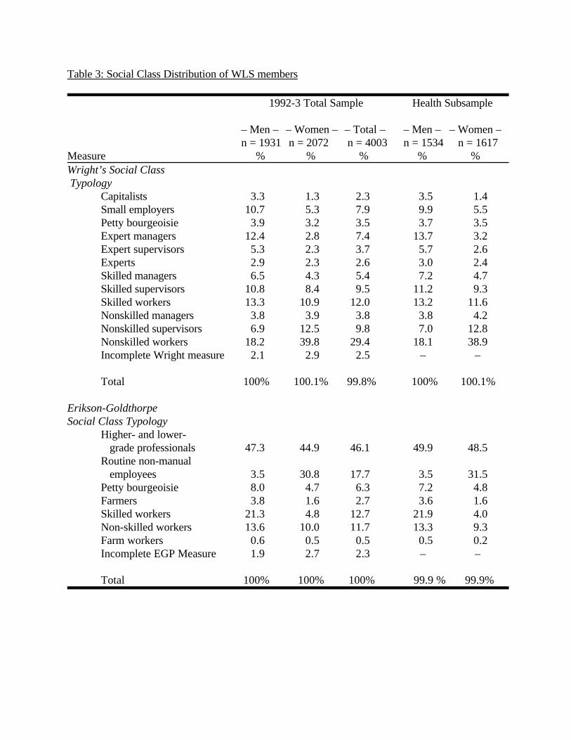
Table 3: Social Class Distribution of WLS members
1992-3 Total Sample Health Subsample
– Men – – Women – – Total – – Men – – Women – n = 1931 n = 2072 n = 4003 n = 1534 n = 1617Measure % % % % %Wright’s Social Class Typology
Capitalists 3.3 1.3 2.3 3.5 1.4Small employers 10.7 5.3 7.9 9.9 5.5Petty bourgeoisie 3.9 3.2 3.5 3.7 3.5Expert managers 12.4 2.8 7.4 13.7 3.2Expert supervisors 5.3 2.3 3.7 5.7 2.6Experts 2.9 2.3 2.6 3.0 2.4Skilled managers 6.5 4.3 5.4 7.2 4.7Skilled supervisors 10.8 8.4 9.5 11.2 9.3Skilled workers 13.3 10.9 12.0 13.2 11.6Nonskilled managers 3.8 3.9 3.8 3.8 4.2Nonskilled supervisors 6.9 12.5 9.8 7.0 12.8Nonskilled workers 18.2 39.8 29.4 18.1 38.9Incomplete Wright measure 2.1 2.9 2.5 – –
Total 100% 100.1% 99.8% 100% 100.1%
Erikson-GoldthorpeSocial Class Typology
Higher- and lower- grade professionals 47.3 44.9 46.1 49.9 48.5Routine non-manual employees 3.5 30.8 17.7 3.5 31.5Petty bourgeoisie 8.0 4.7 6.3 7.2 4.8Farmers 3.8 1.6 2.7 3.6 1.6Skilled workers 21.3 4.8 12.7 21.9 4.0Non-skilled workers 13.6 10.0 11.7 13.3 9.3Farm workers 0.6 0.5 0.5 0.5 0.2Incomplete EGP Measure 1.9 2.7 2.3 – –
Total 100% 100% 100% 99.9 % 99.9%

Table 4: Regressions of Self-Reported Health on Selected Measures of Occupational Standing
– Men – – Women – Variable n = 3137 n = 3344
Siegel Occupational Prestige 0.20 (.04) 0.13 (.04)Intercept 1.13 (.19) 1.53 (.18)
P2 24.24 (1df) 9.68 (1df)BIC 16.19 1.57
Duncan Occupational SEI 0.11 (.02) 0.07 (.03)Intercept 1.47 (.12) 1.74 (.13)
P2 24.39 (1df) 7.46 (1df)BIC 16.34 -0.65
Occupational Education(transformed) 0.21 (.04) 0.14 (.04)Intercept 2.20 (.07) 2.18 (.06)
P2 36.89 (1df) 12.29 (1df)BIC 28.84 4.18
Occupational Income(transformed) 0.23 (.05) 0.08(.04)Intercept 2.20 (.07) 2.26(.11)
P2 24.43 (1df) 3.85 (1df)BIC 16.38 -4.26

Table 4: Regressions of Self-Reported Health on Selected Measures of Occupational Standing(continued)
Men WomenVariable n = 3137 n = 3344Group II Census Classification
Professional, technical and kindred, self-employed and without pay 1.12 (0.40) -0.48 (0.68)Professional, technical and kindred, salaried 0.99 (0.22) 0.27 (0.63)Managers, officials and proprietors, salaried 0.79 (0.22) -0.01 (0.63)Managers, officials and proprietors, self-employed and without pay 0.86 (0.30) -0.05 (0.71)Sales workers, not retail trade 0.83 (0.29) -0.02 (0.69)Sales workers, retail trade 0.34 (0.44) 0.24 (0.69)Clerical and kindred workers 0.52 (0.27) 0.04 (0.62)Craftsmen, foremen and kindred workers, manufacturing reference referenceCrafts, construction 0.44 (0.31) -Crafts, all other 0.70 (0.29) 0.77 (0.95)Operatives, manufacturing 0.24 (0.24) -0.69 (0.65)Operatives, all other 0.09 (0.29) 0.24 (0.77)Service and private household 0.57 (0.30) -0.48 (0.62)Laborers, manufacturing 0.52 (0.77) -Laborers, all other 0.43 (0.51) -0.08 (0.87)Farmers and farm managers 0.07 (0.31) 0.10 (0.81)Farm laborers and farm foremen 0.52 (1.08) -Intercept 1.43 (0.16) 2.12 (0.61)
P2 38.91 (16df) 29.50 (13df)BIC -89.91 -75.99

Table 5: Regressions of Self-Reported Health on Selected Measures of Social Class
– Men – – Women –Variable n = 1534 n = 1617Wright’s Social Class Typology
Capitalists 0.99 (0.63) -0.52 (0.67)Small employers 0.18 (0.32) -0.18 (0.44)Petty bourgeoisie -0.01 (0.43) -0.72 (0.45)Expert managers 0.37 (0.31) -0.13 (0.54)Expert supervisors 0.62 (0.44) -0.12 (0.59)Experts 0.84 (0.63) -0.66 (0.52)Skilled managers 0.27 (0.37) -0.48 (0.43)Skilled supervisors 0.04 (0.30) -0.01 (0.39)Skilled workers reference referenceNonskilled managers 1.10 (0.63) -0.03 (0.50)Nonskilled supervisors -0.09 (0.34) -0.78 (0.32)Nonskilled workers -0.01 (0.27) -0.31 (0.29)Intercept 1.83 (0.20) 2.37 (0.26)
P2 12.75 (11df) 11.23 (11df)BIC -67.94 -70.04
Erikson-GoldthorpeSocial Class Typology
Higher- and lower- grade professionals 0.65 (0.20) -0.06 (0.42)Routine non-manual employees 0.38 (0.46) -0.06 (0.42)Petty bourgeoisie 0.51 (0.35) 0.20 (0.56)Farmers -0.31 (0.37) -0.08 (0.73)Skilled workers reference referenceNon-skilled workers -0.05 (0.24) -0.35 (0.46)Farm workers 0.25 (1.08) -1.42 (1.29)Intercept 1.70 (0.15) 2.11 (0.40)
P2 18.34 (6df) 2.96 (6df)BIC -25.67 -41.37
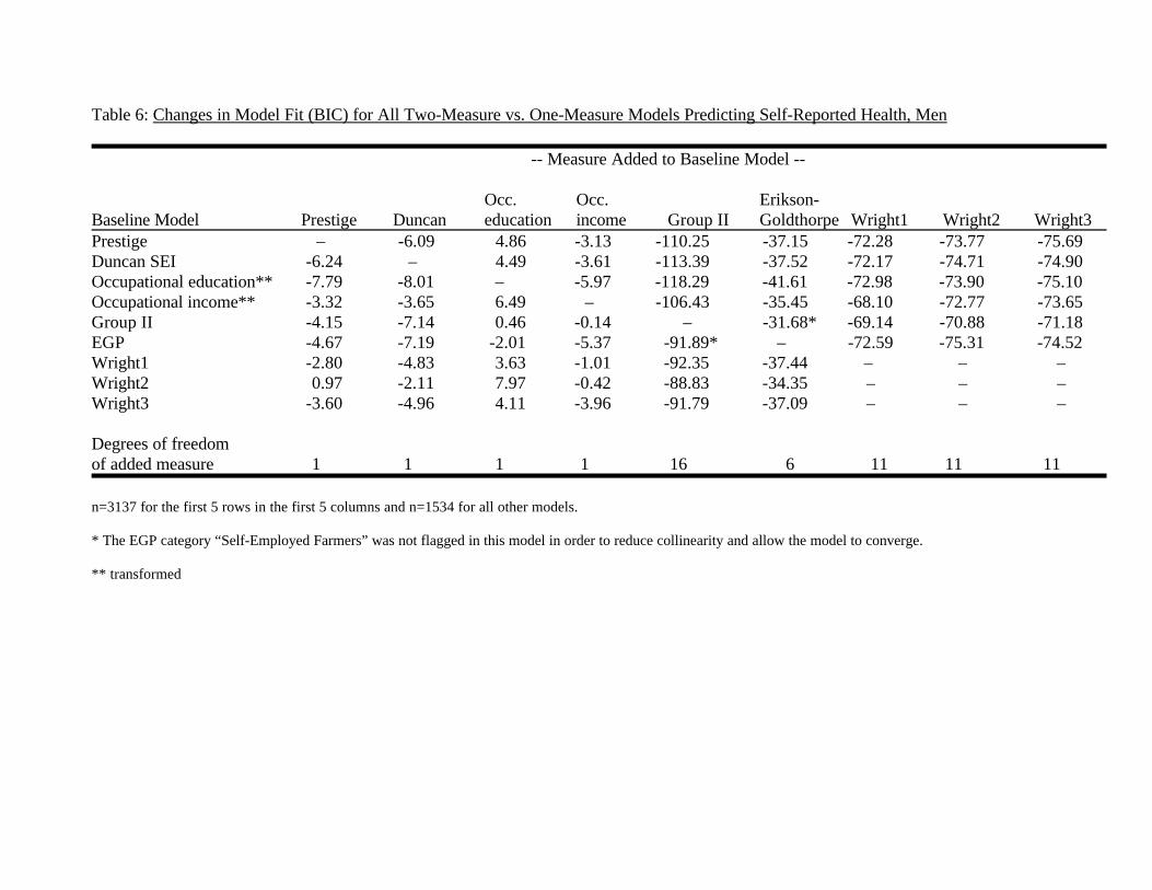
Table 6: Changes in Model Fit (BIC) for All Two-Measure vs. One-Measure Models Predicting Self-Reported Health, Men
-- Measure Added to Baseline Model --
Occ. Occ. Erikson- Baseline Model Prestige Duncan education income Group II Goldthorpe Wright1 Wright2 Wright3Prestige – -6.09 4.86 -3.13 -110.25 -37.15 -72.28 -73.77 -75.69Duncan SEI -6.24 – 4.49 -3.61 -113.39 -37.52 -72.17 -74.71 -74.90Occupational education** -7.79 -8.01 – -5.97 -118.29 -41.61 -72.98 -73.90 -75.10Occupational income** -3.32 -3.65 6.49 – -106.43 -35.45 -68.10 -72.77 -73.65Group II -4.15 -7.14 0.46 -0.14 – -31.68* -69.14 -70.88 -71.18EGP -4.67 -7.19 -2.01 -5.37 -91.89* – -72.59 -75.31 -74.52Wright1 -2.80 -4.83 3.63 -1.01 -92.35 -37.44 – – –Wright2 0.97 -2.11 7.97 -0.42 -88.83 -34.35 – – –Wright3 -3.60 -4.96 4.11 -3.96 -91.79 -37.09 – – –
Degrees of freedom of added measure 1 1 1 1 16 6 11 11 11
n=3137 for the first 5 rows in the first 5 columns and n=1534 for all other models.
* The EGP category “Self-Employed Farmers” was not flagged in this model in order to reduce collinearity and allow the model to converge.
** transformed

Table 7: Changes in Model Fit (BIC) for All Two-Measure vs. One-Measure Models Predicting Self-Reported Health, Women
-- Measure Added to Baseline Model --
Occ. Occ. Erikson-Baseline Model Prestige Duncan education income Group II Goldthorpe Wright1 Wright2 Wright3Prestige – -8.03 -4.90 -7.95 -85.48 -41.46 -72.24 -71.39 -72.44Duncan SEI -8.03 – -3.20 -7.76 -82.65 -41.53 -71.69 -70.68 -69.49Occupational education** -7.51 -8.03 – -8.05 -86.63 -39.49 -72.08 -72.21 -71.94Occupational income** -2.12 -4.15 0.39 – -79.67 -41.26 -72.11 -71.21 -72.29Group II -7.92 -7.31 -6.46 -7.94 – -32.69* -70.57 -70.43 -72.09EGP -5.26 -5.14 -0.40 -5.05 -69.77* – -69.80 -69.08 -70.40Wright1 -6.60 -5.85 -3.54 -6.45 -78.20 -40.35 – – –Wright2 -6.53 -5.63 -4.46 -6.34 -78.85 -40.42 – – –Wright3 -6.35 -5.61 -2.96 -6.19 -79.28 -40.95 – – –
Degrees of freedom ofadded measure 1 1 1 1 13 6 11 11 11
n=3677 for the first 5 rows in the first 5 columns and n=1681 for all other models.
* The EGP category “Self-Employed Farmers” was not flagged in this model to reduce collinearity and allow the model to converge.
** transformed
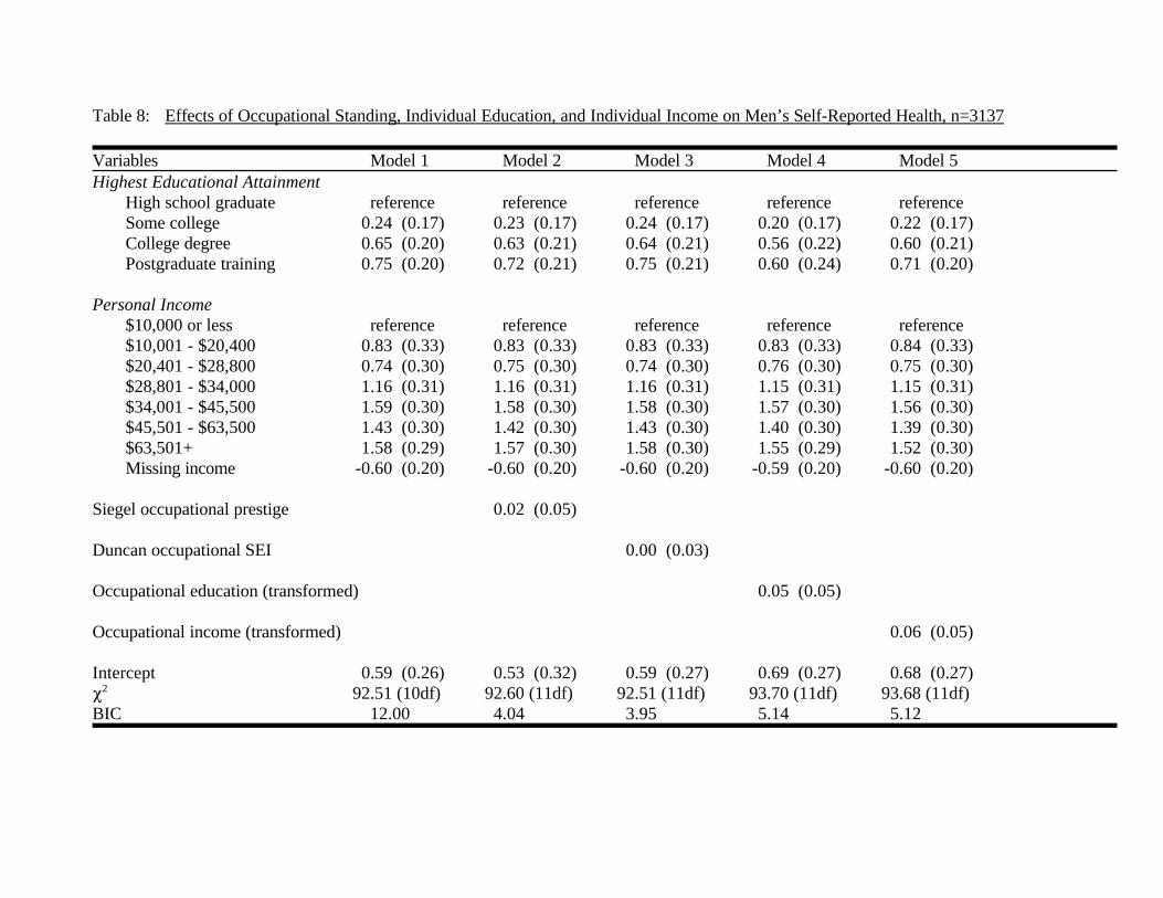
Table 8: Effects of Occupational Standing, Individual Education, and Individual Income on Men’s Self-Reported Health, n=3137
Variables Model 1 Model 2 Model 3 Model 4 Model 5Highest Educational Attainment
High school graduate reference reference reference reference referenceSome college 0.24 (0.17) 0.23 (0.17) 0.24 (0.17) 0.20 (0.17) 0.22 (0.17)College degree 0.65 (0.20) 0.63 (0.21) 0.64 (0.21) 0.56 (0.22) 0.60 (0.21)Postgraduate training 0.75 (0.20) 0.72 (0.21) 0.75 (0.21) 0.60 (0.24) 0.71 (0.20)
Personal Income$10,000 or less reference reference reference reference reference$10,001 - $20,400 0.83 (0.33) 0.83 (0.33) 0.83 (0.33) 0.83 (0.33) 0.84 (0.33)$20,401 - $28,800 0.74 (0.30) 0.75 (0.30) 0.74 (0.30) 0.76 (0.30) 0.75 (0.30)$28,801 - $34,000 1.16 (0.31) 1.16 (0.31) 1.16 (0.31) 1.15 (0.31) 1.15 (0.31)$34,001 - $45,500 1.59 (0.30) 1.58 (0.30) 1.58 (0.30) 1.57 (0.30) 1.56 (0.30)$45,501 - $63,500 1.43 (0.30) 1.42 (0.30) 1.43 (0.30) 1.40 (0.30) 1.39 (0.30)$63,501+ 1.58 (0.29) 1.57 (0.30) 1.58 (0.30) 1.55 (0.29) 1.52 (0.30)
Missing income -0.60 (0.20) -0.60 (0.20) -0.60 (0.20) -0.59 (0.20) -0.60 (0.20) Siegel occupational prestige 0.02 (0.05)
Duncan occupational SEI 0.00 (0.03)
Occupational education (transformed) 0.05 (0.05)
Occupational income (transformed) 0.06 (0.05)
Intercept 0.59 (0.26) 0.53 (0.32) 0.59 (0.27) 0.69 (0.27) 0.68 (0.27)P2 92.51 (10df) 92.60 (11df) 92.51 (11df) 93.70 (11df) 93.68 (11df)BIC 12.00 4.04 3.95 5.14 5.12
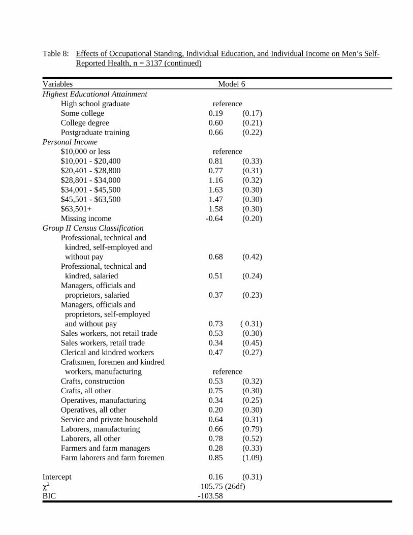
Table 8: Effects of Occupational Standing, Individual Education, and Individual Income on Men’s Self-Reported Health, n = 3137 (continued)
Variables Model 6Highest Educational Attainment
High school graduate referenceSome college 0.19 (0.17)College degree 0.60 (0.21) Postgraduate training 0.66 (0.22)
Personal Income$10,000 or less reference$10,001 - $20,400 0.81 (0.33)$20,401 - $28,800 0.77 (0.31)$28,801 - $34,000 1.16 (0.32)$34,001 - $45,500 1.63 (0.30)$45,501 - $63,500 1.47 (0.30)$63,501+ 1.58 (0.30)
Missing income -0.64 (0.20) Group II Census Classification
Professional, technical and kindred, self-employed and without pay 0.68 (0.42)Professional, technical and kindred, salaried 0.51 (0.24)Managers, officials and proprietors, salaried 0.37 (0.23)Managers, officials and proprietors, self-employed and without pay 0.73 ( 0.31)Sales workers, not retail trade 0.53 (0.30)Sales workers, retail trade 0.34 (0.45)Clerical and kindred workers 0.47 (0.27)Craftsmen, foremen and kindred workers, manufacturing referenceCrafts, construction 0.53 (0.32)Crafts, all other 0.75 (0.30)Operatives, manufacturing 0.34 (0.25)Operatives, all other 0.20 (0.30)Service and private household 0.64 (0.31)
Laborers, manufacturing 0.66 (0.79)Laborers, all other 0.78 (0.52)Farmers and farm managers 0.28 (0.33)Farm laborers and farm foremen 0.85 (1.09)
Intercept 0.16 (0.31) P2 105.75 (26df)BIC -103.58
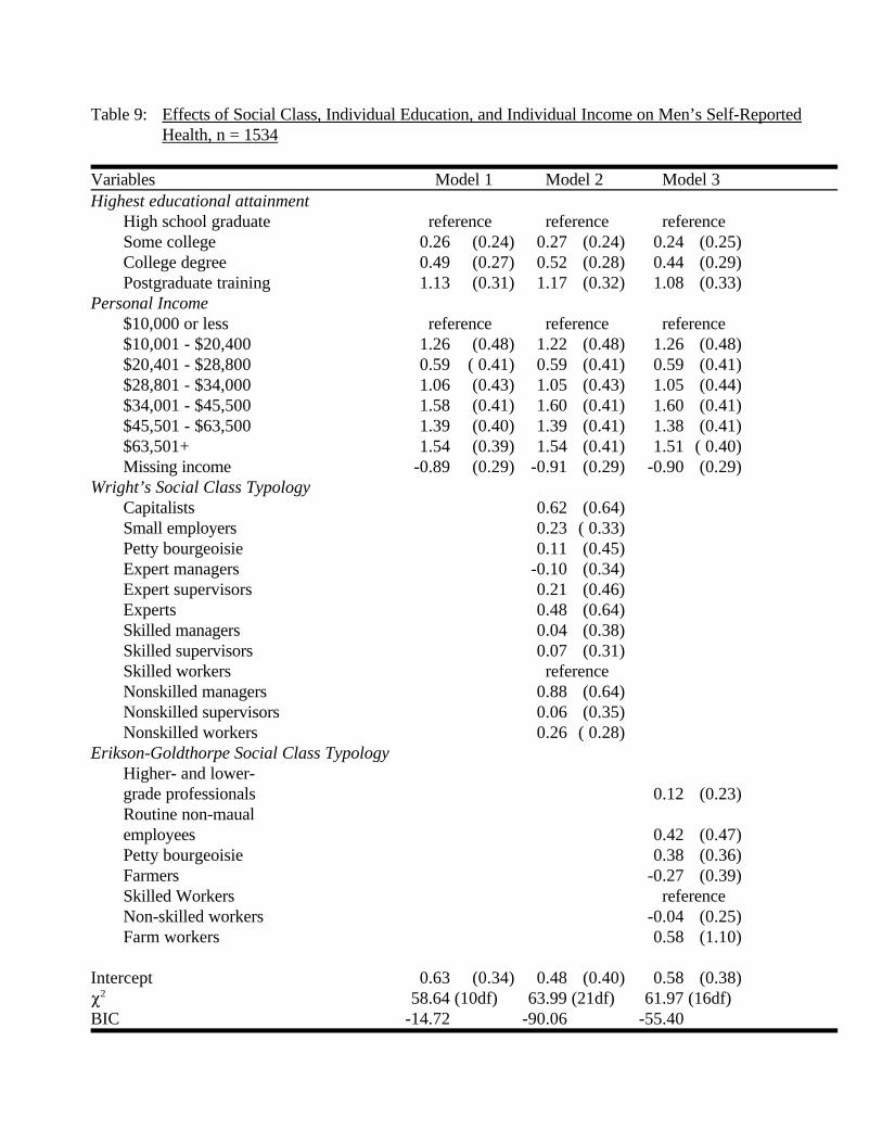
Table 9: Effects of Social Class, Individual Education, and Individual Income on Men’s Self-ReportedHealth, n = 1534
Variables Model 1 Model 2 Model 3Highest educational attainment
High school graduate reference reference referenceSome college 0.26 (0.24) 0.27 (0.24) 0.24 (0.25)College degree 0.49 (0.27) 0.52 (0.28) 0.44 (0.29)Postgraduate training 1.13 (0.31) 1.17 (0.32) 1.08 (0.33)
Personal Income$10,000 or less reference reference reference$10,001 - $20,400 1.26 (0.48) 1.22 (0.48) 1.26 (0.48)$20,401 - $28,800 0.59 ( 0.41) 0.59 (0.41) 0.59 (0.41)$28,801 - $34,000 1.06 (0.43) 1.05 (0.43) 1.05 (0.44)$34,001 - $45,500 1.58 (0.41) 1.60 (0.41) 1.60 (0.41)$45,501 - $63,500 1.39 (0.40) 1.39 (0.41) 1.38 (0.41)$63,501+ 1.54 (0.39) 1.54 (0.41) 1.51 ( 0.40)Missing income -0.89 (0.29) -0.91 (0.29) -0.90 (0.29)
Wright’s Social Class Typology Capitalists 0.62 (0.64) Small employers 0.23 ( 0.33) Petty bourgeoisie 0.11 (0.45) Expert managers -0.10 (0.34) Expert supervisors 0.21 (0.46) Experts 0.48 (0.64) Skilled managers 0.04 (0.38) Skilled supervisors 0.07 (0.31)
Skilled workers reference Nonskilled managers 0.88 (0.64) Nonskilled supervisors 0.06 (0.35) Nonskilled workers 0.26 ( 0.28)Erikson-Goldthorpe Social Class Typology
Higher- and lower-grade professionals 0.12 (0.23)Routine non-maualemployees 0.42 (0.47)Petty bourgeoisie 0.38 (0.36)Farmers -0.27 (0.39)Skilled Workers referenceNon-skilled workers -0.04 (0.25)Farm workers 0.58 (1.10)
Intercept 0.63 (0.34) 0.48 (0.40) 0.58 (0.38) P2 58.64 (10df) 63.99 (21df) 61.97 (16df)BIC -14.72 -90.06 -55.40

Table 10: Effects of Occupational Standing, Individual Education, and Individual Income on Women’s Self-Reported Health, n=3344
Variables Model 1 Model 2 Model 3 Model 4 Model 5Highest Educational Attainment
High school graduate reference reference reference reference referenceSome college 0.24 (0.17) 0.22 (0.18) 0.23 (0.18) 0.21 (0.18) 0.24 (0.18)
College degree 0.56 (0.20) 0.52 (0.21) 0.53 (0.21) 0.49 (0.22) 0.56 (0.21)Postgraduate training 0.39 (0.27) 0.34 (0.27) 0.36 (0.27) 0.31 (0.29) 0.39 (0.27) Personal Income
$0 reference reference reference reference reference$1-,4,400 0.22 (0.33) 0.23 (0.33) 0.23 (0.33) 0.22 (0.33) 0.22 (0.33)
$4,401 - $9,600 0.28 (0.31) 0.29 (0.31) 0.28 (0.31) 0.28 (0.31) 0.28 (0.31)$9,601 - $12,600 0.11 (0.31) 0.11 (0.31) 0.11 (0.31) 0.11 (0.31) 0.11 (0.31)$12,601 - $20,120 0.24 (0.28) 0.23 (0.28) 0.23 (0.28) 0.23 (0.28) 0.24 (0.28)
$20,121 - $30,300 0.40 (0.29) 0.37 (0.29) 0.38 (0.29) 0.38 (0.29) 0.40 (0.29) $30,301+ 0.71 (0.28) 0.68 (0.29) 0.69 (0.29) 0.68 (0.29) 0.71 (0.29)
Missing income 0.12 (0.18) 0.12 (0.18) 0.12 (0.18) 0.12 (0.18) 0.12 (0.18) Siegel occupational prestige 0.04 (0.05)
Duncan occupational SEI 0.02 (0.03)
Occupational education (transformed) 0.04 (0.05)
Occupational income (transformed) 0.00 (0.05)
Intercept 1.60 (0.25) 1.45 (0.30) 1.54 (0.27) 1.66 (0.26) 1.61 (0.27)P2 28.72 (10df) 29.45 (11df) 29.08 (11df) 29.24 (11df) 28.72 (11df)BIC -52.43 -59.81 -60.18 -60.02 -60.54
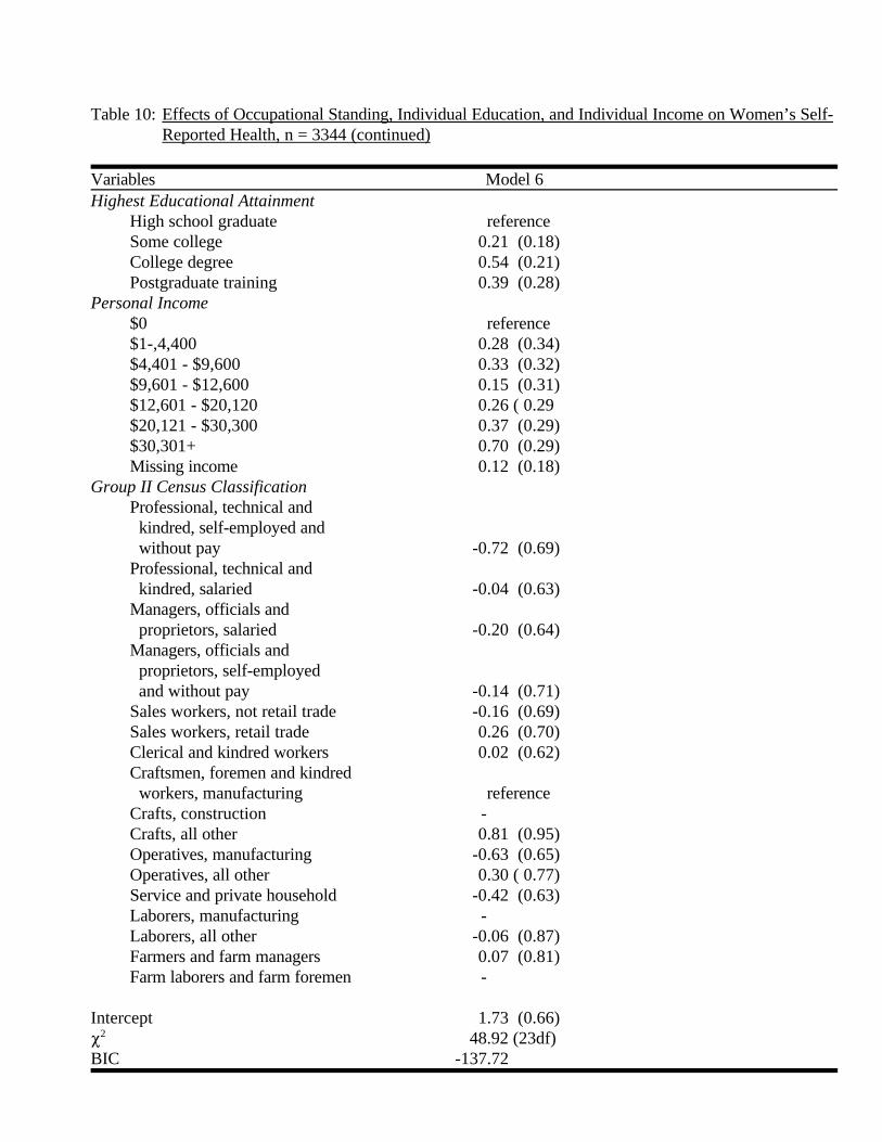
Table 10: Effects of Occupational Standing, Individual Education, and Individual Income on Women’s Self-Reported Health, n = 3344 (continued)
Variables Model 6Highest Educational Attainment
High school graduate referenceSome college 0.21 (0.18)College degree 0.54 (0.21)Postgraduate training 0.39 (0.28)
Personal Income$0 reference$1-,4,400 0.28 (0.34)$4,401 - $9,600 0.33 (0.32)$9,601 - $12,600 0.15 (0.31)$12,601 - $20,120 0.26 ( 0.29$20,121 - $30,300 0.37 (0.29)$30,301+ 0.70 (0.29)
Missing income 0.12 (0.18) Group II Census Classification
Professional, technical and kindred, self-employed and without pay -0.72 (0.69)Professional, technical and kindred, salaried -0.04 (0.63)Managers, officials and proprietors, salaried -0.20 (0.64)Managers, officials and proprietors, self-employed and without pay -0.14 (0.71)Sales workers, not retail trade -0.16 (0.69)Sales workers, retail trade 0.26 (0.70)Clerical and kindred workers 0.02 (0.62)Craftsmen, foremen and kindred workers, manufacturing referenceCrafts, construction -Crafts, all other 0.81 (0.95)Operatives, manufacturing -0.63 (0.65)Operatives, all other 0.30 ( 0.77)Service and private household -0.42 (0.63)Laborers, manufacturing -Laborers, all other -0.06 (0.87)Farmers and farm managers 0.07 (0.81) Farm laborers and farm foremen -
Intercept 1.73 (0.66) P2 48.92 (23df)BIC -137.72
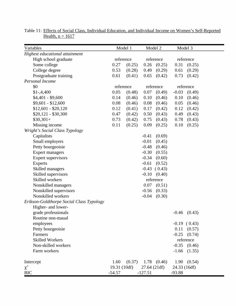
Table 11: Effects of Social Class, Individual Education, and Individual Income on Women’s Self-ReportedHealth, n = 1617
Variables Model 1 Model 2 Model 3Highest educational attainment
High school graduate reference reference referenceSome college 0.27 (0.25) 0.26 (0.25) 0.31 (0.25)College degree 0.53 (0.28) 0.49 (0.29) 0.61 (0.29)Postgraduate training 0.61 (0.41) 0.65 (0.42) 0.73 (0.42)
Personal Income $0 reference reference reference$1-,4,400 0.05 (0.48) 0.07 (0.49) -0.03 (0.49)$4,401 - $9,600 0.14 (0.46) 0.10 (0.46) 0.10 (0.46)$9,601 - $12,600 0.08 (0.46) 0.08 (0.46) 0.05 (0.46)$12,601 - $20,120 0.12 (0.41) 0.17 (0.42) 0.12 (0.42)$20,121 - $30,300 0.47 (0.42) 0.50 (0.43) 0.49 (0.43)$30,301+ 0.73 (0.42) 0.75 (0.43) 0.78 (0.43)
Missing income 0.11 (0.25) 0.09 (0.25) 0.10 (0.25) Wright’s Social Class Typology Capitalists -0.41 (0.69) Small employers -0.01 (0.45) Petty bourgeoisie -0.48 (0.46) Expert managers -0.30 (0.55) Expert supervisors -0.34 (0.60) Experts -0.61 (0.52) Skilled managers -0.43 ( 0.43) Skilled supervisors -0.10 (0.40)
Skilled workers reference Nonskilled managers 0.07 (0.51) Nonskilled supervisors -0.56 (0.33) Nonskilled workers -0.04 (0.30)Erikson-Goldthorpe Social Class Typology
Higher- and lower-grade professionals -0.46 (0.43)Routine non-maualemployees -0.19 ( 0.43)Petty bourgeoisie 0.11 (0.57)Farmers -0.25 (0.74)Skilled Workers referenceNon-skilled workers -0.35 (0.46)Farm workers -1.66 (1.35)
Intercept 1.60 (0.37) 1.78 (0.46) 1.90 (0.54) P2 19.31 (10df) 27.64 (21df) 24.33 (16df)BIC -54.57 -127.51 -93.88

Table 12: Effects of Occupational Standing and Individual Education on Men’s Self-Reported Health, n = 3137
Variables Model 1 Model 2 Model 3 Model 4 Model 5
Highest Educational AttainmentHigh school graduateSome college 0.33 (0.17) 0.28 (0.17) 0.26 (0.17) 0.23 (0.17) 0.26 (0.17)College degree 0.85 (0.20) 0.74 (0.21) 0.73 (0.21) 0.65 (0.21) 0.72 (0.20)Postgraduate training 0.93 (0.19) 0.77 (0.21) 0.79 (0.21) 0.61 (0.23) 0.79 (0.19)
Siegel occupational prestige 0.08 (0.05)
Duncan occupational SEI 0.05 (0.03)
Occupational education (transformed) 0.11 (0.05)
Occupational income (transformed) 0.14 (0.05)
Intercept 1.75 (0.07) 1.42 (0.20) 1.56 (0.12) 1.93 (0.10) 1.90 (0.09) P2 44.12 (3df) 47.08 (4df) 47.34 (4df) 49.47 (4df) 51.26 (4df)BIC 19.97 14.88 15.14 17.27 19.06
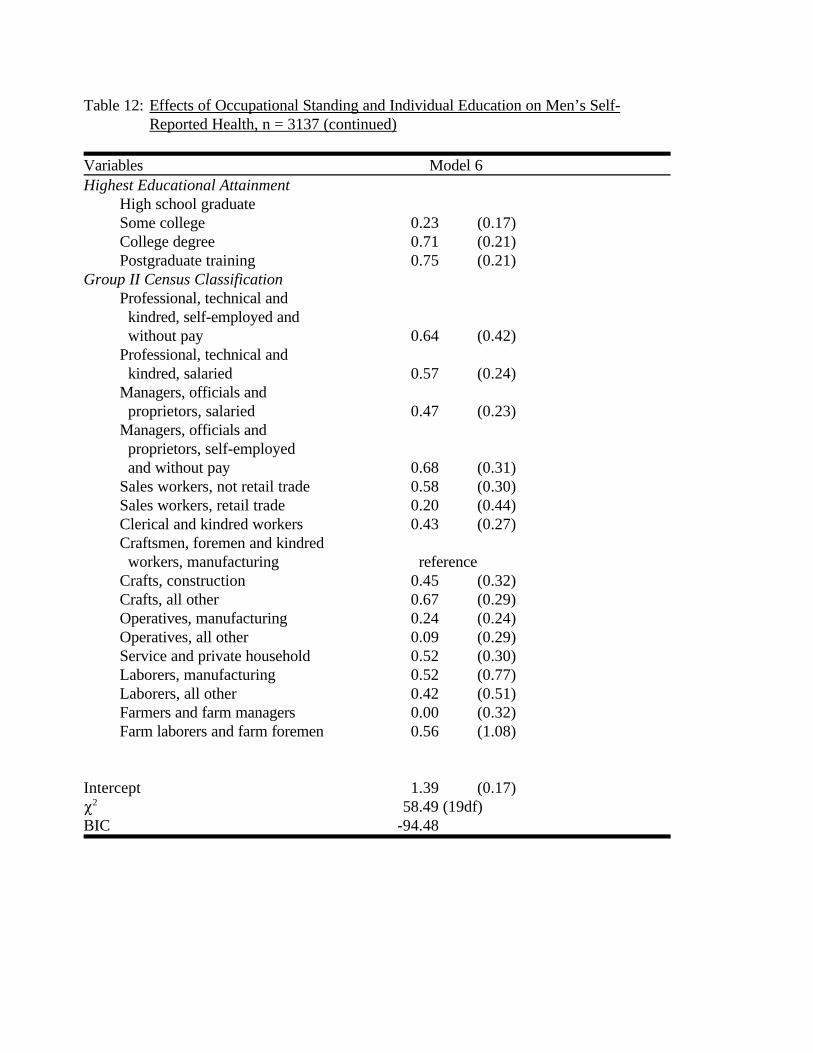
Table 12: Effects of Occupational Standing and Individual Education on Men’s Self-Reported Health, n = 3137 (continued)
Variables Model 6Highest Educational Attainment
High school graduate Some college 0.23 (0.17)College degree 0.71 (0.21) Postgraduate training 0.75 (0.21)
Group II Census ClassificationProfessional, technical and kindred, self-employed and without pay 0.64 (0.42)Professional, technical and kindred, salaried 0.57 (0.24)Managers, officials and proprietors, salaried 0.47 (0.23)Managers, officials and proprietors, self-employed and without pay 0.68 (0.31)Sales workers, not retail trade 0.58 (0.30)Sales workers, retail trade 0.20 (0.44) Clerical and kindred workers 0.43 (0.27)Craftsmen, foremen and kindred workers, manufacturing referenceCrafts, construction 0.45 (0.32)Crafts, all other 0.67 (0.29)Operatives, manufacturing 0.24 (0.24)Operatives, all other 0.09 (0.29) Service and private household 0.52 (0.30)Laborers, manufacturing 0.52 (0.77)Laborers, all other 0.42 (0.51)Farmers and farm managers 0.00 (0.32)Farm laborers and farm foremen 0.56 (1.08)
Intercept 1.39 (0.17) P2 58.49 (19df)BIC -94.48

Table 13: Effects of Social Class and Individual Education on Men’s Self-Reported Health, n = 1534
Variables Model 1 Model 2 Model 3Highest educational attainment
High school graduateSome college 0.31 (0.23) 0.29 (0.24) 0.24 (0.24)College degree 0.71 (0.26) 0.68 (0.27) 0.56 (0.28)Postgraduate training 1.27 (0.30) 1.23 (0.31) 1.12 (0.33)
Wright’s Social Class Typology Capitalists 0.84 (0.63) Small employers 0.21 (0.33) Petty bourgeoisie -0.09 (0.44) Expert managers 0.07 (0.32) Expert supervisors 0.37 (0.45) Experts 0.58 (0.64) Skilled managers 0.18 (0.37) Skilled supervisors 0.09 (0.31)
Skilled workers reference Nonskilled managers 1.01 (0.63) Nonskilled supervisors 0.09 (0.34) Nonskilled workers 0.16 (0.27) Erikson-Goldthorpe Social Class Typology
Higher- and lower-grade professionals 0.24 (0.22)Routine non-maualemployees 0.29 (0.46)Petty bourgeoisie 0.39 (0.35)Farmers -0.41 (0.37)Skilled Workers referenceNon-skilled workers -0.05 (0.24)Farm workers 0.24 (1.08)
Intercept 1.72 (0.10) 1.56 (0.21) 1.65 (0.15) P2 27.95 (3df) 34.32 (14df) 32.82 (9df)BIC 5.94 -68.38 -33.20
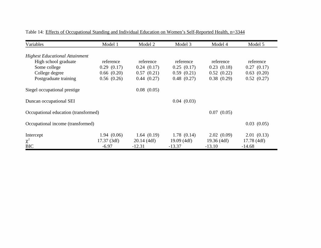
Table 14: Effects of Occupational Standing and Individual Education on Women’s Self-Reported Health, n=3344
Variables Model 1 Model 2 Model 3 Model 4 Model 5
Highest Educational AttainmentHigh school graduate reference reference reference reference referenceSome college 0.29 (0.17) 0.24 (0.17) 0.25 (0.17) 0.23 (0.18) 0.27 (0.17)College degree 0.66 (0.20) 0.57 (0.21) 0.59 (0.21) 0.52 (0.22) 0.63 (0.20)Postgraduate training 0.56 (0.26) 0.44 (0.27) 0.48 (0.27) 0.38 (0.29) 0.52 (0.27)
Siegel occupational prestige 0.08 (0.05)
Duncan occupational SEI 0.04 (0.03)
Occupational education (transformed) 0.07 (0.05)
Occupational income (transformed) 0.03 (0.05)
Intercept 1.94 (0.06) 1.64 (0.19) 1.78 (0.14) 2.02 (0.09) 2.01 (0.13)P2 17.37 (3df) 20.14 (4df) 19.09 (4df) 19.36 (4df) 17.78 (4df)BIC -6.97 -12.31 -13.37 -13.10 -14.68

Table 14: Effects of Occupational Standing and Individual Education on Women’s Self-Reported Health, n = 3344 (continued)
Variables Model 6Highest Educational Attainment
High school graduateSome college 0.23 (0.18)College degree 0.59 (0.21)Postgraduate training 0.50 (0.28)
Group II Census ClassificationProfessional, technical and kindred, self-employed and without pay -0.71 (0.69)Professional, technical and kindred, salaried 0.04 (0.63)Managers, officials and proprietors, salaried -0.11 (0.64)Managers, officials and proprietors, self-employed and without pay -0.12 (0.71)Sales workers, not retail trade -0.12 (0.69)Sales workers, retail trade 0.20 (0.70) Clerical and kindred workers 0.03 (0.62) Craftsmen, foremen and kindred workers, manufacturing referenceCrafts, construction Crafts, all other 0.80 (0.95) Operatives, manufacturing -0.66 (0.65)Operatives, all other 0.26 (0.77) Service and private household -0.47 (0.63)Laborers, manufacturing Laborers, all other -0.09 (0.87)Farmers and farm managers 0.05 ( 0.81) Farm laborers and farm foremen -
Intercept 2.07 (0.61) P2 39.85 (16df)BIC -89.99

Table 15: Effects of Social Class and Individual Education on Women’s Self-Reported Health,n = 1617
Variables Model 1 Model 2 Model 3Highest educational attainment
High school graduate reference reference reference
Some college 0.32 (0.25) 0.31 (0.25) 0.34 (0.25)College degree 0.63 (0.28) 0.58 (0.29) 0.68 (0.28)Postgraduate training 0.82 (0.40) 0.79 (0.42) 0.90 (0.41)
Wright’s Social Class Typology Capitalists -0.30 (0.68) Small employers -0.04 (0.44) Petty bourgeoisie -0.58 (0.45) Expert managers -0.17 (0.54) Expert supervisors -0.17 (0.59) Experts -0.64 (0.52) Skilled managers -0.40 (0.43) Skilled supervisors 0.00 (0.39)
Skilled workers reference Nonskilled managers 0.16 (0.51) Nonskilled supervisors -0.57 (0.33) Nonskilled workers -0.10 (0.30)Erikson-Goldthorpe Social Class Typology
Higher- and lower-grade professionals -0.28 (0.42)Routine non-maualemployees -0.13 (0.42)Petty bourgeoisie 0.16 (0.56)Farmers -0.14 (0.73)Skilled Workers reference
Non-skilled workers -0.35 (0.46)Farm workers -1.66 (1.31)
Intercept 1.88 (0.09) 2.09 (0.28) 2.08 (0.40)
P2 10.83 (3df) 19.41 (14df) 14.25 (9df)BIC -11.33 -84.03 -52.24

Center for Demography and EcologyUniversity of Wisconsin
1180 Observatory Drive Rm. 4412Madison, WI 53706-1393
U.S.A.608/262-2182
FAX 608/262-8400comments to: [email protected] to: [email protected]
Recommended