1
Smart Meter Driven Segmentation: What Your
Consumption Says About YouAdrian Albert, Ram Rajagopal
Abstract—With the rollout of smart metering infrastructureat scale, demand-response (DR) programs may now be tailoredbased on users’ consumption patterns as mined from senseddata. For issuing DR events it is key to understand the inter-temporal consumption dynamics as to appropriately segmentthe user population. We propose to infer occupancy states fromconsumption time series data using a Hidden Markov Modelframework. Occupancy is characterized in this model by i)magnitude, ii) duration, and iii) variability. We show that usersmay be grouped according to their consumption patterns intogroups that exhibit qualitatively different dynamics that maybe exploited for program enrollment purposes. We investigateempirically the information that residential energy consumers’temporal energy demand patterns characterized by these threedimensions may convey about their demographic, household, andappliance stock characteristics. Our analysis shows that temporalpatterns in the user’s consumption data can predict with goodaccuracy certain user characteristics. We use this framework toargue that there is a large degree of individual predictability inuser consumption at a population level.
I. INTRODUCTION
Demand response and energy efficiency programs have
gained wide acceptance as a mechanism to cope with man-
agement of peak load demand in the grid. Such programs
benefit from the heterogeneity in the end user consumption
goals. For example, consumers whose consumption pattern is
more flexible, can be compensated to either curtail or defer
their consumption during peak energy hours. Other programs
target consumers who are inefficient in their consumption due
to long term choices, such as utilizing inefficient appliances or
having poor home thermal insulation. Typical programs offer
rebates in exchange for purchasing more efficient appliances
or pursuing energy efficient interventions at their dwelling.
Due to the heterogeneity in consumer behavior and char-
acteristics, finding the right consumers for the right program
can be costly: it is not feasible to contact every consumer and
obtain demographic, dwelling and behavior information. Fur-
thermore, it is observed that excessive contact with potential
consumers can lead to attrition or loss of enrollment (noted,
e.g., in [11]). Yet, nowadays utilities have at their disposal a
wealth of data about consumers that is not yet extensively used
for improving program performance [33]. Advanced Metering
Infrastructure (AMI) deployments have enabled acquisition
of fine grained energy consumption information which could
Adrian Albert ([email protected]) is with the Electrical Engineeringand Management Science and Engineering Departments, Stanford University,Stanford, CA 94305, USA.
Ram Rajagopal ([email protected]) is with the Civil and EnvironmentalEngineering Department, Stanford University, Stanford, CA 94305, USA.
Manuscript draft May 30, 2013.
reveal various preferences, behaviors and characteristics of in-
dividual consumers. We define smart meter predictive program
segmentation as the problem of uncovering predictive relation-
ships between consumption (as measured by smart meters) and
consumer preferences, characteristics and behaviors. In this
paper we describe this problem in more detail, and propose
a first methodology that captures behaviors at multiple time-
scales and forms to build a predictive segmentation program.
An initial step in uncovering segments of consumers is
building rich, dynamic models of individual consumption; if
such models were available at the individual level, one may
then use them to compare user behavior and relate it with other
available information on socio-demographic characteristics
and user preference. We posit that, when external stimuli
(e.g., weather patterns [32]) are accounted for, individual
temporal consumption depends solely on behavioral choices
(e.g., lifestyle) as reflected in consumption. Moreover, we
hypothesize that these choices stem from socio-demographic
characteristics and attitudes towards energy efficiency. Our
interest here is for a descriptive analysis employing simple
models of consumption. To this end, we i) assess whether
individual users’ (weather-normalized) temporal consumption
patterns is reasonably described using a simple, generative
stochastic model that captures both dynamics and magnitudes
of consumption (a Hidden Markov Model, HMM [29]); ii)
compare and group users according to similarities in their
consumption patterns (using spectral clustering of HMMs [27];
and iii) utilize the inferred characteristics of consumption
to predict exogenous characteristics (demographics, appliance
stock, etc.) To the best of our knowledge, this is the first
paper to propose a dynamic model of consumption for program
segmentation, as well as to predict user attributes and lifestyle
using consumption characteristics.
The rest of the paper is structured as follows. Section II
defines smart meter predictive program segmentation. Section
III reviews the literature on data analytics for smart meters.
Section IV outlines the modelling framework and algorithms
used and how they relate to our application. Section V
describes the data used. Section VI presents a discussion of
consumption characteristics mined from the user population.
Section VII shows that consumption characteristics may be
used to infer user attributes. Section VIII offers a discussion
of how this methodology may be used in practice for targeted
incentive programs. Section IX concludes the paper.
II. PROBLEM STATEMENT
Predictive program segmentation. We observe N time series
{X}n, n = 1, ...N , each representing the energy consumption

2
(in kWh) sampled at regular intervals ∆t (here 30-minute
aggregates of 10-minute data) of an individual household n(here referred to interchangeably as users or individuals). Our
goal is to derive characterizations of individual consumption
across a user base as to identify segments in the population
whose usage patterns are in some way similar. Users in differ-
ent groups have different inter-temporal consumption decision
dynamics, and should benefit from different consumption
curtailment strategies. From a system operator’s perspective,
the demand of users with less predictable temporal consump-
tion profiles is more expensive to service than for those
whose consumption one can predict well [5]. Yet demand-
response programs may also benefit from diverse load patterns:
with proper aggregation and control mechanisms (differential
pricing, incentives for load deferral etc.), one may achieve
load-balancing results building on the relative flexibility in
consumption of more random users. Moreover, it is expected
that people sharing similarities on certain levels (lifestyle,
appliances, house characteristics for the energy context) will
generally exhibit similar characteristics in consumption. This
hypothesis has been hard to validate in the past because of
insufficiently detailed metered data. We propose a data-driven
methodology that allows predicting user attributes using only
consumption characteristics as inferred from the consumption
time series. The steps are outlined below and in Figure 1.
Fig. 1. Schematic of the analysis presented in this paper (see Section II).
Dynamic user consumption model. For each user, we model
energy use as the sum of a deterministic weather sensitivity
component and an occupancy component:
Xt = f(Wt) + Yt, (1)
where Wt are exogeneously-specified weather time series, f(·)is a functional form specified by the modeler (here linear-in-
parameters, see Section V), and Y is an occupancy-related
component. Note that we explicitly adopted the simplification
that weather and occupancy are independent, which is a strong
assumption to make; subsequent extensions on this basic
model will address this issue (see Section IX).
What we here term “occupancy” is in fact a proxy for a
combination of i) number of household members and their
presence in the house, and ii) their activity while at home.
In a real-world situation we do not observe ground-truth
labels of the different activities over time that result in energy
consumption decisions; but can we identify certain patterns
that are associated with more high-level lifestyle and appliance
ownership proxies?
Modeling each consumer separately has several advantages:
i) having a separate model for each user more richly cap-
tures the individual characteristics for personalized targeting
strategies; ii) the computation is easily parallelizable, as no
dependencies across users are taken into account; and iii) new
AMI deployments and data storage and processing capabilities
are making possible to analyze consumption at the individual
level, offering identification properties and rich structure pre-
viously only available from panel-type analyses.
The predominant approach to modelling energy consump-
tion has focused on the first component of (1), primarily
by specifying a linear form of f(·) on weather {Wt}. We
formulate a typical linear regression model in Section V;
however, we argue there that this modelling choice leaves
out important structure in the idiosyncratic component of the
regression. In particular we observe a large degree of serial
correlation and departure from the assumption of normality.
Even when (linear) deterministic weather effects are accounted
for, some users may display a bursty, relatively predictable
consumption behavior, whereas others may appear to consume
rather at random. I.e., the linear model predicts consumption
well for some users, but fails to do so for others.
Our contribution is to explicitly model the idiosyncratic
component Y , which we interpret as encoding occupancy
effects on consumption. We posit that consumption follows
an inter-temporal sequence of decisions that describe occu-
pancy states of a household in addition to the (deterministic)
baseline provided by weather. We wish to propose simple
characterizations of the occupancy states in terms of mag-
nitude, duration, and variability. Thus consumption may be
represented schematically as in Figure 2, with the magnitude
dimensions (µ, σ2) on the horizontal and vertical axis, the
duration dimension represented by the radius of the circles (λ),
and variability represented by the grayscale intensity of the
transition arrow between the two states. A natural modelling
choice for that end is a Hidden (Semi-)Markov Model.
Fig. 2. Consumption characteristics: magnitude µ, duration λ, variability S.
Model-based user classes. For the purpose of intervention
programs, we want to group our N time series into K ≪ Ntypes, so that each group may receive a tailored incentive. In

3
practice it is critical to have a small enough K (to reduce
administrative costs and user confusion), yet to capture the
temporal dynamics structure in the data well. Given the non-
linear fashion in which these patterns interact across users, we
employ unsupervised learning techniques to compute group-
ings starting from the individual models for consumption.
These groups are natural targeting segments for marketing
demand-response programs.
User and consumption characteristics. Having characterized
individual consumption according to weather sensitivity, mag-
nitudes, duration, and variability, we wish to relate such struc-
ture to user attributes. We are interested in prediction power
of model features with respect to lifestyle- and appliance-
related attributes of users. This approach is the inverse of the
current practice at utilities, which perform “psychographic”
segmentation that attempts to infer consumption patterns from
questionnaire data administered to customer sample [25].
III. LITERATURE REVIEW
Energy consumption has been of significant interest for a
number of literatures, in particular economics and engineering.
Econometric studies are typically concerned with user demand
elasticity in the presence of non-linear pricing and deregula-
tion (e.g., [31], [32]). Another topic that has received much
attention has been the effect of weather on residential energy
use. For example, in [15] the authors argue for a non-linear
dependence of energy consumption with temperature, whereas
in [12] the authors propose a specification that uses lagged
temperature values. In [16], the authors use the same dataset
as us in a panel format to estimate econometrically the effects
of real-time feedback on consumption. However until recently
most such studies could only use daily or monthly data.
Because of the unavailability of high-resolution, hourly
or sub-hourly meter data, the literature on energy analyt-
ics energy is still in its infancy. Some recent works use
low-resolution consumption data for more recent statistical
learning algorithms to improve on forecasting performance of
early work. For example, in [21] the authors apply Gaussian
process regression to monthly energy consumption data for
residential buildings and household characteristics obtained
from databases to predict energy usage at a city block level.
With the recent introduction of smart meters at scale, more
(mostly application-oriented) studies have been published that
address high resolution time series modeling or customer
clustering. For example, [33] challenges the assumption in
the load analysis practice of morning and evening peaks by
using a large time series corpus to identify 40 typical load
shapes using K-Means clustering. In [10] the authors use 15-
minute resolution smart meter data from ∼ 200 customers of
an utility company in Germany to perform a K-Means clus-
tering analysis to inform cluster-based pricing schemes. They
propose time-varying prices that are a function of the “num-
ber of peaks” and peak width, which essentially are rough
measures of consumption dynamics. In [30] a features-based
(K-Means) clustering is proposed using quantities such as
the mean, standard deviation, maximum Lyapunov coefficient,
Fourier mode energy for each of the 11 weeks and the ∼ 1000
customers in their data. A similar approach is taken also in
e.g., [9]. More closely related to our analysis methodology, [2]
identifies groups of substations in the Belgian grid based on
daily load patterns at 245 buses using a multivariate version
of spectral clustering. Also, [19] analyze the same dataset
[16] from the perspective of structural building characteristics
effects on season-adjusted consumption statistics. Recently [1]
have proposed a statistically-meaningful customer segmenta-
tion technique that is based on Power Demand Distributions,
i.e., recurring shapes in consumption distribution profiles.
Extensive literature exists on HMMs [29] and on their
many flavors and applications, ranging from DNA structure
analysis to speech recognition to financial market modeling.
Here we use Hidden Semi-Markov Models (HSMMs) [39].
Typical computational issues include estimating the number of
states [4] and dealing with missing data [37]. In the context
of residential load data, HMMs have only seen a limited use
to date, in particular for the disaggregation problem of re-
covering individual appliance signals from the aggregate load
profile [22], [20]. Recently HMMs have been adopted with
enthusiasm also in the targeted interventions and marketing
literatures. For example, in [26] the authors estimate a model
of the dynamics of alumni-university relationship using a panel
of donation data. Over the last decade a growing interest is
noticeable in incorporating external covariates into the HMM
framework, which is most commonly done using generalized
linear (e.g., logit) models for rows of the transition matrix and
linear regression models for the state emission probabilities
[36], [40]. Recently a growing body of literature developed
estimation methodologies for such models defined over an
entire population (in a panel fashion) [40].
Segmenting a collection of time series using Hidden Markov
Models is also a relatively new thread of research. In a
clustering application, direct comparison of the parameter
space of two models is ill defined, as the models may differ
greatly in complexity [17]. Different techniques [34], [23],
[17], [38] have been proposed to learn clustering solutions for
HMM collections which typically involve computing a log-
likelihood matrix L of every time series under each of the
models, and then applying a standard clustering algorithm on
L (or a suitable transformation thereof), such as K-Means
or spectral clustering [27]. Other, fully-parametric approaches
view the K-clustering problem as estimating a mixture of KHMMs on the entire dataset [6]. The analysis presented in this
paper more closely resembles that in [17] and [38], as we use
a combination of parametric and unsupervised learning.
IV. ALGORITHMIC FRAMEWORK
A. Hidden Markov Models
We propose to model the time-dependent occupancy effects
on consumption for an individual user as a trajectory through
occupancy states. Each state is characterized by magnitude
and duration spent in the state as described in Figure 2.
Moreover, the dynamics of transitioning between the states
is modeled as a (discrete) stationary process. As we argue in
Section V, a large degree of serial correlation is observable
empirically in the consumption time-series. This suggests that
4
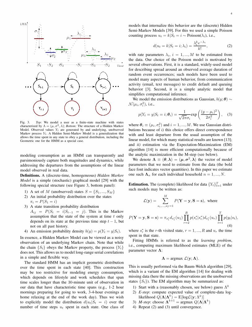
Fig. 3. Top: We model a user as a finite-state machine with statescharacterized by Λ = (µ, σ2, λ); Bottom: The structure of a Hidden MarkovModel. Observed values Yt are generated by and underlying, unobservedMarkov process Yt. A Hidden Semi-Markov Model is a generalization thatallows the time spent in any state to obey a general distribution, including theGeometric one for the HMM as a special case.
modeling consumption as an HMM can transparently and
parsimoniously capture both magnitudes and dynamics, while
addressing the departures from the assumptions of the linear
model observed in real data.
Definitions. A (discrete-time, homogeneous) Hidden Markov
Model is a simple (stochastic) graphical model [29] with the
following special structure (see Figure 3, bottom panel):
1) A set of M (unobserved) states S = {S1, ..., SM}2) An initial probability distribution over the states
πi = P (S1 = i)3) A state transition probability distribution
Aij = P (St = i|St−1 = j). This is the Markov
assumption that the state of the system at time t only
depends on its state at the previous time step t− 1, but
not on all past history.
4) An emission probability density b(y) = p(Yt = y|St).
In essence, a Hidden Markov Model can be viewed as a noisy
observation of an underlying Markov chain. Note that while
the chain {St} obeys the Markov property, the process {Yt}does not. This allows us to model long-range serial correlations
in a simple and flexible way.
The standard HMM has an implicit geometric distribution
over the time spent in each state [40]. This construction
may be too restrictive for modeling energy consumption,
which depends on lifestyle and work schedules that span
time scales longer than the 30-minute unit of observation in
our data that have characteristic time spans (e.g., 1-2 hour
mornings preparing for going to work, 3-4-hour evenings at
home relaxing at the end of the work day). Thus we wish
to explicitly model the distribution d(ut|St = i) over the
number of time steps ut spent in each state. One class of
models that internalize this behavior are the (discrete) Hidden
Semi-Markov Models [39]. For this we used a simple Poisson
counting process ut = k|St = i ∼ Poisson(λi), i.e.,
d(ut = k|St = i;λi) =λki e
−λi
k!, (2)
with rate parameters λi, i = 1, ...,M to be estimated from
the data. Our choice of the Poisson model is motivated by
several observations. First, it is a standard, widely-used model
for describing spread around an observed average duration of
random event occurrences; such models have been used to
model many aspects of human behavior, from communication
activity (email, text messages) to credit default and queuing
behavior [3]. Second, it is a simple analytic model that
simplifies computational inference.
We model the emission distributions as Gaussian, b(y; θ) ∼N (µi, σ
2i ), i.e.,
p(Yt = y|St = i; θi) =1√2πσi
exp
(
(y − µi)2
2σ2i
)
, (3)
where θi ≡ (µi, σ2i ) and i = 1, ...,M . We use Gaussian distri-
butions because of i) this choice offers direct correspondence
with and least departure from the usual assumption of the
linear model, for which many statistical results are known [13];
and ii) estimation via the Expectation-Maximization (EM)
algorithm [14] is more efficient computationally because of
the analytic maximization in the M-step (see below).
We denote Λ ≡ (θ,λ) = (µ,σ2,λ) the vector of model
parameters that we need to estimate from the data (the bold
face font indicates vector quantities). In this paper we estimate
one such Λn for each individual household n = 1, ..., N .
Estimation. The (complete) likelihood for data {Yt}Tt=1 under
such models may be written as:
L(y) =M∑
s1,...,sT=1
P (Y = y,S = s), where
P (Y = y,S = s) = πs∗1ds∗
1(u1)
R∏
r=2
p(s∗r |s∗r)ds∗1 (ur)
T∏
t=1
p(yt|st),
(4)
where s∗r is the r-th visited state, r = 1, ..., R and ur the time
spent in that state.
Fitting HMMs is referred to as the learning problem,
i.e., computing maximum likelihood estimates (MLE) of the
parameter vector Λ:
Λ = argmax L(y;Λ).
This is usually performed via the Baum-Welch algorithm [29],
which is a variant of the EM algorithm [14] for dealing with
missing data (here the missing observations are the unobserved
states {St}). The EM algorithm may be summarized as:
1) Start with a (reasonably chosen, see below) guess Λ0
2) E-step: compute expected value of complete-data log-
likelihood Q(Λ|Λk) = E[logL(y; Λk)]3) M-step: choose Λk+1 = argmax Q(Λ|Λk)4) Repeat (2) and (3) until convergence.

5
Explicitly modeling durations ur above complicates learning,
but a number of efficient estimation methods have been
developed for the task. Here we used the exposure and
implementation in [28].
Note that the solution the EM algorithm converges to is
typically a local maximum of the likelihood function. This
is because L is non-convex in general. Careful initialization
of model parameters or multiple re-estimations starting from
different initialization points may ensure that a good such
local optimum is found that is close to the global optimum.
Following [23], here we first computed a K-means clustering
on M (the number of HMM states) of the observation data y;
for each of those clusters we computed the mean and variance
of the observations contained, which we then used as initial
estimates for state means and variances.
Inference (computing the most likely sequence of states s
that fits a given observation sequence y) is referred to as the
decoding problem in the HMM literature:
argmaxs
P (S|Y).
Efficient inference (the Viterbi algorithm [29]) that is based
on dynamic programming is known for this problem. We use
the implementation provided in the [28] in our calculations.
Choosing model size. The discussion above assumes that
the number M of states is known a priori; this is not the
case when dealing with real data. Many approaches have been
proposed that address this problem in particular contexts [24];
here we employ a strategy outlined in [4]: for a given time
series we fit an HSMM with a maximum allowed number of
states Mmax (here Mmax = 10) to the training set (about half
of the observations); we then sequentially prune out the least
probable state in the stationary distribution of the underlying
Markov Chain, each time computing a measure of model fit
(here the BIC criterion [14]) on a validation set (of similar
size to the training set); we finally choose the optimum model
size M∗ the one with the highest BIC score.
B. HMM clustering
As in [23], [17], we use spectral clustering to segment a
collection of HMMs into classes of similar statistical prop-
erties. This is a graph-theoretic segmentation technique that
relies on solving a minimum cut problem in a weighted graph
[27]. For a K-clustering problem, the algorithm is as follows:
1) compute a N ×N symmetric matrix W , where
Wij = |p({Yt}j ;Λi) + p({Yt}i;Λj)−p({Yt}i;Λi)− p({Yt}j;Λj)|, (5)
for all pairs of sequences {Yt} and HMM fits Λ;
2) compute the normalized Laplacian L of the graph de-
fined by the adjacency matrix exp(−Wij/2σ2) (for σ2
chosen as described in [27])
3) compute the K principal eigenvectors corresponding to
the largest eigenvalues of L and use them to form a new
stacked N ×K matrix P ;
4) apply a standard clustering algorithm (here we used
K-Medoids) on P , and output cluster membership.
Fig. 4. Geographic distribution and climate zones of users in the sample.
V. EXPERIMENTAL SETUP
A. Data description
Question Levels Answers
Individuals.under.5 No/Yes 615/337
Individuals.36.to.54 No/Yes 546/406
Individuals.55.to.65 No/Yes 893/59
Individuals.over.65 No/Yes 927/25
Pets No/Yes 573/379
Employed.full.time outside.home. No/Yes 14/938
Employed.part.time outside.home. No/Yes 835/117
Work.from.home No/Yes 788/164
Unemployed. No/Yes 669/283
Central.Heater Other/Electricity 763/189
Spa.Hot.Tub.or.Pool.Heater Other/Electricity 870/82
Water.Heating.Systems Other/Electricity 814/138
Clothes.Dryer Other/Electricity 366/586
Oven Other/Electricity 435/517
Cooktop.Stovetop Other/Electricity 615/337
Plasma.Televisions No/Yes 670/282
Non.plasma.Televisions No/Yes 180/772
Refrigerators < 2/ >= 2 699/253
Computers < 2/ >= 2 52/900
DVD.players No/Yes 61/891
Gaming.Consoles No/Yes 300/652
Dishwashers No/Yes 53/899
Stand.alone.Freezers No/Yes 821/131
Washing.Machines No/Yes 91/861
Clothes.Dryers No/Yes 94/858
Room.Units.or.Central.AC No/Yes 339/613
Stand.alone.Unit.or Central.Heaters No/Yes 70/882
Spas.Hot.Tubs.or.Pools No/Yes 829/123
TABLE IQUESTIONNAIRE SUMMARY (APPLIANCES AND DEMOGRAPHICS)
The primary dataset used in this paper was collected through
an 8-month (March-October 2010) experiment [16]. The orig-
inal goal of the study was to assess the impact of detailed con-
sumption feedback on energy use. Data is available from about
1100 households of U.S-based Google employees and contains
i) Power demand time series of 10-minute resolution for about
1100 households and ii) Socio-economic data obtained via
an on-line survey in which approximately 950 participants
took part. In addition to this data we collected measurements
on weather parameters (at 5 − 15 minutes resolution) at
the locations (indicated by zipcode) of most users in the
experiment using an online API1. The geographic distribution
1www.weatherunderground.com

6
(and the corresponding weather patterns) experienced by the
users varied substantially across the population (see Figure 4).
Most users however were located in Northern California.
Data was not free of inconsistencies (e.g., reading errors or
incorrect timestamps); some time series contained very few
data points (less than 200), such that they were left out of the
final analysis. In addition, we only retained those households
(N = 952) for which survey responses were available, and for
which reliable fine-grained weather data could be collected.
We snapped both the weather covariates and the consumption
time series to the same time axis using nearest-neighbor
interpolation to fill in small gaps (up to 2 hours) and an EM
algorithm (package Amelia in R with a multivariate normal
target distribution) to imputate gaps for up to a day.
The online survey included information on many socio-
demographic characteristics (we selected 89 covariates of
interest, leaving out information such as political orientation
and gender). A summary of some selected important attributes
is given in Table I. For the purpose of this analysis, we
were only interested in practical dichotomies on participant
characteristics, e.g., whether a given household had a large
number (> 2) of fridges, or had any elderly people or infants.
B. Weather effects
We estimate the (linear) weather effects in (1) as f(W ) by
performing a regression analysis of the form
xnt =
9∑
j=1
βnjWnt +
24∑
j=1
δnj1{ToD(t) = j}+
7∑
j=1
γnj1{DoW(t) = j}+ νn1{Holiday(t)} + ǫnt,
(6)
where n ∈ {1, ...N} refers to the user n as before, t ∈{1, ...T } represents time (on a 30-minute resolution), Wnt are
the weather covariates (temperature, pressure, humidity, and
second-order interactions) for user n, the δ’s, γ’s and the ν’s
are dummy variables for time-of-day (in hours), day-of-week
(Monday to Sunday) and federal holiday, respectively. We
settled for specifying hourly and weekly fixed effects this way
as opposed to defining a more flexible day-of-week to hour-
of-day interaction terms because of the more stringent data re-
quirements for estimating the latter specification (24×7 = 168coefficients as opposed to 24 + 7 = 31 coefficients in the
former case). The ǫnt terms are normally-distributed with zero
mean (an ordinary least-squares regression). We used higher
powers of weather covariates following [15], who argue for an
up to fourth-order polynomial dependence with temperature of
energy use based on a physical model of heat loss. The object
of analysis in the next sections is the regression residuals ǫntwhich, according to Figure 5 accounts for a significant portion
of consumption: around 80% of variance in consumption for
most users, and up to 35% of variance for even the users
best-represented by linear models. Designing programs and
evaluating their performance based on models with such poor
predictive capabilities clearly miss important opportunities.
Fig. 5. Distribution of variance explained (R2 , expressed as fraction) byweather (overall and per-covariate) for all users in the sample.
As Figure 5 suggests, regression performance varies quite
widely across the panel of users in explaining variance in
consumption. Taken individually, weather covariates don’t
exhibit significant performance, with the best of the three
being temperature (up to ∼ 30% variance explained for some
users) and the worst being humidity (green curve). However,
the model (6) explains up to ∼ 65% of the variance in
consumption depending on the user. We retained the regression
coefficients as classification features (Section VII).
C. Beyond the linear model: the case for occupancy effects
Note that important assumptions on the idiosyncratic shock
ǫnt in linear models such as (6) are independence and identical
distribution (i.i.d) according to a normal distribution (with
constant variance) [13], i.e.,
E[ǫntǫnt′ ] = 0 and
ǫnt ∼ N (0, σ2). (7)
These are very restrictive assumptions that do not necessarily
hold in real consumption data, even with flexible specifications
of the deterministic part in (6). For example, consider Figure 6,
where we present some properties of the regression residuals
for one typical user. The residual density (lower-left panel)
is clearly non-Gaussian, with apparent secondary peaks and a
long tail, which suggests a mixture structure. Moreover, the
autocorrelation coefficients for the first 15 lags (lower-right
panel) are significantly greater then 0 (well above the 5%
confidence level indicated by the horizontal dashed line).
We performed a similar analysis on the residuals for all
users in our sample. First, we observe a high degree of het-
eroskedasticity (unequal variance σ2 at different observations).
In fact, of the ∼ 1000 users that we perform our analysis on,
> 94% display noticeable heteroskedasticity (as detected using
a standard Breusch-Pagan test at a 5% level [13]). Second, we
investigated the departure from normality of consumption for
users in the sample, using an Anderson-Darling test of the
null hypothesis H0 that the data was drawn from a normally-
distributed population [13], and find that we are able to reject
H0 at a 5% confidence level for 83% of the users in the
sample. To test for serial correlation we used a Durbin-Watson
test [13] (which tests H0 that the first-order autocorrelation
lag ρ = 0), and find that we are able to reject H0 at a 5%confidence level for all (100%) the users in our sample. All

7
Fig. 6. Structure of the linear model error term for one example user. A timeseries of the residuals is shown in the upper panel. Note the non-Gaussiandistribution density (lower-left panel) and the significant autocorrelationcoefficients (lower-right panel, bars above the dotted blue line) for lags up to16 (8 hours).
these observations are clear indication that there is more to
consumption that is not captured by the simple linear model
that is pervasive in the energy consumption analysis literature.
VI. OCCUPANCY STATES ANALYSIS
A. Characteristics of consumption
The analysis in this section proceeds on the occupancy
component of consumption Y in our model (1). To each user’s
occupancy component Y we fit time-homogeneous HSMMs
with Gaussian emission distributions and Poisson sojourn
times, as outlined in Section VII and following the exposure
in [28]. All estimations were performed in the open-source
statistical language R. Model structure for an example user is
illustrated in Figure 7. The top panel presents the decoded
sequence for about 5 days, with the means (colored dots)
and standard deviations (vertical gray bars) of the inferred
states plotted over the actual consumption (gray). Note that
such a model is able to capture both the bursty events in
consumption (the high-mean, high-variance state 3 depicted
in green) and the relative flat consumption periods (state 5
depicted in magenta). The bottom-left panel is an illustration
of the consumption characteristics of the occupancy states for
the selected users following the schematic in Figure 2, in
which each state is a circle of radius λ in a (µ,σ2)-space. Link
widths are proportional to the transition probabilities between
states and encode variability in consumption. The bottom-right
panel compares the first 40 autocorrelation coefficients of the
residuals ǫit for the sample user with those of the the HSMM
fit. Such a model is (by construction) able to capture the long-
range correlations in consumption to a significant degree at
least for the first ∼ 10 lags (corresponding to 5− 6 hours).
In Figure 8 we show the distribution of variance explained
R2 and model size M for the user population. Such modeling
explains, on average, another ∼ 35% of the variance in the
OLS residual, and as high as 80%. Most common model
complexity is 5 states; note that the truncation at M > 10was done for computational reasons (since the Baum-Welch
has a runtime complexity quadratic in M , O(TM2)). There is
wide variation on performance, which indicates that our simple
modeling steps may not be sufficient for capturing the complex
nature of consumption for certain users. We are currently
developing a user model with superior predictive properties
building upon the observations in this paper.
A general trend we notice in the case of magnitude charac-
teristics (state mean µ and variance σ2) is that the first four
states tend to represent consumption levels below the baseline
offered by the deterministic weather part in (1); models with
5 or more states represent complex dynamics including more
pronounced bursty consumption. We also notice that typical
sojourn times (rates λ of Poisson durations) range from 2-
4 time steps (1-2 hours) to upwards of 50 timesteps (a
whole day). This indicates a large degree of heterogeneity in
occupancy regimes for single users and across a population.
B. Occupancy variability
To quantify empirically the randomness in the HSMM state
sequence describing each individual user’s consumption as es-
timated above, we turn to information-theoretic concepts. The
(Shannon) entropy of a discrete (over M states), stationary,
i.i.d. stochastic process with known p.m.f p is given by
Sshn = −M∑
j=1
p(j)log2p(j). (8)
In our case p(·) is defined over sequences [7]. To approxi-
mately compute the entropy of arbitrary sequences for a finite,
discrete-time process, we use the Lempel-Ziv estimator [35]
SLZ =
(
1
T
∑
i
li
)
−1
lnT, (9)
with T the length of the sequence and li the length of the
shortest substring that starts at position i and which does not
appear at any position between 1 and i − 1. In addition, we
compute two additional benchmarks to characterize variability
of the occupancy states under different models for p(·). If pis the uniform distribution, we have Srnd = log2(M). If pis the limiting distribution π of the underlying Markov chain
(the left-eigenvector of the transition matrix A,π = Aπ), we
have Sshn = −∑M
j=1πj log2πj . In Figure 9 (left panel) we
present the distribution of the three benchmarks Srnd, Sshn,
and SLZ over all users in the sample. Note that SLZ peaks
at ∼ 1.5 (corresponding to an average uncertainty of 21.5 <3 states), whereas Sshn peaks at ∼ 2.4 (corresponding to an
uncertainty ∼ 5 states). Moreover the distribution of SLZ is
much narrower than the others. These observations suggest
that the temporal succession of states in the sequence indeed
encodes information, allowing us to discriminate users by how
flexible their consumption is.
As an additional benchmark we calculated the predictability
Π [35] for each user, defined as the probability that a suitable
algorithm may correctly predict future states in a given se-
quence. For a sequence of length T and entropy S, we may
calculate an upper bound Πmax on Π as the solution of
S =−Πmaxlog2Πmax − (1−Πmax)
log2(1−Πmax) + (1 −Πmax)log2(T − 1) (10)

8
Fig. 7. HSMM model for one user. Top: Example decoded sequence (T = 200 samples). States are shown in colors connected by a solid black line; originalsignal is shown in gray. Bottom-left: state space diagram as introduced in Figure 2; Bottom-right: autocorrelation coefficients of HMM fit (blue bars) andoriginal signal (red bars) up to 40 lags (20 hours).
Fig. 8. HMM fit results: variance explained (as fraction, left panel) andmodel complexity M (right panel).
The distribution of Πmax estimates (random, Shannon, and
Lempel-Ziv) is plotted in Figure 9 (right panel). User pre-
dictability under our state-space model of consumption as es-
timated using the full entropy SLZ peaks at 77%, as compared
with the time-uncorrelated model Sshn, which peaks at 47%.
This again suggests that temporal patterns may be used to
predict consumption, and that the user population is highly
heterogenous in consumption predictability.
C. Clustering analysis
We group users according to their temporal patterns as out-
lined in Section IV. To estimate the number K∗ of clusters we
used the Gap Statistic [14] technique and found K∗ = 8. As
mentioned in Section IV, we used a K-medoids algorithm
as the last step in spectral clustering; this identifies “represen-
tative” users (cluster medoids) that can be used as prototypes
in describing the entire population. The computed centers
are illustrated in Figure 10. Note that indeed the models are
distinct in their properties: Cluster 1 is a complex 10-state
model, whereas cluster 7 contains low-complexity models (3states); cluster 5 contains medium-complexity models with
small magnitude and variance states, out of which one is
considerably “stickier” than the others. In addition, all models
identified an occupancy state of high mean and variance, and
Fig. 9. Top: Distribution of Random, Shannon, and Lempel-Ziv entropybenchmarks across the user population. Bottom: Population distributions ofpredictability bounds Πmax.
Fig. 10. Typical consumption models for the N = 993 users.

9
relatively short duration. Anticipating the occurrence of such
an occupancy regime is quite relevant in a Demand-Response
context: an appropriate action (a so-called “Demand Response
event” such as contacting the user to ask them to reduce or
shift their consumption) may be taken for those individuals
that are likely to exhibit a spike in consumption during peak.
VII. RELATING USER AND CONSUMPTION
CHARACTERISTICS
A. An inverse problem
We set out to understand whether certain user characteristics
may be inferred from knowledge of temporal patterns in
their demand. Associate occupancy consumption characteris-
tics with e.g., whether the household has a certain appliance,
or whether its inhabitants have certain lifestyles that are
indicative of when and how they will consume can serve as
a starting point to guide what kind of interventions aimed
at consumption curtailment they might be more responsive
to. As such, we learn (binary) classifiers to answer questions
of the type “Does the household have a Dishwasher?” or
“Does the household contain an elderly person?” using as
inputs consumption characteristics as described in Section VI.
In essence, we explore the practical value of this modeling
methodology to building a potential real-world system that
is able to make statements about users’ characteristics using
their usage data. This is the opposite approach to the one
that utilities currently take when designing their segmentation
and targeting strategies. Typically, utilities would send out
questionnaires of the type described in Section V to a sample
of their users, and would use the answers (typical response
rate is around 5%) for a “psychographic” segmentation [25],
creating user groups such as “green enthusiasts” or “apathetic
consumers”. This approach is costly and scales poorly on the
one hand, but also fails to take into account the actual energy
usage. By comparison our proposed method allows to make
(cheap) predictions on the lifestyle of the participants as to
decide on the appropriate programs to offer to different users.
Here we are primarily interested in prediction performance
without making any parametric assumptions, as opposed to
building a microeconomically-sound model that readily lends
itself to interpretation - which typically also has poor out-of-
sample predictive performance. In fact, attempting generaliza-
tions of the type of typical interest in the related economics
literature starting from this data would not be easily defensi-
ble: all users are relatively well-off, highly-educated Google
employees, which suggests strong biases at the very least.
Thus we are interested in a classification technique that may
be rather opaque, but has good out-of-sample performance.
Our preferred off-the-shelf classifier is the AdaBoost (the
ada package in R). This is an ensemble learning technique
that uses linear combinations of weak classifiers to improve
performance (here we used classification trees). In essence,
the algorithm computes optimal weights for a pre-determined
number of individual classifiers, which are initialized with
random assignments. A detailed description is given in [14].
For the purpose of this study we shall consider AdaBoost
as a high-performance off-the-shelf classifier.
B. Classification performance measures
We selected 33 items in the survey that relate to appliances
and household occupancy characteristics (see Table I). We
perform a 5-fold cross-validation analysis of classification, and
report average results in Table II. To assess the out-of-sample
classification performance we use the following concepts: the
number of true positives (TP ), false positives (FP ), true
negatives (TN ), and false negatives (FN ). Then we define
the following performance metrics (following the discussion
in [8]):
• Precision: PREC = TPTP+FP
• Recall: RECL = TPTP+FN
• F-measure: FMES = 2 PREC×RECLPREC+RECL
All measures are between 0 and 1 and increase with classifi-
cation performance. FMES is the geometric mean of precision
and recall; we use this widely-accepted measure [8] as primary
performance indicator.
The survey data is quite unbalanced; for example, only
91 users do not have washing machines, which is little over
10% of the population. Then a classifier that assigns labels
at random (either has a washing machine or not) can appear
to perform quite well. Consider a “Yes“ response frequency pobserved in the data, and a classification algorithm that assigns
”Yes” with probability p i.i.d. Then the True Positives and
False Positives frequencies are TP = p2 and FP = p(1 − p).Other measures follow in the same manner as above. We call
this algorithm a random classifier. Our task below is to assess
whether the feature-based classifier can offer gains over the
base case given by the random classifier.
C. Classification results
In Table II we tabulate the performance metrics described
above for a subset of questions that are typically associated
with Demand-Response interventions: large appliances, occu-
pancy information, heating/cooling infrastructure. All numbers
are differences in percentages from performance obtained with
classification and performance obtained with the random clas-
sifier on imbalanced data. We observe that substantial gains
in classification performance are achieved for some questions
over random guessing: washing machines 19% improvement,
clothes dryers 19% improvement, children under 5 11% (on
the F-measure). Note the substantial improvement in precision
(true positive rate) over random guessing for several questions,
e.g., 50% for the electric clothes dryers or 52% for the
presence of washing machines.
For each of the questions in Table II we also investigated the
most relevant classification predictors. For ensemble learning
such as the AdaBoost, relative importance is roughly the
relative frequency with which the feature is selected at splits
in the weak learners (decision trees) employed by the classifier
[14]. The results are exemplified in Figure 11 for 8 of the best-
separated questions (only the first 5 most important features
are shown). The states are ordered according to their means.
The x-axis values represent the relative importance of a given
covariate in the classfier.
A general trend observed was that appliance-related ques-
tions are best predicted by characteristics of states (roughly

10
Question Precision Recall Fmeasure
Has electric clothes dryer? 0.50 0.10 0.19Has washing machine? 0.52 0.10 0.19Has central AC? 0.21 0.13 0.17Has small children (under 5)? 0.06 0.18 0.11Has unemployed occupants? 0.03 0.18 0.10Has more than 1 fridge? 0.03 0.18 0.10Has a plasma TV? 0.01 0.22 0.10Has occupants aged 36-54? 0.05 0.13 0.09Has pets? 0.03 0.15 0.08Do occupants work from home? 0.00 0.16 0.07
TABLE IICLASSIFICATION PERFORMANCE METRICS FOR THE TOP 10 BEST
PREDICTABLE QUESTIONNAIRE ITEMS: RELATIVE IMPROVEMENT OVER
RANDOM GUESSING (AS FRACTION).
related to consumption magnitude), whereas lifestyle-related
questions were best predicted by features more intimately
related to temporally-varying consumption (entropy and pre-
dictibility). For example, randomness in consumption on work-
days or Fridays can be a proxy for Individuals under
5 (small children) in the household, whereas variance of high-
mean states 8 and 9 predict the presence of washing machines.
Interestingly, randomness in consumption on Thursdays is
indicative of whether users owned washing machines, which
may suggest that many users may do laundry on Thursdays.
The presence of unemployed members of the household is
also best predicted by randomness in consumption during
work days - presumably unemployed people stay at home,
and use the appliances, rather than go to work and follow
a more regular schedule of consumption. Surprisingly cluster
membership does not appear as a top predictor when using
both features of the regression analysis step and HMM fea-
tures, although it ranks higher than regression features. It does
however appear as an important predictor for some questions
when using HMM features alone (not shown here for space
considerations). This suggests that similarity between users as
determined with a segmentation algorithm may only capture
second-order effects and its usefulness may be limited to
summarization of data. Note also that sensitivity to weather
and fixed-effects for time-of-day and day-of-week that we used
in the initial weather normalization in the linear regression
analysis (6) do not appear as top predictors, either (they come
up with intermediate scores though and are not shown in
Figure 11). This is again surprising, but may reflect the fact
that users in this sample are all professionals who do not
base their use of appliances and their schedules on weather.
However this requires further validation on larger and more
representative datasets - a topic we are also pursuing currently.
Given the limited number of people in the sample, and the
issues with data quality described in Section V, generalizable
conclusions may be drawn only with that further analysis.
VIII. DISCUSSION: DATA-DRIVEN PROGRAM TARGETING
HSMMs offer a compact characterization of users’ con-
sumption as noisy observations of a finite-state automaton.
It allows us to address several important Demand-Response
tasks [5], [18]
Fig. 11. Important variables for classification. Scores on the horizontalaxis represent relative importance and are computed as in [14]. Magnitude-related consumption characteristics (magnitude, variance) are outlined witha red, solid line; variability-related consumption characteristics (entropy) areoutlined with a blue, dashed line.
• identify users displaying a “random” consumption from
those with more “regular” usage patterns,
• understand inter-temporal consumption dynamics as to
anticipate negative-impact events such as high-magnitude
spikes in consumption.
To the first point, “predictable” users should be treated in
a fundamentally different way than irregular ones for the
purpose of efficiency programs and control mechanisms for
load-balancing demand on the grid: irregular users may benefit
from enrollment in peak-pricing (to incentivize a more regular
consumption), while relatively predictable users, who are
thus less flexible in their consumption, may be targeted for
rebates for efficient appliances (to reduce their consumption
magnitude). Moreover, it has been argued that predictable
loads are cheaper for the utility to service [1], [5].
In the case of demand-response management, it is of interest
to understand timing of consumption at both the individual
level and at the aggregate level. In particular, being able to
specify a probability distribution over the occurrence of high-
load events given the current state of consumption has practical
value in determining e.g., cost of service for an individual
user [5]. For example, Pacific Gas and Electric (PG&E, a
large California energy utility company) runs a differential
pricing program (Smart Rate) for residential users that charges

11
higher rates during the peak usage times in the summer1.
A general consumption model over a population is not of
practical use here: action is required at the individual level.
Modeling each user as described above allows predictions of
the type P (Yt−1|St), i.e., knowing the state of consumption
at the current hour allows to define a probability distribution
over consumption at the next hour. In the SmartRate context, a
dynamic user model will allow the system operator (PG&E) to
identify the customers that are likely to have high consumption
during peak time, which in turn may be targeted for nudges
such as text (SMS) alerts requesting that they reduce con-
sumption in the next hour. A first-pass triage of the users may
take place with a model-based segmentation such as the one
illustrated in Section VI, which identifies prototypical users in
terms of their model complexities and usage dynamics.
As an example, let us suppose that the system operator’s
objective is to reduce congestion and peak demand for the
network, where the serviced population is composed of four
users whose consumption is illustrated in Figure 12. She may
then note that users U1 and U2 have similarly predictable
demands, which differ substantially from those of users U3and U4 (which, in turn, are quite similar to each other). One
reasonable intervention for the first group would be demand
deferring (delaying or squeezing consumption over time),
which would dis-align maxima and result in less pronounced
aggregate peaks. Users U1 and U2 seem however to have
relative little flexibility in the amount of consumption; thus
they might also benefit from an efficiency program such as
rebates for improved appliances that might not make their
consumption more predictable, but at least would shave off
some of the consumption. The utility thus needs to identify
the appropriate users to whom it can make specific enough
recommendations about what actions they may take that will
be effective for demand curtailment and saving money.
But what specific actions can the utility recommend when
for most users it only knows their consumption patterns? Being
able to relate the consumption characteristics described in
Section VI to user characteristics as done in Section VII would
be useful in this context. Assessing whether the user is likely
to consume in a certain way because of a pet in the household
or a high number of computers can serve as a basis for tailored
marketing actions.
IX. CONCLUSION AND FUTURE WORK
We have investigated the effectiveness of Hidden Markov
Models and model-based cluster analysis for smart meter time
series data in producing meaningful features for classifica-
tion. We show that one may correlate temporal consumption
patterns with certain user characteristics. In particular, we
calculated crude estimates of the amount of inherent random-
ness in users’ consumption, and found that there is both a
significant amount of predictability in users’ state sequence
and considerable variation in this quantity over the population,
which may be used as first proxy for inferring certain lifestyle
and appliance stock characteristics. This suggests that the
1http://www.pge.com/en/myhome/saveenergymoney/energysavingprograms/smartrate/index.page
Fig. 12. Simulated consumption (HMM) time profiles: two classes of userswith very different temporal consumption dynamics. Users U1 and U2 have a“regular” consumption, while users U3 and U4 have a less predictable usagepattern.
dynamics of the time series as captured by HMM analysis
can serve as valuable cues in guiding tailored interventions.
Methodologically, we plan to extend this work i) with a
more flexible consumption model that internalizes the depen-
dency of occupancy states on weather and other exogeneous
covariates and ii) with an explicit, dynamic model of user
engagement with different energy programs. Clearly, one
important challenge is to formulate segmentation algorithms
and implementations that scale to very large user populations,
and that may be estimated as closely on-line as possible.
We are currently developing flexible population-level Hidden
Markov Models and estimation methodologies for distributed
computing environments such as Hadoop/MapReduce.
X. ACKNOWLEDGEMENTS
A.A. would like to thank the Precourt Center for Energy
Efficiency at Stanford and its Director, Prof. James Sweeney,
for financial and intellectual support. R.R. acknowledges finan-
cial support from ARPA-E and the Powell Foundation, and
Brian Smith at PG&E, Dr. Amit Narayan at AutoGrid and
Profs. Pravin Varaiya and Duncan Callaway at UC Berkeley.
We thank Carrie Armel and ARPA-E for providing the dataset.
REFERENCES
[1] A. Albert, R. Rajagopal, and R. Sevlian. Power demand distributions:Segmenting consumers using smart meter data. In BuildSys/SenSys,
Seattle, WA, November 2011.[2] C. Alzate, M. Espinoza, B. Moor, and J. A. Suykens. Identifying
customer profiles in power load time series using spectral clustering. InProceedings of the 19th International Conference on Artificial Neural
Networks: Part II, ICANN ’09, pages 315–324, Berlin, Heidelberg,2009. Springer-Verlag.
[3] A.-L. Barabasi. The origin of bursts and heavy tails in human dynamics.Nature, 435:207, 2005.
[4] M. Bicego, V. Murino, and M. A. T. Figueiredo. A sequential pruningstrategy for the selection of the number of states in hidden markovmodels. Pattern Recogn. Lett., 24(9-10):1395–1407, June 2003.
[5] E. Bitar, R. Rajagopal, P. Khargonekar, K. Poolla, and P. Varaiya.Bringing wind energy to market. IEEE Transactions on Power Systems,2011.
[6] J. Bulla. Application of hidden markov models and hidden semi-markovmodels to financial time series. Technical report, 2006.
[7] T. M. Cover and J. A. Thomas. Elements of Information Theory(Wiley Series in Telecommunications and Signal Processing). Wiley-Interscience, 2006.

12
[8] T. Fawcett. Roc graphs: Notes and practical considerations for re-searchers. Technical report, 2004.
[9] V. Figueiredo, F. Rodrigues, Z. Vale, and J. Gouveia. An electric energyconsumer characterization framework based on data mining techniques.Power Systems, IEEE Transactions on, 20(2), 2005.
[10] C. Flath, D. Nicolay, T. Conte, C. van Dinther, and L. Filipova-Neumann.Cluster analysis of smart metering data - an implementation in practice.Business & Information Systems Engineering, 4(1), 2012.
[11] N. Gomes, D. Merugu, G. O’Brien, C. Mandayam, J. S. Yue,B. Atikoglu, A. Albert, N. Fukumoto, H. Liu, B. Prabhakar, and D. Wis-chik. Steptacular: An incentive mechanism for promoting wellness. InK. K. Ramakrishnan, R. Shorey, and D. F. Towsley, editors, COMSNETS,pages 1–6. IEEE, 2012.
[12] W. F. Graf. Lagged effects on temperature on residential electricitydemand in southern california. Technical Report, Department of Agri-cultural and Resource Economics.
[13] W. H. Greene. Econometric Analysis. Prentice Hall, Aug. 2002.[14] T. Hastie, R. Tibshirani, and J. Friedman. The elements of statistical
learning: data mining, inference, and prediction. Springer series instatistics. Springer, 2009.
[15] A. Henley and J. Peirson. Non-linearities in electricity demand andtemperature: Parametric versus non-parametric methods. Oxford Bulletinof Economics and Statistics, 59(1):149–62, February 1997.
[16] S. Houde, A. Todd, A. Sudarshan, J. Flora, and K. C. Armel. Real-timefeedback and electricity consumption: a field experiment assessing thepotential for savings and persistence. Energy Policy, July 2012.
[17] T. Jebara, Y. Song, and K. Thadani. Spectral clustering and embeddingwith hidden markov models. In Proceedings of the 18th European
conference on Machine Learning, ECML ’07, pages 164–175, Berlin,Heidelberg, 2007. Springer-Verlag.
[18] R. H. Katz, D. E. Culler, S. Sanders, and et al. An information-centric energy infrastructure: the berkeley view. Sustainable Computing:Informatics and Systems, 1:7–22, 2011.
[19] A. Kavousian and R. Rajagopal. A method to disaggregate struc-tural and behavioral determinants of residential electricity consumption.Manuscript under revision, 2012.
[20] H. Kim, M. Marwah, M. F. Arlitt, G. Lyon, and J. Han. Unsuperviseddisaggregation of low frequency power measurements. In SDM, pages747–758. SIAM / Omnipress, 2011.
[21] J. Z. Kolter and J. Ferreira. A large-scale study on predicting andcontextualizing building energy usage. In W. Burgard and D. Roth,editors, AAAI. AAAI Press, 2011.
[22] J. Z. Kolter and T. Jaakkola. Approximate inference in additive factorialhmms with application to energy disaggregation. Journal of Machine
Learning Research - Proceedings Track, 22:1472–1482, 2012.[23] C. Li and G. Biswas. Applying the hidden Markov model methodology
for unsupervised learning of temporal data. International Journal ofKnowledge-based Intelligent Engineering Systems, 6(3):152–160, 2002.
[24] I. MacDonald and W. Zucchini. Hidden Markov and Other Models
for Discrete- valued Time Series: A Practical Introduction using R.Monographs on Statistics and Applied Probability. Taylor & Francis,1997.
[25] S. J. Moss. Market segmentation and energy efficiency program design.CIEE Behavior and Energy Program, 2008.
[26] O. Netzer, J. M. Lattin, and V. Srinivasan. A hidden markov modelof customer relationship dynamics. Marketing Science, 27(2):185–204,2008.
[27] A. Ng, M. Jordan, and Y. Weiss. On Spectral Clustering: Analysis andan algorithm. In T. Dietterich, S. Becker, and Z. Ghahramani, editors,Neural Information Processing Systems 14. MIT Press, 2001.
[28] J. O’Connell and S. Hojsgaard. Hidden semi markov models for multipleobservation sequences: The mhsmm package for R. Journal of Statistical
Software, 39(4):1–22, 2011.[29] L. R. Rabiner. A tutorial on hidden markov models and selected
applications in speech recognition. In Proceedings of the IEEE, pages257–286, 1989.
[30] T. Rasanen and M. Kolehmainen. Feature-based clustering for electricityuse time series data. In Proceedings of the 9th international conference
on Adaptive and natural computing algorithms, ICANNGA’09, pages401–412. Springer-Verlag, 2009.
[31] P. C. Reiss and M. W. White. Household electricity demand, revisited.Working Paper 8687, National Bureau of Economic Research, 2001.
[32] P. C. Reiss and M. W. White. Demand and pricing in electricity markets:Evidence from san diego during california’s energy crisis. WorkingPaper 9986, National Bureau of Economic Research, 2003.
[33] B. A. Smith, J. Wong, and R. Rajagopal. A simple way to use intervaldata to segment residential customers for energy efficiency and demandresponse program targeting. ACEEE Summer Study on Energy Efficiency
in Buildings, 2012.[34] P. Smyth. Clustering sequences with hidden markov models. In
Advances in Neural Information Processing Systems, pages 648–654.MIT Press, 1997.
[35] C. Song, Z. Qu, N. Blumm, and A.-L. Barabsi. Limits of predictabilityin human mobility. Science, 327(5968):1018–1021, 2010.
[36] I. Visser. depmix: An r-package for fitting mixture models on mixedmultivariate data with markov dependencies. R-package manual, 2007.
[37] H.-W. Yeh, W. Chan, and E. Symanski. Intermittent missing observationsin discrete-time hidden markov models. Communications in Statistics -
Simulation and Computation, 41(2):167–181, 2012.[38] J. Yin and Q. Yang. Integrating hidden markov models and spectral
analysis for sensory time series clustering. In Data Mining, Fifth IEEE
International Conference on, page 8 pp., nov. 2005.[39] S.-Z. Yu. Hidden semi-markov models. Artif. Intell., 174(2):215–243,
2010.[40] W. Zucchini and I. MacDonald. Hidden Markov Models for Time
Series: An Introduction Using R. Monographs on Statistics And AppliedProbability. CRC Press, 2009.
Recommended