SIMULATION OF THE FERMILAB MAIN INJECTOR DIGITAL
DAMPERS AND COMPARISON WITH BEAM TEST RESULTS
Dennis J. Nicklaus
Submitted to the faculty of the University Graduate School
in partial fulfillment of requirements
for the degree
Master of Science
in the Department of Physics,
Indiana University
April 2004
ii
Accepted by the Graduate Faculty, Indiana University in partial fulfillment of the
requirements for the degree of Master of Science.
Dr. SY Lee, committee chair
Dr. Michael W. Snow
Masters
Committee
Dr. Rex Tayloe
April 26, 2004

iii
Copyright c© 2004
Dennis J. Nicklaus
ALL RIGHTS RESERVED
iv
Acknowledgements
I’m very grateful to everyone who has made this work possible. First and foremost,
thank you to my wonderful wife, Sherry, and our daughters Liana and Athena for their
patience while I was off to particle accelerator school for two weeks at a time. Thank
you to Professor SY Lee of Indiana University for his encouragement and help through
this thesis project and the USPAS experience. Also, Susan Winchester of the Fermilab
USPAS office has provided lots of support and help in interacting with IU for me.
I’m thankful to Bill Foster for his development of the Main Injector damper project
which made all this thesis project possible, and also for his support and suggestions
in defining this thesis work. I’d also like to say thanks to all the people at Fermilab
and the DOE with a hand in creating and supporting the US Particle Accelerator
School, in particular my immediate supervisors and coworkers who have supported
my attendance at USPAS courses.

v
Abstract
Dennis J. Nicklaus
Simulation of the Fermilab Main Injector Digital Dampers and Comparison With
Beam Test Results
The resistive wall instability of the Fermilab Main Injector accelerator has been
simulated using rigid bunch approximations of a beam signal. This simulation is com-
pared with experimental measurements acquired with a digital data acquisition sys-
tem. Further simulation models the behavior of the Main Injector transverse damper
system. Characteristics of the damper system firmware are directly implemented in
the simulation to ensure a good comparison. The simulation predicts the current
damper system is able to support the design intensity goals for the Main Injector
during Fermilab’s Run II.
CONTENTS vi
Contents
1 Introduction 1
2 Accelerator Physics Review 3
2.1 Review of Impedance . . . . . . . . . . . . . . . . . . . . . . . . . . . 3
2.2 Resistive Wall Instability . . . . . . . . . . . . . . . . . . . . . . . . . 4
2.3 Betatron Motion . . . . . . . . . . . . . . . . . . . . . . . . . . . . . 5
2.4 Propagation Matrices . . . . . . . . . . . . . . . . . . . . . . . . . . . 5
3 Facilities and Experimental Equipment 9
3.0.1 Fermilab Main Injector . . . . . . . . . . . . . . . . . . . . . . 9
3.0.2 Main Injector Transverse Dampers . . . . . . . . . . . . . . . 11
3.1 Simulation Implementation . . . . . . . . . . . . . . . . . . . . . . . . 13
3.2 Beam Pipe Diameter . . . . . . . . . . . . . . . . . . . . . . . . . . . 14
4 Simulation Results And Experimental Data 15
4.1 Instability Growth . . . . . . . . . . . . . . . . . . . . . . . . . . . . 15
4.2 Instability Growth Compared with Measurements . . . . . . . . . . . 18
4.3 Growth Measurements . . . . . . . . . . . . . . . . . . . . . . . . . . 18
5 Damping 25
5.1 Anti-Damping and Damping . . . . . . . . . . . . . . . . . . . . . . . 26
CONTENTS vii
5.2 Bunch-by-Bunch Coefficients . . . . . . . . . . . . . . . . . . . . . . . 27
5.3 Varying Beam Charge . . . . . . . . . . . . . . . . . . . . . . . . . . 27
5.4 Horizontal vs. Vertical Instability Growth . . . . . . . . . . . . . . . 30
6 Conclusions 34
A Simulation Calibration Procedures 35

LIST OF FIGURES viii
List of Figures
2.1 Schematic showing particle orbit with ν = 4 . . . . . . . . . . . . . . 6
2.2 Schematic showing particle orbit with ν = 24.4. Note discontinuity at
0 deg due to non-integer tune value. . . . . . . . . . . . . . . . . . . . 7
3.1 Illustration of Fermilab Accelerator Chain. The acceleration sequence
begins in the Cockroft-Walton pre-accelerator, goes through the Linac,
then the Booster, into the Main Injector. From the Main Injector, par-
ticles can be accelerated and sent to the Tevatron or to the antiproton
source target. CDF and DZero are the Tevatron’s collision detector
experiments, and the old Proton, Neutrino, and Meson fixed target
experiment lines are also shown. . . . . . . . . . . . . . . . . . . . . . 10
3.2 Illustration of the Damper system stripline detector or kicker. . . . . 12
4.1 Initial Conditions for Instability Growth Demonstration. One batch
has a 1mm position offset. All bunches have equal charges. . . . . . . 16
4.2 Bunch Positions after 100 Turn Simulation . . . . . . . . . . . . . . . 17
4.3 Bunch Positions after 200 Turn Simulation . . . . . . . . . . . . . . . 17
4.4 Bunch Positions after 700 Turn Simulation . . . . . . . . . . . . . . . 18
LIST OF FIGURES ix
4.5 Position evolution over 1000 turns for 15 representative bunches. 8.9
GeV beam with damping initially on and damping turned off after turn
50. The maximum amplitude of each bunch’s curve is the beam pipe
radius, ±2.5cm. . . . . . . . . . . . . . . . . . . . . . . . . . . . . . . 20
4.6 Bunch Position Evolution over 1000 turns. Same data as the previous
figure, but with curves for all bunches drawn on top of one another
and an additional curve indicating maximum envelope across bunches.
Again the maximum scale is ±2.5cm since the bunches scrape against
the beam pipe at about turn 900. . . . . . . . . . . . . . . . . . . . . 21
4.7 Initial Bunch Positions For Simulation . . . . . . . . . . . . . . . . . 22
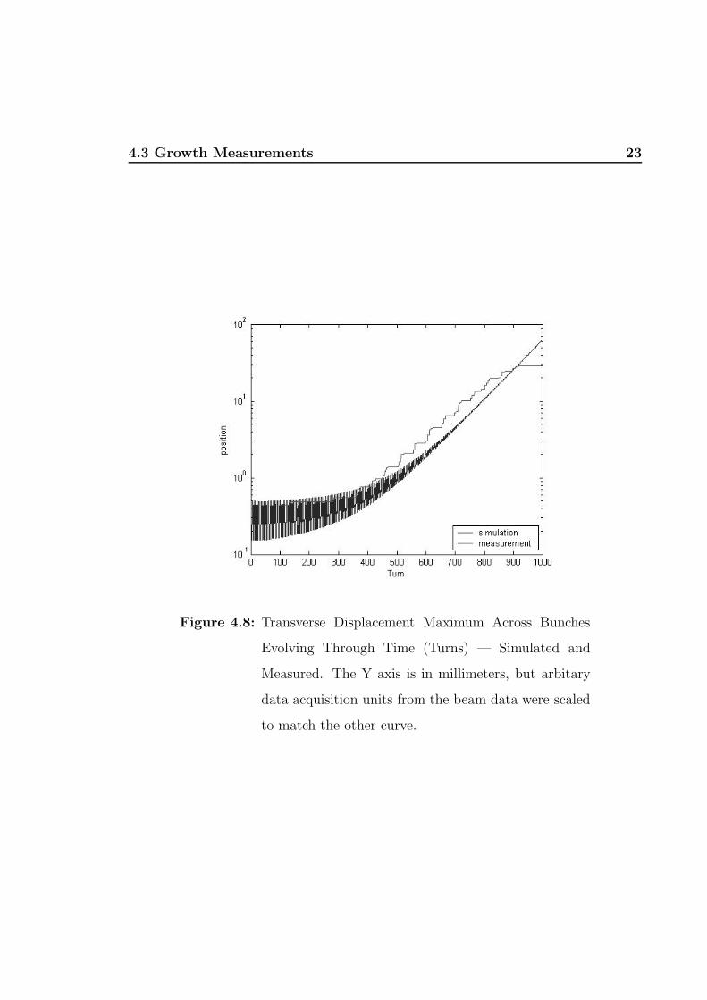
4.8 Transverse Displacement Maximum Across Bunches Evolving Through
Time (Turns) — Simulated and Measured. The Y axis is in millimeters,
but arbitary data acquisition units from the beam data were scaled to
match the other curve. . . . . . . . . . . . . . . . . . . . . . . . . . . 23
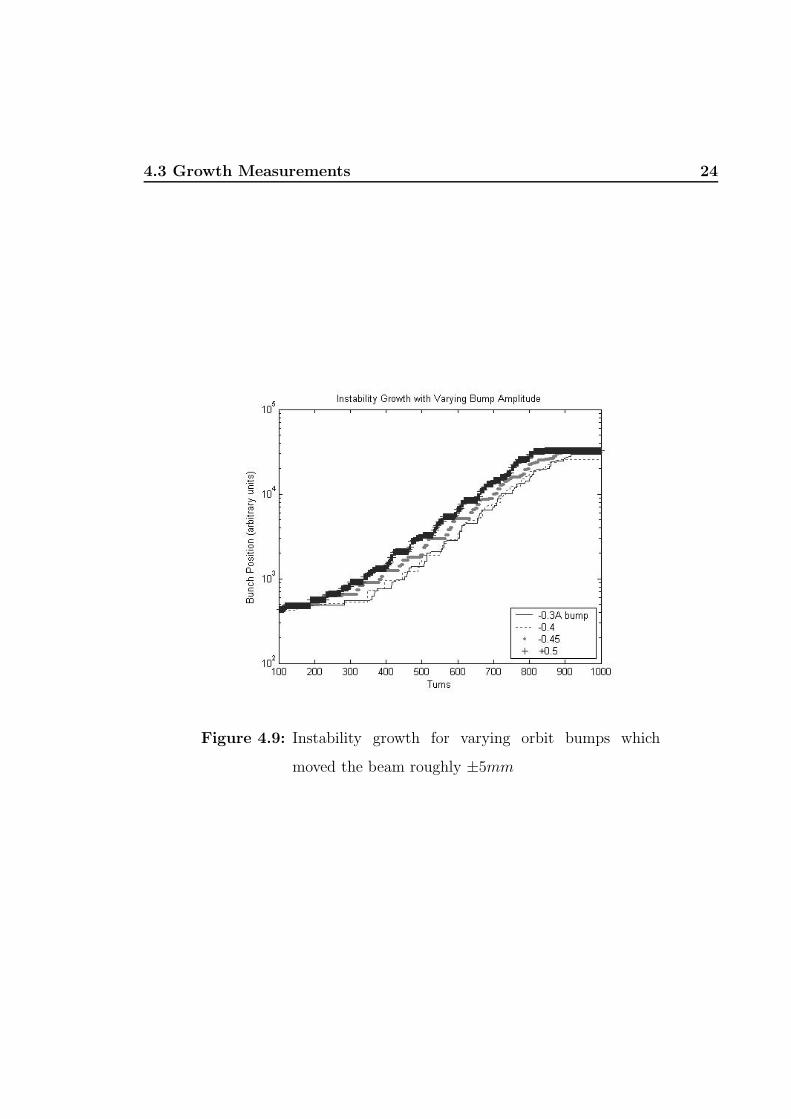
4.9 Instability growth for varying orbit bumps which moved the beam
roughly ±5mm . . . . . . . . . . . . . . . . . . . . . . . . . . . . . . 24
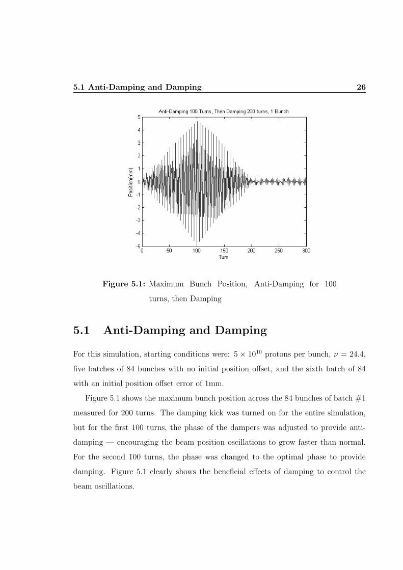
5.1 Maximum Bunch Position, Anti-Damping for 100 turns, then Damping 26
5.2 Selective Anti-Damping Time Evolution, 5 Bunches . . . . . . . . . . 28
5.3 Selective Anti-Damping, Bunch Positions after 200 turns, same data
as the previous figure . . . . . . . . . . . . . . . . . . . . . . . . . . . 29
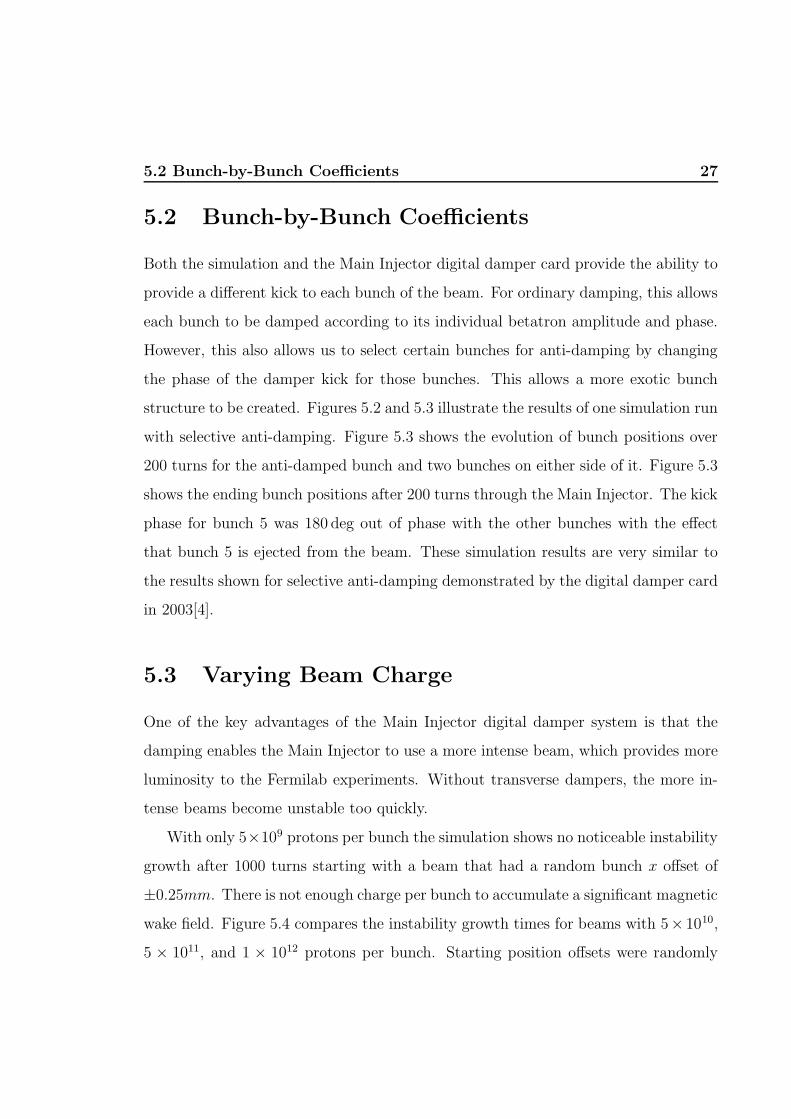
5.4 Instability Growth with Varying Bunch Intensities . . . . . . . . . . . 30
5.5 5 × 10¹¹ Protons per Bunch with Damping On and Off . . . . . . . . 31
5.6 X Dampers Off, X Instability Amplitude doubles in 144 Turns . . . . 32
5.7 Y Dampers Off, Y Instability Amplitude doubles in 83 Turns . . . . . 33
Introduction 1
Chapter 1
Introduction
In order to understand the way objects move in the real world, a beginning physics
student must move beyond ideal, frictionless approximations when calculating veloc-
ities using Newton’s laws and begin accounting for interactions with the environment
such as friction or the stretching of a rope pulling a weight. Similarly, to understand,
design, and operate synchrotron particle accelerators, one must advance beyond ideal
assumptions and calculations of beam orbits and account for interactions between the
particle beam and its environment. One such interaction comes from the conducting
walls of the accelerator beam pipe for a typical particle beam.
The interaction between the beam and beam pipe is the resistive wall effect, so
called because the beam pipe walls have a non-zero electrical resistivity. As a first
step in understanding the evolution of the resistive wall effects in a circulating beam,
this interaction has been modeled and simulated for the Fermilab Main Injector. The
results of this simulation are compared with beam measurements to gauge the utility
and correctness of the simulation and to verify explanations for behavior seen in the
beam measurements.
This simulation is only a first-step toward modeling the beam-to-environment

Introduction 2
interactions. In the Main Injector, as in all synchrotron particle accelerators, the
particles of the circulating beam are grouped into bunches, rather than having a
continuous uniform beam. The simulation presented here is a rigid bunch simulation.
“Rigid bunch” means that a bunch of particles is treated as one single lumped charge.
The simulation ignores any effects caused by having a finite sized beam with multiple
particles distributed in space. It also ignores interactions within the bunch of particles,
any space charge effects (direct EM forces between the particles in a beam), and
evolution of transverse and longitudinal bunch shape.
The following chapter of this thesis contains a brief review of some of the ac-
celerator physics concepts underlying the simulation and work. Chapter 3 discusses
the facilities and equipment involved in the project and details about the simulation
setup. Chapter 4 presents some of the results of the simulation and Chapter 5 con-
tains further results related to the damping process. After that are a few concluding
remarks and an Appendix showing some of the steps taken to calibrate and verify the
correctness of the simulation.

Accelerator Physics Review 3
Chapter 2
Accelerator Physics Review
2.1 Review of Impedance
To understand the interactions between a particle beam and its environment (beam
pipe walls, accelerating cavities, baffles, etc.) it is helpful to introduce the concept of
impedance[12].
To briefly introduce impedance, it is helpful to start at Ohm’s law for DC circuits:
V = IR, where V is the voltage across a resistor, I is the current, and R is the
electrical resistance. For an AC current, the simple resistance R must be replaced by
the complex impedance, Z, which is defined as Z = R+jX where the imaginary part
X is the called the reactance. For example, in a series R, L, C electrical circuit, for a
periodic current with frequency ω the impedance is defined as Z(ω) = R + jωL− jωC
where R is the resistance, C the capacitance and L the inductance. The impedance Z
gives the relationship between the current and the electromotive force, or work done
by the electric field. The work is done in the resistive heating (RI2), changing energy
in the magnetic field of the current (LI2/2), and changing the energy of the electric
field (q2/2C).

2.2 Resistive Wall Instability 4
There is also an impedance for a circulating charged particle beam, which can be
separated into transverse and longitudinal components. In particle accelerators, the
beam is moving in a vacuum, so there is no direct resistance. However, the beam
excites electromagnetic fields which induce currents and voltages in the beam pipe
walls. A beam’s coupling impedance relates the beam current to the induced voltages
on the beam trajectory. The induced voltage is defined as the integral over all the
EM forces on the beam. A constant velocity beam moving through the beam pipe
with some transverse (perpendicular to the axis of motion) offset from the center
will experience electric forces in the direction of beam motion and magnetic forces
perpendicular to it. These parallel and perpendicular forces produce the longitudinal
and transverse impedances.
2.2 Resistive Wall Instability
As just mentioned, the circulating beam of charged particles is accompanied by elec-
tromagnetic waves. When the beam is off-center, it will induce an image current in
the walls of the beam pipe. The electromagnetic field from the walls of the beam
pipe, the wakefield, will linger after the particles causing it have passed. This induced
electromagnetic field will exert a transverse force on the subsequent particles of the
beam. These forces introduce coupling between bunches of a bunched beam and this
feedback can lead to instability. The force on the particles from the induced magnetic
fields is called the resistive wall impedance.
The transverse effects of the resistive wall impedance on a typical beam at the
Fermilab Main Injector have been simulated and several results of this simulation will
be shown in later chapters.
2.3 Betatron Motion 5
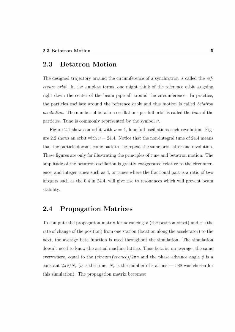
2.3 Betatron Motion
The designed trajectory around the circumference of a synchrotron is called the ref-
erence orbit. In the simplest terms, one might think of the reference orbit as going
right down the center of the beam pipe all around the circumference. In practice,
the particles oscillate around the reference orbit and this motion is called betatron
oscillation. The number of betatron oscillations per full orbit is called the tune of the
particles. Tune is commonly represented by the symbol ν.
Figure 2.1 shows an orbit with ν = 4, four full oscillations each revolution. Fig-
ure 2.2 shows an orbit with ν = 24.4. Notice that the non-integral tune of 24.4 means
that the particle doesn’t come back to the repeat the same orbit after one revolution.
These figures are only for illustrating the principles of tune and betatron motion. The
amplitude of the betatron oscillation is greatly exaggerated relative to the circumfer-
ence, and integer tunes such as 4, or tunes where the fractional part is a ratio of two
integers such as the 0.4 in 24.4, will give rise to resonances which will prevent beam
stability.
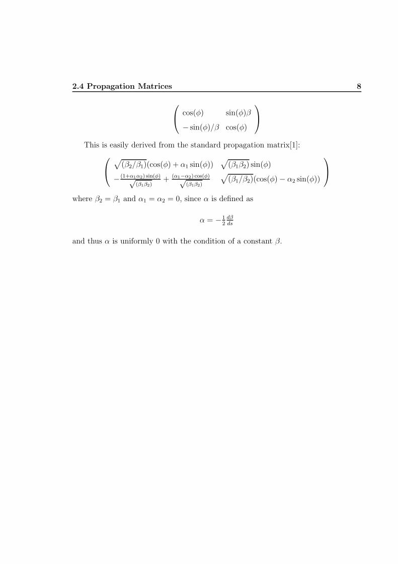
2.4 Propagation Matrices
To compute the propagation matrix for advancing x (the position offset) and x′ (the
rate of change of the position) from one station (location along the accelerator) to the
next, the average beta function is used throughout the simulation. The simulation
doesn’t need to know the actual machine lattice. Thus beta is, on average, the same
everywhere, equal to the (circumference)/2πν and the phase advance angle φ is a
constant 2πν/Ns (ν is the tune; Ns is the number of stations — 588 was chosen for
this simulation). The propagation matrix becomes:

2.4 Propagation Matrices 6
Figure 2.1: Schematic showing particle orbit with ν = 4

2.4 Propagation Matrices 7
Figure 2.2: Schematic showing particle orbit with ν = 24.4. Note
discontinuity at 0 deg due to non-integer tune value.
2.4 Propagation Matrices 8
cos(φ) sin(φ)β
− sin(φ)/β cos(φ)
This is easily derived from the standard propagation matrix[1]:
√
(β2/β1)(cos(φ) + α1 sin(φ))√
(β1β2) sin(φ)
− (1+α1α2) sin(φ)√(β1β2)
+ (α1−α2) cos(φ)√(β1β2)
√
(β1/β2)(cos(φ) − α2 sin(φ))
where β2 = β1 and α1 = α2 = 0, since α is defined as
α = −12
dβds
and thus α is uniformly 0 with the condition of a constant β.
Facilities and Experimental Equipment 9
Chapter 3
Facilities and Experimental
Equipment
This chapter describes our approach and equipment and provides some details of the
simulation implementation.
3.0.1 Fermilab Main Injector
The Fermilab Main Injector is a synchrotron approximately 3319 meters in circumfer-
ence, accelerating protons or anti-protons from 8 GeV/c to 150 GeV/c. A synchrotron
is a circular particle accelerator where the magnetic field of the steering magnets is
increased synchronously with the increase in particle energy as the particles are ac-
celerated, in order to keep the particles orbiting the accelerator ring.
The Main Injector serves as an intermediate accelerator for Fermilab’s Tevatron
and also is used in anti-proton production and fixed target experiments.
The Main Injector circulates a bunched 53 MHz beam. Thus, the time between
bunches is about 18.8ns and there are 588 buckets (bunch slots) available. (The RF
frequency times the circumference divided by c gives the number of buckets.)
Facilities and Experimental Equipment 10
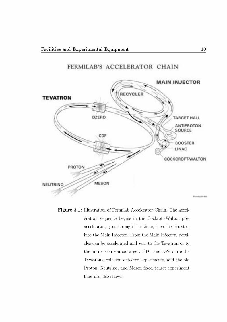
Figure 3.1: Illustration of Fermilab Accelerator Chain. The accel-
eration sequence begins in the Cockroft-Walton pre-
accelerator, goes through the Linac, then the Booster,
into the Main Injector. From the Main Injector, parti-
cles can be accelerated and sent to the Tevatron or to
the antiproton source target. CDF and DZero are the
Tevatron’s collision detector experiments, and the old
Proton, Neutrino, and Meson fixed target experiment
lines are also shown.
Facilities and Experimental Equipment 11
The Main Injector is typically filled with six separate 84-bunch batches from the
Fermilab Booster accelerator. There are two empty buckets between each batch of
84, with a longer empty space after the final batch.
The amplitudes and decay characteristics of the wake magnetic fields used in the
simulation were calculated by V. Kashikhin[6, 7] with OPERA-2D using the actual
beam pipe and laminated iron core dipole magnet geometry. The field strength results
from that modeling were then fit to a combination of two exponentials. For the
horizontal dipole moment, (the direction which will kick the beam vertically), the fit
of the Magnetic Wake Field after a dipole pulse of 1µs duration with each pole having
±1Amp at ±1mm offset from the center was found to be[3]:
B(t) = 1.612 × 10⁻⁸e(−t/49.2µs) + 3.54 × 10⁻⁹e(−t/3.45µs)
where B is given in Tesla.
The Main Injector dipole magnet beam pipe measures 6cm horizontally by 2.5cm
vertically. This ellipticity means that the magnetic field induced by a vertical offset
(the horizontal dipole field) will be greater than one caused the same offset in the
horizontal plane, and an instability induced by a vertical beam offset will grow faster
than a horizontal instability.
Unless noted otherwise, measurements and simulations in this thesis use the ver-
tical axis displacements and the above horizontal dipole as their one dimension.
3.0.2 Main Injector Transverse Dampers
The Main Injector’s transverse bunch position is detected with a stripline pickup. A
hybrid transformer’s difference output produces the position signal, which is a bipolar
signal with amplitude proportional to the bunch position. It is digitized at 212 MHz,
four times the bunch frequency, which allows the system to find the bunch phase and
amplitude[4].
Facilities and Experimental Equipment 12
Figure 3.2: Illustration of the Damper system stripline detector or
kicker.
The position detector and the damper kicker have similar stripline geometries as
depicted in Figure 3.2. Both have parallel arched plates around an inner diameter
of about 4 inches. For scale, the stripline cavity diameter is 6 inches. The kicker’s
plates are 40 inches long and each subtends 85 deg, while the pickup’s plates are 12
inches long with arcs of 110 deg[2].
The transverse signals are one set of inputs to a single board digital damping
system developed for the Fermilab Main Injector[4]. This damper board performs
all the calculations for bunch-by-bunch transverse and longitudinal beam damping.
At its heart is field-programmable gate array (FPGA) logic, outputting a digitally
synthesized damping kick to power amplifiers. The term “bunch-by-bunch” means
that the damping kick is calculated separately for each bunch. The damper card has
analog inputs for the three dimensions of beam signals, A/D converters, the DAC
output channels, and other digital inputs for beam clock and timing information.
The current transverse damper power amplifiers have enough power to induce a
0.1mm betatron oscillation in x for an 8.9 GeV/c beam. In the simulation, since the

3.1 Simulation Implementation 13
kicker is idealized at the same position as the position readout, which has the same
average beta value of roughly 26m for a typical tune around 24, this corresponds to
a kick of on the order of 4.6µrad. In the real damper system, since the kicker is at a
position with a different beta, the actual amplitude in x′ of the real kick is different.
But the simulation kick has been calibrated to have the same effect as the damper
kick.
3.1 Simulation Implementation
The simulation was implemented in Matlab, a mathematical programming language
and environment. The simulation models one transverse dimension. Matlab vectors
were constructed containing the charge, position (x), and position derivative with
respect to longitudinal position (x′ = dxds
) for each of 588 bunches. As the simulation
runs, x and x′ propagate from each station to the next.
The accelerator circumference was similarly divided into 588 equidistant locations,
or stations. The strength of the magnetic wakefield is tracked at each of those stations.
The simulation runs by taking discrete time steps, the time it takes for each bunch
to advance from one station to the next. This is simply the circumference divided by
the number of stations (588) divided by βc, the speed of the beam, or approximately
18.8ns (which is, of course, the same as the bunch spacing).
In each time step, the simulation performs the following calculations:
1. The position of the bunch at the damper readout location is recorded.
2. The kick for the bunch at the damper kick location is calculated.
3. If damping is active, the bunch at the damper kick location receives the calcu-
lated kick in x′.

3.2 Beam Pipe Diameter 14
4. Each bunch gets kick in x′ from its current station’s magnetic wakefield
5. The magnetic field at each station decays
6. Each bunch deposits wake field at each station proportional to the bunch’s
charge and position
7. x and x′ of each bunch propagate to the next station
8. The bunches (with their charge, x and x′) advance in Z to the next stations
9. Time elapses
After each full turn (588 steps), the end-of-turn bunch positions are recorded in a
vector for a time history of the beam evolution, and various maxima can be computed
to show evolution of the beam as a whole.
3.2 Beam Pipe Diameter
The Main Injector beam pipe width only produces noticeable wakefield effects in the
dipole magnets. In other parts of the circumference, the aperture is wide enough
that any wakefield effects are negligible. Approximately 75% of the circumference
has of the narrower diameter pipe. To simulate this, I use a “mask” vector with
each element corresponding to one station, and for stations where that mask is 0, no
wakefield deposition or kick occurs. 25% of the diameter of the Main Injector is thus
masked off so that there are no wakefield effects.
The magnetic wake field is divided into two parts because the computed model
indicates that the field is the sum of two separate exponential decays. Thus, the
decays are computed separately, and the field which kicks the beam is the sum of the
two parts.

Simulation Results And Experimental Data 15
Chapter 4
Simulation Results And
Experimental Data
This chapter presents some of the results from the simulation.
4.1 Instability Growth
Figures 4.1 through 4.4 show the progression of the growth of a resistive wall insta-
bility using very simple input parameters for illustration purposes. Figure 4.1 shows
the initial conditions. Six batches of 84 bunches each are set into the simulation. The
first five batches all have ideal x = 0 positions. To simulate an injection error, the
sixth batch has an x offset of 1mm. The bunch charge is identical for all bunches,
corresponding to 5×10¹⁰ protons per bunch. After 100 turns, as shown in Figure 4.2,
the effects of the injection error have begun to spread, and the betatron motion has
begun to become apparent. The instability continues to grow, and as Figure 4.4
shows, it quickly blows up the whole beam.

4.1 Instability Growth 16
Figure 4.1: Initial Conditions for Instability Growth Demonstra-
tion. One batch has a 1mm position offset. All bunches
have equal charges.

4.1 Instability Growth 17
Figure 4.2: Bunch Positions after 100 Turn Simulation
Figure 4.3: Bunch Positions after 200 Turn Simulation

4.2 Instability Growth Compared with Measurements 18
Figure 4.4: Bunch Positions after 700 Turn Simulation
4.2 Instability Growth Compared with Measure-
ments
The simulation data was analyzed to measure the growth times of the instability.
These measurements are compared with analysis of real Main Injector beam mea-
surements which were also unstable.
4.3 Growth Measurements
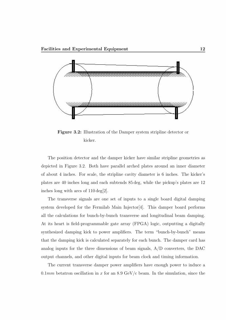
Data to measure the instability growth time was acquired with the Main Injector
digital damper system with the dampers off. All measurements are taken at a fixed,
non-accelerating, beam energy. A sample of beam positions for some bunches in the
same batch, is shown in Figure 4.5. In that figure, the position of each bunch is shown

4.3 Growth Measurements 19
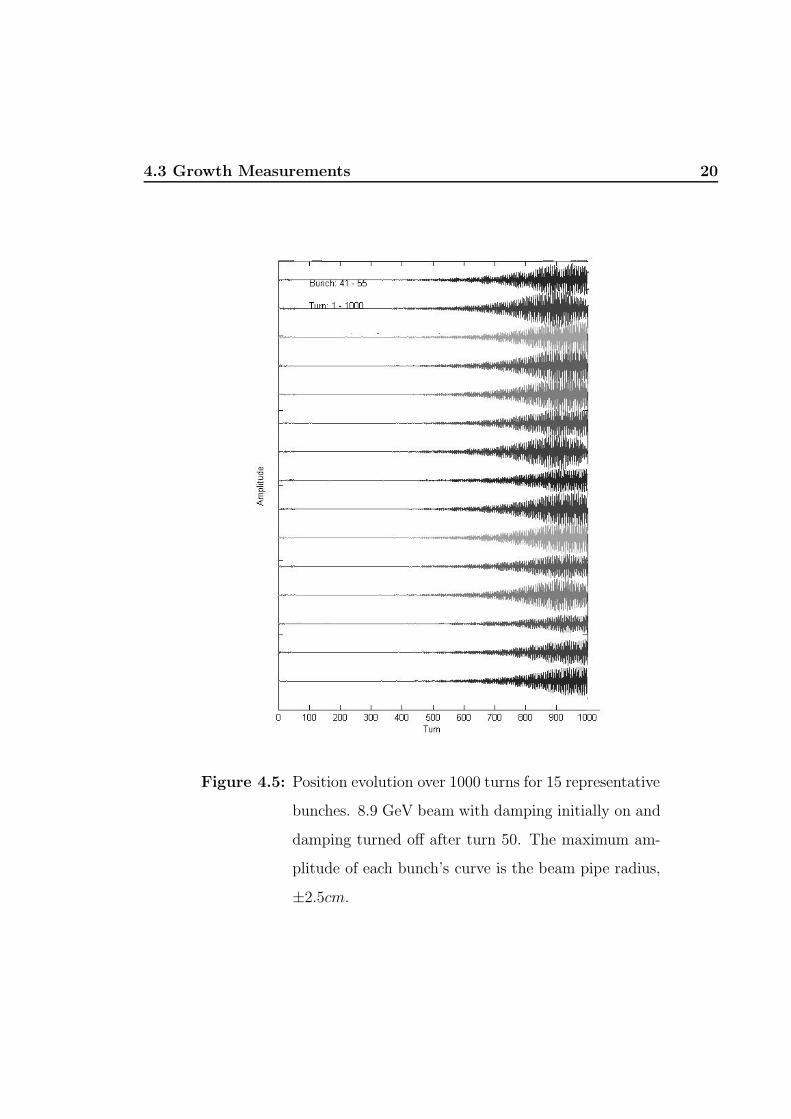
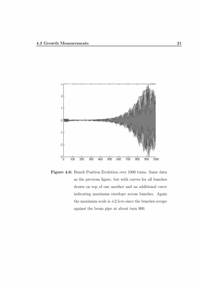
as a separate trace. In Figure 4.6 the same data is shown with each trace plotted over
the top of the others for 33 bunches. For analysis the maximum envelope across these
33 bunches is used as the indicator of the rise time of the instability. This maximum
envelope is also shown in Figure 4.6. The maximum of the beam positions also plainly
shows the point at which the beam starts scraping against the beam pipe, after about
900 turns.
The transverse dampers had been active during this experiment, and the dampers
were turned off at turn number 50, relative to the start of this plot.
Figure 4.7 shows the initial conditions for the simulated beam. Five batches have
no mean offset error, and the sixth batch of 84 bunches has a mean offset of 1mm. All
the bunches have an initial random distribution of ±0.5mm position. All the bunches
an initial x′ of zero and a charge of 5 × 10¹⁰ protons per bunch.
Figure 4.8 shows the end results of the simulation compared with the measured
beam data. The Y axis shows logarithmic scaling here. The curve which is broader
near Turn 0 is the simulated data. The “measurement” curve shows the maximum
position envelope across the bunches in the same batch as described earlier. The
“simulation” curve is created by taking the maximum position across all 84 bunches
in batch 1. Both curves are then plotted as a function of turn number.
The two curves of Figure 4.8 are quite similar, neglecting the part of the measured
curve after the beam starts physically scraping against its beam pipe around turn 900.
Each curve from Figure 4.8 was fit to an exponential function. Only the data
between turns 300 and 800 was used, in order to avoid the beam scraping in the later
turns and the earlier turns where the instability was still developing.
The results of the fit confirm the similarity in slope seen in Figure 4.8. The
simulated data was proportional to e0.0071t and the measured data rose proportional
to e0.0073t.
For this experiment, a time bump was added to the beam trajectory near one of
4.3 Growth Measurements 20
Figure 4.5: Position evolution over 1000 turns for 15 representative
bunches. 8.9 GeV beam with damping initially on and
damping turned off after turn 50. The maximum am-
plitude of each bunch’s curve is the beam pipe radius,
±2.5cm.
4.3 Growth Measurements 21
Figure 4.6: Bunch Position Evolution over 1000 turns. Same data
as the previous figure, but with curves for all bunches
drawn on top of one another and an additional curve
indicating maximum envelope across bunches. Again
the maximum scale is ±2.5cm since the bunches scrape
against the beam pipe at about turn 900.

4.3 Growth Measurements 22
Figure 4.7: Initial Bunch Positions For Simulation
the Main Injector Lambertson magnets to test any effect of moving the beam near the
septum. Bumps were tried of amplitude −.3,−0, 4,−0.45, and +.5 Amps of current
to the corrector magnets, corresponding to motions of roughly 3, 4, and 5 mm toward
the septum and 5mm away from the septum relative to the nominal beam position.
These changes did not appear to make any significant difference in the instability
growth. These amplitudes were enough to move the beam significantly but retained
a safety margin so as to not scrape the beam into the magnet septum. The variations
in these bumps and the corresponding proximity to the septum did not have any
appreciable effect on the growth time of the instability. This is shown in the log plots
of Figure 4.9. Fitting the rise times to an exponential showed that all four curves
rose proportional to between e0.0071t and e0.0073t. This means the amplitude of the
instability doubles about every 97 turns, by solving x2
x1= 2 = e0.0071t2
e0.0071t1for t2 − t1.
4.3 Growth Measurements 23
Figure 4.8: Transverse Displacement Maximum Across Bunches
Evolving Through Time (Turns) — Simulated and
Measured. The Y axis is in millimeters, but arbitary
data acquisition units from the beam data were scaled
to match the other curve.
4.3 Growth Measurements 24
Figure 4.9: Instability growth for varying orbit bumps which
moved the beam roughly ±5mm

Damping 25
Chapter 5
Damping
As indicated previously, the simulation includes simulation of a damping kick which
can produce a 0.1mm transverse displacement after a quarter of a betatron oscillation.
The position for the kick is sensed at one position and the kick is applied at one
position. For the purposes of these simulations, the readout and kick position are
the same, although in practice, they are not at the exact same location. The same
algorithm that is used in the FPGA for calculating the damping kick is used in the
simulation. This includes a calculation of the bunch motion phase.
Consider the analogy of a person on a swing. If you push them forward while
they are still in the backwards motion part of the swing, that will lessen the height of
their swing. Conversely, if you push them forwards while they are moving forwards,
an in-phase push, then you will increase the height of their swing.
The same principles apply with beam damping. Applying a kick out-of-phase
with the particle oscillations will diminish the amplitude of the oscillation. This is
the damping process. Applying a kick in-phase with the particle motion will increase
the oscillation amplitude of the particle, and this is anti-damping, or pinging, the
beam.
5.1 Anti-Damping and Damping 26
Figure 5.1: Maximum Bunch Position, Anti-Damping for 100
turns, then Damping
5.1 Anti-Damping and Damping
For this simulation, starting conditions were: 5 × 10¹⁰ protons per bunch, ν = 24.4,
five batches of 84 bunches with no initial position offset, and the sixth batch of 84
with an initial position offset error of 1mm.
Figure 5.1 shows the maximum bunch position across the 84 bunches of batch #1
measured for 200 turns. The damping kick was turned on for the entire simulation,
but for the first 100 turns, the phase of the dampers was adjusted to provide anti-
damping — encouraging the beam position oscillations to grow faster than normal.
For the second 100 turns, the phase was changed to the optimal phase to provide
damping. Figure 5.1 clearly shows the beneficial effects of damping to control the
beam oscillations.
5.2 Bunch-by-Bunch Coefficients 27
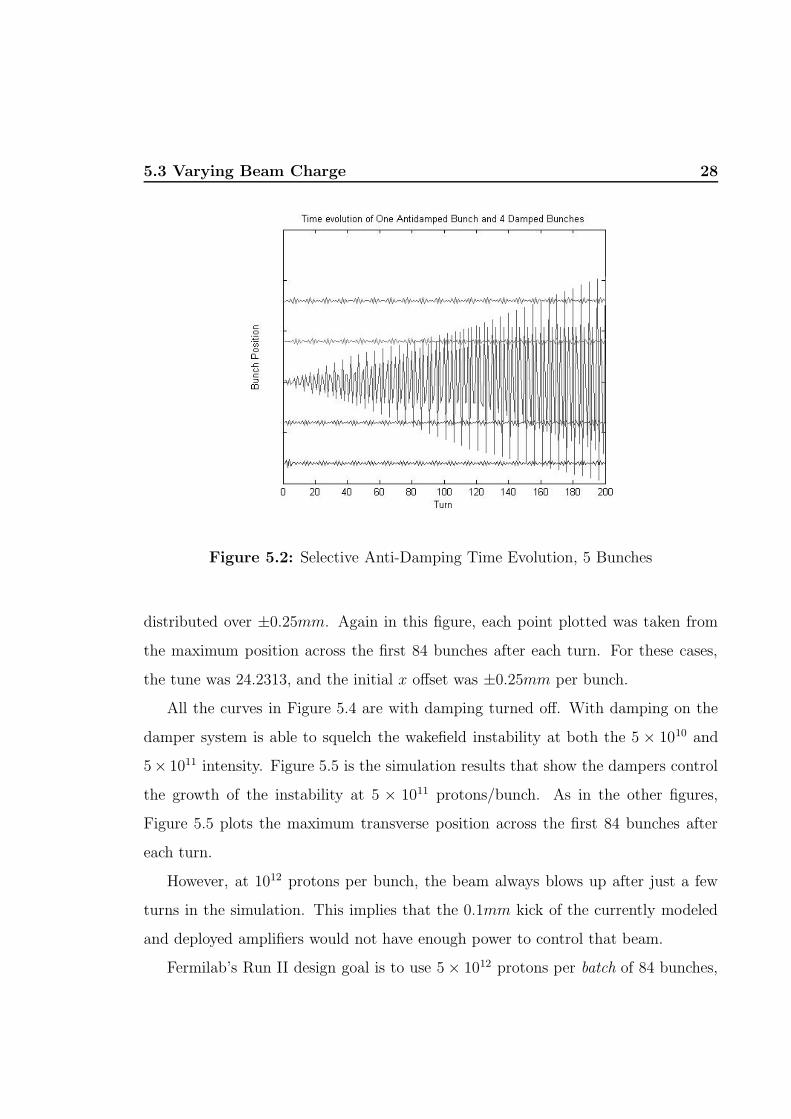
5.2 Bunch-by-Bunch Coefficients
Both the simulation and the Main Injector digital damper card provide the ability to
provide a different kick to each bunch of the beam. For ordinary damping, this allows
each bunch to be damped according to its individual betatron amplitude and phase.
However, this also allows us to select certain bunches for anti-damping by changing
the phase of the damper kick for those bunches. This allows a more exotic bunch
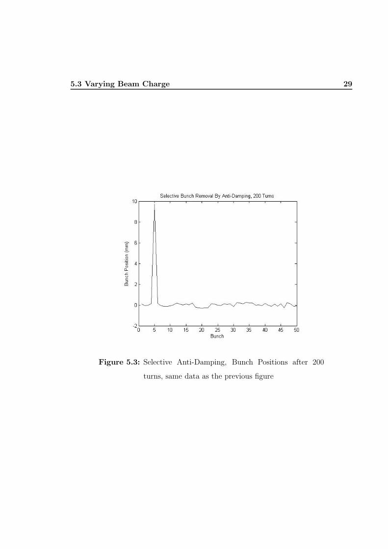
structure to be created. Figures 5.2 and 5.3 illustrate the results of one simulation run
with selective anti-damping. Figure 5.3 shows the evolution of bunch positions over
200 turns for the anti-damped bunch and two bunches on either side of it. Figure 5.3
shows the ending bunch positions after 200 turns through the Main Injector. The kick
phase for bunch 5 was 180 deg out of phase with the other bunches with the effect
that bunch 5 is ejected from the beam. These simulation results are very similar to
the results shown for selective anti-damping demonstrated by the digital damper card
in 2003[4].
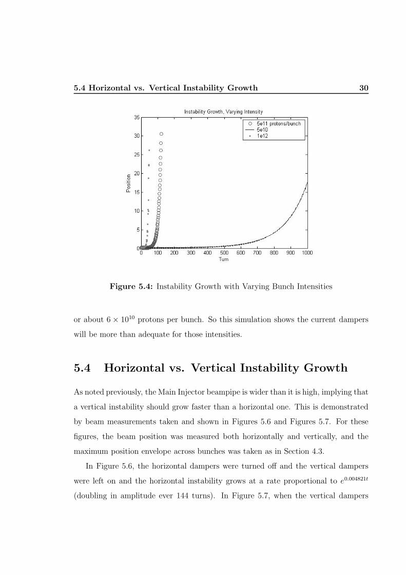
5.3 Varying Beam Charge
One of the key advantages of the Main Injector digital damper system is that the
damping enables the Main Injector to use a more intense beam, which provides more
luminosity to the Fermilab experiments. Without transverse dampers, the more in-
tense beams become unstable too quickly.
With only 5×10⁹ protons per bunch the simulation shows no noticeable instability
growth after 1000 turns starting with a beam that had a random bunch x offset of
±0.25mm. There is not enough charge per bunch to accumulate a significant magnetic
wake field. Figure 5.4 compares the instability growth times for beams with 5× 10¹⁰,
5 × 10¹¹, and 1 × 10¹² protons per bunch. Starting position offsets were randomly
5.3 Varying Beam Charge 28
Figure 5.2: Selective Anti-Damping Time Evolution, 5 Bunches
distributed over ±0.25mm. Again in this figure, each point plotted was taken from
the maximum position across the first 84 bunches after each turn. For these cases,
the tune was 24.2313, and the initial x offset was ±0.25mm per bunch.
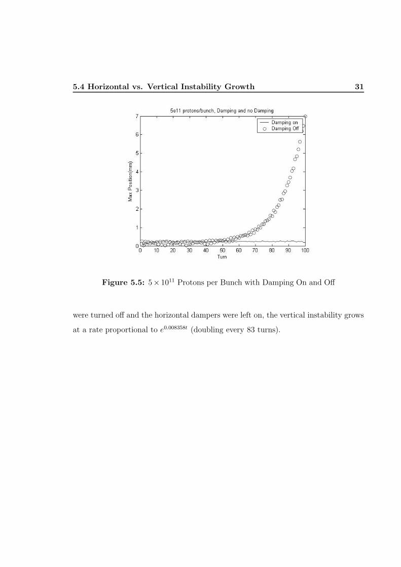
All the curves in Figure 5.4 are with damping turned off. With damping on the
damper system is able to squelch the wakefield instability at both the 5 × 10¹⁰ and
5× 10¹¹ intensity. Figure 5.5 is the simulation results that show the dampers control
the growth of the instability at 5 × 10¹¹ protons/bunch. As in the other figures,
Figure 5.5 plots the maximum transverse position across the first 84 bunches after
each turn.
However, at 1012 protons per bunch, the beam always blows up after just a few
turns in the simulation. This implies that the 0.1mm kick of the currently modeled
and deployed amplifiers would not have enough power to control that beam.
Fermilab’s Run II design goal is to use 5 × 10¹² protons per batch of 84 bunches,
5.3 Varying Beam Charge 29
Figure 5.3: Selective Anti-Damping, Bunch Positions after 200
turns, same data as the previous figure
5.4 Horizontal vs. Vertical Instability Growth 30
Figure 5.4: Instability Growth with Varying Bunch Intensities
or about 6 × 10¹⁰ protons per bunch. So this simulation shows the current dampers
will be more than adequate for those intensities.
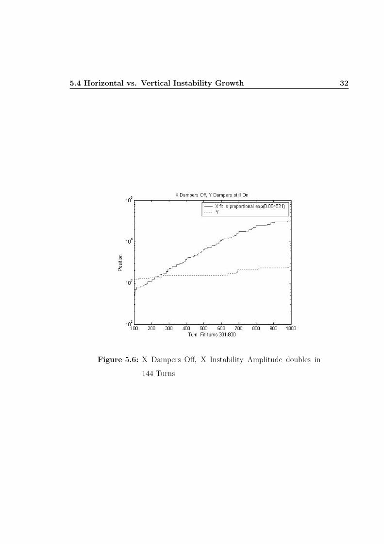
5.4 Horizontal vs. Vertical Instability Growth
As noted previously, the Main Injector beampipe is wider than it is high, implying that
a vertical instability should grow faster than a horizontal one. This is demonstrated
by beam measurements taken and shown in Figures 5.6 and Figures 5.7. For these
figures, the beam position was measured both horizontally and vertically, and the
maximum position envelope across bunches was taken as in Section 4.3.
In Figure 5.6, the horizontal dampers were turned off and the vertical dampers
were left on and the horizontal instability grows at a rate proportional to e0.004821t
(doubling in amplitude ever 144 turns). In Figure 5.7, when the vertical dampers
5.4 Horizontal vs. Vertical Instability Growth 31
Figure 5.5: 5× 10¹¹ Protons per Bunch with Damping On and Off
were turned off and the horizontal dampers were left on, the vertical instability grows
at a rate proportional to e0.008358t (doubling every 83 turns).
5.4 Horizontal vs. Vertical Instability Growth 32
Figure 5.6: X Dampers Off, X Instability Amplitude doubles in
144 Turns
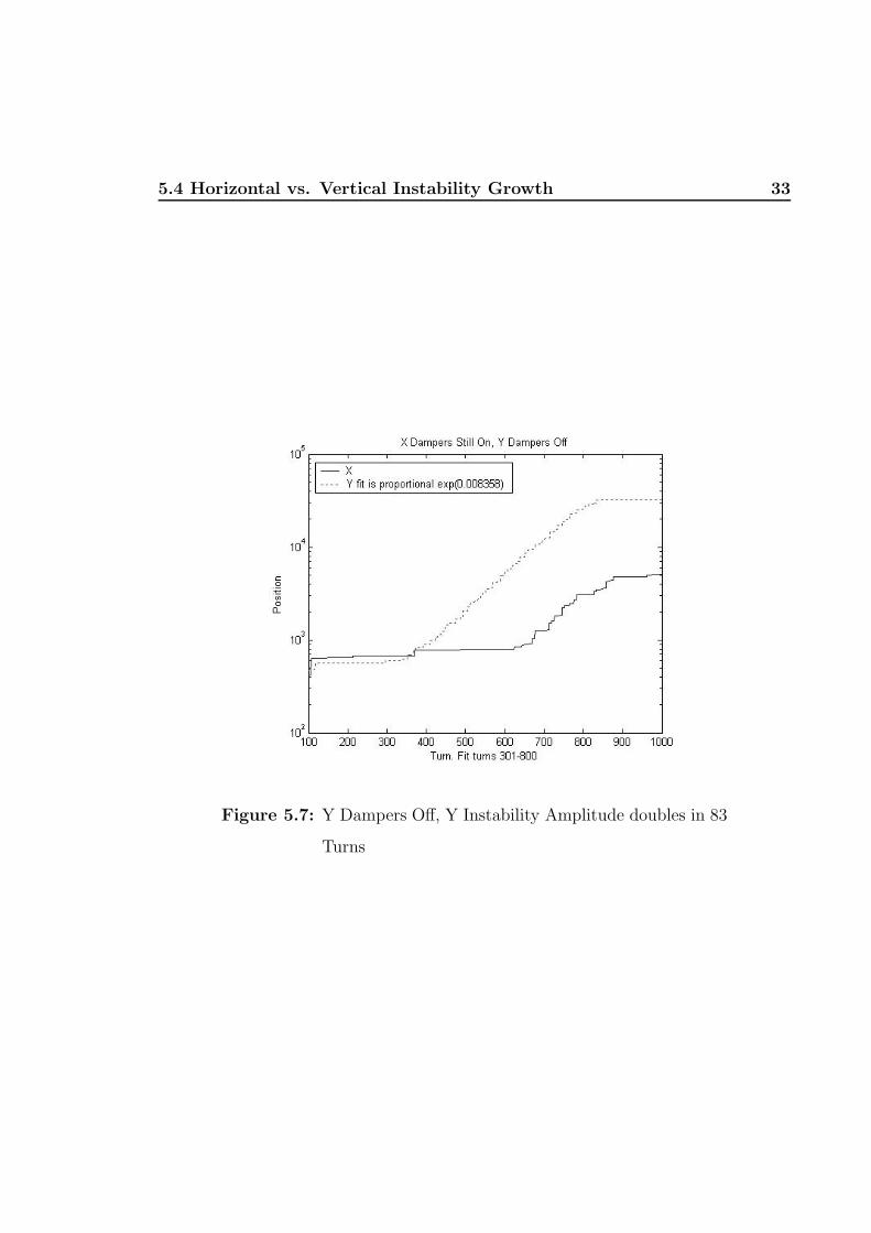
5.4 Horizontal vs. Vertical Instability Growth 33
Figure 5.7: Y Dampers Off, Y Instability Amplitude doubles in 83
Turns

Conclusions 34
Chapter 6
Conclusions
This rigid bunch simulation has proven to be a useful tool for understanding the
behavior of the beam in the Fermilab Main Injector. The simulation also is a useful
aid to understanding the Main Injector digital bunch-by-bunch damper card, the need
for such damping, its performance, and its capabilities.
Use of a rigid bunch approximation is one limitation to this simulation. Use
of rigid bunches does not allow it to account for finite chromaticity which spreads
the frequencies of the orbiting particles and can wash out the growth of wakefield
instabilities. This property is used to allow the Main Injector to function at relatively
high intensities without any damping. However, to go to desired higher intensities,
damping is needed. Another limitation is that the beam positions are allowed to go
to infinity rather than being clipped at the diameter of the beam pipe where the
particles would be scraped away. This last limitation would be a straightforward
change to the simulation code.

Simulation Calibration Procedures 35
Appendix A
Simulation Calibration Procedures
To demonstrate that the basics of the calibration were correct, some simple operations
were performed which could be compared with easily computed expected values. This
appendix contains a list of those checks.
1. The transfer matrix which advances x and x′ from one station to the next was
checked. For this check, x and x′ are set to a set of simple patterns, for instance
x = 0, x′ = 1, and the system is advanced to the next station. We were able to
easily check that the values at the next station were correct.
2. After integral number of tunes, the beam x and x′ are back where they started.
To show this, an initial pattern was set for the bunches in x and x′, the wakefield
deposition, decay, and kick were turned off, and the beam was put through a
number of turns N so that Nν is an integer. For instance, with the beam tune
ν = 24.4, the bunches are advanced through 5 turns, and the resulting x and x′
was observed to be the same as the initial conditions.
3. The value of the magnetic wakefield was compared with its expected value.
This was done by setting the number of particles in a bunch to 1.2 × 10¹³ to
Simulation Calibration Procedures 36
get 2µC per bunch, then observing that the induced magneting field matched
the amplitude predicted by the input model. The magnetic field made to decay
for lengths of time and the amplitude in the simulation matched the predicted
values.
4. With a starting condition of one bunch stepped around the ring, the simulation
produced the expected betatron oscillation pattern.
5. The Fermilab Main Injector transverse damper power amplifiers have enough
power to induce a 0.1mm kick to the beam. To verify the simulation had the
correct damper kick strength, all the charge deposition, decay, and resistive-
wall kick features were turned off, and one bunch was kicked by the damper one
time. After one-quarter period of betatron oscillation, the bunch is observed to
have the expected 0.1mm betatron oscillation amplitude.

BIBLIOGRAPHY 37
Bibliography
[1] D. A. Edwards and M. J. Syphers, An Introduction to the Physiscs of High
Energy Accelerators John Wiley & Sons, New York, 1993.
[2] Fermilab Technical Drawing Numbers 0430.030-MD-260677 and 0430.030-MD-
260687 for Kicker and Detector Striplines.
[3] G. William Foster, Wake Field Excel Spreadsheet Unpublished excel file, 2003.
[4] G. William Foster, Sten Hansen, Dennis Nicklaus, Warren Schappert, Alexei
Seminov, Dave Wildman, and W. Ashmanskas, Bunch-By-Bunch Digital
Dampers for the Fermilab Main Injector and Recycler Particle Accelerator Con-
ference, 2003
[5] Gerald P. Jackson, The Effect of Chromatic Decoherence on Transverse Injection
Oscillation Damping Published Proceedings of Technical Workshop on Feedback
Control of Multi-Bunch Instabilities in Proton Colliders at the Highest Energies
and Luminosities, Erice, Sicily, 1992. Fermilab Document Fermilab-Conf-93/010.
[6] V. S. Kashikhin, Wake Magnetic Field Analysis. Unpublished memo, May 30,
2003.
[7] V. S. Kashikhin, Wake Magnetic Field Analysis. Unpublished memo including
Vertical Dipole Field and Horizontal Dipole Field, Feb. 27, 2004.
BIBLIOGRAPHY 38
[8] S. Koscielniak and H. J. Tran, Properties of a Transverse Damping System,
Calculated by a Simple Matrix Formalism. Proceedings of the 1995 IEEE Particle
Accelerator Conference, Dallas Texas, May 1-5 1995.
[9] S. Y. Lee, Accelerator Physics. World Scientific Publishing Co., Singapore, 1999.
[10] C. Y. Tan and J. Steimel, The Tevatron Transverse Dampers. In Proceedings of
the 2003 Particle Acclerator Conference, Portland, OR, 2003.
[11] C. S. Taylor Microwave Kickers and Pickups in Oxford 1991, Proceedings, RF
engineering for particle accelerators, vol. 2, 458-473. CERN Geneva - CERN-92-
03.x
[12] Bruno W. Zotter and Semyon A. Kheifets, Impedances and Wakes in High-Energy
Particle Accelerators. World Scientific Publishing Co., Singapore, 1998.
[13] V.M. Zhabitsky, Transverse Feedback System with a Digital Filter and Additional
Delay, Proceedings of the 1986 European Particle Accelerator Conference, p.
1833, 1986.
Recommended