Should Unconventional Monetary Policies Become Conventional? Dominic Quint and Pau Rabanal
Discussant: Annette Vissing-Jorgensen, University of California Berkeley and NBER
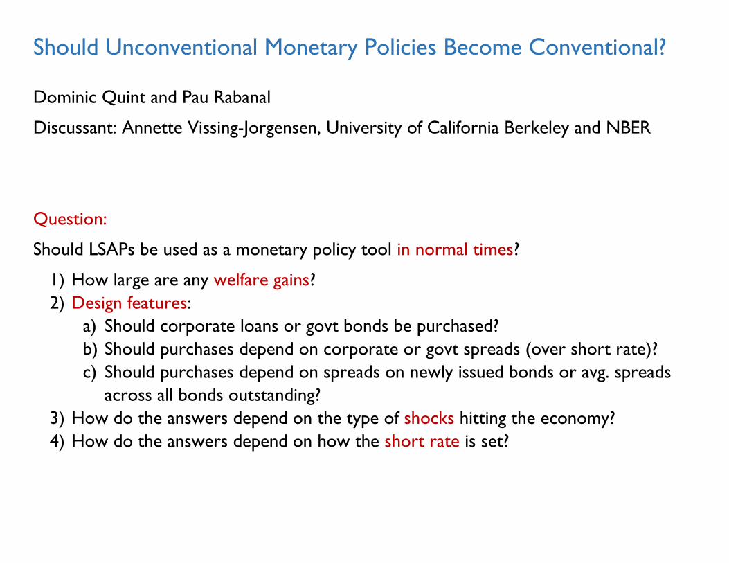
Question:
Should LSAPs be used as a monetary policy tool in normal times?
1) How large are any welfare gains?
2) Design features:
a) Should corporate loans or govt bonds be purchased?
b) Should purchases depend on corporate or govt spreads (over short rate)?
c) Should purchases depend on spreads on newly issued bonds or avg. spreads
across all bonds outstanding?
3) How do the answers depend on the type of shocks hitting the economy?
4) How do the answers depend on how the short rate is set?
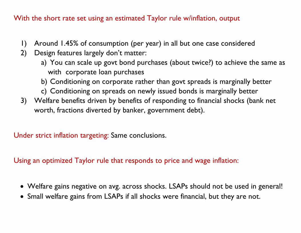
With the short rate set using an estimated Taylor rule w/inflation, output
1) Around 1.45% of consumption (per year) in all but one case considered
2) Design features largely don’t matter:
a) You can scale up govt bond purchases (about twice?) to achieve the same as
with corporate loan purchases
b) Conditioning on corporate rather than govt spreads is marginally better
c) Conditioning on spreads on newly issued bonds is marginally better
3) Welfare benefits driven by benefits of responding to financial shocks (bank net
worth, fractions diverted by banker, government debt).
Under strict inflation targeting: Same conclusions.
Using an optimized Taylor rule that responds to price and wage inflation:
Welfare gains negative on avg. across shocks. LSAPs should not be used in general!
Small welfare gains from LSAPs if all shocks were financial, but they are not.
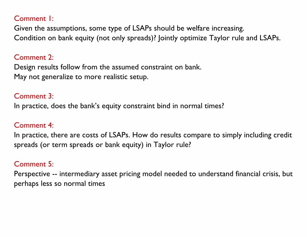
Comment 1:
Given the assumptions, some type of LSAPs should be welfare increasing.
Condition on bank equity (not only spreads)? Jointly optimize Taylor rule and LSAPs.
Comment 2:
Design results follow from the assumed constraint on bank.
May not generalize to more realistic setup.
Comment 3:
In practice, does the bank’s equity constraint bind in normal times?
Comment 4:
In practice, there are costs of LSAPs. How do results compare to simply including credit
spreads (or term spreads or bank equity) in Taylor rule?
Comment 5:
Perspective -- intermediary asset pricing model needed to understand financial crisis, but
perhaps less so normal times
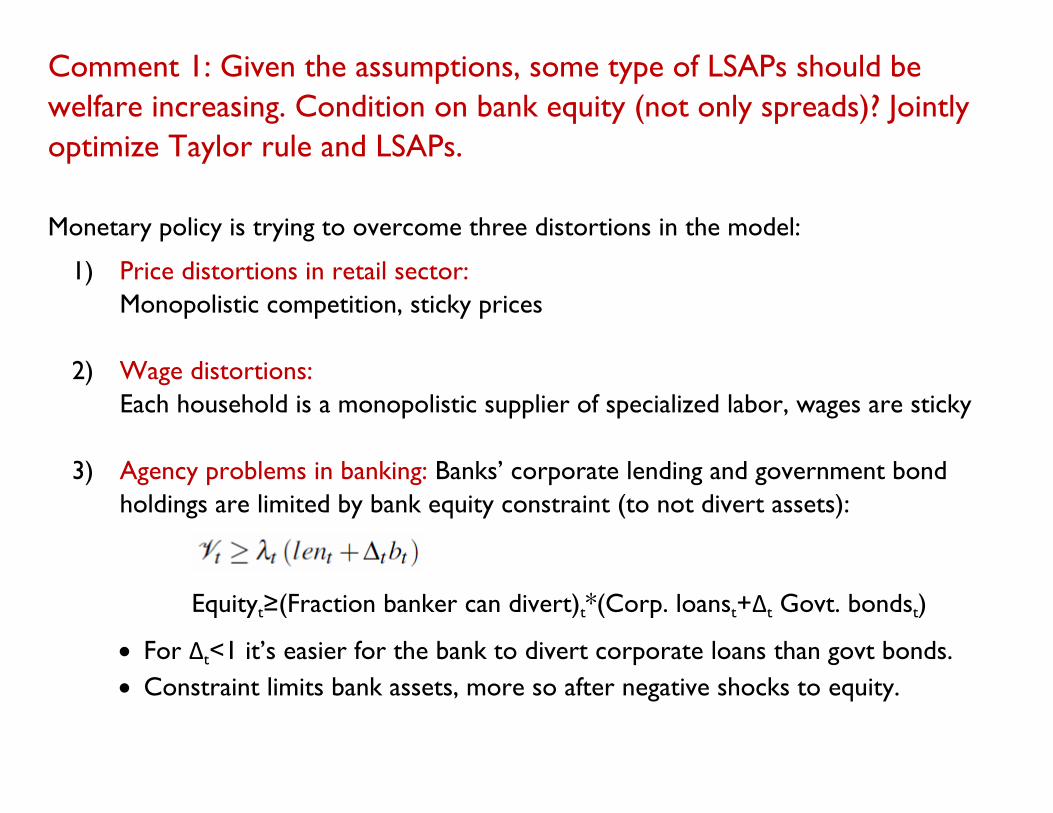
Comment 1: Given the assumptions, some type of LSAPs should be
welfare increasing. Condition on bank equity (not only spreads)? Jointly
optimize Taylor rule and LSAPs.
Monetary policy is trying to overcome three distortions in the model:
1) Price distortions in retail sector:
Monopolistic competition, sticky prices
2) Wage distortions:
Each household is a monopolistic supplier of specialized labor, wages are sticky
3) Agency problems in banking: Banks’ corporate lending and government bond
holdings are limited by bank equity constraint (to not divert assets):
Equityt≥(Fraction banker can divert)t*(Corp. loanst+Δt Govt. bondst)
For Δt<1 it’s easier for the bank to divert corporate loans than govt bonds.
Constraint limits bank assets, more so after negative shocks to equity.
Crucially:
Central bank (CB) not subject to the agency problem
No costs of LSAPs:
- The CB is as efficient at intermediation as banks
- No one worries about potential Fed losses
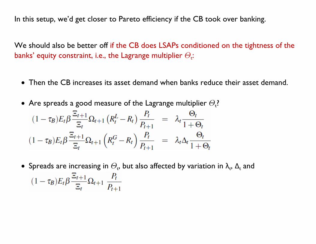
In this setup, we’d get closer to Pareto efficiency if the CB took over banking.
We should also be better off if the CB does LSAPs conditioned on the tightness of the
banks’ equity constraint, i.e., the Lagrange multiplier t:
Then the CB increases its asset demand when banks reduce their asset demand.
Are spreads a good measure of the Lagrange multiplier t?
Spreads are increasing in t, but also affected by variation in λt, Δt and
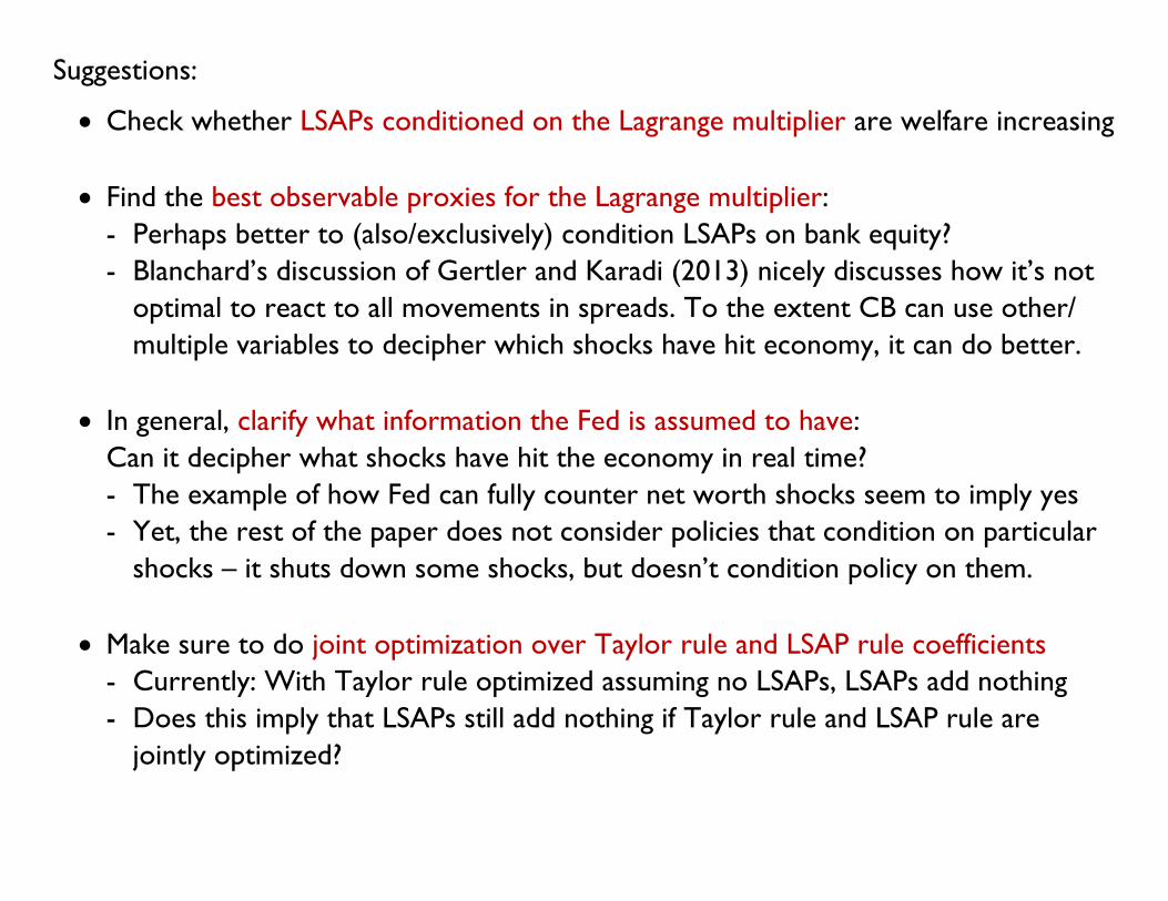
Suggestions:
Check whether LSAPs conditioned on the Lagrange multiplier are welfare increasing
Find the best observable proxies for the Lagrange multiplier:
- Perhaps better to (also/exclusively) condition LSAPs on bank equity?
- Blanchard’s discussion of Gertler and Karadi (2013) nicely discusses how it’s not
optimal to react to all movements in spreads. To the extent CB can use other/
multiple variables to decipher which shocks have hit economy, it can do better.
In general, clarify what information the Fed is assumed to have:
Can it decipher what shocks have hit the economy in real time?
- The example of how Fed can fully counter net worth shocks seem to imply yes
- Yet, the rest of the paper does not consider policies that condition on particular
shocks – it shuts down some shocks, but doesn’t condition policy on them.
Make sure to do joint optimization over Taylor rule and LSAP rule coefficients
- Currently: With Taylor rule optimized assuming no LSAPs, LSAPs add nothing
- Does this imply that LSAPs still add nothing if Taylor rule and LSAP rule are
jointly optimized?
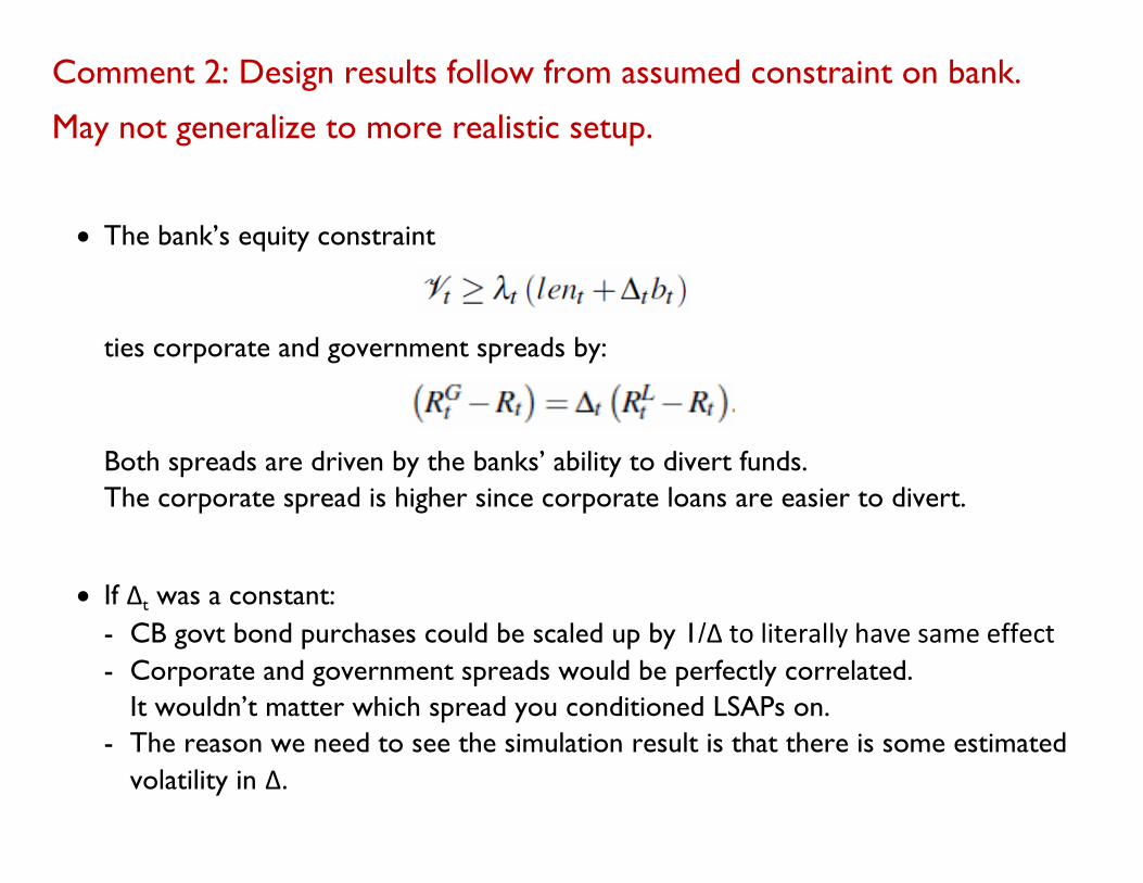
Comment 2: Design results follow from assumed constraint on bank.
May not generalize to more realistic setup.
The bank’s equity constraint
ties corporate and government spreads by:
Both spreads are driven by the banks’ ability to divert funds.
The corporate spread is higher since corporate loans are easier to divert.
If Δt was a constant:
- CB govt bond purchases could be scaled up by 1/Δ to literally have same effect
- Corporate and government spreads would be perfectly correlated.
It wouldn’t matter which spread you conditioned LSAPs on.
- The reason we need to see the simulation result is that there is some estimated
volatility in Δ.
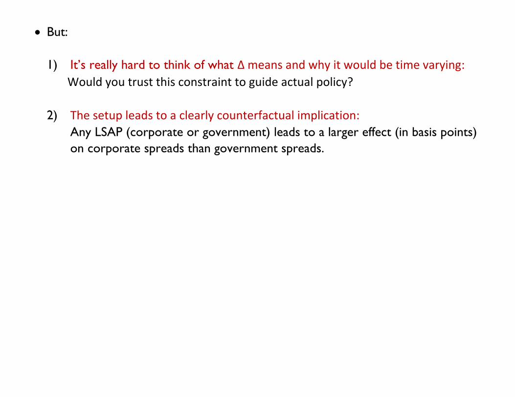
But:
1) It’s really hard to think of what Δ means and why it would be time varying:
Would you trust this constraint to guide actual policy?
2) The setup leads to a clearly counterfactual implication:
Any LSAP (corporate or government) leads to a larger effect (in basis points)
on corporate spreads than government spreads.
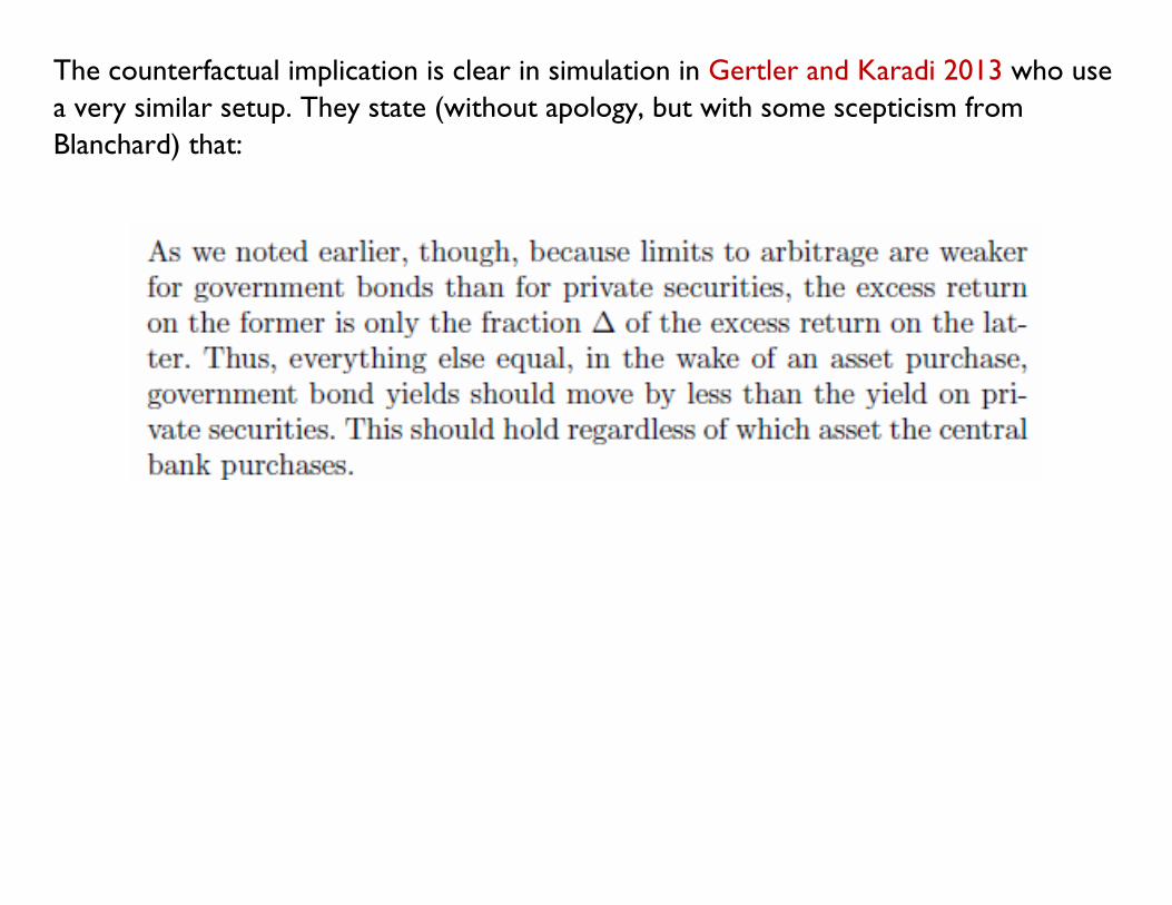
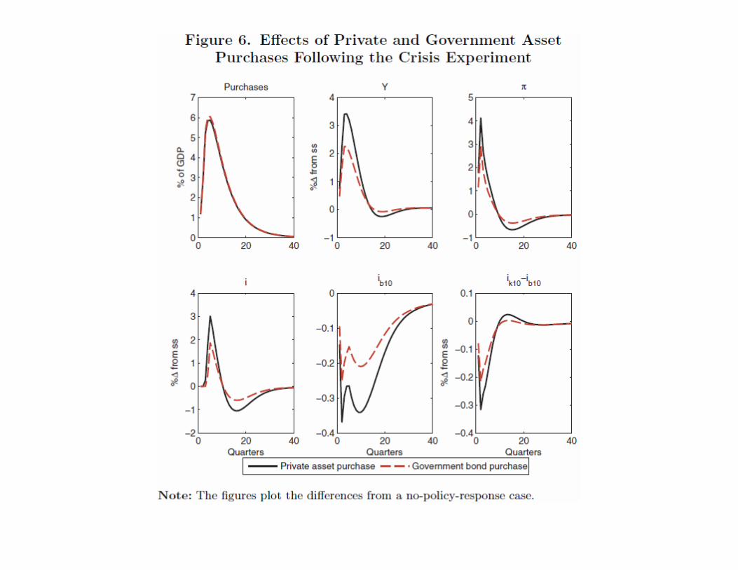
The counterfactual implication is clear in simulation in Gertler and Karadi 2013 who use
a very similar setup. They state (without apology, but with some scepticism from
Blanchard) that:
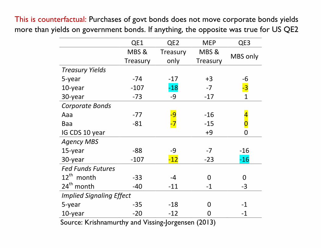
This is counterfactual: Purchases of govt bonds does not move corporate bonds yields
more than yields on government bonds. If anything, the opposite was true for US QE2
QE1 QE2 MEP QE3 MBS &
Treasury Treasury
only MBS &
Treasury MBS only
Treasury Yields 5-year -74 -17 +3 -6 10-year -107 -18 -7 -3 30-year -73 -9 -17 1 Corporate Bonds Aaa -77 -9 -16 4 Baa -81 -7 -15 0 IG CDS 10 year +9 0 Agency MBS 15-year -88 -9 -7 -16 30-year -107 -12 -23 -16 Fed Funds Futures 12th month -33 -4 0 0 24th month -40 -11 -1 -3 Implied Signaling Effect 5-year -35 -18 0 -1 10-year -20 -12 0 -1
Source: Krishnamurthy and Vissing-Jorgensen (2013)
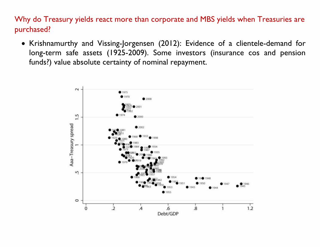
Why do Treasury yields react more than corporate and MBS yields when Treasuries are
purchased?
Krishnamurthy and Vissing-Jorgensen (2012): Evidence of a clientele-demand for
long-term safe assets (1925-2009). Some investors (insurance cos and pension
funds?) value absolute certainty of nominal repayment.
Similarly, for QE3, if current paper’s constraint is correct corporate bond yields should
probably move as much as MBS, but they didn’t
Seems more likely that MBS yields moved more in QE3 because purchases affected
the scarcity of production (current-coupon) MBS rather than generally alleviated
financial intermediaries’ equity constraint (more evidence in Krishnamurthy and
Vissing-Jorgensen (2013)).
The problem is that the model has one channel for LSAPs to work: Alleviation of the
banks’ equity constraint – a ``general” channel
That was probably important in QE1 at peak of crisis
But in normal times (QE2, QE3) ``specific” channels affecting the particular asset
class purchased may be more important (effect on price of long-term safety, effect
on scarcity of production MBS), aside from any signaling effects from QE.
The design results rely crucially on the ``general” channel and they may not carry over
to a setup that more realistically captures the channels for QE in normal times.
Comment 3: In practice, does the bank’s equity constraint bind in normal
times?
In the model the answer seems to be yes – the bank scales up operations to make
the constraint bind given equity (some discussion of this would be nice).
But in other models with equity constraints on banks, the constraint is not
necessarily binding in normal times. It only binds in crisis following bank equity
losses. Then there is no need or LSAPs in normal times (unless they work via other
channels).
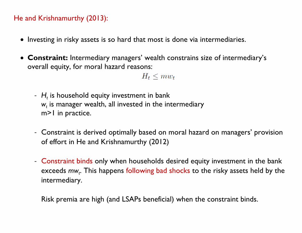
He and Krishnamurthy (2013):
Investing in risky assets is so hard that most is done via intermediaries.
Constraint: Intermediary managers’ wealth constrains size of intermediary’s
overall equity, for moral hazard reasons:
- Ht is household equity investment in bank
wt is manager wealth, all invested in the intermediary
m>1 in practice.
- Constraint is derived optimally based on moral hazard on managers’ provision
of effort in He and Krishnamurthy (2012)
- Constraint binds only when households desired equity investment in the bank
exceeds mwt. This happens following bad shocks to the risky assets held by the
intermediary.
Risk premia are high (and LSAPs beneficial) when the constraint binds.
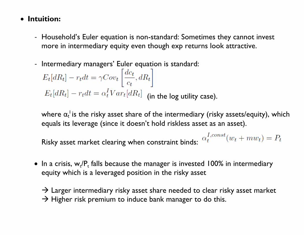
Intuition:
- Household’s Euler equation is non-standard: Sometimes they cannot invest
more in intermediary equity even though exp returns look attractive.
- Intermediary managers’ Euler equation is standard:
(in the log utility case).
where αtI is the risky asset share of the intermediary (risky assets/equity), which
equals its leverage (since it doesn’t hold riskless asset as an asset).
Risky asset market clearing when constraint binds:
In a crisis, wt/Pt falls because the manager is invested 100% in intermediary
equity which is a leveraged position in the risky asset
Larger intermediary risky asset share needed to clear risky asset market
Higher risk premium to induce bank manager to do this.
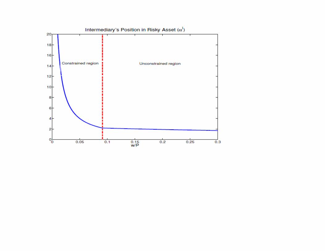
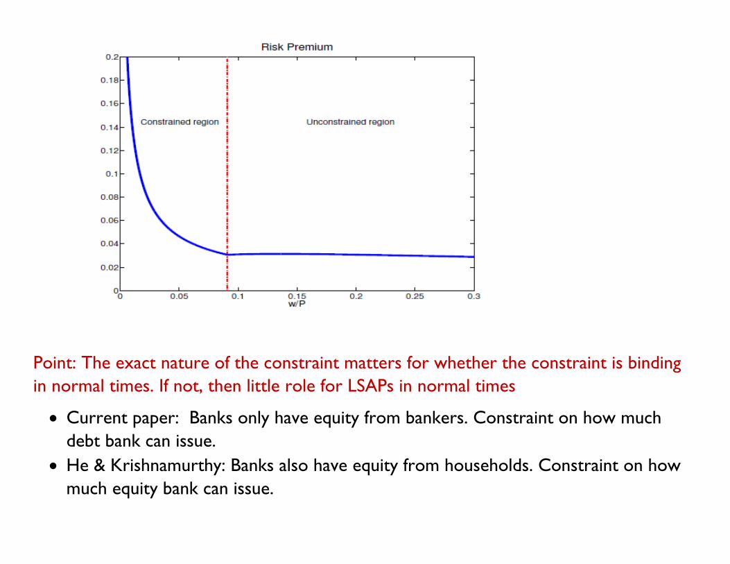
Point: The exact nature of the constraint matters for whether the constraint is binding
in normal times. If not, then little role for LSAPs in normal times
Current paper: Banks only have equity from bankers. Constraint on how much
debt bank can issue.
He & Krishnamurthy: Banks also have equity from households. Constraint on how
much equity bank can issue.
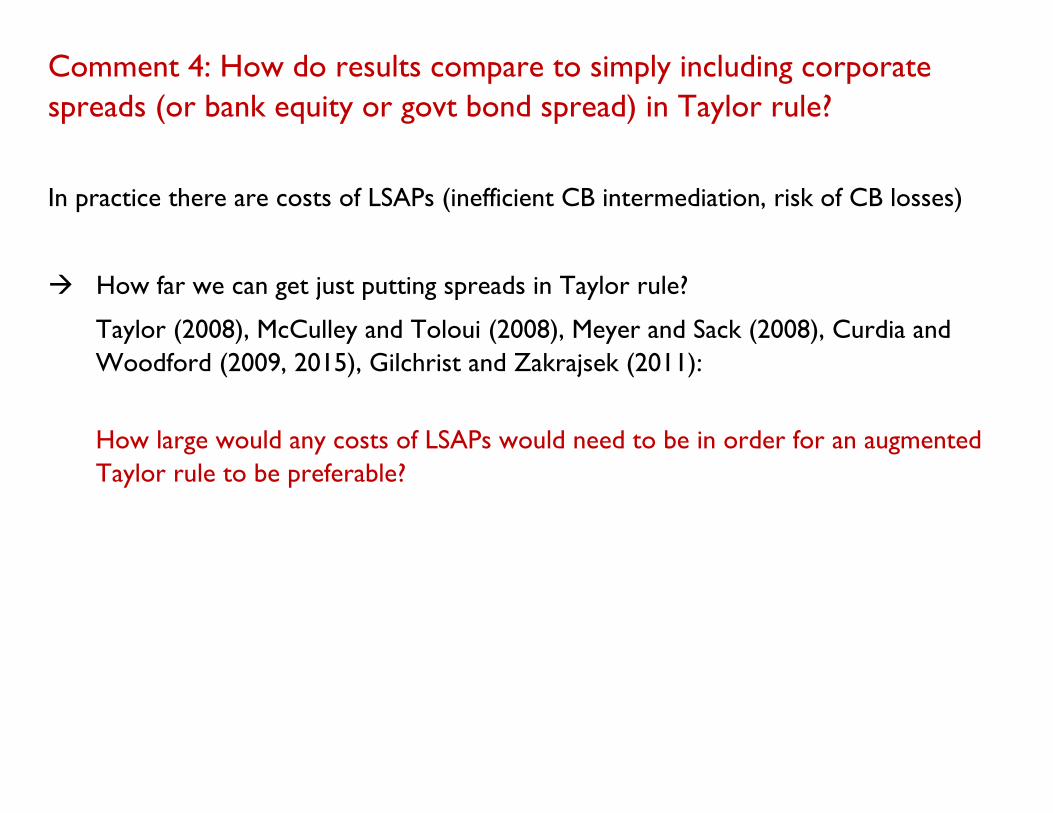
Comment 4: How do results compare to simply including corporate
spreads (or bank equity or govt bond spread) in Taylor rule?
In practice there are costs of LSAPs (inefficient CB intermediation, risk of CB losses)
How far we can get just putting spreads in Taylor rule?
Taylor (2008), McCulley and Toloui (2008), Meyer and Sack (2008), Curdia and
Woodford (2009, 2015), Gilchrist and Zakrajsek (2011):
How large would any costs of LSAPs would need to be in order for an augmented
Taylor rule to be preferable?
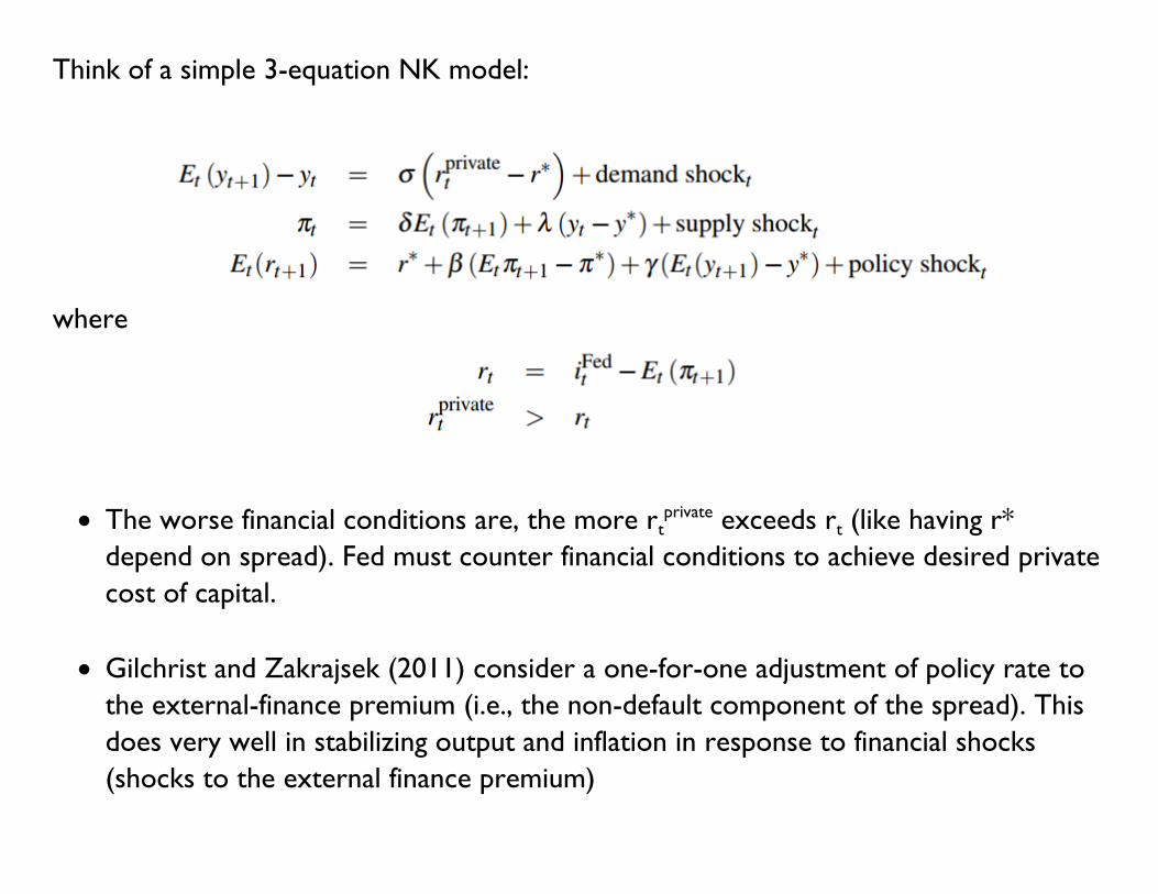
Think of a simple 3-equation NK model:
where
The worse financial conditions are, the more rtprivate exceeds rt (like having r*
depend on spread). Fed must counter financial conditions to achieve desired private
cost of capital.
Gilchrist and Zakrajsek (2011) consider a one-for-one adjustment of policy rate to
the external-finance premium (i.e., the non-default component of the spread). This
does very well in stabilizing output and inflation in response to financial shocks
(shocks to the external finance premium)
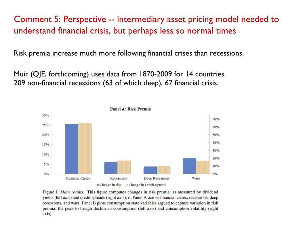
Comment 5: Perspective -- intermediary asset pricing model needed to
understand financial crisis, but perhaps less so normal times
Risk premia increase much more following financial crises than recessions.
Muir (QJE, forthcoming) uses data from 1870-2009 for 14 countries.
209 non-financial recessions (63 of which deep), 67 financial crisis.
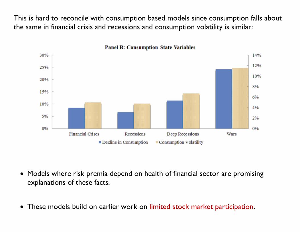
This is hard to reconcile with consumption based models since consumption falls about
the same in financial crisis and recessions and consumption volatility is similar:
Models where risk premia depend on health of financial sector are promising
explanations of these facts.
These models build on earlier work on limited stock market participation.
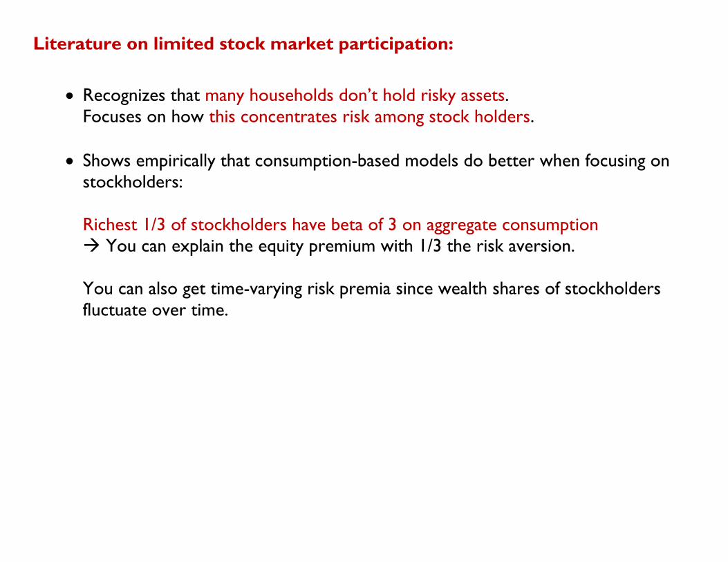
Literature on limited stock market participation:
Recognizes that many households don’t hold risky assets.
Focuses on how this concentrates risk among stock holders.
Shows empirically that consumption-based models do better when focusing on
stockholders:
Richest 1/3 of stockholders have beta of 3 on aggregate consumption
You can explain the equity premium with 1/3 the risk aversion.
You can also get time-varying risk premia since wealth shares of stockholders
fluctuate over time.

How do financial intermediaries fit into this?
The riskless asset is in zero net supply:
- In order for non-stockholders to do any saving in the riskless asset,
stockholders issue riskless assets to non-stockholders.
Implicitly, stockholders set up banks to issue riskless assets (deposits) to non-
stockholders. Banks then holds risky assets on behalf of stockholders. So
stockholders hold some risky asset directly and some indirectly via banks.
- Stockholder leverage via banks contributes to increase the risk premium on
risky assets (and on bank equity).
He and Krishnamurthy (2013)’s setup is the limiting case where stockholders hold
stocks only in intermediaries who then buy risky assets:
- Agency problems lead to net worth constraint on intermediary manager.
- When constraint binds, risk premia increase further, above the limited
participation value.
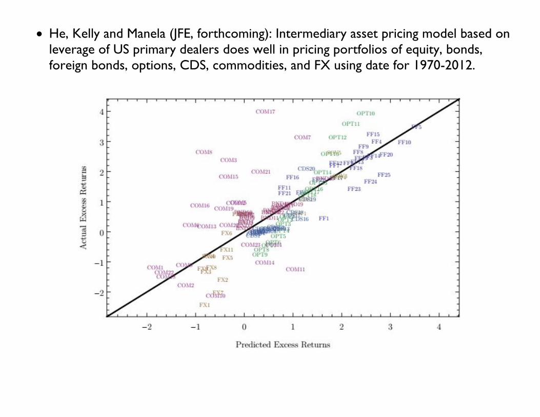
He, Kelly and Manela (JFE, forthcoming): Intermediary asset pricing model based on
leverage of US primary dealers does well in pricing portfolios of equity, bonds,
foreign bonds, options, CDS, commodities, and FX using date for 1970-2012.
Recommended