SHEAR WAVE MEASUREMENTS OF DEFORMATION
PROPERTIES OF SOIL
A thesis submitted to the University of London
for the degree of Doctor of Philosophy
in the faculty of Engineering
by
Colin Peter Abbiss
Imperial College
of Science and Technology
August 1983
Building Research Station
Department of the Environment
HFDAAA
ABSTRACT
The designer of a structure requires the deformation properties of the
ground in order to calculate the ground structure interaction. Shear
wave measurements in situ are described that enable these properties
to be calculated. Experiments using shear wave refraction and Rayleigh
wave measurements carried out on several different sites of clay and chalk
are described. Shear moduli as a function of depth are deduced from shear
wave velocities. A new method using the seismic noise on the surface of
the ground has also been developed and is shown to be another method of
applying the use of shear waves.
The properties of the ground are interpreted in terms of a generalised
theory of viscoelasticity. This enables the time dependence of moduli
to be related to damping at an equivalent strain. The mathematical
treatment is that of linear viscoelasticity, used as a first approximation
to the case of non linear viscoelasticity. Thus strain and time dependent
effects can be taken into account when comparing moduli measured by
geophysical methods with those obtained by direct methods.
The measurement of damping or quality factor in situ is therefore
important in order to calculate the deformation properties required for
many practical applications. Various methods of measurement in situ have
been investigated and are compared with published laboratory values.
Moduli measured by all three geophysical methods are compared with direct
measurements made by large plate tests, pressuremeter and back analysis
(ii)
using finite elements. When the appropriate corrections are made for
strain and time dependence good agreement is obtained.
Settlements are also calculated from the geophysical measurements for
loaded rectangular pads on boulder clay, a large tank on chalk and a
large silo also on chalk. These compared well with the observed
settlements.
(iii)

ACKNOWLEDGMENTS
The help of other members of the Geotechnics Division at the Building
Research Establishment is gratefully acknowledged. Many people have
cooperated in these experiments, especially Andrew Charles and
Ken Watts who carried out the plate loading test in the North Field,
also Charles Bryden Smith who installed the deep datum. Andy Gallagher
was responsible for the cyclic loading measurements on piles and he and
Don Burford assisted in the deployment of the geophone array on the sea-
floor at Christchurch Bay. John Cheney has consistently helped with
electronics, the setting up of the laboratory and precise surveying.
Bob Cooke and Gerwyn Price made their experimental facility available at
Brent and Paul Tedd arranged for the use of the swimming pool in
Bricket Wood.
Direct assistance was provided by Philip Elms who helped in the rebuilding
of the gauges under the silos and the development of the new AM version of
the seismic noise experiment. Kevin Ashby helped in the building of the
earlier electronics, made the marine measurements and also helped check
the mathematics of viscoelasticity. Eran Winkler helped write several of
the programs. Rosmarie Gates assisted with the feasibility studies and
also helped build electronic filters. John Austin participated in the
seismic shear wave experiments on clays. Mr Boden as Division Head
provided facilities and encouragement to continue with this work.
John Hudson has helped by critical reading of papers.
The drawing office and mechanical engineering workshop at BRE carried out
the detailed design and construction of the mechanical vibrator and have
(iv)

assisted in other ways. The wiring workshops wired the field version of
the seismic recorder and one of the magnet settlement gauges.
From Imperial College Andy Fourie assisted in the installation of gauges
at the silo site and read them at intervals during the loading season.
Especial thanks are due to Professor John Burland who has encouraged this
work from the start and whose judgement and guidance is highly valued.
(v)
CONTENTS Page No.
ABSTRACT ii
ACKNOWLEDGMENTS iv
CONTENTS vi
LIST OF FIGURES x
LIST OF TABLES xiii
NOTATION xiv
CHAPTER 1 INTRODUCTION, CURRENT METHODS OF MEASURING 1
THE PROPERTIES OF STIFF MATERIALS
1.1 Ground parameters and design 1
1.2 Review of present methods of measuring ground properties 4
1.2.1 Sampling 4
1.2.2 The oedometer 5
1.2.3 The triaxial test 5
1.2.4 The plate test 6
1.2.5 The pressuremeter 7
1.3 Application to calculation of settlement 8
1.3.1 Elastic treatment 8
1.3.2 Finite elements 9
1.3.3 Analytical 11
1.4 Time and strain dependent properties 13
1.5 Geophysical methods of measuring ground properties 14
1.5.1 Shear wave refraction 15
1.5.2 Surface waves 17
1.6 The use of precise surveying to verify measurements 18
(vi)

CHAPTER 2 SHEAR WAVE MEASUREMENTS
2.1 Seismic refraction
2.1.1 Site on Boulder clay, North Field at BRS
2.1.2 Site on London clay, Brent
2.1.3 Site on Gault clay, Madingley
2.1.4 Site on chalk of silos
2.1.5 Site on chalk of CERN test tank, Mundford
2.2 Associated p-wave surveys
2.3 Corrections and limits to refraction measurements
2.3.1 Pulse broadening
2.3.2 Signal to noise ratio
2.3.3 Hidden layer
2.4 Surface waves
2.4.1 Rayleigh waves
2.4.2 North Field BRS
2.4.3 Brent
2.4.4 The calculation of depth
2.4.5 Transverse surface waves
2.4.6 Deep measurements
CHAPTER 3 SEISMIC NOISE METHOD
3.1 Advantages of using seismic noise
3.1.1 Correlation techniques
3.2 The method
3.2.1 Filtering
3.2.2 The geophone array and calculations of velocity
3.2.3 The recording system
Page No.
23
23
32
35
39
39
41
43
49
49
52
53
53
53
58
60
63
66
66
70
70
72
73
73
75
79
(vii)

Page No.
3.2.4 The analysis system 81
3.2.5 Interpretation 82
3.3 Measurements 86
3.3.1 Site on Boulder clay, swimming pool at Bricket Wood 86
3.3.2 Site on London clay, Brent 86
3.3.3 Marine site on Barton clay at Christchurch Bay 87
3.3.4 Site on chalk of silos 89
3.3.5 Site on chalk of CERN test tank, Mundford 91
CHAPTER 4 TIME AND STRAIN DEPENDENCE OF MODULUS 93
4.1 Time dependence 93
4.1.1 Theory 93
4.1.2 Damping 96
4.1.3 Mathematical models 99
4.1.4 The generalised viscoelastic solid 102
4.2 Strain dependence 103
4.2.1 Effect of non linearity 103
4.2.2 Functional form of strain dependence of damping 107
4.2.3 Calculation of radius of curvature 111
CHAPTER 5 SOME EXAMPLES OF THE MEASUREMENT OF 113
IN SITU DAMPING
5.1 In situ methods 113
5.1.1 Hammer damping 113
5.1.2 Plate resonance 117
5.1.3 Pulse broadening 119
5.1.4 Attenuation coefficient 120
(viii)
Page No.
5.1.5 Comparison with hysteresis loops from plate tests 121
5.2 Damping factor (1/Q) as a function of strain 124
5.3 Measurement of Q by autocorrelation of seismic noise 124
CHAPTER 6 COMPUTED MODULI COMPARED WITH OTHER 131
IN SITU MEASUREMENTS
6.1 Dynamic moduli 131
6.1.1 Corrections to dynamic moduli 131
6.2 Comparison with other measurements 137
6.2.1 Comparison with plate tests at Brent 137
6.2.2 Comparison with pressuremeter at Madingley 140 6.2.3 Comparison with in situ values at Mundford 144
6.3 Accuracy 146
CHAPTER 7 CALCULATION OF SETTLEMENT 149
7.1 Methods of calculation 149
7.2 1 m square pads in North Field BRS 150
7.2.1 Three dimensional consolidation 156
7.3 Large silos founded on chalk 159
7.4 Test tank on chalk at Mundford 162
CHAPTER 8 CONCLUSIONS 165
REFERENCES 173
APPENDICES 1 MATHEMATICS OF VISCOELASTICITY 179
2 CIRCUITS 18?
3 PROGRAMS 188
(ix)
LIST OF FIGURES Page No.
2.A Plot of 2G/pV2p against V 24
2.1A Shear wave generator 25
2.IB Survey arrangement 26
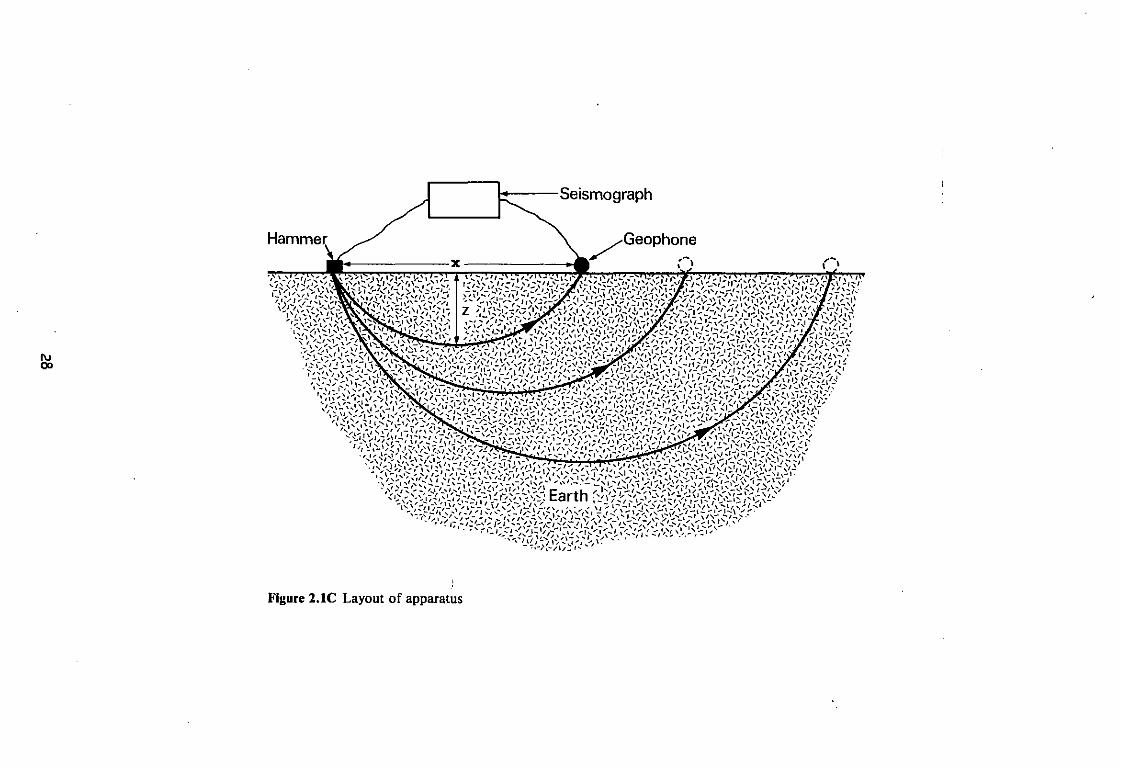
2.1C Layout of experimental apparatus 28
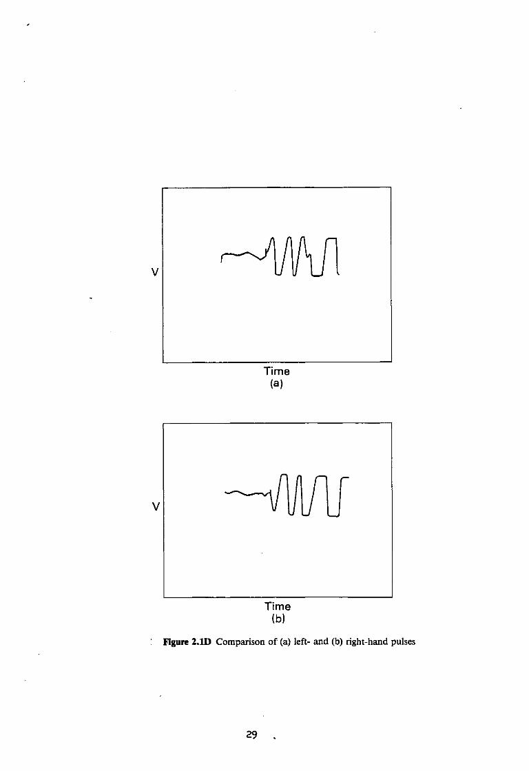
2.ID Comparison of (a) left- and (b) right- going pulses 29
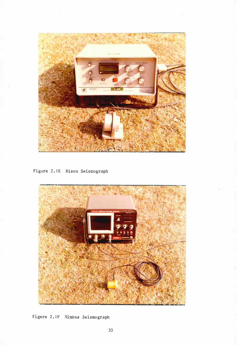
2.IE Bison Seismograph 30
2.IF Nimbus Seismograph 30
2.1G S-wave survey 31
2.1H S-wave refraction North Field (BRS) 33
2.11 S-wave pulse velocity against depth - North Field (BRS) 36
2.1J S-wave pulse velocity against depth - Brent 38
2.IK S-wave pulse velocity against depth - Madingley, Cambridge 40
2.1L S-wave refraction and seismic noise velocities, 42
Grade IV chalk
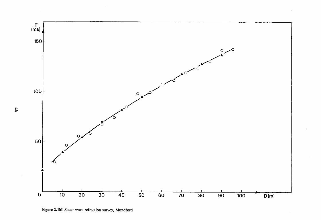
2.1M Shear wave refraction survey, Mundford 44
2.IN S-wave refraction and seismic noise velocities, Mundford 45
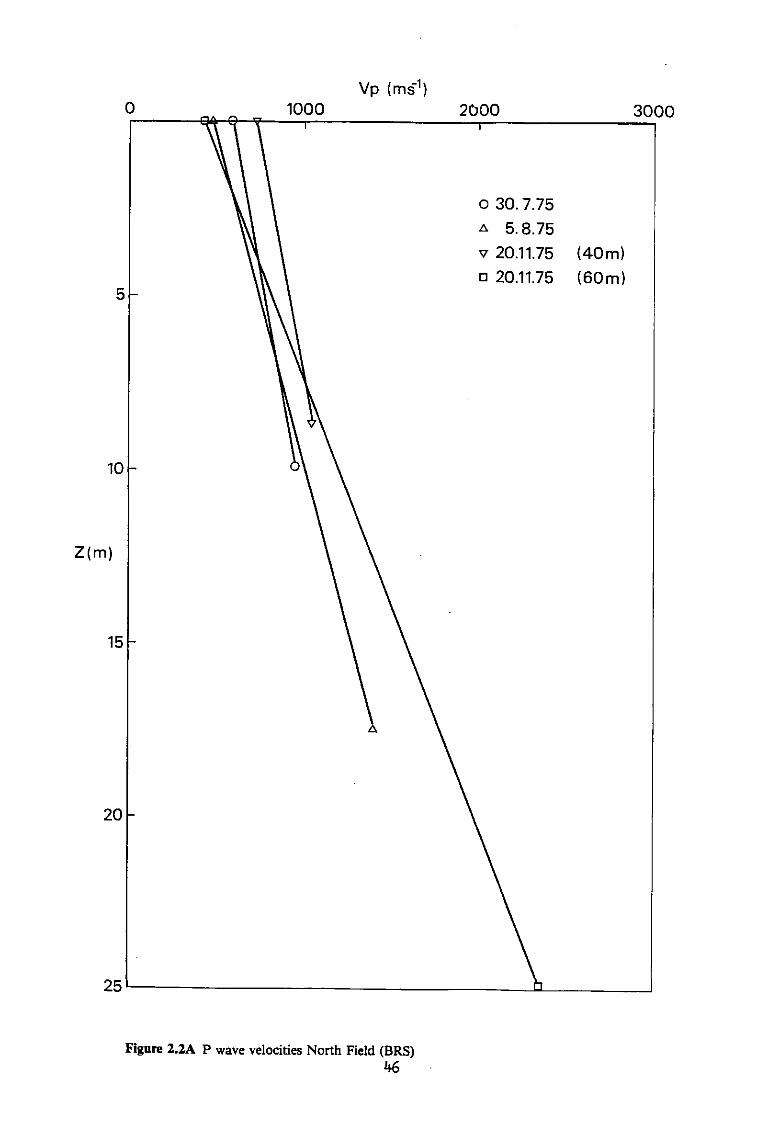
2.2A P wave velocities North Field (BRS) 46
2.2B P wave velocities Brent and Madingley 47
2.3A Pulse broadening 50
2.4A Rayleigh wave experiment 55
2.4B Electromagnetic vibrator and geophones 56
2.4C V„/V as a function of V /V 57 R s s p 2.4D Mechanical vibrator and geophones 59
2.4E Rotating weights of vibrator 59
2.4F Rayleigh waves and S 0 refraction (pulse) North Field (BRS) 61 2.4G V at Brent 62 s
(cdxxiv)

Page No.
2.4H Rayleigh wave velocity, wet mix macadam 65
2.41 Seismic velocities derived from a cross correlogram 69
3.1A Correlation curve on screen of correlator 74
3.2A Correlation curve 76
3.2B Wave velocity vector 76
3.2C Recording system showing one geophone in holder 80
3.2D Equipment for analysis of signals 80
3.2E Seismic noise velocities V against depth z for 83
swimming pool
3.2F Seismic noise velocities V against depth z for Brent 84
3.2G Seismic noise velocities V against depth z for 85
Christchurch Bay
3.3A Geophone in holder suspended from corner of frame 88
3.3B Marine recording system 88
3.3C Shear wave velocities from refraction and seismic 92
noise, Mundford
4.1A Viscoelastic response to applied stress 95
4.IB Complex compliance 95
4.1C Hysteresis loop 95
4.ID Damped vibration 98
4.IE Broadening of resonance peak 98
4.IF The standard viscoelastic solid 100
4.2A Damping ratios for saturated clays, from Bolton Seed 104
and Idriss
4.2B Modulus as a function of time and strain 106
4.2C Damping as a function of strain for saturated clays 108
4.2D Theoretical curves of damping against strain 109
(xi)
Page No. dD D2 2e 1 dine D m er (e-1)
4.2F Relation between modulus, Q and radius of curvature 112
5.1A Hammer damping, arrangement 115
5.IB Hammer damping 116
5.1C Plate resonance, Brent 118 5.ID Accelerations measured at Westminster 122 5.IE Plate tests at Brent Cross 123
5.2A Hysteresis loops 125
5.3A Autocorrelation for chalk at Mundford 127 5.3B Autocorrelation for boulder clay, North Field BRS 128 5.3C Autocorrelation for chalk, site of silos 129
6.1A Shear moduli G, Brent (low strain) 134
6.IB Shear moduli G, North Field (BRS) 135
6.1C Dynamic moduli from seismic noise 136
6.2A Comparison with plate tests at Brent 138
6.2B Comparison with Windle and Wroth, Madingley 141
6.2C Comparison with pressure meter measurements, Cambridge 142
6.2D Comparison with plate tests and finite elements, Mundford 147
7.2A 1 m square pad, 1.0 m depth, North Field 151
7.2B 1 m square pad, 0.3 m depth, North Field 151
7.2C North Field pad settlement, 1.0 m depth 153
7.2D North Field pad settlement, 0.3 m depth 154
7.2E G as a function of e for 1 hour 155
7.2F North Field pad settlement, 1.0 m depth compared with 157 3D consolidation
7.2G North Field pad settlement, 0.3 m depth, compared with 158 3D consolidation
7.3A Large silos founded on chalk 160
7.4A Test tank, on chalk at Mundford 163
(xii)

LIST OF TABLES Page No.
CHAPTER 2
2.1A s-wave, North Field (pulse) 34
2.IB Mean s-wave velocities, North Field (pulse) 34
2.1C s-wave, Brent (pulse) 37
2.ID Mean s-wave velocities, Brent (pulse) 37
2.IE s-wave, velocities, Madingley (pulse) 37
2.2A p-wave pulse velocities 48
2.2B Poisson's ratio 48
2.3A Ratios of pulse to continuous wave velocities 52
CHAPTER 3
3.2A Possible combinations of times 77
CHAPTER 5
5.3A Q from autocorrelation 130
CHAPTER 6
6.1A Dynamic G and E as a function of depth 132
(continuous wave)
6.IB Dynamic G^ and E from seismic refraction (pulse) 133
6.2A Comparison with plate tests at Brent 139
6.2B Comparison with Windle and Wroth 139
6.2C Cambridge, Madingley 143
6.2D Poisson's ratio, Mundford 145
6.2E Moduli, relative to depth below tank, Mundford 145
CHAPTER 7
7.2A G as a function of strain 159
7.2B Settlement from consolidation 159
(xiii)

NOTATION
A amplitude of vibration
a acceleration
B breadth
b radius of disc
c velocity of continuous wave, correlation function
c u undrained shear strength
D damping = 1 -t- , diameter
D^ maximum damping
d depth to a rigid base, distance
E Young's modulus, energy stored in cycle
E^ undrained Young's modulus
AE energy lost per cycle
e base of natural logarithms
f frequency
G shear modulus
G(0) shear modulus at surface
H layer thickness
J compliance A
J complex compliance
relaxed compliance
J u unrelaxed compliance
Jl real component of compliance
J2 imaginary component of compliance
j /-I
L length, length of triangle side M modulus £ M complex modulus
(xiv)

in coefficient of increase of G with depth
N power of e
n frequency
P maximum pressure O
Q mechanical quality factor, electrical quality factor
q loading pressure
r plate radius
T time, sample time
Ti delay time
Tp period of signal
t time, time constant
U impulse height
u height of pulse envelope
V wave velocity
V^jVp compression wave velocity
V velocity of pulse
Vg shear wave velocity
V R Rayleigh wave velocity
Vj a voltage varying with time
V2 another voltage varying with time
v voltage
W power radiated
w settlement
X retardation spectrum, numerical distance
x distance
y ln w
Z depth
z depth
(xv)
a attenuation coefficient
5 logarithmic decrement
e strain £ constant strain O
e^ representative strain
£]_ in phase strain component
£2 strain component 90° out of phase
0 1/Q, cot"1 G
X wavelength
v Poisson's ratio
p mass density a applied stress
02 principal stresses in x, y, z directions
T time constant
AT period of impulse
$ generating function
<J> an angle, phase angle, creep function w angular frequency
o>o transition frequency
(xvi)
CHAPTER 1
INTRODUCTION, CURRENT METHODS OF MEASURING THE
PROPERTIES OF STIFF MATERIALS TAn act of observation is ... necessarily accompanied by some disturbance
of the object observed' P A M Dirac
1.1 Ground parameters and design
Design considerations for the foundations of a structure require that the
designer has a clear idea of the expected performance of the system before
it is constructed. This involves a knowledge of how similar systems have
behaved previously, perhaps in similar circumstances, and also an analysis
of the system that is thought to correspond fairly closely to the way it
will behave in practice.
Thus Ideally the performance required of the system should be specified by
a set of parameters with upper and lower limits. The structure is
expected to behave in such a way that the parameters are always within
these limits. They will be set by the requirements of the owner and users
of the structure and the purposes to which it will be put. They will of
course include limits on cost.
The limiting parameters which most concern foundation engineers are
usually in the form of maximum movements, vertical, horizontal or
differential. Implied in these is the requirement that the foundation
must not fail, in other words that no movement should increase
progressively.
HFDAAB 1

The calculation of movements of a structure resting on the ground may
involve a thorough analysis of the ground structure interaction. Usually
computer analysis can tackle these problems with the parameters of the
structure being fairly well defined. The problem arises with the
properties of the ground with which the structure will interact. These
properties are characteristic of the particular site in question and may
vary with depth, with orientation, time, strain, moisture content and
other variables. The designer really requires these properties for the
conditions under which the ground will interact with the structure when in
use.
If these ground properties could be measured precisely for the conditions
under which the system will perform then the designer can calculate more
accurately the expected values of the design parameters with their upper
and lower limits. Of course no calculation of this kind is absolute and
certain probabilities of performance will be likely. The acceptable level
of probability will depend upon the type of structure.
Thus the ideal and maybe practical goal is that there should be what
Lambe (1973) called a 'class A' prediction made of deformation and
movement before the structure is commenced.
Stiff clays and weak rocks are particularly difficult to sample and test
by standard methods and give stiffnesses which are five to ten times too
low. However they have been shown to behave elastically at low strains.
It is for these materials that measurements by geophysical methods may
offer a better accuracy.
2

For these reasons methods of measuring the properties of stiff ground by
geophysical techniques have been investigated. These are carried out at
relatively small strains, below 100 y strain. In this way the actual fin situ', undisturbed, ground parameters may be made available to the
designer, so that he may carry out the 'class A' prediction, which in the
majority of cases, requires low strain information.
Current analytical techniques provide a means of accurately predicting
movements in the ground, either around excavations or beneath foundations.
The information required is the appropriate values of the modulus and
strength of the ground.
The problem is that there often exists a considerable inaccuracy in the
ground parameters. For example values for chalk obtained by correlation
with STP counts (Wakeling, 1974) may require multiplying by a factor of
10 or even 50. In fact bridges built on chalk for the Newmarket bypass
are not piled and perform quite satisfactorily (Burland, 1983).
Similar underestimates have occurred in London clay. At the House of
Commons underground car park vertical settlements and horizontal wall
movements were calculated satisfactorily on the basis of values of Young's
moduli that were up to nearly six times the value from oedometer tests
(Burland and Hancock, 1977).
The same kind of difference has been observed between triaxial tests on
98 mm diameter samples and 865 mm plate tests on the London clay. At
Hendon the first loading of plate tests gave values up to nearly four
times the mean from the triaxial tests. Reloading values were up to
3
three times larger. At Chelsea the plate tests gave twice the mean of the
triaxial tests.
1.2 Review of present methods of measuring ground properties
1.2.1 Sampling
Whatever sampling method is used, whether the sample is removed in a
thin walled tube, or a block of clay is cut out with a chain saw, the
sample is removed from its in situ conditions of stress. If the sample
is taken from any depth this stress will be considerable, of the order of
200 kNm""2 for 10 m depth. Although this overburden pressure may be
simulated in the laboratory the fact remains that the sample has been
taken through a destressing cycle and this stress path may well modify
Its behaviour under further testing. In other words many of these
materials have a 'memory' and their present response to applied stress is
a function of their past history. This would seem to account for the fact
that often the moduli measured in the laboratory from such samples is many
times less than the values from back analysis of observed strains or large
scale in situ testing.
Another problem that arises with taking a small laboratory sample is that
if it contains one or two large particles these may have a
disproportionate effect on the measured result. If the sample is a
fissured clay then the local fissure pattern may have a predominate effect
particularly on strength. A failed specimen often is seen to have failed
along a particular fissure. If the ground is thought of as having a
statistically varying set of properties about mean values then the problem
of taking small samples is evident. Ideally the size of the sample should
4
be large in comparison with these variations and with the scale of the
structure with which it will interact.
1.2.2 The oedometer
In the oedometer a sample is compressed between platens at either end of
a cylindrical holder. The sample is subjected to uniaxial compression
and ex vertical strain is measured due to the vertical stress ax while
£2 and £3 are kept equal and close to zero by the confining walls of the
holder. One of the problems with this system is the effects of bedding
errors at the ends of the samples which lead to overestimated values of
compressibility on first loading. Compressibilities of stiff ground
measured by oedometer tend to be several times larger than those
estimated from back analysis of settlements. In addition the confining
pressure will depend on the behaviour of the sample and the level of a\.
1.2.3 The triaxial test
In the triaxial test a cylindrical sample is subjected to a vertical
stress ax along its longitudinal axis while the horizontal stresses
<J2 and 03 are kept constant by a surrounding pressure chamber. The
difference between o\ and 03 is termed the deviator stress and written
as (ax -03). By varying deviator stress and confining pressure a
considerable range of stress paths can be simulated (Bishop and Henkel,
1957).
Large versions of the triaxial test apparatus have been built to cope with
samples with large particle size (Charles and Watts, 1980). This has
helped in the correlation with analysis of the overall behaviour of rock-
fill dams for example. Modifications to the standard equipment have
5

allowed long term tests to be run for periods of days. The test has been
carried out with cyclic loading, the sinusoidally varying stress being
applied by means of hydraulic rams.
Most of the theory of critical state soil mechanics has been built up
around observations in the triaxial test (Atkinson and Bransby, 1978).
1.2.4 The plate test
Many of the problems of sampling and size are overcome by large scale
In situ plate tests. A programme of such tests has been carried out at
The Building Research Station for over a decade. Work on high stiffness
chalk showed that values obtained from the plate tests correlated with
the moduli from the back analysis of the strains under a large water
filled tank (Burland and Lord, 1969). The plate diameter was 864 mm, in
effect testing a fairly large sample. Further work was carried out on
London clay (Marsland, 1971a, 1971b) with high moduli for the over-
consolidated clay resulting. These moduli showed a closer relation to
observed settlements and movements (St John, 1975, Burland and Hancock,
1977).
The problem remaining with the plate test is that there is stress relief
at the base of the borehole and a range of strains experienced under the
plate (Marsland and Eason, 1973). The conclusion from this work seems to
be that local low strain moduli may be twice the deduced overall value.
In addition the material under test has been subjected to an unloading
cycle when the borehole was made prior to the loading of the plate. The
moduli measured are a combination of vertical modulus E and horizontal v
modulus E, and correspond to fairly high strains. The material may be
6
taken to failure and moduli quoted are often secant moduli for half
ultimate strain. Average strains may be 0.2% and times of 0.6 mins.
With cyclic loading of the plates hysteresis loops can be observed
(Marsland and Eason, 1973, Gallagher, 1980).
The great advantage of this method is that it is in situ and with care
the disturbance of the sample can be reduced to a minimum. However, the
cost of such testing is very high and it is difficult to carry out under
water. Moreover the technique is of dubious value in soft soils.
1.2.5 The pressuremeter
Another method which shares this in situ capability is the self boring
pressuremeter. In the form used by Windle (1976) it produced little
disturbance, verified by x-ray photographs of lead shot buried in the
clay. Moduli are obtained by inflating a cuff which expands into the
material causing radial strain that is measured by strain gauges. The
moduli measured are strictly horizontal properties G^ and E^.
A push in version without the boring head was developed by the Building
Research Station. Called the PIP (push in pressuremeter) it was developed
for deployment on the sea floor by remote control (Henderson, Smith and
St John, 1979). It was tested at Madingley, Cambridge and Brent, London.
A fairly wide range of strains can be observed and the material taken to
failure. Average strains may be 0.75% with 2 mins taken for a reading.
The amount of equipment required is somewhat less than that needed for the
plate tests. In theory the material is not destressed by the system. In
fact the pressure may be raised locally by the positioning of the
7

pressuremeter. It would be much more difficult to apply in the case of
weak rocks.
1.3 Application to calculation of settlement
1.3.1 Elastic treatment
The classical theory of elasticity allows the calculation of the
settlement due to a loaded flexible disc on the surface of an elastic half
space (Boussinesq, 1885). The more familiar form is the settlement w of a
rigid punch acting on the edge of an elastic half space. In this case w
Is related to the pressure q acting over the face of the punch, the
Young's Modulus E, Poisson's Ratio v and the punch diameter D by
» = i.i
This is the formula used in the calculation of E from the plate tests,
where is the depth correction factor.
Thus the input required for the calculation is the pressure, the geometry
and the equivalent elastic properties of the ground beneath the
foundation. All calculations of settlement require this information
although the treatments may differ (Burland, Broms and De Mello, 1977).
Implicit in the elastic theory is the Boltzmann superposition theorem,
that is that the strains due to all the loads are a sum of the strains due
to the individual loads acting independently. The classical treatment
allows the loads to be idealised as a distribution of point loads, which
simplifies the analysis.
8

An elastic model shows no time dependent effects. The strains are
produced at the instant that the stresses are applied, there is no creep
and the strains are reversible. Clearly an elastic treatment is at best
a first approximation to the conditions that are usually found in the
ground.
The classical elasticity theory can be used to find stress distributions
beneath a loaded pad. These are well known and examples may be found in
Lamb and Whitman (1969). They are used to cope with the situation where
the ground may be considered to be made up of a series of horizontal
layers each with a different stiffness. The stress distribution curves
are used to find the average stress in each layer and the appropriate
compression of each layer calculated from its modulus or compressibility
m^. The total settlement is then the sum of the compression of all the
layers.
Time dependent effects may be taken into account by assigning different
moduli for different time periods. Thus the immediate settlement
corresponding to a time of 24 hours is calculated from a modulus that is
somewhat higher than that needed for several months. The difference is
often explained in a clay for example by the drainage of pore water.
1.3.2 Finite elements
Even with the elastic model it is difficult to cope with a range of
geometries and varying properties. The method of finite elements has been
of great use in these situations. Although generally confined to
calculations carried out in one plane, the situation of plane strain, it
has been able to cope with strains underneath foundations, piled
9
foundations, movements around excavations and strains in earth and
rockfill dams.
A mesh of finite elements intersecting at nodes simulates the ground.
These elements are usually elastic and can vary in stiffness from one to
another. The calculation is carried out by computer. In theory the
limits on accuracy are the fineness of the mesh and the number of nodes.
In practice this means that the limits are set by the capacity of the
memory and the speed of the computer. Three dimensional calculations with
a large increase in the number of nodes are not often carried out,
although the corner of an excavation has been successfully analysed (St
John, 1975). The program used had difficulty dealing with variation of
modulus with depth.
A recent development has been the program that generates its own pattern
of nodes most appropriate for the problem in hand.
Finite elements were used to back analyse the strains underneath a tank
on the chalk at Mundford (Burland, Sills and Gibson, 1973). The analysis
showed that the chalk had properties similar to a Gibson soil, increasing
in stiffness with depth, that the values were of the order of thousands of
MNm""2 and the plot of stiffness against depth passed through the values
found from the plate tests.
The case of a raft of varying stiffness resting on a soil that has a
modulus increasing with depth has been studied by finite element
computations at the Building Research Station and is described in
HFDAAC 10
Burland and Wroth (1974). Settlements at the edge and centre were
compared with those of a block of flats on a raft on London clay. A
review of structure/soil interaction is given in a State of the Art
Report published by the Institution of Structural Engineers in 1977.
Currently finite elements are being used at Imperial College to analyse
the strains under four silos each carrying up to twelve thousand tonnes
founded on grade four to five chalk and their interaction with a new
twenty five thousand tonne silo set to one side in relation to the line of
the other four. Strains beneath the silos are being measured by precise
magnet extensometers (Smith and Burland, 1976).
Most finite element calculations assume elastic behaviour. The method is
being developed to deal with non linear plastic materials and time
dependent materials.
1.3.3 Analytical
The strains under the tank at Mundford were calculated analytically for
a material whose stiffness increased linearly with depth by Burland,
Sills and Gibson, (1973). Agreement with observed strains on the whole
was good except for the surface where the calculated strains went off to
a high value, due in effect to the modulus approaching zero at the
surface.
Awojobi and Gibson (1973) tackled the problem of the Gibson soil and
arrived at expressions for the settlement in terms of the pressure, the
stiffness of the surface and the increase of stiffness with depth. These
relations have been used at Cambridge University to calculate the
11

magnitude of seismic noise at low frequencies due to fluctuations of
barometric pressure. By using the moduli found from seismic wave
measurements the amplitudes of the noise can be found correctly.
The problem has also been treated by Brown and Gibson (1972) where surface
profiles have been calculated for a flexible disc producing a uniform
loading resting on a deep elastic stratum with shear modulus G increasing
linearly with dept G(z) =G(o) + mz. The solutions involve confluent
hypergeometric functions which were calculated numerically. They show the
surface profiles at different distances from the centre for Poisson's
Ratio of 0, 0.3 and 0.5. They also give the central displacement as a
function of G(o)/mb where b is the radius of the disc for the same values
of Poisson's ratio.
In a later paper Brown and Gibson (1979) examine the case of a rectangular
pad producing uniform loading and resting on a layer with modulus
increasing with depth to a maximum finite depth. They give a set of
curves of corner settlement against length to breadth ratio for different
ratios of pad size to layer depth and for different degrees of
inhomogeneity and Poisson's ratio.
Both the finite element and the analytical calculations emphasise the
importance of measuring the variation of modulus with depth with
particular emphasis on properties near the surface or just below the
foundation. The appropriate value of Poisson's ratio is also seen to be
important.
12

1.4 Time and strain dependent properties
The settlement is in fact often time dependent and on a material such as
London clay, this is recognised by the calculation of immediate and long
term settlements. By immediate, a period of twentyfour hours is usually
understood. The long term settlement may refer to periods of years.
This time dependence is allowed for by assigning two moduli to the clay,
the first E^ the undrained Young's modulus is used to calculate the
immediate settlement and E' the drained or effective stress modulus is
used for the long term calculation. These two moduli are related and one
may be found from the other by taking the behaviour of the pore water into
account.
This illustrates a more general point that these moduli are indeed time
dependent and strictly should be written as G(t) or E(t). This time
dependence extends down to the time scale of geophysical measurements of
the order of tens of milliseconds. The class of materials that show these
time dependent effects are the viscoelastic solids where Hookes Law is
modified to the form
e - | [l + <f>(t)] 1.2
where e is the strain, a is the stress, M the modulus and $(t) a creep
term.
In addition the moduli will be strain dependent and should be written as
G(e,t). This is seen very clearly in the curves given by Bolton Seed
and Idriss (1970) and in the stress strain curves of the plate tests
(Marsland, 1971).
13

Hence a settlement calculation may be iterative, an approximate value of
the strain being found in order to use the modulus appropriate for that
level in the next step of the iteration and so on. Finite element
programs can also deal with non linear properties. Fortunately many
settlements under lightly loaded foundations correspond to small values
of strain where the modulus is not varying greatly with strain. This
also is not too far from the levels of strain under which the geophysical
measurements of wave velocity are made, the modulus being calculated from
the wave velocity.
1.5 Geophysical methods of measuring ground properties
For an ideal elastic homogeneous material the modulus is directly
proportional to the square of the wave velocity.
E = nV 2 (l~2v)(l+v) 3 E pvP — U ^ D
where E is the Young's modulus, p the mass density, V^ the
compression wave velocity and v the Poisson's ratio - Ambraseys and
Hendron (1968),
and G = pV 2 1.4 s where Vg is the shear wave velocity.
The traditional measurement has been the compression wave velocity and
papers report this for London clay (Ward, Marsland and Samuels, 1965) for
Gault clay (Samuels, 1975) and chalk (Grainger, McCann and Gallois, 1973).
Correlation with modulus was reported by Brown and Robertshaw (1965) for
a range of materials, see also Davis and Taylor Smith, 1980.
14

The problem with calculating the modulus from V^ is the value of Poisson's
ratio to be used in the term (l-2v) in equation 1.3. If v is close to 0.5
then the modulus becomes extremely dependent upon this term, and low
values of modulus may be hidden by high compression wave velocities.
In some cases where the Poisson's ratio is believed to be low ** 0.24
the formula can be used satisfactorily (Abbiss, 1979). However this does
lead to a difference between dynamic and static moduli that must be
explained by recourse to viscoelasticity theory.
The two main experimental techniques used traditionally are the
measurement of compression wave pulses through cylindrical specimens and p
wave seismic refraction from the surface of the ground. Cross hole
shooting is also sometimes carried out.
Seismic refraction is used on the whole to determine the depth of
refracting layers rather than to make quantitative measurements of moduli.
1.5.1 Shear wave refraction
Shear waves on the other hand have a direct relation to shear modulus via
equation 1.4 that does not depend on Poisson's ratio. A high modulus will
be indicated by a high shear wave velocity and a low modulus by a low
velocity (Davis, 1980).
The various kinds of shear waves that can be used in a civil engineering
context are discussed by Mooney (1974). He points out that it is much
better to make measurements in situ rather than on samples in the
laboratory and says that the case of S^ waves, those that are horizontally
15

polarised, is particularly straightforward. This is the situation that
is encountered in the shear wave refraction experiment with a horizontal
impact as the source and horizontal s-wave geophones as detector. He also
shows that the case of Sy waves, those polarised in the vertical plane, is
much more difficult to cope with and interpret correctly. Also discussed
are various types of source of s waves, and he states that a clear
reversal of wave form can be obtained by reversing the direction of the
horizontal impact at right angles to the direction of the survey line.
The problem with the interpretation of all the hammer impact refraction
experiments in the context of a soil is that it is a pulse that is being
timed. If the material exhibits viscoelastic properties then the pulse
velocities will differ from the velocities of continuous waves that
correspond to the elastic case. The propagation of a pulse in a visco-
elastic material is dealt with by Ricker, who shows that generally pulse
broadening occurs and that this speeds up the leading edge of the pulse.
There are ways of correcting for this effect using formulae given by
White (1965) but this has not been carried out previously.
A second paper by Mooney (1976) deals with the behaviour of pulses
travelling from a surface impact. Theoretical waveforms were only
compared with experimental results in the context of pulses propagating
over short distances in a granite block where conditions were close to
ideal elasticity, and viscoelastic effects would not be so noticeable.
He also calculates the effect of variations of Poisson's ratio upon pulse
length and shows an increase of pulse length with Poisson's ratio for
longer distances.
16
1.5.2 Surface waves
Another group of experiments uses the properties of surface waves first
investigated by Lord Rayleigh (1900). In this case waves can be
generated continuously by a vibrator standing on the surface of the
ground. According to Miller and Pursey (1955) some 67.4% of the energy
will go into the form of surface waves of a particular type known as
Rayleigh waves. These have the particle motion in the form of a
retrograde ellipse in the vertical plane containing the direction of
propagation. The amplitude dies away exponentially with depth to close to
zero at a depth of one wavelength. By measuring the relative phase of
signals detected by geophones at a known separation the wavelength X may
be determined. With the frequency n measured the velocity V R can be
obtained from
VR => nX 1.5
Work using this method is reported by the Waterways Experiment Station
(WES), (Ballard and McLean, 1975; Cunny and Fry, 1973) who describe both
refraction experiments and surface wave measurements. They claim that
the surface wave test is reliable and that good correlation is found with
borehole information. By assigning the velocity measured to a depth of
half a wavelength X/2 variations of properties with depth can be measured.
Ballard and McLean report a case of a layer of low velocity beneath
higher velocities. The problem in making measurements at greater depth
is that a strong vibratory source working at low frequencies is required.
Maxwell and Fry (1967) report experiments of this kind that show clear
linear dependence of phase on distance with different slopes for different
frequencies and compute moduli down to a depth of approximately 33 m. In
these earlier experiments phase was measured by observing waveforms on
17

the screen of an oscilloscope. Good correlation was obtained with
conventional boring logs and moduli increased with depth.
R Jones (1958) at the Road Research Laboratory investigated the behaviour
of Rayleigh waves and another transverse surface wave known as the Love
wave. A geophone was placed at varying.distances from the electromagnetic
vibrator and the number of wavelengths plotted as a function of distance
from the vibrator for the Rayleigh waves. Dispersion curves of velocity
against frequency were deduced for these measurements and also for Love
waves. Both types of experiment were explained in terms of a layer of
brick earth of thickness H overlaying a gravel layer of higher velocity.
Theoretical dispersion curves were calculated on the basis of a
mathematical model. The values of Q obtained were quite close to the
observed depth. Rayleigh wave velocity also was compared with California
Bearing Ratio (CBR) values, which increased with velocity. Shear modulus
values obtained by equation 1.4 were compared with moduli found by
resonance methods on two sites and the agreement was within the range of
values from the resonance experiments.
In addition surface wave measurements had been made on roads (Heukelom and
Foster, 1962) where a clear distinction can be made between the different
layers, and transitions could be located by assigning the depth of
measurement to one half wavelength X/2. These shallower measurements were
made at higher frequencies.
1.6 The use of precise surveying to verify measurements
In a general paper discussing the measurement of ground strain in civil
engineering (Ward and Burland, 1973) it is pointed out that the strains
18

measured are often very small in the region of 10~6 or even 10~7. This is
accomplished by precise surveying over distances of tens or hundreds of
metres. For the precise measurement of settlements and lateral movements
around excavations the deformations sometimes must be measured to tenths
or hundredths of millimetres.
The cases cited include the measurement of strains under a large tank on
the Middle Chalk at Mundford where measurements were made by inductive
transducers attached to invar wires and precise water level gauges. The
former gave vertical displacements to 5 x 10~3 mm. Other examples
described were measurements under and around deep excavations in London
clay for the basements of tall buildings and also the underground car park
at the Houses of Parliament. Standard precise surveying methods were used
to relate the movements to regions outside the influence of the
deformations. The vertical movements were observed by precise levelling
and the lateral movements by theodolite measuring horizontal displacements
to within 1 mm.
Measurements on a rockfill dam at Scammonden are also described where the
movements within the dam were related to an external reference pillar by
means of the Mekometer, a precise electro optic distance measuring
instrument. This instrument has a resolution of tenths of a millimetre
at a range of hundreds of metres and an accuracy of ± 3 x 10"6
(Froome, 1971).
All the optical surveying techniques have a fundamental limit to their
accuracy set by the fluctuations or departures from uniformity of the
refractive index along the line of sight. This causes errors of about
19

3 x 10"6 for the Mekometer while combined with optical limitations in
theodolites an alignment of 1 second of arc is possible with a precise
instrument under good surveying conditions. This is equivalent to 1 mm
at a range of 200 m, 0.1 mm at 20 m. These accuracies mean that with
standard precise surveying techniques the deformations observed must be
due to fairly considerable stresses, as high as 100 kNm""2 in order for
the strains to be observed with reasonable accuracy. There is a case for
improvement in the accuracy of measurement of settlement so that lighter
loading can be used.
The standard precise levelling technique, with due attention to levelling
points and reference datum, (Cheney, 1973) can measure settlement of a
loaded pad or foundation to within ± 0.1 mm over quite long periods of
time. It is more difficult to make rapid measurements at the other end
of the time scale. However pad settlements will be described in a later
chapter that were made satisfactorily over the time range 102 to 105
seconds. The advantage of the method is that commercially available
precise levels and staves can be used and that the installation of the
datum is not too expensive or difficult. However the datum is important
as the levelling technique gives information only about relative vertical
movements. This method also has the advantage that it can be applied
directly to buildings and structures by installing points in walls or
foundations.
Another method of measuring the vertical strains in the ground under a
foundation is the BRE magnet extensometer (Burland, Moore and Smith,
1972). Circular magnets are located by means of spring holders and
grouting around a tube containing reed switches attached to a stainless
20
steel tape. Relative movements are indicated by the change of relative
closure positions of the reed switches. The tape is raised and lowered
through the magnetic fields by a micrometer head at the surface of the
ground. In this way movements of the top magnet just below the foundation
can be related to the position of the datum magnet some 30 m below.
Provided that this datum magnet is out of the region of influence of the
foundation this information will give absolute settlements of the
foundation. Measurements made under some large silos will be compared
with wave velocity data in a later chapter. This system is capable of
reading the position of each magnet to about 0.1 mm so that relative
movement of the foundation magnet can be read to 0.2 mm. Other magnets
distributed along the extensometer allow the mapping of the strain field
underneath the foundation where it intersects the field of the
extensometer.
Making measurements of strains at various depths has the advantage that
one should be able to relate them to the varying properties as a function
of depth. Otherwise if the measurement is confined to surface movements
then an average property, described perhaps in the form of a Gibson soil,
is all that can be deduced.
Perhaps the best system used was that under the tank at Mundford where
inductive transducers measured movements of the different levels
relative to a vertical invar wire. The accuracy was high, ± 5 x 10~3 mm,
and strains were measured at six different levels thus enabling the
calculation of the variation of the properties with depth, even though
the stiffnesses were high and the strains correspondingly small.
21

Other methods of measuring deflection and especially vertical settlement
would seem to be worthwhile investigating especially if they could be
used with lighter loads more easily transported to a site. A laser
interferometer has been tried with some success. Tiltmeters are another
possibility and even seismometers with feedback giving long time constants
might be used.
These measurements of strain constitute the true test of the validity of
the measurements of stiffness in the ground and of the calculations of
movement as a result of applied stress. When proved satisfactory in the
case of simple circular and rectangular pads they can then be applied to
more complicated cases.
22

CHAPTER 2
SHEAR WAVE MEASUREMENTS
The direct nature of the relationship between shear wave velocity and
shear modulus is shown clearly by equation 1.4 where G = pV 2. This does 5
not include Poisson's ratio and so shear wave velocity is a true indicator
of effective ground stiffness. This is not necessarily so for the
p-wave velocity where the modulus may depend to a large extent upon
Poisson's ratio v see figure 2A. pVp2(l-2v)
2(l+v) G - — E _ _ 1.6
If v is close to 0.5 the upper bracket will be near zero and a low modulus
will be associated with relatively high p wave velocity.
In this investigation measurement of shear wave velocity in the ground has
been carried out by broadly two methods. The first uses waves generated
mechanically and times their passage through the ground. The second, to
be dealt with in the next chapter, makes measurements on naturally
occurring seismic waves.
2.1 Seismic refraction
The seismic refraction experiment used horizontally polarised shear waves
generated by the impact of a horizontally moving hammer on an aluminium
channel section in contact with the ground surface and weighed down by the
wheels of a Land Rover or van, figure 2.1A. The waves produced were
horizontally polarised S^ waves. The direction of the pulse could be
reversed by the use of two swing hammers in opposite directions,
figure 2.IB. The pulses were detected by an s-wave geophone parallel to
HFDAAD 23
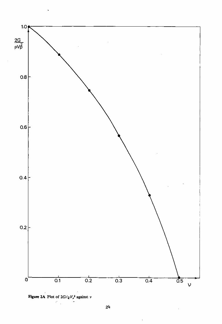
Figure 2A Plot of 2G/qVP2 against v 24

Figure 2.1A Shear wave generator
25

Figure 2.IB Survey arrangement
26

the channel section at a distance x from the source, figure 2.1C. The
comparison of left going and right going pulses is shown in figure 2.ID.
This enabled the positive identification of s waves arriving after the
p-wave pulses. The signals were stored and displayed by a Bison seismo-
graph in the first experiments and a Nimbus seismograph in the later
experiments. Both instruments, see figures 2.IE and 2.IF digitise the
signal and store it in a memory while displaying the wave form on a
cathode ray tube. This makes possible the enhancement of the signal,
repeated pulses being 'stacked' or added in the memory with the resultant
displayed on the screen. Enhancement helps to overcome the inherent
signal to noise problem due to the background noise. Up to five impacts
were used at the greatest distance.
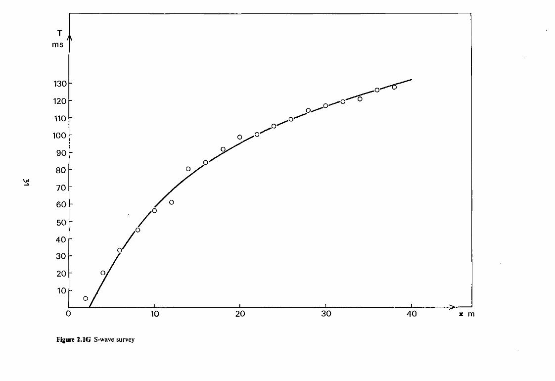
The arrival time T of the leading edge of the s wave pulse was plotted
against distance x and is shown in figure 2.1G, for the North Field site.
These time distance curves were fitted by the formula
This was carried out by a programmable calculator, the HP 67 see program
in Appendix 3, or by computer. The formula assumes that the seismic
velocity increases linearly with depth according to
where VQ is the velocity at the surface and Z is the depth.
A full derivation of this formula is given by Nettleton (1940). This was
a good first approximation to the behaviour of the velocity as a function
of depth. Another method in which the ground is assumed to consist of n
sinh-1 ^ 2V 1.7 o
V(z) = V + kZ 1.8
27
Seismograph
Hammer
'J</J V' 'l \
ro oo
I Figure 2.1C Layout of apparatus
Time (a)
Time (b)
Figure 2. ID Comparison of (a) left- and (b) right-hand pulses
29
: l : • . - ^
Figure 2.IE Bison Seismograph
V v I 'a • ifa-f % SJ*
Figure 2.IF Nimbus Seismograph
30
0 10
Figure 2.1G S-wave survey
30 40

layers as described by Morris and Abbiss (1979) is compared in figure 2.1H
where it also produces a linear variation of velocity with depth. The
difference is only 5% at 14 m depth. In addition a logarithmic function
was fitted to the time distance data and the n layer model applied to that
with similar results.
Another calculator program has been written which finds the depth Z
corresponding to the distance x and also enables one to find the maximum
depth Z for the maximum range x of the survey. The formula used is ui3x mflx
Finally as a check a program has been written which generates values
of sinh"1 using the formula sinh x = ln[x + / (x2 + 1)] to compare O
values of T found from the analytical formula with the original
experimental data ie to check that the fit is good visually.
It was decided to test this technique on three sites with stiff clay where
comparisons with other methods and settlements could be made. In addition
two sites with different qualities of chalk were investigated.
2.1.1 Site on Boulder clay, North Field at BRS
Shear wave refraction surveys were made at the Building Research Station
on the North Field site. The site consists of Boulder clay overlaying
chalk which, from boreholes at another site on the Station, was at about
19 m depth. The technique used was that described previously and the
results of four surveys are given in Table 2.1A. The fits were carried
out by calculator program. The standard errors were small, in two cases
32

V(ms~1)
Figure 2.1H S-wave refraction North Field (BRS)
33

TABLE 2.1A S-WAVE NORTH FIELD (PULSE)
Date AT millisecs k(s"J) V (ms"1) 0 a range
(m) Z (m; max
30.7.75 2 41.0 104.3 - 0,48 0 - 4 0 17.6
18.11.75 6 34.0 176 0,32 0 - 4 0 15.5
4.8.76 3 56.0 90.9 - 0.4 0 - 3 0 13.5
26.1.77 2 56.0 64.8 - 0.54 0 - 2 0 8.9
Mean' 46 + 11 109 + 48
TABLE 2.1B MEAN S-WAVE VELOCITIES, NORTH FIELD (PULSE)
Z(m) V (ms"1)
0 109 + 48
3 246 + 23
5 343 + 25
8 483 + 54
11 720 + 98
34

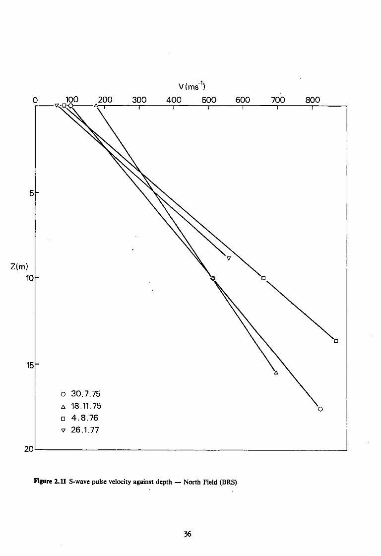
only ± 2 is, indicating a very good fit. The velocities obtained as a
function of depth are shown in figures 2.1H and 2.11. The largest
distance was 40 m corresponding to a depth of 18 m. The mean value of k
was 46 ± 11 s _ 1 and the mean values of V was 109 ± 48 ms-1. Mean o
velocities are shown in Table 2.IB with the standard deviations at various
depths. The latter appear to drop from ± 44% at the surface to a
minimum of ± 7% at about 5 m rising to ± 14% at 11 m depth. The higher
variability near the surface is probably due to larger percentage errors
in timing over short distances. The variation in Vq may be also due to
variability of the fill material in the top metre of the ground.
Errors at greater depths could be due to inhomogeneities in the longer
refraction paths. There did not appear to be any seasonal variation.
The shorter surveys tended to give higher values of k suggesting that
k may decrease with depth.
2.1.2 Site on London clay, Brent
Similar shear wave refraction surveys were made on a site on London clay
close to the North Circular Road at Brent which previously had been
investigated very thoroughly with a programme of plate tests and pile
tests by the Building Research Station (Marsland, 1971) (Cooke and Price,
1973). The results of fitting the data by calculator are given in
Table 2.1C. The average standard error was ± 5 millisecs again showing
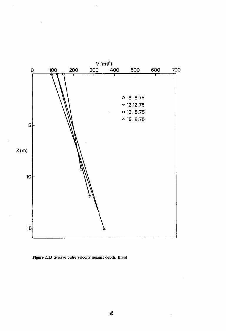
a good fit. In Table 2.ID the spread of velocities at various depths is
given and the standard deviations are only 4 or 5%. The velocities are
shown graphically as a function of depth in figure 2.1J the greatest depth
being 15 m. This was obtained on the survey which was carried out at
night in order to take measurements with a lower background noise level.
35
V(ms"1)
Figure 2.11 S-wave pulse velocity against depth — North Field (BRS)
36

TABLE 2. 1C S-WAVE, BRENT (PULSE)
Date AT millisecs kCs"1) -1 V ms o a Z (m] max
8.8.75 3 9.0 151 0.062 9.3
12.12.75 6 13.0 122 - 0.04 11.9
13.8.76 6 15.0 120 0.002 13.5
19.8.76 6 17.0 96 - 0.34 15.1
Mean 13.5 + 3 122 + 23
TABLE 2.1D MEAN S-WAVE VELOCITIES, BRENT (PULSE)
z(m) V (ms"1)
3 163 + 13
6 203 + 5
9 2 4 4 + 1 0
TABLE 2.1E S-WAVE VELOCITIES, MADINGLEY (PULSE)
Date AT millisecs k Cs"1) V Cms"1) o a Z (m) max
23.3.76 3 12.0 178 0.041 14.2
37
V (ms1)
Figure 2.1J S-wave pulse velocity against depth, Brent
38

2.1.3 Site on Gault clay, Madingley
A shear wave refraction experiment was carried out at the Cambridge
University Civil Engineering Department test site at Madingley. The
results are shown in Table 2.IE and figure 2.IK. The standard error was
± 3 millisecs. Similar velocities were obtained by computer fit although
it was thought that beyond 25 m the time distance curve could be
approximated by a straight line indicating that k could be closer to zero
below 5 m or so. Errors in k were estimated at ± 14% and in V as ± 10%. o
2.1.4 Site on chalk of silos
Two shear wave surveys were made at a site on grade IV to grade V chalk
that carried four large silos of 12 000 tonnes capacity (Burland and
Davidson, 1976) and is the site of an even larger new silo to take 25 000
tonnes.
The surveys were made in opposite directions and the results from curve
fitting are shown as the straight lines in figure 2.1L. One survey gave
an almost zero increase of velocity with depth ie k = 0, while the other
gave a small value of k = 10s""1 with a mean V of 300 ms""1. This was o
consistent with the site investigation that gave grade IV to V chalk to a
considerable depth with some inclusions of grade III and occasionally
grade II. The SPT count remained constant with depth, about an average
value of 11.
For this site the Nimbus seismograph was used with the swing hammers
mounted on a van. Three people carried out the surveys in a single day.
39

V (ms~1)
Figure 2. IK S-wave pulse velocity against depth — Madingley, Cambridge
40

Seismic noise measurements as described in the next chapter confirmed the
shear wave velocity as being close to 300 ms"1 and not increasing much with
depth, see figure 2.1L.
2.1.5 Site on chalk of CERN test tank, Mundford
Shear wave refraction measurements were made on the site of the CERN test
tank at Mundford using the method described in section 2.1. However
because of a surface layer that carried a strong surface wave and the high
shear wave velocities a specific methodology was adopted.
Having set up the van with swing hammers and solid state inertia switches
the strongest reversing shear wave signal was located with the Nimbus
seismograph and tracked across the site with low gain. This gave a
linear plot of arrival time against distance with a low velocity
identified as a surface L-wave in the surface layer of sand.
Then with nearly fifty metres between the swing hammers and the s-wave
geophone the gain was increased and a reversing pulse located with an
arrival time less than half that corresponding to the surface wave. This
was positively identified by measuring the height of the pulse with a
definite number of hammer blows on one side and then seeing that the
height doubled, with an equal number of blows on the opposite side added,
and the geophone polarity switch reversed.
The s-wave pulse was tracked out to 95 m and then back towards the swing
hammers down to 6 m.
41

Figure 2.1L Refraction and seismic noise velocities, Grade IV chalk
42
This procedure helped in positively identifying the s-wave and avoided
the problem with overlap of the three kinds of wave from the source at
short range. It was helped by low background noise levels, thought in
part to be due to the high stiffness of this site, which enabled high
gains to be used. Adding the two sets of reversed pulses meant that
at 48 m a pulse of 20 mm height was seen on the screen of the Nimbus.
The plot of time of pulse arrived against distance is given in
figure 2.1M. This was fitted by equation 1.7 to yield a surface velocity
of 590 ms"1 increasing by a k of 18 s"1 with depth to a maximum depth
of 24.9 m as shown in figure 2.IN. These high shear wave velocities gave
high stiffnesses as described in section 6.2.3.
2.2 Associated p-wave surveys
These were carried out using the standard technique with the Bison seismo-
graph and a p-wave geophone. The source was a 20 kg hammer striking the
ground vertically. Stacking was used for the longer distances and a range
of 60 m was obtained at the North Field BRS corresponding to a depth of
some 25 m (see figure 2.2A). Measurements were also made at Brent and
Madingley (see figure 2.2B). The data was fitted by the calculator
programs and the results are shown in Tables 2.2A. The p-wave velocities
were considerably higher than the s-wave velocities and this ratio made
possible the calculation of the dynamic Poisson's Ratio v from equation 4
shown in Table 2.2B.
At the North Field v drops from 0.47 near the surface to 0.37
at 17 m depth possibly indicating an approach to the lower value
corresponding to the chalk known to be at about 19 m depth. On the
43
150 h
Figure 2.1M Shear wave refraction survey, Mundford
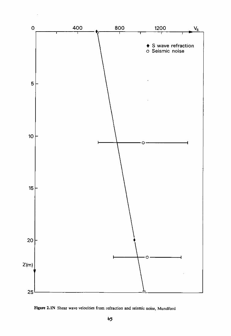
Figure 2. IN Shear wave velocities from refraction and seismic noise, Mundford
Vp (ms1)
Figure 2.2A P wave velocities North Field (BRS) 46

Vp (ms1)

TABLE 2.2A P-WAVE PULSE VELOCITIES
Site Date AT millisecs k (s"1) V (ms"1) o a Z(m) D(m)
N Field 30.7.75 1 38 577 - 0.019 9.9 40
N Field 5.8.75 2 53 473 - 0.04 17.6 50
N Field 20.J1.75 J 38 721 0.10 8.6 40
N Field 20.11.75 2 77 433 - 0.13 24.9 60
Brent 8.8.75 1 36 967 0.14 6.6 40
Cambridge 23.3.76 1 42 1359 0.08 8.5 50
i i V v J - . TABLE 2.2B POISSON'S RATIO V =
Depth Z(m) V ms P V ms V v s V V v VR/V s
0 5 10 15 17.5
433 818 1203 1588 1780
Not
104 309 514 719 822
»th Field
4.16 2.65 2.34 2.21 2.17
0.47 0.42 0.39 0.37 0.37
0.24 0.38 0.43 0.45 0.46
0.95 0.95 0.94 0.94 0.94
0 5
967 1147
Bre
122 190
.nt
7.93 6.04
0.49 0.49
0.13 0.17
0.95 0.95
0 5 8.5
1359 1569 1716
Can
178 238 280
ibridge
7.63 6.59 6.13
0.49 0.49 0.49
0.13 0.15 0.16
0.95 0.95 0.95
( K J h
48

other hand the values of v in the London clay and the Gault are very close
to 0.5, typical of a saturated clay.
Having presented the results the corrections and limitations will now be
discussed.
2.3 Corrections and limits to refraction measurements
2.3.1 Pulse broadening
The refraction experiment uses short pulses from the hammer blows and by
Fourier analysis these are rich in high frequency components. For example
the Fourier transform of a Dirac delta function or spike has a continuous
distribution in frequency. The high frequency components suffer
attenuation that is greater than that of the lower frequencies according
to the law that the attenuation coefficient a of a viscoelastic material
is given by
un qv
where n is the frequency, Q the mechanical quality factor and V the wave
velocity. This means that the pulse changes the proportions of its
Fourier components as it travels through a viscoelastic material. In
effect the pulse changes shape and broadens (Knopoff, 1956). The shape
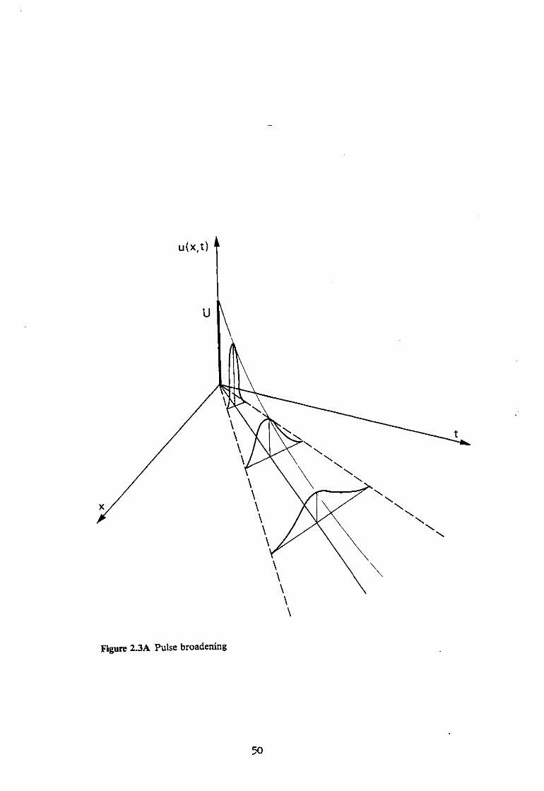
of the pulse is given by
UAx ( 9 x / 2 Vc ) u(x,t) = — 2.1
71 (t-x/V )2 + (9x/2V ) c c
The change of shape with distance is shown by figure 2.3A. Equation 2.1
may be used to calculate the ratio r of the pulse velocity to that of a
continuous wave with velocity c, and 9= 1/Q.
49
u(x,t) *
\
Figure 2.3A Pulse broadening
50
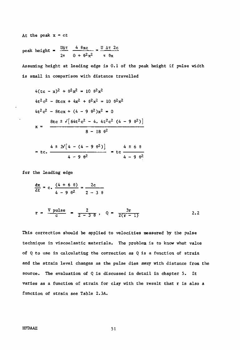
At the peak x = ct
t . t. UAt 4 0xc U At 2c peak height = = 2TT 0 + 02x2 IT 9x
Assuming height at leading edge is 0.1 of the peak height if pulse width
is small in comparison with distance travelled
4(tc - x)2 + 02x2 = 10 02x2
4t2c2 - 8tcx + 4x2 + 02x2 = 10 02x2
4t2c2 - 8tcx + (4 - 9 e2)x2 = 0
8tc ± /[64t2c2 - 4. 4t2c2 (4 - 9 02)] x =
8 - 18 0 2
4 ± 2/[4 - (4 - 9 92)] 4 + 6 8 tc. = tc
4 - 9 02 4 - 9 02
for the leading edge
dx ( 4 + 6 0) 2c _ = c. = a z 4 - 9 02 2 - 3 0
V pulse 2 3r r c 2 - 3 6 ' Q 2(r - 1) 2 , 2
This correction should be applied to velocities measured by the pulse
technique in viscoelastic materials. The problem is to know what value
of Q to use in calculating the correction as Q is a function of strain
and the strain level changes as the pulse dies away with distance from the
source. The evaluation of Q is discussed in detail in chapter 5. It
varies as a function of strain for clay with the result that r is also a
function of strain see Table 2.3A.
HFDAAE 51
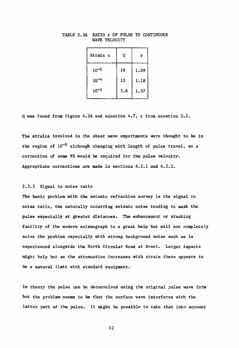
TABLE 2.3A RATIO r OF PULSE TO CONTINUOUS WAVE VELOCITY
Strain e Q r
1CT5 19 1.09
10-4 10 1.18
10"3 5.6 1.37
Q was found from figure 4.2A and equation 4.7, r from equation 2.2.
The strains involved in the shear wave experiments were thought to be in
the region of 10~5 although changing with length of pulse travel, so a
correction of some 9% would be required for the pulse velocity.
Appropriate corrections are made in sections 6.2.1 and 6.2.2.
2.3.2 Signal to noise ratio
The basic problem with the seismic refraction survey is the signal to
noise ratio, the naturally occurring seismic noise tending to mask the
pulse especially at greater distances. The enhancement or stacking
facility of the modern seismograph is a great help but will not completely
solve the problem especially with strong background noise such as is
experienced alongside the North Circular Road at Brent. Larger impacts
might help but as the attenuation increases with strain there appears to
be a natural limit with standard equipment.
In theory the pulse can be deconvolved using the original pulse wave form
but the problem seems to be that the surface wave interferes with the
latter part of the pulse. It might be possible to take that into account
52

as well as allowing for the dispersion of the surface wave but so far this
has not been carried out.
The other aspect of gaining greater depth is related to the general
problem of the inversion of the time distance data to produce information
about the velocity depth profile. It appears that at greater distances
the pulse carries smaller amounts of information about the deeper layers.
This can be seen from the portion of the path at the lower depth,
figure2#1C.In practice the time distance graph flattens out and it is
sometimes difficult to tell whether there is any curvature or whether it
has become a straight line.
2.3.3 Hidden layer
One other point that must be made is that the refraction experiment has
difficulty in the case where there is a high velocity overlaying a low
velocity. In this case the high velocity zone may be missed with a
consequent error in the depths calculated for subsequent layers.
2.4 Surface waves
2.4.1 Rayleigh waves
The second main group of experiments to measure shear wave velocity
involved measurements on surface waves. The most useful type is the
Rayleigh wave which propagates along a surface in a layer approximately
one wavelength deep. The wave velocity VR is close to that of pure
shear waves and differs by about 5% depending on Poisson's ratio (White,
1965).
53

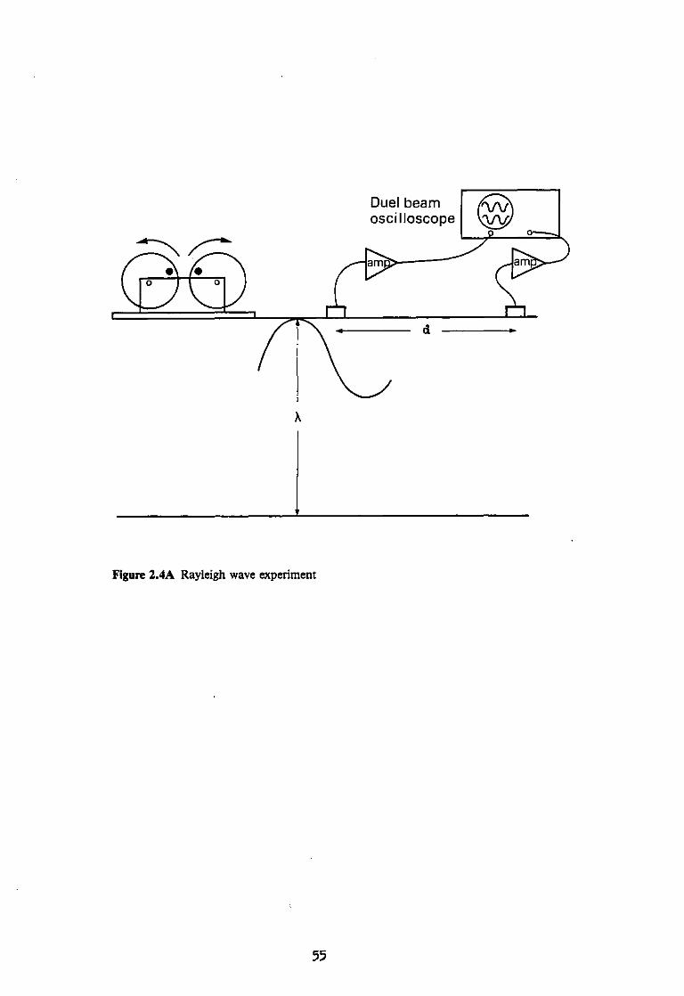
They may be generated by a mechanical or electromagnetic vibrator resting
on the surface of the ground. They are detected by a pair of p-wave
geophones a distance d apart along a line through the centre of the
vibrator, figures 2.4A and 2.4B. The phase angle <j> between the signals
from the two geophones may be measured by a dual beam oscilloscope or a
phase meter. The wavelength X is then given by
The velocity of the Rayleigh waves can then be found knowing the frequency
n from the equation V = nX ,
This may then be corrected to the shear wave velocity using figure 2.4C.
This velocity may be assigned to an average depth of one half wavelength
X/2. In section 2.4.4 it will be shown that this turns out to be a good
approximation and means that measurements near the surface can be made by
higher frequencies and deeper measurements by lower frequencies. The
required depth can in effect be selected by using the appropriate
frequency. This applies even in the case where the refraction experiment
does not work where high velocities overlay low velocities.
A medium sized electromagnetic vibrator was used over the frequency range
30 Hz to 1 kilohertz covering depths from 2 m to a few centimetres below
the surface. It was particularly convenient as the frequency required
could be dialled up electronically. For frequencies below 30 Hz a
mechanical vibrator was used and allowed measurements to be made down to
12 Hz.
54
t
Figure 2.4A Rayleigh wave experiment
55

Figure 2.4B Electromagnetic vibrator and geophones
56

V s / V p
Figure 2.4C V«/V5 as a function of V5/Vp. (White 1965)
57
The phase measurements were made in the first experiments by displaying
the two traces on an oscilloscope screen, photographing the traces and
measuring their relative phase. A much more accurate method was to use a
phase meter such as the Bruel and Kjaer type 2971 which read to one degree
of phase angle even in the presence of background noise.
2.4.2 North Field at BRS
A centrifugal vibrator with contra rotating weights of 0.5 kg driven by
a variable speed electric motor was placed on the surface of the ground,
see figure 2.4D. The base plate in contact with the ground was 0.5 m in
diameter and the whole system was weighed down. The relative positions of
the rotating weights were set so that their effect combined to produce a
vertical simple harmonic motion with no horizontal component, figure 2.4E.
Two sensor type SM4 geophones, vertically polarised, were placed 1.5 m
apart in line with the centre of the vibrator. Signals from the geophones
were amplified by standard ITT audio amplifiers and the signals displayed
on a Hewlett Packard dual beam oscilloscope. Photographs of the traces
were taken with a Polaroid oscilloscope camera. The arrangement is shown
in figure 2.4A.
The speed of the motor was adjusted to produce vibrations over the range
14 Hz to 30 Hz. Relative phase shifts were measured from the photographs
together with the period T = 1/f. Care was taken to allow for the scaling
factor of the photographs.
Higher frequencies were produced by a Ling Dynamics type 400 electro-
magnetic vibrator driving a plate some 200 mm in diameter in contact with
the ground. The device was powered by a Ling type TP0100 oscillator and
58

Figure 2.4D Mechanical vibrator and geophones
Figure 2.4E Rotating weights of vibrator
59

power amplifier and was used over the frequency range 50 Hz to 240 Hz.
At the higher frequencies the geophone spacing was 0.5 m.
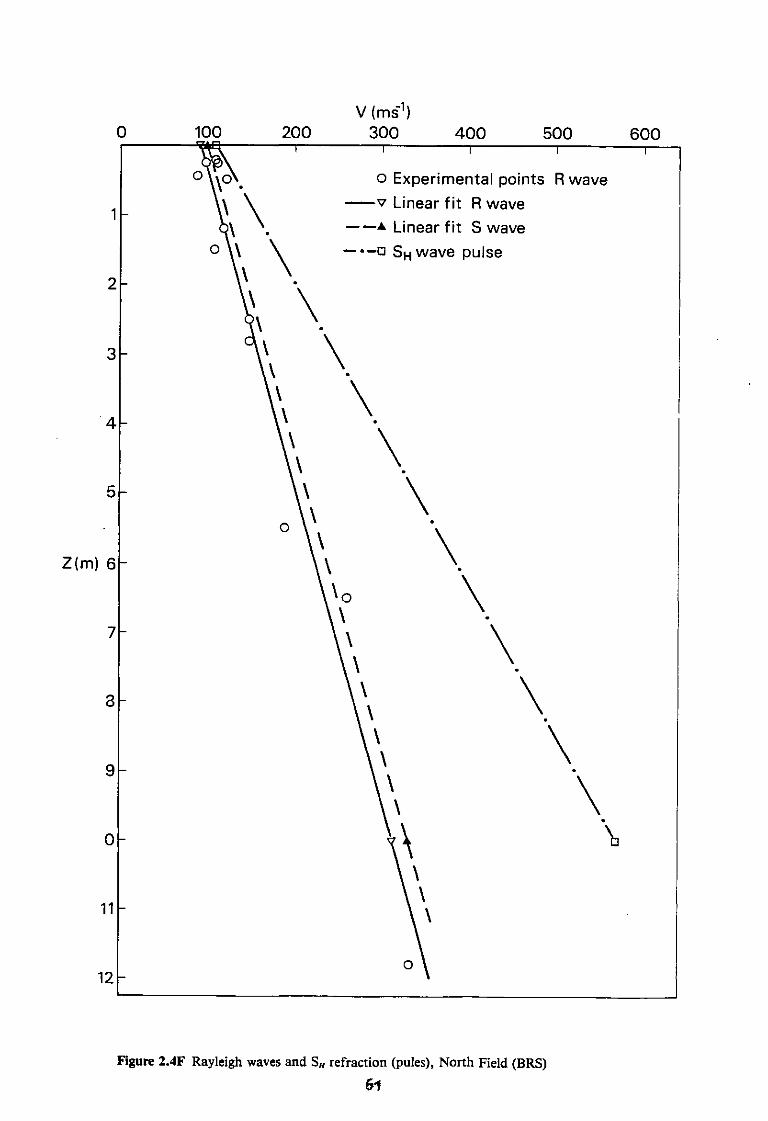
The experimental results are shown in figure 2.4F by the open circles.
They can be fitted by a straight line (shown as a full line) with a
standard error of ± 30 ms"1•
VR = 94 x 22z ms-1 where z was depth down to 11.8 m. 2.3
This was corrected to the shear wave velocity by using the graph given
in figure 2.4C and knowing the ratio Vp/Vg from the p wave and s wave
refraction experiments. This amounted to some 5% so that
V = 99 + 23z ms"1 2.4 s
where z is depth down to 11.8 m. This is shown in figure 2.4F as a dotted
line and may be compared with the results of the s-wave pulse survey
(chain dotted line) obtained from figure 2.11. The refraction survey can
be seen to give higher velocities.
The sources of error were uncertainty in the phase measurements from the
photographs partly due to mechanical noise from gears and non sinusoidal
features in the wave form. In general the phase measurements could be
made to about 10% by this technique. Errors in the time scales of the
oscilloscope were not comparable.
2.4.3 Brent
The same method was used except that measurements were made with the
mechanical vibrator alone. The maximum depth reached here was only 4.7 m
at 12 Hz as shown in figure 2.4G. This was due to the lower velocities
60
V (ms"1) 0 100 200 300 400 500 600
Figure 2.4F Rayleigh waves and S w refraction (pules), North Field (BRS) 6i

V ( m s 1 )
Figure 2.4G V s at Brent
6 2

involved. Experimental points are shown and a linear fit with a standard
error of - 3 ms"1 yielded
V = 73 + 7.2z ms"1 2.5 K and
V = 77 + 7.6z ms"1 2.6 s
These results are compared with the s pulse refraction survey from
figure 2.1J which again is seen to be higher. The same comments apply
regarding accuracy although on this site vibration from traffic was a
problem.
2.4.4 The calculation of depth
The true average depth to which a Rayleigh wave velocity may be assigned
appears to be close to X/2 from several considerations.
Heukelom and Foster (1962) used the depth of X/2 for the corresponding
velocity and could distinguish separate layers of macadam, sand and
gravel and underlying clay. The calculated transitions occurred at the
correct depths. In this experiment it proved possible to measure the
velocities and locate the boundaries in the case where high velocities
overlay lower velocities. This is a situation in which the seismic
refraction experiment does not work. At the Waterways Experiment Station,
Vicksburg in situ velocities have been measured by Raleigh wave methods
using the X/2 relationship (Maxwell and Fry, 1967; Ballard and McLean,
1975). Deep measurements were made by means of very large mechanical
vibrators running at very low frequencies. They were able to locate a
low velocity band within a high velocity region confirmed by other
techniques.
63

The theoretical analysis of Rayleigh wave propagation in layered media is
complicated (Ewing, Jardetsky and Press, 1957). However it can be shown
that for a layer of depth h and velocity Vj_ overlaying a semi-infinite
elastic half space with velocity V2 if A/2<h then the phase velocity tends
to Vi and if A/2>h then the velocity is closer to V2 with a transition in
the region of A/2 = h. This may be seen from the dispersion curves.
There are also finite element solutions for layered media (Lymser, 1970).
These analyses assume that the materials involved are elastic. Horton
(1953) has shown that the effect of viscoelasticity on the velocity of
propagation of Rayleigh waves is small. Borcherdt (1974) also calculated
the velocity of Rayleigh type waves in a viscoelastic material and his
correction even for highly damped cases is small.
An experiment was carried out at BRS which helps to confirm the A/2
relationship as part of work done for British Gas. A pit 1 m deep was
dug and filled with wet mix macadam compacted in layers. Rayleigh wave
velocities were measured using the Ling vibrator and the B & K phase
meter over the frequency range 45 to 200 Hz. Velocities were plotted
against depth A/2 with the result shown in figure 2.4H. A break in the
linear plot of velocity against depth does indeed occur at a depth of 1 m
which would appear to confirm that this relationship is correct in this
situation.
This problem is really an aspect of the general problem of the inversion
of the dispersion curves of velocity against frequency to obtain the
profile of velocity against depth. Seismologists have carried out these
inversions for deep surface waves travelling across continents, by what
64

0 50 100 150 VR(rns~1)
Figure 2.4H Rayleigh wave velocity. Wet mix macadam 65

are effectively iterative computer fitting techniques. Starting from
approximate velocity depth distributions the profile is modified until
a better fit is obtained (Pilant, 1979). The same kind of method could
be used on the smaller scale civil engineering problem and in theory could
deal with a variety of profiles. There are computer programs available to
calculate the dispersion curves (Schwab and Knopoff, 1972).
2.4.5 Transverse surface waves
As well as the vertically polarised Rayleigh waves transversely polarised
surface waves can be produced, these are sometimes known as Love waves.
They were studied by R Jones (1958) and dispersion curves fitted for a two
layer system. This analysis has been extended to multilayer cases
(Cogill, 1974). It does not seem possible to assign a fraction of the
wavelength to an average depth. A considerable amount of work has been
carried out by seismologists to analyse the case of velocity increasing
with depth but the solutions are complicated and have to be tackled
numerically.
In theory the waves could be used to measure horizontal moduli and so by
comparison with the moduli from Rayleigh waves yield anisotropy. However
so far this does not seem to have been attempted. It should be possible
to match observed dispersion curves by appropriate velocity depth
profiles, in a manner similar to that used for Rayleigh waves.
2.4.6 Deep measurements
The problem with the surface wave technique is to obtain deep information.
With the BRS mechanical vibrator the signal to noise ratio is becoming
quite poor by the lower limit of 12 Hz. On some sites this means a depth
66
limit of 5 m. This could be overcome by the construction of large
eccentric weight vibrators at least as large as a fork lift truck
(Cunny and Fry, 1973) but so far this equipment does not exist in the
UK.
Fairly large vibrators have been used by BRS to vibrate dams
(Deinum et al, 1982) but are not very convenient for site work. There
are also hydraulic vibrators now available commercially.
Another approach is to use signal recovery methods to make measurements
on signals which are well below the noise level. Practical possibilities
are thought to be of making measurements on signals 50 dB below the noise
level. One method could be to use the HP 3721A correlator in a signal
recovery mode to produce the correlation between the generated signal
and the signal from a geophone.
A different way of overcoming this problem is to use the naturally
occurring seismic noise itself which contains the low frequencies of
interest. This is described in the next chapter.
A further method is to use the waves produced by impacts. An impact on
the surface of the ground produces surface waves that account for some
68% of the input energy (Miller and Pursey, 1955). A blow from a hammer
will produce a pulse which contains a large number of Fourier components.
These will travel across the surface at different velocities depending
upon the particular dispersion law that holds for that section of the
ground. The pulse will change shape as it travels due to the differing
speeds of the differing frequency components. If the pulse is recorded
67

and analysed the velocities of the different components may be measured.
If the distance is large enough the pulse will be 'dispersed' and can be
divided up into sections with different arrival times and different
frequency contents.
A variation that is used by seismologists recording seismograms from
earthquakes is illustrated by figure 2.41 (Dziewonski and Hales, 1972).
Broad band recordings are made at two well separated stations of a seismic
event outside the line joining the stations. A cross correlogram is made
from the two recordings which is plotted as a function of time delay
between the two stations. The correlogram is analysed for frequency by
taking time samples and presented as a plot of velocity against period.
In this way velocities have been determined to depths of many hundred of
kilometres below the continental United States.
A marine application has been developed recently by the Institute of
Oceanographic Studies (Whitmarsh and Lilwall, 1982). The impact was
produced by dropping overboard a two tonne concrete cylinder that produced
the pulse on the sea floor. This was recorded at some distance and the
recording analysed for dispersion as described. From this a velocity
depth profile was found giving the dynamic shear stiffness as a function
of depth. This experiment was carried out in the deep ocean.
68

SEISMOGRAMS
CTA
4 5
ADE
TRAVEL TIME
50 55 60 MIN
CROSS-CORRELOGRAM
I - — — j \ l (WWW
10 15 MIN
PHASE VELOCITY
km/sec 5.0h
4.5
4 . 0
3.5
PHASE DIFFERENCES
100 200 PERIOD (SEC)
km/sec 5.0h
4.5
CROSS-CORRELOGRAM
4 .0
3.5 _i L 100 200
PERIOD (SEC)
Figure 2.41 Seismic velocities derived from cross correlogram (Dziewonski and Hales 1972)
69

CHAPTER 3
SEISMIC NOISE METHOD
3.1 Advantages of using seismic noise
Seismic noise appears to be present at the surface of the earth in varying
degrees. It is familiar as a background signal when carrying out seismic
refraction surveys and similar geophysical measurements. The source of
this noise appears to be partly atmospheric, the wind in the trees for
example, conversion of airborne sound and pressure variations to
vibrations in the ground, and partly vehicle movements and even phenomena
like waves breaking on the seashore.
Making measurements from the seismic noise has the advantage that one is
not trying to improve a signal to noise ratio, the measurements being
on the noise itself. The levels of vibration are of the order of atomic
spacings but are easily amplified with modern operational amplifiers
giving high gain at frequencies down to DC. The actual amplitude of the
signal in the geophones may be only a few microvolts but this may be
amplified readily, recorded and then played back as a signal of some volts
amplitude. Some research workers have Fourier analysed these signals and
estimated geotechnical properties from the frequency distribution
(Rousopoulos, 1978).
Most seismic noise is thought to be in the form of surface waves
travelling in a layer one wavelength deep (Iyer and Hitchcock, 1976).
There are also theoretical predictions suggesting that the majority of the
energy (some 68 per cent) from a surface impact goes into surface waves
(Miller and Pursey, 1954; Mooney, 1974). If it is in the form of these
HFDAAF 70

surface or Rayleigh waves then there is good evidence that these waves do
indeed travel in a surface layer one wavelength deep (Woods and Richart,
1967) and the vertically aligned geophones should not pick up the
horizontally polarised Love waves.
The frequencies of seismic noise lie in the range of from about 1 Hz to
50 Hz. With shear wave velocities in the region of 100 to 700 ms-1 the
corresponding wavelengths and depths range from one or two metres down
to 100 m. This range satisfies the requirements of most civil engineering
geotechnical problems. Since acoustic surface waves are already there and
do not have to be generated they may be used with advantage in some circum-
stances, for example on the sea floor (Bradner, Dodds and Foulks, 1965).
By filtering the signals with moderate selectivity, waves corresponding
to a particular depth range may be chosen. If the geophones are arranged
in a triangular array and broadband signals recorded then correlation
measurements will reveal the delays along each side of the triangle for a
particular frequency. Using vector methods the direction and velocity may
be deduced for the particular sample of the record that is being examined.
Knowing the velocity and frequency a wavelength may be found and so the
depth corresponding to that velocity deduced. The method is very similar
to the standard Rayleigh wave technique except for the source being broad-
band in frequency and the direction being initially unknown but deduced
from the delays on the arm of the array.
That correlation techniques can be used for measuring surface wave
velocities has been demonstrated by Roesler (1978). Filtered 'white
71

noisef signals were applied to an electromagnetic vibrator and the
correlation observed with a signal transmitted through the ground and
detected by a geophone.
3.1.1 Correlation techniques
Correlation methods may be used to determine the delay between the arrival
of a signal In two channels. This signal may be discrete or continuous.
A correlator displays the integral
T c ( X ) = / V1 (t) V2 (t - T) d t 3.1
o
of the product of the two voltages Vi and V2 with V2 delayed relative to
Vi by x where T is the sample time. If the signal is delayed in one
channel relative to the other by T^ then there will be a peak in c(x) at
x = Tx. If it is a continuous sinusoidal signal then c(x) will be a
sinusoid with the same period Tp as the original signal but with a phase
shift relative to x = 0 of
Ti <j) = — x 360°
P
Thus the phase shift may be read off the correlator directly. This will
work even in the presence of uncorrelated random noise which will not
contribute to the correlation function c(x) as the correlation between two
truly random signals is zero.
The instrument used for the observations reported in this thesis was a
Hewlett Packard 3721A correlator. It has the advantage of being able to
calculate the correlation function rapidly from digitally stored samples
72

of the signals. The calculated function is displayed on the screen of a
cathode ray tube.
The correlation curves found from the seismic noise tended to be fairly
long wave trains, varying in amplitude, and decaying over a period of
seconds in some cases. Thus the measurement taken was in fact the time
Ti of the first peak of a decaying sinusoidal curve (figure 3.1A). The
noise is thought in some ways to be similar to the swell on the surface
of the sea.
3.2 The method
3.2.1 Filtering
In order to select the frequencies which are required for the correlation
measurements the signals need to be filtered before the correlation is
carried out. Ideally filters that produce no phase shift would be used
(Kulhanek, 1976).
There is a fundamental problem involved in this process which is akin
to the 'uncertainty principle' in quantum mechanics. The filtering must
not be too tight or accuracy will be lost in time measurements. This
follows from the behaviour of Fourier transforms. The transform of a
wave packet is a spread group of frequency components whose breadth is
inversely proportional to the width of the packet in time.
Thus A t A n = 1 3.2
In this study active filters made from operational amplifiers were used
producing the normal phase shifts as a function of frequency. However,
73

AVERAGING m ) f RMS VOLTS 1 V I RANGE A
V y ^ v A . J - A .
PflOBABiUTY A NPUT
EXPONENTIAL
r
Figure 3.1A Correlation curve on screen of correlator
74
the phase shift for the centre frequency was thought to be approximately
zero and the correlator displayed a trace that corresponded to this centre
frequency. A correction was applied for a difference in phase shift or
time delay between the two filters employed.
The width of the filter band was such that the Q was approximately unity
(Q = An/n, where An is the breadth of the pass band at the 0.707 of
maximum amplitude points). This appeared to be a satisfactory compromise
that gave sufficiently tight filtering with sufficient accuracy in the
measurement of time delays.
3.2.2 The geophone array and calculations of velocity
The noise wave packets could come from any direction and so signals were
recorded by an equilateral triangular array which contained three
geophones. The lengths of the sides of the triangle were chosen so that
the delays were a reasonable fraction of the period of the middle
frequency.
In practice with long wave trains it was not possible to distinguish
between forward and backward travelling waves. In other words, the delay
time might have been T or T - T^ see figure 3.2A, where T was the time of
the first peak observed on the correlator screen. This meant that there
were only six possible combinations of times to be used in the solution
of the following equations, see Table 3.2A.
75
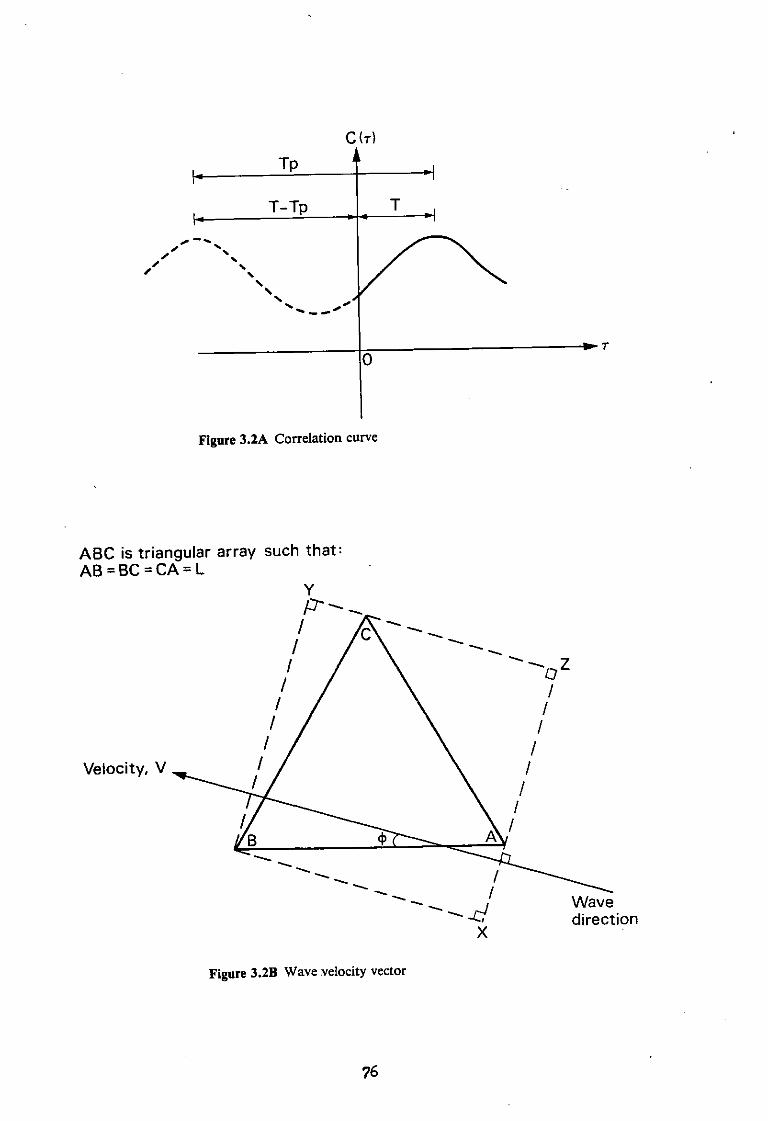
C(T)
ABC is triangular array such that : AB = BC = CA = L
Y
Figure 3.2B Wave velocity vector
76

TABLE 3.2A
Angle Time delays I
30 < * < 90 T AB T T - T P 1
-30 < * < 30 T AB T -BC T P T -CA T P 2
270 < • < 330 T AB T -BC T P T CA 3
210 < • < 270 T -AB T P T -BC T P T CA 4
150 < <J> < 210 T -AB T P T BC T CA 5
90 < * < 150 T -AB T P T BC T -CA T P 6
A calculator program reduced the number of possibilities to one for the
following reasons.
From figure 3.2B XB = L cos 4 3.3
CY = -L cos (120 - 4) 3.4
ZC = -L cos (240 - +) 3.5
The delays observed by going round the triangle cyclically were
T T T AB> BC' CA*
.T XB —CY _ ZC _ r N o w TAB • — • TBC - v" ' TCA = - V" 3 , 6
Hence L cos 4 _ L cos (120 - 4) _ L cos (240 - 4)
y - m — — J • / m m m AB XBC CA
These equations may be solved for V and 4*
There are six possible solutions listed in Table 3.2A with 4 in six
possible ranges of angle. The correct solution is identified with the
77

calculator program by first noting that T^g + TgC + T C A = £t should sum to
zero. This can be seen from equation 3.6 which gives
r. XB CY ZC IT = — - — - — = 0 as XB = ZC + CY
In practice the sums of the times for the even values of I will add to
one figure and the sums of the times for odd values of I will add to
another different result. Thus the correct choice of the odd set or the
even set may be made on the basis of the one that gives the lowest IT
(taking signs into account). This reduces the number of possibilities
from six to three. Of these three possibilities a choice is made of
the one for which the velocity deduced is the fastest, or in other words
the solution for <j> which gives £|T| a minimum (ie not taking signs into
account).
This choice is justified by the relationships shown in figure 3.2B.
Provided that AB < X/2, then T ^ < Tp/2 and T ^ < Tp - T ^ , so the correct
choice between T^g and (T - T^g) is the smaller of the two, T^g.
The two possibilities for side BC are now T ^ cos + 60) and Tp - T ^
cos (<|> + 60). As cos (<{> + 60) is for <j> <90 the choice of this pair is
even more strongly the smaller of the two.
A similar argument applies to side CA. The choice is now to be made
between T^g cos (60 - <J>) and Tp - T^g cos (60 - <j>) and again as cos
(60 - <j>) <1 for <j> <90 the correct time is the smaller T ^ cos (60 - <j>).
With the smaller time for each side, IlT| is a minimum provided that
AB < X/2.
78

This argument for the reduction of the three possibilities to one choice
applies whichever side the wave direction is closest to, ie <j) may refer to
AB, BC or CA. As a result the array can only be used to deduce velocities
at depths greater than L, the length of the side of the array, using the
interpretation of section 3.2.6.
3.2.3 The recording system
Three geophones were placed at the corners of an equilateral triangle of
side 5 m. These marine geophones were made by Sensor of the Netherlands
and gimbal mounted so that they would align themselves vertically over a
range of 180°. Their frequency response went down to 10 Hz.
The geophones were attached to 20 m of waterproof cable which led to pairs
of operational amplifiers connected in series to provide high gain. The
high input impedance of the amplifiers reduced the effects of the length
of cable. The DC levels could be adjusted to zero by a fine control and
the outputs to the tape recorder were through attenuators so that the
correct recording level of less than 25 mV could be maintained. The
signals were observed via a Philips PM 3233 dual beam oscilloscope. The
three seismic channels were recorded on an Oxford Instruments Microlog
recorder fitted with AM5 preampifiers that gave a frequency response from
DC to 50 Hz. A one second pulse from an integrated circuit timer was
recorded on the fourth channel. Care was taken to see that this pulse was
symmetrical above and below zero volts. The amplifiers, timer and
recorder all fitted in a small box some 290 mm x 200 mm x 150 mm as shown
in figure 3.2C. The readings were made on standard C90 cassettes.
79

Figure 3.2C Recording system showing one geophone in holder
Figure 3.2D Equipment for analysis of signals
80

3.2.4 Analysis system
The tapes were played back by an Oxford Instruments PB-3 playback unit.
Two of the seismic channels at a time were fed through filters. These
were active filters constructed from an Analog Devices integrated circuit
type FLT-U2 consisting of four operational amplifiers. They could be
switched over a frequency range from 7 Hz to 50 Hz.
The filtered signals were then fed to the two inputs of a Hewlett Packard
type 3721A correlator, see figure 3.2D. This was operated in the cross
correlation mode taking 1 x 1024 samples. A scale setting of 10 ms per cm
gave a sample period of one second, thought to be an optimum time for a
sample, as sufficient information was obtained to find good correlation.
The time was also short enough for the sample to be reasonably easily
located in one wave packet. The criterion applied to ensure that it was
indeed one wave packet was that the correlation curves should grow
monatonically and did not shift peak position in the process.
The correlation curves were damped sinusoids with maximum amplitude at
the first peak. The time of the first peak, T ^ , was noted. The period
was also recorded and checked to see that it corresponded with the
inverse of the filter frequency. The other two pairs of channels were
taken in cyclic order for the same section of tape giving values of
TBC a n d TCA*
The tape playback was under automatic control from a control unit
activated by the timing pulses on the fourth channel. Thus, once the
tape direction had been selected the sequence was initiated by pressing
a start button on the control unit. The correlator was then automatically
81

cleared and the playback unit switched on. When switching transients had
died away the correlation calculation was started by a pulse on the tape.
When the calculation was complete another pulse switched off the playback
unit. The procedure was repeated with the reverse direction selected
to bring the tape back to its original starting point. The next pair of
channels was then selected and the second delay measured for exactly the
same part of the recording defined by the time markers. The third delay
was then found for the third pair. The equipment is shown on figure 3.2D.
Circuits are shown in Appendix 2.
3.2.5 Interpretation
Frequencies n were chosen which corresponded to depths from 3 m to 25 m
with velocities in the range 100 to 700 ms"1. With velocities given by
the calculator program the wavelengths X could be evaluated from the
equation
V = nX 3.8
On the assumption that waves of seismic noise are indeed Rayleigh waves
travelling in a layer one wavelength deep the velocity was assigned to an
average depth of one half wavelength, and V was plotted against depth as
shown in figures 3.2E to 3.2G. A correction was applied to obtain the
shear wave velocity from the Rayleigh wave velocity using an estimated
value of Poisson's ratio. This amounted to an increase of some 4 to 5
per cent.
82
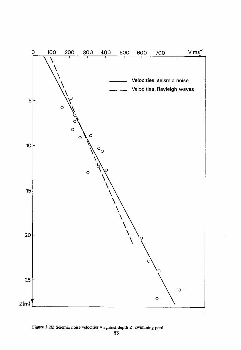
0 100 200 300 400 500 600 700 V ms"1
Figure 3.2E Seiemic noise velocities v against depth Z, swimming pool
83

Figure 3.2F Seismic noise velocities v against depth Z, Brent
84

0 100 200 300 400 500 600 700 V ms"1
Figure 3.2G Seismic noise velocities v against depth Z, Christchurch bay
85

3.3 Measurements
3.3.1 Site on Boulder clay, swimming pool at Bricket Wood
As a trial underwater experiment the geophone array was placed on the
concrete floor of an outdoor swimming pool under approximately two metres
of water. The geophones were positioned by an aluminium frame of 5 m
side. They were attached to the frame by nylon cords which could be cut
by electrically operated explosive cutters leaving the frame to float
free on buoyancy tanks. Seismic recordings were made for twenty minutes.
The site was on Boulder clay a few hundred metres away from BRS where
measurements had been made earlier using Rayleigh waves generated by a
mechanical vibrator. Allowing for the fact that the bottom of the pool
was 1 m below the surface of the ground a good comparison was obtained
between the two methods, see figure 3.2E. This confirms that the noise
was in the form of Rayleigh waves. The seismic noise experiment yielded
V = 52.4 + 27.7Z ms"1 with a mean standard deviation of 15 per cent s compared with
Vg = 94.0 + 22Z ms"1 from the Rayleigh wave experiment shown in
in figure 6, with Z the depth in metres, to
27 m depth.
3.3.2 Site on London clay, Brent
A three metre geophone array was set out on the surface of the London clay
at the BRS test site at Brent in North London and readings made for ten
minutes. A further recording was made with an array of 1 m side. The
results are shown in figure 3.2F. The best straight line through the
results was:
HFDAAG 86

V = 121 + 21Z with an average standard deviation of ± 9 per cent s to 16 m depth.
Again the shear wave velocities were found from the Rayleigh wave
velocities.
3.3.3 Marine site on Barton clay at Christchurch Bay
At this site it was necessary to devise a means of lowering the geophones
from a boat so that they settled on the seafloor about 8 m below the
surface of the water at the vertices of a 5 m equilateral triangle. After
testing various methods, a triangular steel Dexion frame of side slightly
greater than 5 m was constructed. Cylindrical steel holders for the
geophones were hung from the corners of the frame by nylon cord as shown
in figure 3.3A. These cords were to be cut by electrically operated
explosive cutters activated by a twelve volt battery on board the boat.
The cutters were all wired in parallel and their power lines were tied
together with the three geophone cables so that in effect only one line
was brought from the seafloor to the boat.
The steel holders gave the geophones more ballast to ensure that they
remained in position on the seabed. Where the geophone cables came
together a fifteen kilogram weight was tied to prevent them from swaying
in the current. The cables were made to run under the frame so that they
would not he disturbed when the frame was lifted away.
Ropes tied to the corners of the frame became a single line after a length
of five metres or so. The frame and weight were lowered over the side of
the boat onto the seafloor using a single line.
87
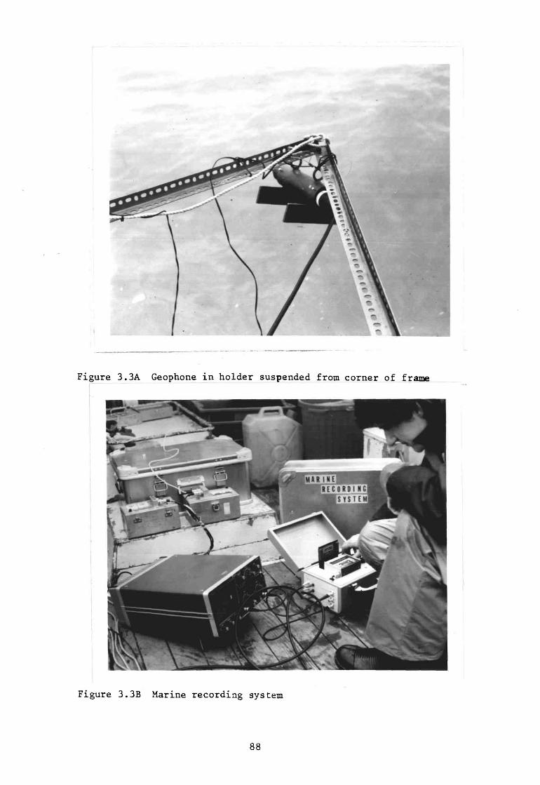
Figure 3.3A Geophone in holder suspended from corner of frame
Figure 3.3B Marine recording system
88

Care had to be taken that the weight and frame were lowered together so
that no force put undue strain on the geophone cables.
This operation needed the efforts of three people but was carried out with
relative ease.
Once the geophones were on the seafloor, the cutters were activated and
the frame pulled away and secured to the boat. Readings of the seismic
noise were then made, see figure 3.3B, which shows the recording equipment.
The results are shown in figure 3.2G where Vg = 4.5 + 31.OZ ms-1 with an
average standard deviation of ± 11 per cent to 15 m depth.
3.3.4 Site on chalk of silos
For the measurements described in sections 3.3.4 and 3.3.5 the equipment
was modified to operate over a higher frequency range 10 Hz to 500 Hz.
This involved a change of the recorder and playback units to an amplitude
modulated (AM) system. Amplifiers in the tape recorder and playback unit
were changed over and the playback tape speed increased by a factor of
five. Resistors in the filter units were also changed by appropriate
amounts to select frequencies in the new playback range.
Other modifications required were the alteration of the pulse timer
circuit to produce a train of 32 pulses every other second. CMOS
(complementary metal oxide semiconductor) integrated circuits were used to
reduce current drain in the field. The playback control unit was modified
to respond to this pattern of time markers. It was required because the
switch on and switch off times of the playback unit were now quite long in
relation to the pulse period. Additional counting circuits were added to
89
the controller. Calibrated attenuators were fitted to the recorder so
that levels of recording could be interpreted in terms of amplitude.
The new system was checked on the North Field at BRS where a recording
was made and values of velocity as a function of depth obtained that were
close to those found with the earlier pulse width modulation system.
At the site of the silos the triangular array was set out approximately
in the centre of the line of the shear wave survey and the recording run
for twenty minutes.
The tape was played back using a new switching system that selected pairs
of channels in cyclic sequence. The noise recording was found to contain
frequencies mainly close to 10 Hz in real time almost to the exclusion of
other frequencies. This meant that only one point could be obtained as
shown in figure 2.1L at a depth of 12.5 m giving a velocity of
295 ms-1 ± 17%.
While carrying out this experiment it was realised that for each frequency
analysed, or point plotted on the graph of velocity against depth,
individual readings would lie on a line through the mean point and the
origin as shown in figure 2.1L by the dotted line. The standard deviation
then corresponds to all readings obtained at that frequency.
The presence of a noise signal predominantly at 10 Hz was thought to be
due to a foundation resonance of the silos being at a much higher level
than the background noise. Detailed spectral analysis by spectrum
analyser or Fourier transformation should yield information about the
foundation behaviour.
90

The value of velocity was quite close to that of the shear wave refraction
apparently showing that the site did not increase much in stiffness with
depth for the first 12 m.
3.3.5 Site on chalk of CERN test tank, Mundford
Recordings were made of the seismic noise at this site using the AM
system with triangular arrays of both 5 m and 10 m length of side. The
noise level was low so that relatively high gain settings of the
attenuators were required. Frequencies were also higher than on other
sites which was the reason for the development of the AM system.
The recordings were analysed as described in the previous section. Two
points, at 10.6 m and 21.6 m, are shown in figure 2.IN. As can be seen
the standard deviation overlaps the line from the shear wave survey. The
value of the standard deviation for the upper point was ± 42% while for
the lower point it was ± 30%. The reason for this level of uncertainty
was thought to be the increased proportion of timing error in relation to
reduced delay times with these higher velocities. However the 10 m array
did not seem to give a better accuracy than the 5 m array.
A third point is shown in figure 3.3C at 32 m depth being the deepest
point obtained by this method.
The experiment shows that a proportion of microseismic noise is in the
form of surface or Rayleigh waves. Seismic noise may be used to determine
the variation of shear wave velocity with depth. The great advantage of
the technique is that deep measurements may be made without large
vibration generators.
91
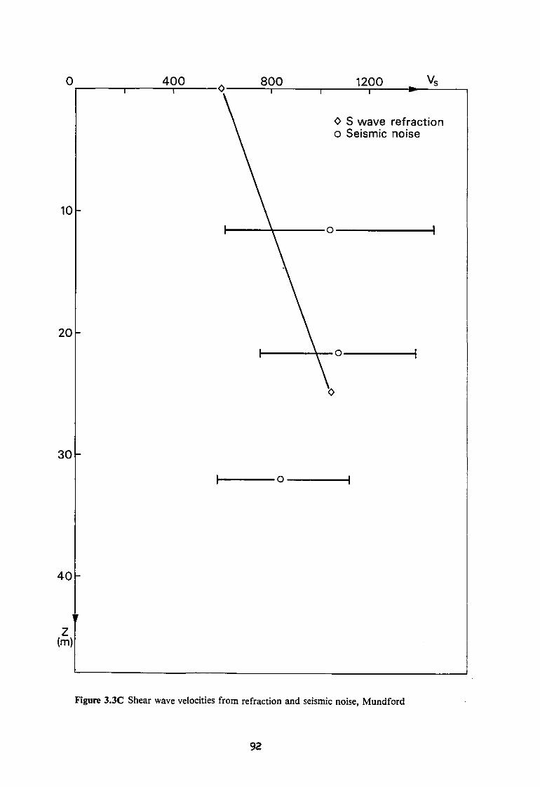
Figure 3.3C Shear wave velocities from refraction and seismic noise, Mundford
92

CHAPTER 4
TIME AND STRAIN DEPENDENCE OF MODULUS
4.1 Time dependence
Up to this point the study has been devoted to the measurement of the
velocity of shear waves in the ground. For this information to be useful
the relationship must be found between shear wave velocity and the static
stiffness, or modulus, of the ground. As described in section 1.5 for a
perfectly elastic material the relationship between shear wave velocity
and shear modulus is given quite simply by
However the ground is not perfectly elastic. For real soils the stress
strain behaviour is non linear and time dependent. For most soils the
non linearity reflects plastic behaviour (ie irrecoverable strains). At
low strains plastic behaviour can be ignored and the soil skeleton can be
assumed to be non linear viscoelastic.
In the first part of this chapter the time dependence of the modulus will
be discussed and in the second part the non linear behaviour of the soil
will be examined.
4.1.1 Theory
Time dependent behaviour may be observed in two main types of experimental
situation. In the first a constant stress or strain is applied, and the
resulting time varying strain or stress observed. The generalised Hookes
Law of equation 1.2 then applies. A time dependent compliance J(t) is
defined corresponding to a constant stress a
G = pVg2 1.4
e(t) = J(t) oQ, J(t) = i [l + 4>(t)] 4.1
HFDAAH 93

This is the quantity that is of interest from a geotechnical point of view
as stresses are usually fairly constant as in the case of dead loading and
the strains show the time dependent behaviour of creep (see figure 4.1A).
There is also a time dependent modulus M(t) at constant strain which gives
the relaxation or variation of stress required in order to maintain a
constant strain
a(t) = M(t) eQ 4.2
The second, dynamic situation on the other hand where a sinusoidal stress
a(u>) is applied, corresponds to the case of the geophysical shear wave
measurements, to is the angular frequency, ui = 2irf where f is the normal
frequency. Now the stress strain relationships become
e(u)) = J*(w) a (a)) 4.3
a(u>) = M*(u>) e (ai) 4.4
where J*(W) and M*(OJ) are the complex compliance and modulus respectively
that are required to produce the appropriate amplitudes and phase shifts,
as discussed in Nowick and Berry (1972). The strain in equation 4.3 lags
the applied stress by a phase angle dependent upon the viscoelastic
damping of the material.
If the material is perfectly elastic then J(t) = J* = J the compliance,
and M(t) = M* = M and J = 1/M, and the material is not time dependent.
However, with time dependent processes occurring in the material the
behaviour defined by equation 4.1 in response to a step function in
applied stress may be as shown in 4.1A.
94
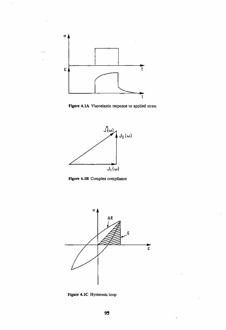
Figure 4.1 A Viscoelastic response to applied stress
Figure 4. IB Complex compliance
Figure 4.1C Hysteresis loop
95

In many civil engineering contexts the requirement is to be able to find
the strain when known stresses are applied. To this end it is convenient
to work with the compliance J instead of the modulus M, as the strain is
simply the stress multiplied by the compliance as in equation 4.3. If
complex the appropriate phase shifts will be produced.
The complex compliance J (u>) may be expressed as J^(10) + j J2(uj), see
figure 4.IB where j is the square root of -1, Jx(OJ) is the real part and
J2(t»>) the imaginary part. Both J i ( w ) and J 2 (<o) may be a function of
frequency. J (w) is the vector sum of the two components Ji(w) and J2(w)
and may thus be represented vectorially in the same way as electrical
quantities where the real and imaginary parts are referred to as resistive
and reactive.
4.1.2 Damping
The additional quantity that is required besides a measurement of the
elasticity is the damping. This is found to relate to the time dependent
behaviour of the material both in the context of creep and the phase
shifts in the dynamic situation.
Definitions of damping vary. For the purposes of this thesis, we define
the damping factor, 1/Q, as the ratio of the energy lost per cycle, AE, to
the energy stored per cycle, E, divided by 2ir. In figure 4.1C a typical
hystereses loop is shown.
i = i - ^ 4 5 Q 2tt E °
AE is the area within the loop and E is the area of the shaded triangle.
96

Q is the mechanical quality factor analogous to the electrical quality
factor, also given the symbol Q, which is the measure of the sharpness
of the resonance in a circuit. For materials normally considered to be
elastic such as metals and crystals, Q is high 103 or higher, but for
some earth materials it may be below 10 and so damping must be taken into
account.
There are several other quantities that are used to measure damping. The
logarithmic decrement, 6, is defined as
Al 5 = In — 4.6 A2
where Ai and A2 are successive amplitudes of a vibration damped by a
material, see figure 4.ID.
Alternatively, if the material is part of a resonant system with a
resonant frequency at OJQ then the bandwidth of the O.IOTA^^ points,
^-(Di, is another measure, see figure 4.IE.
A further quantity found in the literature is the damping ratio, D, which
is the ratio of actual damping to the critical damping. Critical damping
is the value of the damping where the solution to the differential
equation governing the vibration changes from an oscillatory solution to
an exponential decay. D is usually deduced via equations 4.5 and 4.7 and
this critical damping is the value of D for which AE = 4irE.
The quantities are related approximately as
i 5 w2-u>x = 2D 4.7 0) o
97

Figure 4.1E Broadening of resonance peak
98
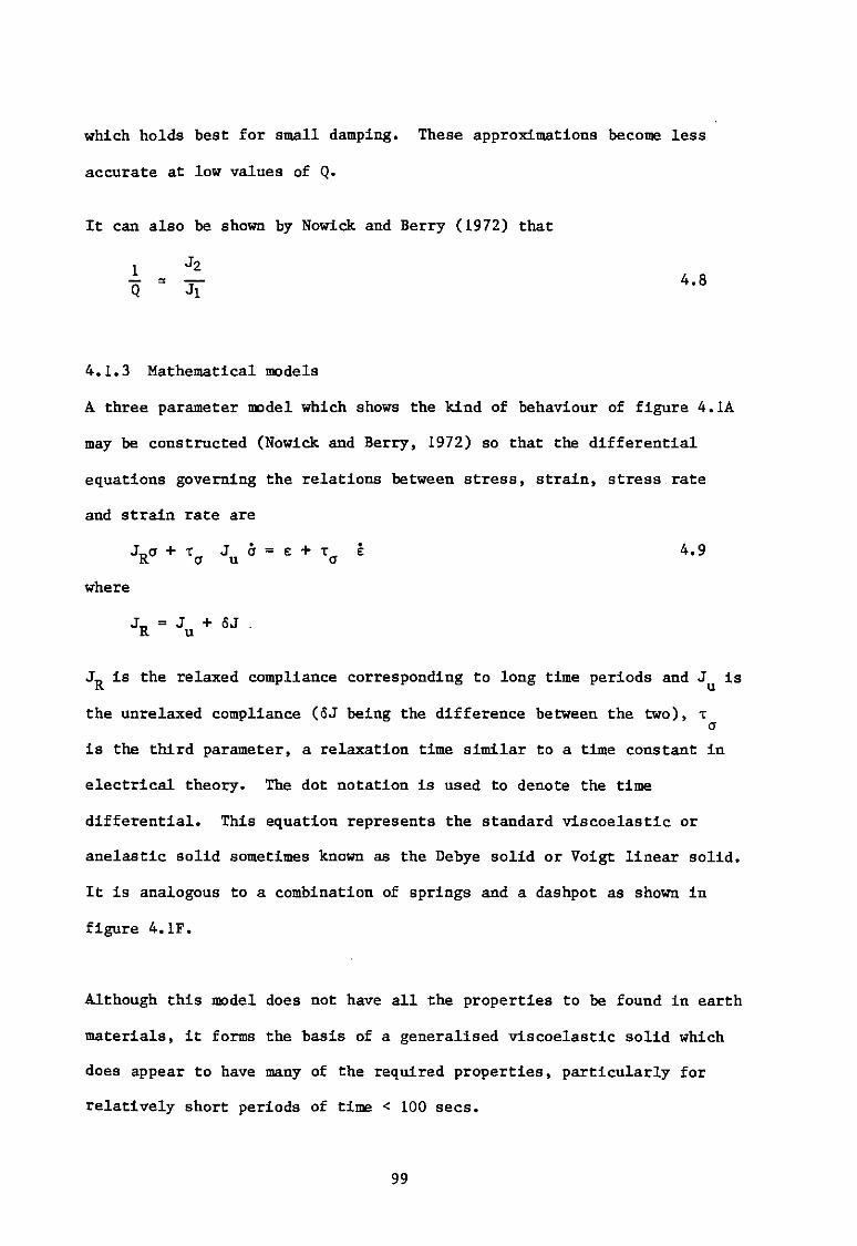
which holds best for small damping. These approximations become less
accurate at low values of Q.
It can also be shown by Nowick and Berry (1972) that
4.1.3 Mathematical models
A three parameter model which shows the kind of behaviour of figure 4.1A
may be constructed (Nowick and Berry, 1972) so that the differential
equations governing the relations between stress, strain, stress rate
and strain rate are
J„a + T J c r = E + T E 4.9 R a u a where
J„ = J + 6J . R u
J^ is the relaxed compliance corresponding to long time periods and J^ is
the unrelaxed compliance (5J being the difference between the two), T a
Is the third parameter, a relaxation time similar to a time constant in
electrical theory. The dot notation is used to denote the time
differential. This equation represents the standard viscoelastic or
anelastic solid sometimes known as the Debye solid or Voigt linear solid.
It is analogous to a combination of springs and a dashpot as shown in
figure 4.IF.
Although this model does not have all the properties to be found in earth
materials, it forms the basis of a generalised viscoelastic solid which
does appear to have many of the required properties, particularly for
relatively short periods of time < 100 sees.
99
(b) 6J TCT
6J (C)
(a) 'u
Figure 4. IF The standard viscoelastic solid
100

The time dependent compliance, J(t), can be shown to be a solution of
equation 4.9 of the form
J(t) = Ju + 6J[l - exp(-t/xa )J 4.10
which shows the exponential creep behaviour of figure 4.1A. If a periodic
stress is applied corresponding to the case of dynamic measurements, then
0 = 0 e^wt o
where OQ is the maximum amplitude of a. The real part of a is a
sinusoidally varying term.
The resultant strain consists of a sinusoidal term shifted in phase with
respect to the applied stress and represented by
e = (ei-j£2)ejwt 4.11
£l being the strain component in phase with the applied stress and £2 the
component with a 90° lag.
The components of the complex compliance are now
ex e2 Ji = — and Jo = — 1 o * o o o
The explicit forms of the expressions for these quantities are given in
Appendix 1 and are known as the Debye equations. These have a transition
in Jx and a peak in J2 centred on a frequency 1/(2tt x ). The range of
the effects of these transitions is limited to approximately ± 1 cycle in
log frequency.
The range of the transition needs to be extended as found in practice.
This can be done by allowing J R to be comprised of a series of discrete
101
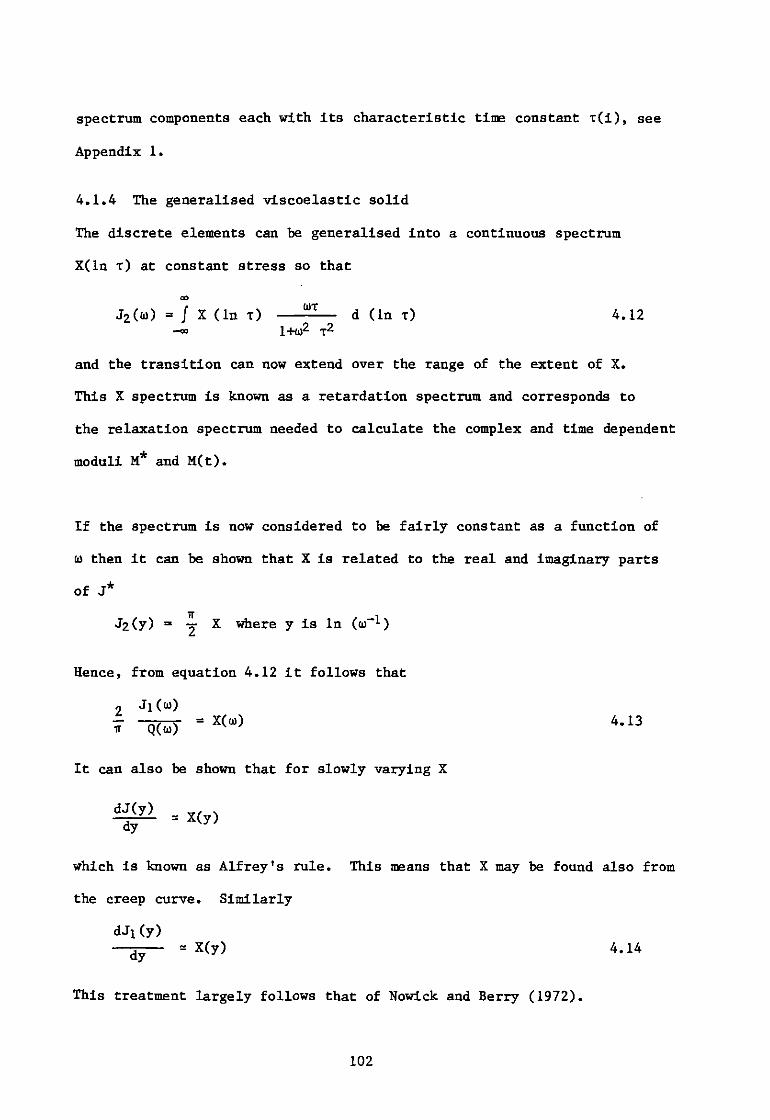
spectrum components each with its characteristic time constant x(i), see
Appendix 1.
4.1.4 The generalised viscoelastic solid
The discrete elements can be generalised into a continuous spectrum
X(ln T) at constant stress so that
00 J2(o>) = / X (In T) — — d (In x) 4.12
-« L+O)2 X 2
and the transition can now extend over the range of the extent of X.
This X spectrum is known as a retardation spectrum and corresponds to
the relaxation spectrum needed to calculate the complex and time dependent
moduli M* and M(t).
If the spectrum is now considered to be fairly constant as a function of
a) then it can be shown that X is related to the real and imaginary parts r* of JJ
J2(y) = y X where y is In (aT1)
Hence, from equation 4.12 it follows that
2 Jl(w) — x = X(co) 4.13 IT Q(o>)
It can also be shown that for slowly varying X
which is known as Alfrey's rule. This means that X may be found also from
the creep curve. Similarly
dJi(y) * X(y) 4.14 dy
This treatment largely follows that of Nowick and Berry (1972).
102

By combining equations 4.13 and 4.14 we find
_L dJ(y) . 2 1 J(y) dy TT Q 4 . 1 5
and the creep rate is seen to be proportional to the damping factor. This
may be compared with the similar results of Lomnitz (1956), (1957) and
If X(y) is reasonably constant and using the approximation that M = 1/J
we find the time dependence of the modulus is given by
where t and t2 are two different periods of time.
4.2 Strain dependence
4.2.1 Effect of non linearity
The foregoing analysis assumes that the damping 1/Q is independent of
strain. In fact, for a clay the damping is found experimentally to
increase with strain see figure 4.2A (Bolton Seed and Idriss 1970;
Hardin and Drnevich, 1972). The variation of damping factor with strain
is not large, the maximum change being a factor of two over a range of
strain of ten. In addition, the modulus decreases with increasing strain.
Thus, the damping should be measured as a function of strain and the
appropriate value used to calculate the creep term or the time dependent
correction. For a low strain situation, the low strain value of damping
is used and the strain dependence only becomes of importance when
extending the analysis to higher strains.
(1974).
ti \ 2/TTQ 4.16
103

o 4f D(%)
Strain (%)
Figure 4.2A Damping ratios for saturated clays, from Bolton Seed and Idriss

The analysis for linear viscoelastic materials can be seen to require
modification to cover the case of non linearity. From Appendix 1 and
equation 4.8
(0 T
J R = J ! + * T a J 2 = J X < 1 + Q ^ y )
and so is now a function of strain s. This means that the 'constant' K.
c in the differential equation for e becomes an expression in e, and a
more complicated differential equation results. Thus additional terms in
£ would be expected to be added to the expression for the exponential
creep.
Experiments to map j ^ y a s a function of y = In t have so far not
been very conclusive. On the whole the points measured in a torsion
cylinder experiment lie above the curve predicted from equation 4.15.
Some measurements have been made with a cone and platen to make
observations with only one strain throughout the sample and preliminary
results are also above the curve predicted by applying the linear theory.
A finite value for the damping may be associated with curvature as
illustrated by figure 4.1G. In that case, the greater the damping the
greater is the curvature and the more marked the reduction of the secant
modulus with strain. Frequently the stress strain law is represented as
an approximation by a power law of the form a = Ge^ where G and N are
constants in the region over the approximate range ie^ to 10e^ and where
£q is the strain at which the damping was measured. N is then a function
of Q. The compliance or modulus may be a function of both time and strain
as shown schematically in figure 4.2B.
105

Figure 4.2B Modulus as a function of time and strain
106

4.2.2 Functional form of strain dependence of damping
The strain dependence of the damping factor for saturated clays is
illustrated in figures 4.2A, 4.2C and 4.2D. The average s shaped curve
may be represented quite well by the formula
r e " 1 + In 1 ii
This formula has only two parameters. the maximum damping ratio and
er a representative strain given by the point of inflection of the s-
shaped curve. The curve shown by the crosses in figure 4.2C is for
D =0.31 and e =0.01 strain. D appears to be close to 0.31 for most m r m r r
of the curves with e^ varying from one material to another. If this is
the case then a set of experimental points, such as the triangles, will
define the corresponding s-shaped curve with its value of e •
The differential of the s curve is a bell shaped curve given by
dD dine
D2
D m 2 — e (e-1) r + 1
4.18
see figure 4.2E.
These curves seem to be associated with processes that increase in a
logarithmic manner with strain up to the representative strain. Above
this value the rate of increase reduces, eventually approaching zero.
A process which shows this kind of behaviour is the branching of stress
paths through an assembly of particles of varying sizes (Drescher and
De Josselin de Jong, 1972).
107

10 " 4 10 " 3 10"2
Figure 4.2C Damping as a function of strain for saturated clays, from Bolton Seed and Idriss
Shear strain
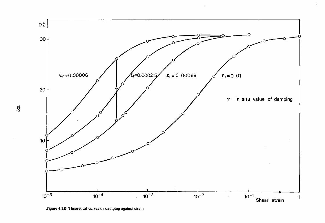
I I I 10~ 5 10" 4 10" 3
Figure 4.2D Theoretical curves of damping against strain
E r = 0 . 0 0 0 6 8 O £ r =0.01
v In si tu v a l u e of damping
10 - 2 10" 1
Shear strain
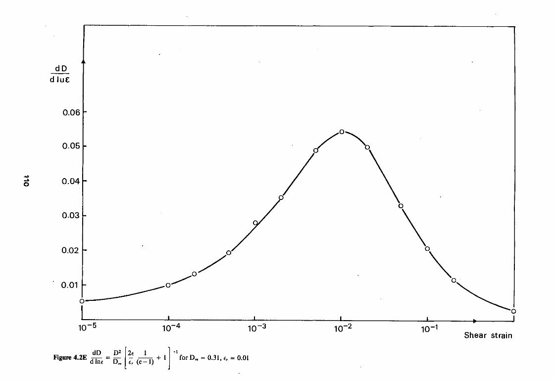
d D
d l u £
0.06
0.05
0.04
0.03
0.02
0.01
10 - 5 10 - 4 10 -3
Figure 4.2E dD _ D 2
dine ~ Dl 2e 1 r (FT)
+ 1 -1 for D m = 0.31, er = 0.01
10 -2 10 - 1
Shear strain

4.2.3 Calculation of radius of curvature
A positive value of the damping implies curvature of the stress strain
dependence. The area of the hysteresis loop AE in equation 4.5 is
positive as shown in figure 4.2F. The radius of curvature R may be
calculated from the shear modulus G at small strain and a value of Q
corresponding to a known strain e, from this figure
Half area of loop = | R2 - R2sin y cos
area of loop AE = R2(<{>- sin <j>) the energy lost per cycle
E = i e2 cot 9 the energy stored per cycle.
T . 1 AE R2(<j> - sin <J>) Loss factor — = n _ = — — — X ¥EZ cot 9
Now R sin I- = .g . R = 4.19 2 sin 9
4> sin 9 sin -J
_1_ = (<{> - sin <j>) _ 2 (<{> - sin <j>) Q
¥ cot 9 sin2e sin2 ¥ sin 29 sin2
<(> is the solution to
s l n 2 ! - r i s - s e - s i n •> 4- 2 0
111
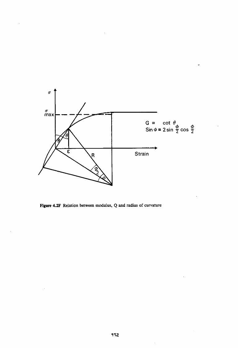
112

CHAPTER 5
SOME EXAMPLES OF THE MEASUREMENT OF IN SITU DAMPING
5.1 In situ methods
The previous chapter has shown that the modulus of a viscoelastic material
can change considerably with time and that this dependence is proportional
to the damping factor at the appropriate level of strain, to a first
approximation. This damping factor may increase with strain up to some
64%. Such behaviour varies with the material and so it becomes very
important to measure the damping factor at a known level of strain for
the material in question. This chapter describes some of the methods that
have been applied to measurements in the field, where effects of sampling
have been reduced to a minimum.
5.1.1 Hammer damping
One of the easiest ways of obtaining a measure of the Q of a material is
to strike it with a hammer and observe the decay of the resultant
vibrations, see figure 4.ID. This may be done with a hammer seismograph
such as the Bison or Nimbus, section 2.1 and figures 2.IE and 2.IF, and
photographs taken of the resulting decay curve. From measurements of the
amplitudes, the logarithmic decrement 5 may be found from equation 4.6 and
Q from equation 4.7.
Several observations were made with the hammer seismograph at the site on
the London clay at Brent Cross where plate tests (Marsland, 1971) and
pile tests (Cooke and Price, 1973) have been completed. Some measurements
* A useful rule of thumb is to count the number of positive peaks that can be seen; this number is then approximately equal to the Q of the material.
HFDAAI 113

were also made on the Boulder clay at the Building Research Station North
Field site.
Eight small chambers 0.3 m x 0.3 m x 0.3 m, were cut in the side of an
excavation in the London clay at Brent. They were on three levels, 0.8,
1.05 and 1.35 m below the surface. On the base of the chambers a 140 mm
diameter plate was set in plaster of Paris. The plate was struck
vertically by a small hammer fitted with an inertia switch to trigger the
seismograph (see figure 5.1A). A decay photograph as shown in figure 5.IB
was taken with a Polaroid camera. The logarithmic decrements were found
from 17 measurements. The average value of Q was 2.3 ± 0.7, corresponding
to a strain estimated at about 0.1%.
As there could be energy lost by radiation even if the material were
perfectly elastic, the fraction of energy lost in that way was estimated
at about 15% on the basis of the equations given by Miller and Pursey
(1955). They give the total power W radiated by a disc source vibrating
on the edge of a semi infinite elastic half space as
4.836 ir3 f2 r4 P 2 W = 5.1
pVc3
where r is the plate radius, P Q the maximum pressure exerted, and Vc the
compression wave velocity. P Q may be estimated from the punch equation
e = I r (l-v2) 5.2
by calculating the elastic energy stored due to the displacement.
This correction was subtracted from the measured value of 1/Q to find
the true value corresponding to the energy lost within the material.
114
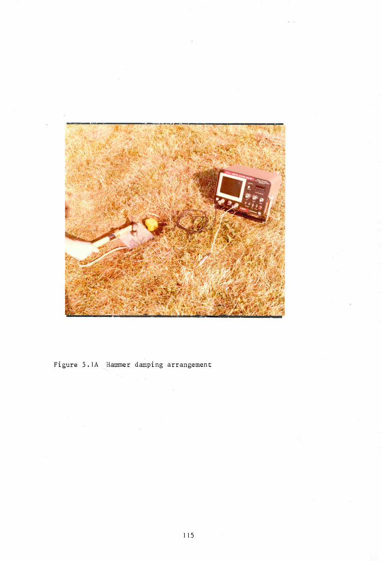
Figure 5.1A Hammer damping arrangement
1 15

Figure 5.IB Hammer damping
1 16
5.1.2 Plate resonance
A plate resting on the surface of the ground or on the base of one of the
chambers and vibrated vertically is equivalent to a damped spring mass
system to a first approximation. The resonance is similar to that shown
in figure 4.IE and the bandwidth of this resonance can be used to measure
the damping. This technique was also used at Brent Cross.
A Ling model 101 vibrator was screwed to the centre of the 140 mm diameter
plate, described previously, and fed from an ITT audio amplifier receiving
a signal from a tuneable oscillator. The resulting vibration was detected
by a Sensor SM2 geophone placed next door to the plate, the voltage being
read by a Levell wideband voltmeter. Usually a resonance peak was found
in the region of 250 Hz as shown in figure 5.1C. The Q was found from the
bandwidth at the 0.707 peak amplitude points from equation 4.7.
From 14 such curves, the mean value of Q was 2.9 ± 0.7. Some curves, not
used to calculate Q, showed double peaks and this was thought to be due to
the effects of local fissuring. One chamber had been flooded for some
weeks and gave very low resonance peaks. The strains involved are thought
to be smaller than for the hammer damping experiment and in the region of
2 x 10~2%. This was estimated from the amplitude of the vibration and
also from the measured amount of power delivered by the amplifier. A
voltage was measured across a one ohm resistance in series with the
vibrator. The fraction of energy then lost by radiation was estimated at
about 5%.
The values of damping obtained from hammer damping and plate resonance
tests are above the reported values for saturated clays (Bolton Seed and
117
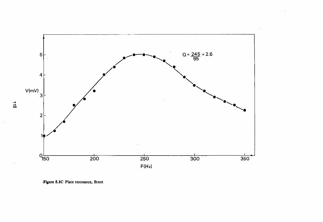
V(mV)
150 200 250 F(Hz)
•Figure S.1C Plate resonance, Brent
Q = 245 =2.6 95
300 350
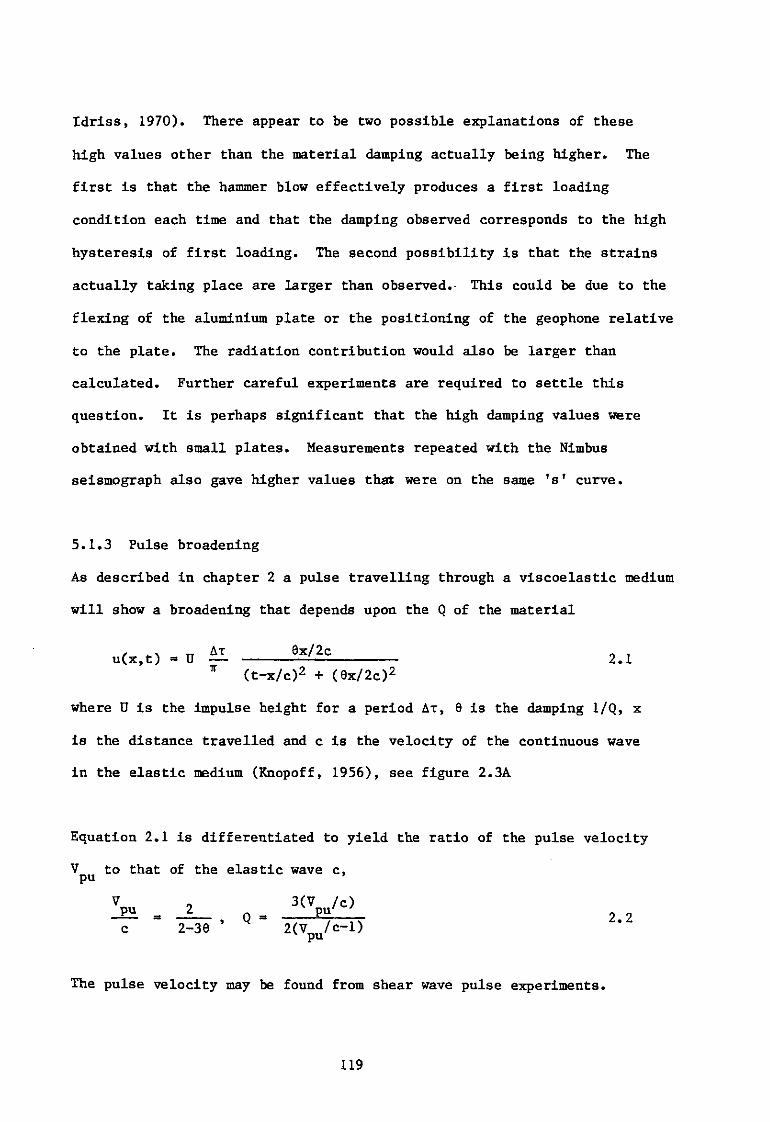
Idriss, 1970). There appear to be two possible explanations of these
high values other than the material damping actually being higher. The
first is that the hammer blow effectively produces a first loading
condition each time and that the damping observed corresponds to the high
hysteresis of first loading. The second possibility is that the strains
actually taking place are larger than observed. This could be due to the
flexing of the aluminium plate or the positioning of the geophone relative
to the plate. The radiation contribution would also be larger than
calculated. Further careful experiments are required to settle this
question. It is perhaps significant that the high damping values were
obtained with small plates. Measurements repeated with the Nimbus
seismograph also gave higher values that were on the same 's' curve.
5.1.3 Pulse broadening
As described in chapter 2 a pulse travelling through a viscoelastic medium
will show a broadening that depends upon the Q of the material
F RR AT 8X/2C « . u(x,t) = U — 2.1 * (t-x/c)2 + (0x/2c)2
where U is the impulse height for a period AT, 9 is the damping 1/Q, x
is the distance travelled and c is the velocity of the continuous wave
in the elastic medium (Knopoff, 1956), see figure 2.3A
Equation 2.1 is differentiated to yield the ratio of the pulse velocity
V to that of the elastic wave c, pu ' V 0 3(V / c) JB2. = n = P u 2 2 c 2-36 ' " 2(Vpu/c-1)
The pulse velocity may be found from shear wave pulse experiments.
119
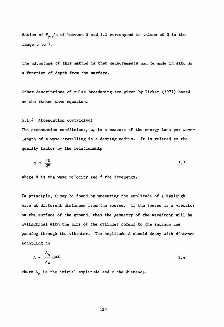
Ratios of V /c of between 2 and 1.3 correspond to values of Q in the
range 3 to 7.
The advantage of this method is that measurements can be made in situ as
a function of depth from the surface.
Other descriptions of pulse broadening are given by Ricker (1977) based
on the Stokes wave equation.
5.1.4 Attenuation coefficient
The attenuation coefficient, a, is a measure of the energy loss per wave-
length of a wave travelling in a damping medium. It is related to the
quality factor by the relationship
irf _ 0 a = w 5- 3
where V is the wave velocity and f the frequency.
In principle, Q may be found by measuring the amplitude of a Rayleigh
wave at different distances from the source. If the source is a vibrator
on the surface of the ground, then the geometry of the wavefront will be
cylindrical with the axis of the cylinder normal to the surface and
passing through the vibrator. The amplitude A should decay with distance
according to
A A = — e ^ 5.4
/x
where Aq is the initial amplitude and x the distance.
120
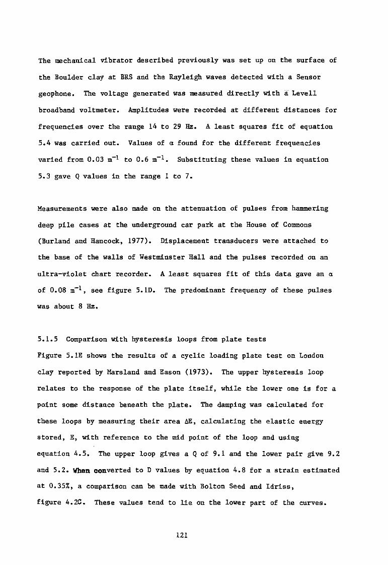
The mechanical vibrator described previously was set up on the surface of
the Boulder clay at BRS and the Rayleigh waves detected with a Sensor
geophone. The voltage generated was measured directly with a Levell
broadband voltmeter. Amplitudes were recorded at different distances for
frequencies over the range 14 to 29 Hz. A least squares fit of equation
5.4 was carried out. Values of a found for the different frequencies
varied from 0.03 m"1 to 0.6 m"1. Substituting these values in equation
5.3 gave Q values in the range 1 to 7.
Measurements were also made on the attenuation of pulses from hammering
deep pile cases at the underground car park at the House of Commons
(Burland and Hancock, 1977). Displacement transducers were attached to
the base of the walls of Westminster Hall and the pulses recorded on an
ultra-violet chart recorder. A least squares fit of this data gave an a
of 0.08 m-1, see figure 5.ID. The predominant frequency of these pulses
was about 8 Hz.
5.1.5 Comparison with hysteresis loops from plate tests
Figure 5.IE shows the results of a cyclic loading plate test on London
clay reported by Marsland and Eason (1973). The upper hysteresis loop
relates to the response of the plate itself, while the lower one is for a
point some distance beneath the plate. The damping was calculated for
these loops by measuring their area AE, calculating the elastic energy
stored, E, with reference to the mid point of the loop and using
equation 4.5. The upper loop gives a Q of 9.1 and the lower pair give 9.2
and 5.2. When converted to D values by equation 4.8 for a strain estimated
at 0.35%, a comparison can be made with Bolton Seed and Idriss,
figure 4.2C. These values tend to lie on the lower part of the curves.
121

I I , o 10 20 30
x(m)
Figure S.lD Accelerations measured at Westminster
I ,. 40 50
122
I
60
a Il ms - 2
- x10-1
- x10-2
- x10-3

4.5 L o a d - U n l o a d Reload-Unload
Loading plate
mm
beneath loading plate
100 200 300 400 500 600 Bearing pressure (KN/m 2 )
700 800
Figure 5.1E Plate tests at Brent Cross
123

5.2 Damping factor (1/Q) as a function of strain
The damping factor 1/Q has been measured as a function of strain for clays
and sands (Bolton Seed and Idriss 1970). The results for clays are
summarised in figures 4.2A and 4.2C and as can be seen they form an 's'
shaped curve. In figure 4.2A the average curve of D has values between 3%
at 10~5 shear strain and 28% at 10""1 strain. The upper and lower curves
shown are the bounds of several sets of experimental data from a variety
of clay samples. Average values appropriate to the strain involved were
used to calculate moduli from geophysical data to compare with plate tests
and pressuremeter measurements (Abbiss 1981 ). The upper and lower
bounds of figure 4.2C fitted to in situ data were used to calculate the
uncertainty due to the contribution from damping, for the North Field
settlement calculations.
Recent large scale in situ measurements of 1/Q have been made by
cyclically loading a 0.457 m dia pile 9.1 m long in glacial till at
Gowden (Gallagher, 1980). Plots of stress against strain, figure 5.2A,
for different amplitudes show hysteresis loops that enable the damping
factor to be found at different strains from equation 4.5.
The results are plotted as triangles in figure 4.2C and are close to the
average curve for strains of 8 x 10""5 to 6 x 10""1*. The shear strains
were estimated by assuming that the strain around the pile extended for
approximately 3 pile diameters (Cooke and Price, 1973).
5.3 Measurement of Q by autocorrelation of seismic noise
An interesting possibility is that the autocorrelation function of a
filtered seismic noise signal may yield the damping properties of the
124

0 . 4 5 7 m dia 9 . 1 2 4 m length Glacial till (Cowden upper)
Pile displacement (mm)
Figure S.2A Hysteresis loops
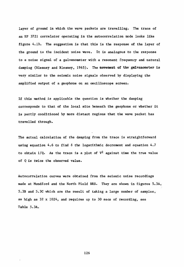
layer of ground in which the wave packets are travelling. The trace of
an HP 3721 correlator operating in the autocorrelation mode looks like
figure 4.ID. The suggestion is that this is the response of. the layer of
the ground to the incident noise wave. It is analogous to the response
to a noise signal of a galvanometer with a resonant frequency and natural
damping (Bleaney and Bleaney, 1965). The movement of the galvanometer is
very similar to the seismic noise signals observed by displaying the
amplified output of a geophone on an oscilloscope screen.
If this method is applicable the question is whether the damping
corresponds to that of the local site beneath the geophone or whether it
is partly conditioned by more distant regions that the wave packet has
travelled through.
The actual calculation of the damping from the trace is straightforward
using equation 4.6 to find 6 the logarithmic decrement and equation 4.7
to obtain 1/Q. As the trace is a plot of V2 against time the true value
of Q Is twice the observed value.
Autocorrelation curves were obtained from the seismic noise recordings
made at Mundford and the North Field BRS. They are shown In figures 5.3A,
5.3B and 5.3C which are the result of taking a large number of samples,
as high as 32 x 1024, and requires up to 30 sees of recording, see
Table 5.3A.
126
0.3 V2
r\j "N3
0
Figure 5.3A Autocorrelation for chalk, Mundford
33ms
Figure 5.3B Autocorrelation for boulder clay, North Field
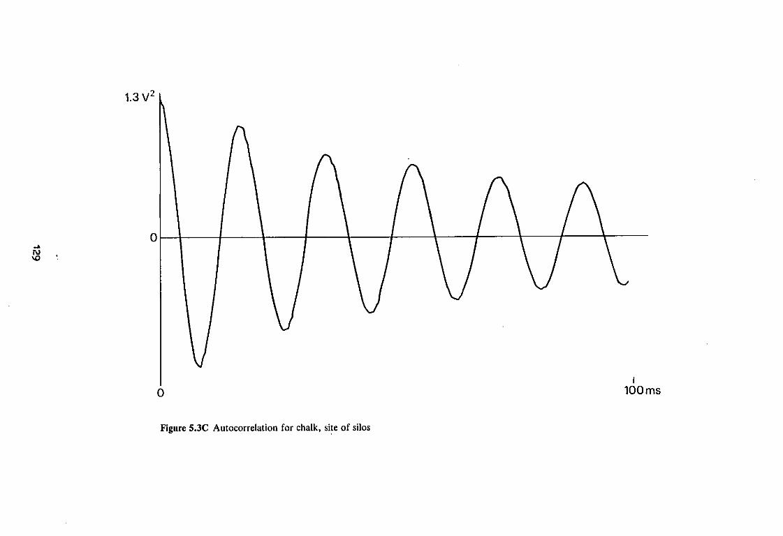
Figure 5.3C Autocorrelation for chalk, site of silos

TABLE 5.3A Q FROM AUTOCORRELATION
Q Average strain D% f (Hz) \(m)
N Field (dry) 1 11 3 . 0 X 10" 9 4 . 4 30 5 2 1 . 4 . 8 2 2 14 2 . 5 X 10~9 3 . 6
3 30 2 . 1 X 10- 9 1.7 4 38 1 .8 X 10" 9 1 .3
N Field (wet) 1 9 . 9 3 .7 X 1 0 - 9 5 . 0 30 5 1 0 . 8 . 8 1 2 11. 3 2 . 8 X 10- 9 4 . 5
3 13. 4 2 . 2 X 10" 9 3 .7 4 44 1 . 8 X 10- 9 1 .1
Site of silos 1 26 9 . 1 X lO"9 1 .9 4 . 8 . 8 1 2 21 7 . 9 X 10" 9 2 . 3 10 .6 26
3 40 7 . 1 X 10" 9 1 .2 4 34 6 . 5 X 1 0 - 9 1 .5 5 49 6 . 0 X lO"9 1 .0
Mundford 1 99 1 .7 X 1 0 " 1 0 0 . 5 30 33 2 94 1.7 X 1 0 " 1 0 0 . 5 3 182 1 .7 X 1 0 - i o 0 . 3 4 86 1 .6 X 1 0 - i o 0 . 6
HFDAAJ 130
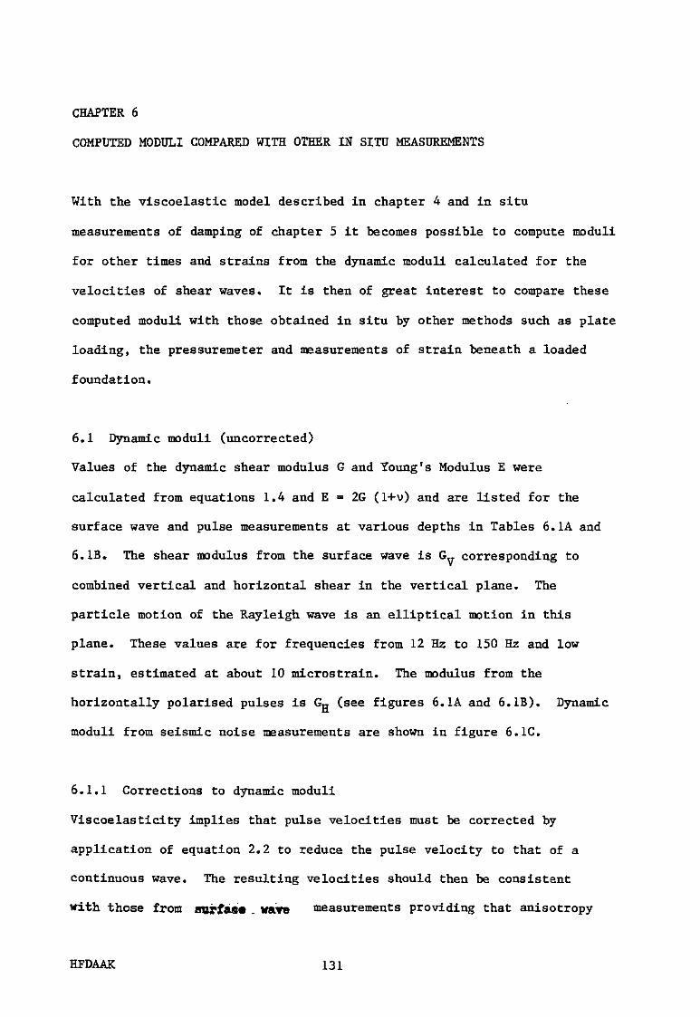
CHAPTER 6
COMPUTED MODULI COMPARED WITH OTHER IN SITU MEASUREMENTS
With the viscoelastic model described in chapter 4 and in situ
measurements of damping of chapter 5 it becomes possible to compute moduli
for other times and strains from the dynamic moduli calculated for the
velocities of shear waves. It is then of great interest to compare these
computed moduli with those obtained in situ by other methods such as plate
loading, the pressuremeter and measurements of strain beneath a loaded
foundation.
6.1 Dynamic moduli (uncorrected)
Values of the dynamic shear modulus G and Young's Modulus E were
calculated from equations 1.4 and E = 2G (1+v) and are listed for the
surface wave and pulse measurements at various depths in Tables 6.1A and
6.IB. The shear modulus from the surface wave is Gy corresponding to
combined vertical and horizontal shear in the vertical plane. The
particle motion of the Rayleigh wave is an elliptical motion in this
plane. These values are for frequencies from 12 Hz to 150 Hz and low
strain, estimated at about 10 microstrain. The modulus from the
horizontally polarised pulses is G^ (see figures 6.1A and 6.IB). Dynamic
moduli from seismic noise measurements are shown in figure 6.1C.
6.1.1 Corrections to dynamic moduli
Viscoelasticity implies that pulse velocities must be corrected by
application of equation 2.2 to reduce the pulse velocity to that of a
continuous wave. The resulting velocities should then be consistent
with those from surf&ea_wave measurements providing that anisotropy
HFDAAK 131
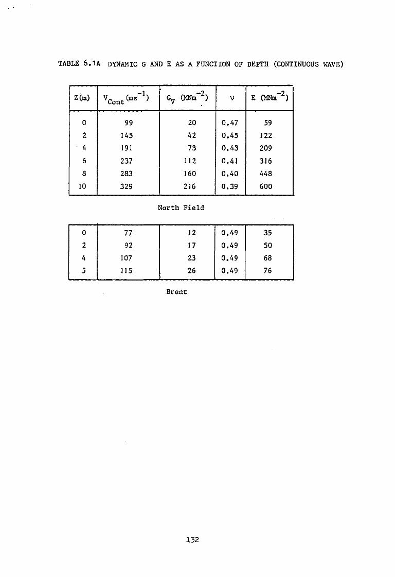
TABLE 6.1 A DYNAMIC G AND E AS A FUNCTION OF DEPTH (CONTINUOUS WAVE)
Z(m) VCont ( m r l ) Gy (MNnf2) V E (MNm"2)
0 99 20 0 .47 59
2 145 42 0 . 4 5 122
• 4 191 73 0 . 4 3 209
6 237 112 0 .41 316
8 283 160 0 . 4 0 448
10 329 216 0 . 3 9 600
North Field
0 77 12 0 . 4 9 35
2 92 17 0 . 4 9 50
4 107 23 0 . 4 9 68
5 115 26 0 . 4 9 76
Brent
132
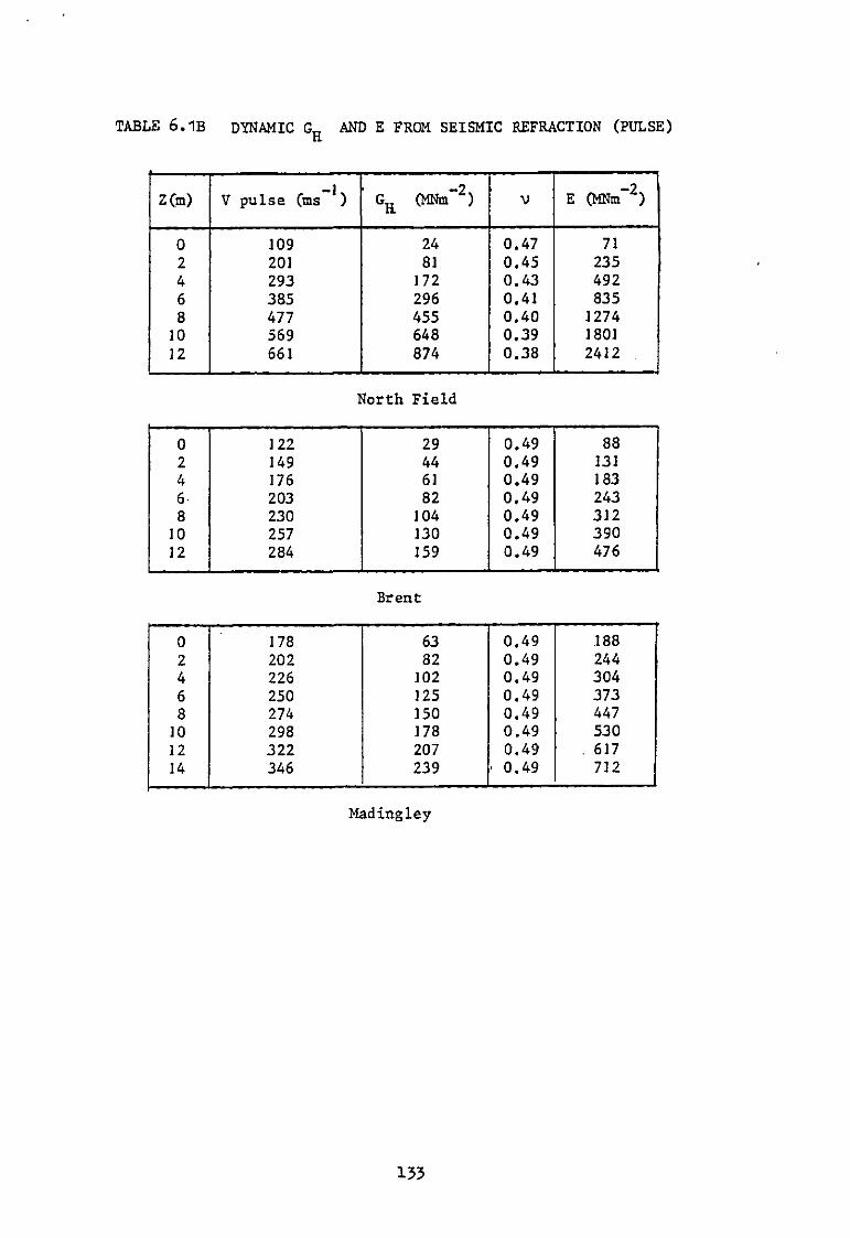
TABLE 6.1B DYNAMIC G„ AND E FROM SEISMIC REFRACTION (PULSE)
ZCm) V pulse (ms *) G R (MNm~2) V E CMNm"2)
0 109 24 0.47 71 2 201 81 0.45 235 4 293 172 0.43 492 6 385 296 0.41 835 8 477 455 0.40 1274 10 569 648 0.39 1801 12 661 874 0.38 2412
North Field
0 122 29 0.49 88 2 149 44 0.49 131 4 176 61 0.49 183 6- 203 82 0.49 243 8 230 104 0.49 312 10 257 130 0.49 390 12 284 159 0.49 476
Brent
0 178 63 0.49 .188 2 202 82 0.49 244 4 226 102 0.49 304 6 250 125 0.49 373 8 274 150 0.49 447 10 298 178 0.49 530 12 322 207 0.49 . 617 14 346 239 • 0.49 712
Madingley
133

G,MNm~2
Figure 6.1A Shear moduli G, Brent (low strain)

G, MNrri2
Figure 6.1B Shear moduli G, North Field (BRS)
135

200 300 GMNm - 2
o Bricket Wood, Boulder clay v Brent, London clay A Christchurch bay • 865mm dia plate tests
corrected to low strain level (Brent)
Z(m)
Figure 6.1C Dynamic shear moduli against depth, swimming pool, Brent, and Christchurch bay, compared with static moduli at Brent
136

is taken into account. The dynamic modulus calculated from these
velocities by equation 1.4 then corresponds to the period Ti of the wave
in question.
The dynamic modulus must be corrected to obtain the static modulus for
the required time T2 by equation 4.16 using a value of Q that corresponds
to the strain produced. A simple calculator program has been written so
that the calculation may be undertaken in the field.
6.2 Comparison with other measurements
The 'static' moduli for time T2, and the appropriate strain, found from
the dynamic values are compared with those obtained by plate test and
pressuremeter.
6.2.1 Comparison with plate tests at Brent
At Brent the measurements are compared with values for London clay
obtained from large scale plate tests (Marsland, 1971) see figure 6.2A
and Table 6.2A. These plate tests took an average time of about 0.6
minutes and were at an average strain of 2 x 10~1%. The dynamic values
from the shear wave refraction survey are corrected to these levels of
time and strain.
For this site in situ determinations of damping, sections 5.1.1 and 5.1.2
had been made by hammer damping and plate resonance. As discussed these
values lay above the curves of Bolton Seed and Idriss. On the other hand
hysteresis measurements from the 865 Tnm plate tests themselves, section
5.1.5 lay in the lower half of the range of their curves, see figure 4.2C.
It was felt that the damping values from the plate tests would correspond
137

0 , 10 4 Q i I
G,MNrrf2
30 40 50 T
60 T
70 80
• Plate tests 0 Calculated from seismic velocities
1 1 Error due to uncertainty in Q I 1 Error due to uncertainty in Gdyn
Average time 0.6mins Average strain 2x10~1%
Figure 6.2A Comparison with plate tests at Brent
138

TABLE 6.2A COMPARISON WITH PLATE TESTS AT BRENT
z (m)
Seismic MNm"2
GDyn MNm"2
Sin MNm"2
Sean MNm"2
S a x MNm"2
0 29 21 6 7 12
2 44 32 5 11 19
4 61 44 7 15 26
6 82 59 10 20 34
8 104 75 12 26 44
10 130 94 15 32 55
12 159 115 19 39 67
G,, was found for e ~ 10"3%, D Dyn Plate tests were carried out at and average strain of 2 x 10_1%
0 = 4.2, 0 . = 2.5 Tnean inin
<-5%, Q = 10
an average time of 0.6 minutes for which Q ^ ^ =8.3,
TABLE 6.2B COMPARISON WITH WINDLE AND WROTH. Q VALUES FROM FIG 4.2A (BOLTON SEED AND IDRISS 1970)
Z(m) Av. strain % Sin Sean Sax S i n G mean G max
2 1.2 x 10"1 2.9 5.6 12.5 7.5 20 37
4 0.65 x 10"1 3.8 6.3 16.7 15 29 52
6 0.33 x 10"1 5.0 8.3 25.0 27 44 71
139
most closely to the viscoelastic properties required to make the
correction. On this basis the range of values of G calculated from the
seismic measurements is the upper half of the range shown in figure 6.2A,
using the procedure outlined in section 6.1.1. The total range is from
the data of Bolton Seed and Idriss.
It should be pointed out that these plate test values are for reloading.
Initial loading produced lower stiffnesses, while corrections to lower
levels of strain would double the stiffness (Marsland and Eason, 1973).
Thus in this case a value of damping measured at known strain was used to
determine the appropriate 's' shaped curve of damping factor against
strain, ie to determine e^. This damping curve was then used to correct
the moduli to the required times and strains.
6.2.2 Comparison with pressuremeter at Madingley
At Madingley, Cambridge, the material Is the Gault clay and the results
are compared with pressuremeter measurements, (Windle, 1976) figure 6.2B,
Table 6.2B and the PIP or push in pressuremeter results (Henderson et al,
1979) figure 6.2C, Table 6.2C. These were at relatively high strain
values of up to 1.5%. The times of measurement varied from 2 to 24
minutes.
As described in section 2.1.3 a shear wave refraction survey was carried
out on this site. The corrected values of G are listed in Tables 6.2B
and 6.2C. These corrections were made using the damping curves of
Bolton Seed and Idriss. It would have been preferable to use a damping
curve determined by an in situ measurement of damping at known strain.
140

0
2 -
Z(m) 5 -
7 -
8
10
10 20 30 -T~~
G,MNm 40
-2
50 60 70 80
Windle and Wroth A Rate cr 6mins • Rate 13 12mins • Rate 7 24 mins
o Seismic, calculated for same strain levels and an average time of 6 minutes
Error due to uncertainty in Q I 1 Error due to uncertainty in Gd y n
Figure 6.2B Comparison with Windle and Wroth, Madingley, Cambridge
141

G,MNrri2
Figure 6.2C Comparison with pressure-meter measurements, Cambridge 142
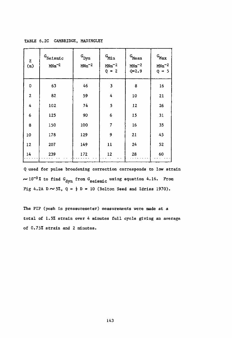
TABLE 6.2C CAMBRIDGE, MADINGLEY
z Seismic GDyn Sin Sean S a x (m) MNm"2 MNm"2 MNm"2 MNm"2 MNm"2
Q = 2 Q=2.9 Q = 5
0 63 46 3 8 16
2 82 59 4 10 21
4 102 74 5 12 26
6 125 90 6 15 31
8 150 100 7 16 35
10 178 129 9 21 45
12 207 149 11 24 52
14 239 172 12 28 60
Q used for pulse broadening correction corresponds to low strain
to find G j ^ from ^ s ei s m£ C using equation 4.16. From
Fig 4.2A D~>5%, Q = \ D - 10 (Bolton Seed and Idriss 1970).
The PIP (push in pressuremeter) measurements were made at a
total of 1.5% strain over 4 minutes full cycle giving an average
of 0.75% strain and 2 minutes.
143

This awaits the development of a satisfactory method of measuring
damping in situ.
In an earlier paper (Morris and Abbiss, 1979) comparisons were made by
means of the strain correction of Hardin and Drnevich (1972) but this
did not account for the time dependence, which required the use of the
viscoelastic theory.
6.2.3 Comparison with in situ values at Mundford
Shear wave measurements were made by refraction survey as described in
section 2.1.5. These were confirmed by seismic noise measurements see
this survey are listed in Tables 6.2D, E. The value of Poisson's ratio
used was 0.24 as this was found from laboratory tests, In situ tests and
spanned by the dynamic values obtained using the p-wave velocities.
The factor 0.47 in E g t = 0.47 was the same as used in the paper which
compared stiffnesses from the p-wave survey with those determined by
computer back analysis and plate tests (Abbiss, 1979).
Further evidence for this factor was obtained by measurements on a
specimen of chalk in the laboratory both by resonance methods and the
decay of a hammer blow. The mean value of Q found was 17. For linear
behaviour equations 4.16 and 2.2 may be combined
figure 2.1M. The Poisson's ratio moduli G and E static from
6.1
144

TABLE 6.2D POISSON'S RATIO, MUNDFORD
Depth Z (m) V (ms"1) s V (ms"1) P V
0 590 374 not valid 5 680 874 -0.27 10 770 1374 0.27 15 860 1874 0.37 20 950 2374 0.40
0.5(V/Vg)2-1 f r o m v " — ( V /V )2-l p s
TABLE 6.2E MODULI, RELATIVE TO DEPTH BELOW TANK D, MUNDFORD
D G, MNm"2 dyn Edyn(v = 0.24) E = 0.47 E st dyn
0 769 1907 896 5 1008 2500 1175 10 1288 3194 1501 15 1585 3931 1847 20 1922 4766 2240
G, = 769 + 57.7z dyn o/v i I 7 9 x 9.15 x 1.0 8/b = 1.46, w =» = 1.1 mm 2 x 769
Central settlement w . = 2.3 mm st cf 2.6 observed
w u s l n g w3t = orfr
145

For Ti = 0.01 sees and T2 • 105 sees
Est = 0.55 X 0.83 = 0.46 ± 0.1 dyn
The corresponding creep rate for the chalk is 9% per cycle which is close
to the reported values of between 10 and 15% (Burland and Lord, 1969).
These values for chalk are assumed to correspond to fairly low strains.
E is plotted as a function of depth in figure 6.2D where it is compared
with the values shown by the dotted line from back analysis using finite
elements (Burland, Sills and Gibson, 1973) and plate tests (Burland and
Lord, 1969). The agreement is better near the surface and suggests that
the quality factor may increase with depth, ie in the deeper rock chalk
there may be a smaller difference between E . and E, J st dyn
6.3 Accuracy
The error or standard deviation in the dynamic shear modulus is made up
from the error in shear velocity AV and the error in density Ap from
equation
AG = Ap + 2AV 6.2
(a) Shear wave refraction
For the North Field AV increased from 7% at 5 m to 14% at 11 m. A full
survey of densities was not carried out so Ap is not known. Thus the
error in G is a minimum estimate and varies from 14% to 28%.
At Brent AV was 8% at 3 m, 2% at 6 m and 4% at 9 m. A full survey of
densities had been carried out (Marsland, 1977) and the standard deviation
146

1000 2000 3000 4 0 0 0 5000 EMNm - 2
Seismic From finite element
• Plate test
Figure 6.2D Comparison with plate tests and finite elements, Mundford 147

was 2%. This gives a combined error of 18%, 6% and 10%. The uniformity
of the density on this site was confirmed by a very constant plot of back
scattered y radiation from a borehole log.
At Madingley the pattern of errors was thought to be similar to that
obtained at the North Field site. Values of the density of the Gault
clay were taken from a survey carried out for the Ely-Ouse tunnel
(Samuels, 1975). They were again very consistent and the value of Ap
was 3% so that AG was estimated at from 17% to 31%.
(b) Surface wave
For the North Field the standard error in the velocity is ± 15 ms"1 and
the combined error in G . is a minimum of 20%.
The standard error of the velocity from a linear plot at Brent is 3 ms"1.
Combined with Ap this gives an average standard error for Gv of 9%.
148
CHAPTER 7
CALCULATION OF SETTLEMENT
7.1 Methods of calculation
Settlements have been calculated using finite element programs for ground
where the modulus increases with depth. (Burland and Lord, 1969 and
Burland and Wroth, 1974). Also the cases of circular and rectangular
areas on a half space whose stiffness increases linearly with depth have
been solved analytically. (Brown and Gibson, 1972 and 1979). If the
variation of G with depth is given by
G = G(o) + mz 7.1
the first of the analytical papers presents graphs of the central
settlement x 2G(o)/qb where q is the loading pressure and b is the radius
of the circular area, as a function of G(o)/mb for different values of
Poisson's ratio v. The second paper gives families of curves of
wE/qB(l-v2) where w is the corner settlement as a function of L/B, E is
the Young's Modulus, B the breadth and L the length. The curves are
plotted for different values of 3/d and B/d where 3 = G(o)/m and d is
the depth to a rigid base.
The geophysical measurements give G(o), m, v and E for short times.
B and q are known so w may be found for short times by interpolation
between the appropriate curves.
The corresponding value of strain may be estimated for the known 3 from
the surface profile curves given in the first paper for values of L/B
not too far from unity.
HFDAAL 149

The damping factor (1/Q) for this level of strain may now be read off from
figure 4.2D and the variation of effective modulus with time found from
equation 4.16. As a first approximation w is assumed to be inversely
proportional to G(T) for up to three or four orders of magnitude in
time
The generalised viscoelastic solid is usually assumed to have (1/Q)
varying slowly with time. This may be expressed by saying that the
damping factor is effectively constant in time. However it has been
suggested that it must eventually drop to zero at very long times
(Lomnitz, 1974 and Pliant, 1979).
7.2 1 m square pads in North Field BRS
A test that corresponded as closely as possible to the ideal theoretical
model was carried out in the North Field at the Building Research Station.
Square concrete pads 1 m x 1 m were cast on the Boulder clay at depths of
1.0 m and 0.33 m, the first pad being at the base of a 1 m deep pit. Each
pad was loaded by crane with five sections of steel kentledge weighing
approximately 2 tonnes each, see figures 7.2A and 7.2B. Thus the pressure
under each pad could be raised to 109.5 kNm-2 in about 20 minutes, the
time taken for the loading operation.
Each pad was fitted with studs as levelling points and the level measured
relative to a deep datum some 10 m away by means of an invar staff and
Wild NA2 automatic level (Cheney, 1973). Readings were taken before and
7.2
150

Figure 7.2A 1 m square pad, 1.0 m depth, North Field
Figure 7.2B 1 m square pad, 0.3 m depth, North Field
151
immediately after the loading was completed, and then at subsequent times
to produce the observations of settlement shown in figures 7.2C, D, F, G.
The theoretical settlement curves were calculated from the dynamic moduli
in two stages. The first stage shown in figures 7.2C and 7.2D was from
the viscoelastic model as in 7.1 with the damping factor falling to one
half of its dynamic value by the time of one hour. There was some
justification for this in terms of the drainage paths under the pads.
Because the pads were effectively rigid the settlement has been found
using the approximation
w . ., = 1/3 (2w . + w ... 7.3 rigid centre corner flexible from Davis and Taylor (1962) with w . 2 w from the settlement J centre corner profiles shown in Brown and Gibson (1972).
The main sources of error appear to be the spread of possible values of
(1/Q) and the difficulties of interpolation for v, 8/d and B/d. Care has
to be taken with the linear fit of G(z) to ensure that the values near the
surface are correct even if the fit is not quite so good for some of the
deeper values, ie G(o) must be correct.
The variation of shear modulus as a function of strain after one hour is
of interest and is tabulated in Table 7.2A. This is based on equation
4.16 with 1/Q varying with strain according to the s-shaped curve given
in figure 4.2D with er = 0.00021 corresponding to the fit of in situ
damping for the North Field. The graph of G against e is plotted in
figure 7.2E.
152
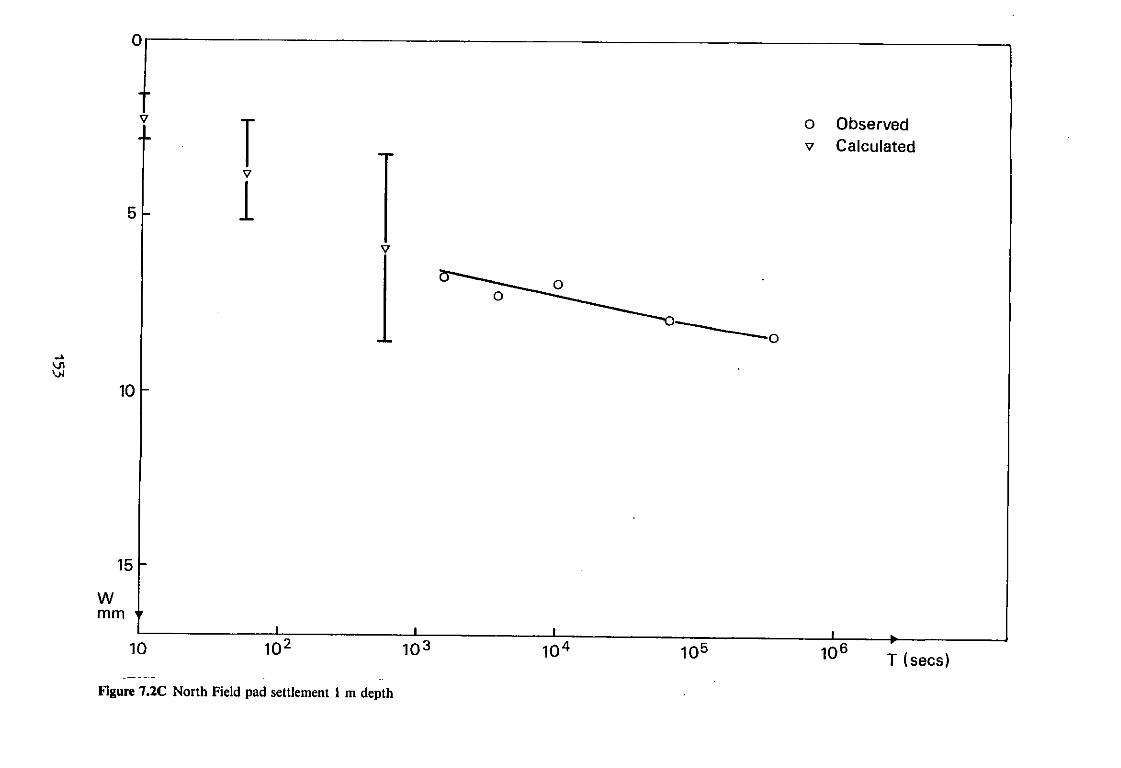
0
10
I v 1
15
W mm
10 10 103
Figure 7.2C North Field pad settlement 1 m depth
Observed Calculated
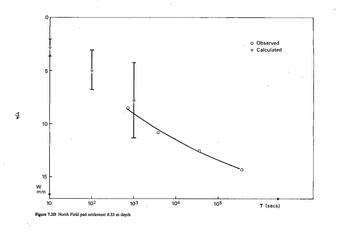
0
\J1 -p-
10
v 1
15
W mm
10 102 1 0 3
Figure 7.2D North Field pad settlement 0.33 m depth
o Observed v Calculated
T (sees)
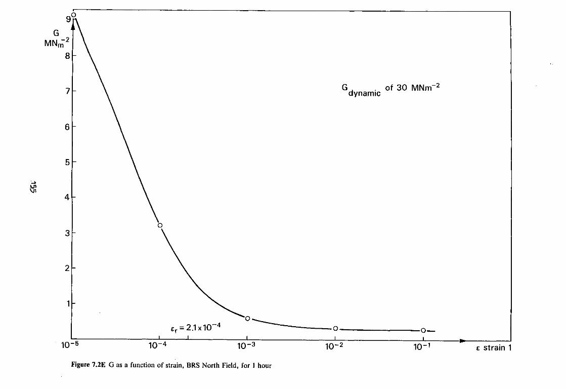
.yi
IO-5 1 0 " 4 1 0 " 3
Figure 7.2E G as a function of strain, BRS North Field, for 1 hour
G , . of 30 MNm"2
dynamic
•o— _i
10-2 10"1 E strain 1

7.2.1 Three dimensional consolidation
Beyond a time of one hour the second stage of the settlement was
calculated from three dimensional consolidation theory (Davis and Poulos,
1968). The curves are shown in figures 7.2F and 7.2G. These are based on
an in situ value of the permeability of 10~7 ms"1 measured by means of a
falling head of water with a stand pipe and piezometer head.
The time factor Ty. used in these calculations was given by
°v3 t T v = —
where t is time, c ^ Ls the three dimensional coefficient of consolidation
and h is the depth of the permeable layer.
k E' c = 7.2
3yw (1-2V)
with k the coefficient of permeability, E1 the effective stress Young's
modulus and v' the effective stress Poisson's ratio.
E' = 2G'(1+v') 7.3
The values of consolidation ratio Up are tabulated against time in Table
7.2B and were found from graphs given by Davis and Poulos (1968). The
settlements of the pads are wi and W£ respectively, shown in figures 7.2F
and 7.2G.
These settlements are for the initial loading of the clay and correlate
with the high damping values of figure 4.2D. Reloading settlements would
probably be smaller and correspond to smaller values of damping.
156
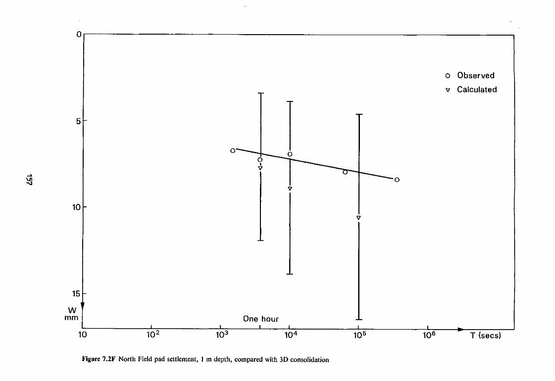
Figure 7.2F North Field pad settlement, 1 m depth, compared with 3D consolidation

Figure 7.2G North Field pad settlement, 0.3 m depth, compared with 3D consolidation

TABLE 7.2A G AS A FUNCTION OF STRAIN AFTER 1 HOUR
Strain e D% 1/Q G(1 hr) MNm"2
10"5 8 0.16 9.1 10"4 15 0.30 3.2 10"3 26.5 0.53 0.58 lO-2 30.5 0.61 0.32 10"1 31 0.62 0.30
TABLE 7.2B SETTLEMENT FROM CONSOLIDATION
t(secs) T V Up wi (mm) W2(mm)
3.6 x 10³ 5.9 x 10"4 0.66 7.7 9.6
104 1.6 x 10"3 0.76 8.9 11.1
105 1.6 x 10"2 0.91 10.6 13.2
00 1.0 11.7 14.6
7.3 Large silos founded on chalk
Shear wave velocities were measured at the site of four large silos each
capable of holding 12 000 tonnes and standing some 50 m high, see figure
7.3A. They were founded on independent circular rafts providing an ideal
test site for comparing observed and calculated settlements. The initial
settlements were observed by a standard precise levelling procedure making
observations on 32 points on columns supporting the silo floors and on the
walls of the silos (Burland and Davidson, 1976). In addition strains
beneath the centre of each silo were measured by magnet extensometer.
159

Figure 7.3A Large silos founded on chalk (K Watts)
160
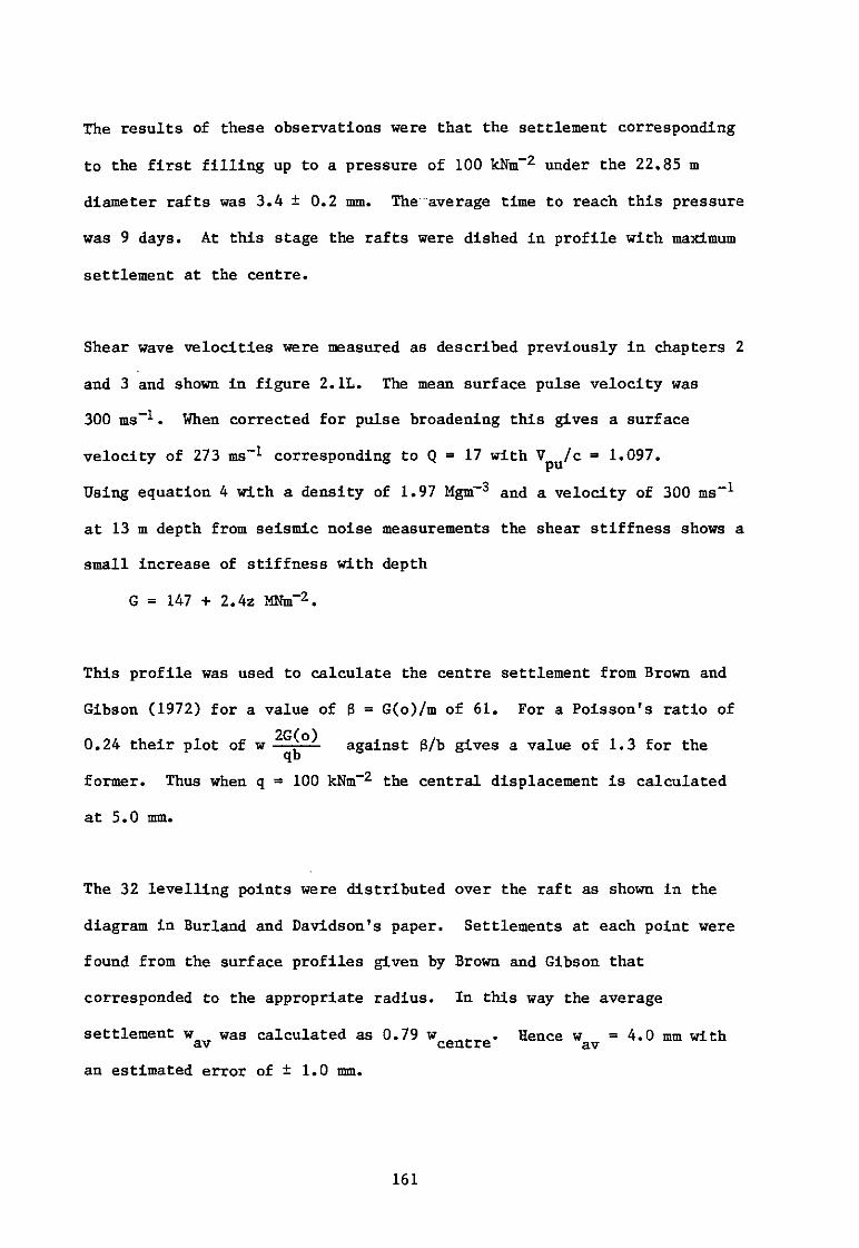
The results of these observations were that the settlement corresponding
to the first filling up to a pressure of 100 kNm"2 under the 22.85 m
diameter rafts was 3.4 ± 0.2 mm. The average time to reach this pressure
was 9 days. At this stage the rafts were dished in profile with maximum
settlement at the centre.
Shear wave velocities were measured as described previously in chapters 2
and 3 and shown in figure 2.1L. The mean surface pulse velocity was
300 ms"1. When corrected for pulse broadening this gives a surface
velocity of 273 ms""1 corresponding to Q = 17 with Vpu/c = 1.097.
Using equation 4 with a density of 1.97 Mgm~3 and a velocity of 300 ms""1
at 13 m depth from seismic noise measurements the shear stiffness shows a
small increase of stiffness with depth
G = 147 + 2.4z MNm"2.
This profile was used to calculate the centre settlement from Brown and
Gibson (1972) for a value of 8 = G(o)/m of 61. For a Poisson's ratio of
0.24 their plot of w against B/b gives a value of 1.3 for the qb
former. Thus when q = 100 kNm"2 the central displacement is calculated
at 5.0 mm.
The 32 levelling points were distributed over the raft as shown in the
diagram in Burland and Davidson's paper. Settlements at each point were
found from the surface profiles given by Brown and Gibson that
corresponded to the appropriate radius. In this way the average
settlement w was calculated as 0.79 w . . Hence w = 4.0 mm with av centre av an estimated error of ± 1.0 mm.
161
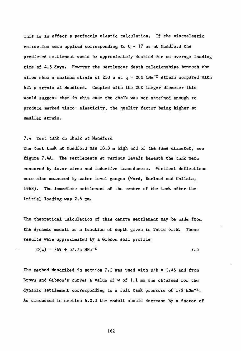
This is in effect a perfectly elastic calculation. If the viscoelastic
correction were applied corresponding to Q = 17 as at Mundford the
predicted settlement would be approximately doubled for an average loading
time of 4.5 days. However the settlement depth relationships beneath the
silos show a maximum strain of 250 y at q = 200 kNm"2 strain compared with
625 y strain at Mundford. Coupled with the 20% larger diameter this
would suggest that in this case the chalk was not strained enough to
produce marked visco- elasticity, the quality factor being higher at
smaller strain.
7.4 Test tank on chalk at Mundford
The test tank at Mundford was 18.3 m high and of the same diameter, see
figure 7.4A. The settlements at various levels beneath the tank were
measured by invar wires and inductive transducers. Vertical deflections
were also measured by water level gauges (Ward, Burland and Gallois,
1968). The immediate settlement of the centre of the tank after the
initial loading was 2.6 mm.
The theoretical calculation of this centre settlement may be made from
the dynamic moduli as a function of depth given in Table 6.2E. These
results were approximated by a Gibson soil profile
G(z) = 769 + 57.7z MNm"2 7.5
The method described in section 7.1 was used with 8/b = 1.46 and from
Brown and Gibson's curves a value of w of 1.1 mm was obtained for the
dynamic settlement corresponding to a full tank pressure of 179 kNm""2.
As discussed in section 6.2.3 the moduli should decrease by a factor of
162

Figure 7.4A Test tank, on chalk at Mundford
163
0.47 over a period of a day required for the tank filling and so the
calculated settlement becomes 2.3 mm, close to the observed value.
The effects of three dimensional consolidation on this site were
considered. The permeability of a cylindrical intact specimen of
Grade II chalk was measured in the laboratory using a constant head
permeameter. The mean value obtained was 4 x 10~8 ms""1 and this was
thought to represent a lower limit as the in situ values would be higher
due to fissuring.
The coefficient of three dimensional consolidation calculated was
2.6 x 10~3 s"1 m2 giving a time factor T y = 1.0 x 10~4 for h ~ 5 m. This
means that all consolidation effects would be over within a maximum of
three hours from the curves of Davis and Poulos. The creep curve given
by Burland and Lord (1969) shows little change over the time 0.1 to 1 day.
164
CHAPTER 8
CONCLUSION
Measuring the deformation properties of the ground is an example of the
classical mensuration problem of how to obtain information about a system
without disturbing it in some way. This is particularly true in the case
of stiff clays and weak rocks where most standard methods involve
sampling, or boring a hole for access. Geophysical methods which pass a
shear wave through the ground produce very little disturbance and so yield
low strain, in situ, information. The low strain, undisturbed,
deformation properties are often what is required in order to calculate
the strains occurring under a large foundation or around a large
excavation, where the strains are also small. The scale of the
measurement is quite large, about one wavelength of the shear waves, and
this often matches the scale of the system for which the information is
required.
The use of shear waves is found to be a great advantage as it frees the
calculation of modulus from the inherent lack of accuracy when the
Poisson's ratio is close to 0.5. Thus it is particularly suitable for
application to a stiff clay where this condition is found for short term
undrained measurements.
If the measurement is to be undisturbed and in situ, the shear wave
measurements must be made as a function of depth from the surface of the
ground. Three methods have been examined, shear wave refraction, surface
or Rayleigh wave methods and a new method involving seismic noise.
HFDAAM 165

The shear wave refraction survey has been developed with large horizontal
swing hammers that on some sites give a considerable depth of 20 m. By
summing the pulses, and reversing the polarity with the direction of the
swing hammers, both a reasonable degree of certainty that shear waves are
being observed, and a good signal to noise ratio, may be obtained. On
four out of five sites the method yielded Gibson soil properties that
increased with depth. Some correction may be applied for pulse
broadening, as it is a pulse technique, but this may not be as important
as other factors. With the present configuration this method yields
horizontal moduli. The best accuracy may be at a depth of 3 to 5 m
decreasing with depth below 5 m. The inversion of the time distance data
is carried out within experimental scatter on all five sites by curve
fitting with a linear increase of velocity with depth.
The Rayleigh wave experiment on the other hand yields velocities that are
controlled by moduli in both the vertical and the horizontal plane. Thus
the moduli may be more closely related to vertical settlements but the
problem is to obtain deep information. Measurements made with the
electromagnetic vibrator are restricted to the top few metres and the
mechanical vibrator gave a maximum depth of 12 m. Again signal to noise
ratio was the limiting factor. The velocities found tended to be smaller
than those from the pulse survey. The main problem with this experiment
is the interpretation of the correspondence of the velocity measured to a
depth of one half wavelength. There appears to be some confirmation of
this depth by the measurements made on the pit filled to a depth of one
metre. In practice the surface wave method was not so convenient to
deploy as the shear wave refraction survey.
166

The seismic noise technique which derives from the Rayleigh wave method
offers both rapid measurement and potentially great depths. It is easy
to deploy with a small amount of equipment required in the field. It does
depend upon the interpretation that part of the seismic noise is in the
form of horizontally travelling Rayleigh waves packets, but so far has
yielded velocities as a function of depth that are consistent within
experimental accuracy with other methods. At present a fair amount of
time is required for analysis of the seismic recordings in the laboratory
and the accuracy is not always as high as would be desired. However on
one site a standard deviation of ± 15% was obtained, for one depth only.
This method may benefit most from an improvement in analysis procedure.
On another site it yielded the greatest depth of 32 m.
For some situations at low strain a purely elastic treatment may be
sufficient, and at one site at least gave a correct value of settlement.
However for higher strain cases, especially in clays, time and strain
dependent effects must be taken into account. The model which has proved
most suitable has been that of the generalised viscoelastic solid with the
damping factor 1/Q fairly independent of time, but varying with strain
according to an fsf shaped curve against the logarithm of strain.
Fortunately the damping is not highly variable with strain. At worst it
doubles over a change of strain of a factor of ten. The theory has been
developed for the linear case and yields the useful result that the
logarithmic creep rate is proportional to (2/ir) times the damping factor
(1/Q). It appears that this can be applied as a first approximation to
the non linear case provided that the damping factor is found for the
level of strain at which the creep rate is required.
167

The fsf shaped curves of damping against strain appear to have a
consistent mathematical form that may reflect the way in which strain
dependent processes are activated as a function of strain.
The evidence for viscoelasticity in the ground is considerable. The most
conclusive is the measurement of damping or the complex part of the
modulus. Various in situ methods have been examined. The large scale
techniques tend to yield values that agree well with the published
laboratory values. On the other hand the small scale measurements from
hammer damping, and to a certain extent from plate resonance, tend to
lead to higher values of damping. The reason for this is discussed in
chapter 5 but it emphasises the difficulty of measuring the actual value
of strain at which the damping factor is obtained. These uncertainties
of measurement of in situ damping particularly at depth seem to be the
main contribution to the uncertainty in the moduli calculated. Methods
such as autocorrelation of seismic noise may yield in situ damping at
depth but they will be at a very low strain where it may be more difficult
to distinguish the different levels of damping. There appears to be no
direct way of telling whether one has a linear or a non linear material
apart from making damping measurements at various strains.
Comparisons with other in situ measurements of deformation parameters were
made at three sites, two on clay and one on chalk. At the first the
damping information came from the plate tests themselves with which the
comparison was made and so did indeed correspond to the strain level
required. At the other clay site published average damping data was
used and as in the other case corresponded to reloading conditions.
Agreement was reasonable at both these sites as a function of depth. At
168

the third site the only damping data available was from a small sample
tested in the laboratory, although indirect evidence pointed to similar
values. This in fact agreed with an in situ hammer test on another
similar chalk site although it was thought that the damping might well
vary with the grade of chalk as a function of depth. In all three cases
accuracies would have been improved if accurate in situ damping data could
have been obtained as a function of depth, which is not possible at
present.
The calculation of settlement, on a different set of three sites, was much
helped by the use of analytical methods that rely upon a Gibson soil model
with a linear increase of modulus with depth. This is close to the form
of the modulus variation found from the geophysical measurements.
At the first site on clay considerable time variation was observed, and
also predicted from high damping values found from hammer damping. Both
the high creep rate and high damping were thought to correspond to the
first loading case. Further settlement beyond one hour could be
calculated using three dimensional consolidation theory which continued
the curve obtained by viscoelasticity.
The second site on chalk apparently behaved elastically with an almost
zero increase of stiffness with depth and little or no time and strain
dependent effects below a certain level of strain. The foundations of the
silos in this case were large, perhaps even larger than the wavelengths
used.
169

The third site also on chalk gave a settlement that required a
viscoelastic correction although the high stiffness of this site was shown
by the high wave velocities measured. With the viscoelastic correction
good agreement was obtained with observed settlement.
Thus it would appear that these geophysical methods are of most value when
limited to the case of non plastic soils when the strains and deformations
to be calculated are small and the materials are well away from failure.
This is especially true for stiff clays and weak rocks where the moduli
are relatively high and the strains are small enough to be close to being
perfectly elastic.
As the strains for which the properties are required are increased so the
corrections to the low strain elastic properties become larger. Non
linear materials such as a clay may require a reduction of the modulus by
a factor of two or more. An in situ measurement of damping at known
strain, preferably close to the strain level for which the information is
required, enables the correction to be calculated by determining the
representative strain e^ for the material. At the moment various methods
of measuring damping have been applied but it is hoped that a method that
is universally applicable will evolve from this work.
The direction in which future work may proceed is indicated by experiments
in chapter 5. Low strain damping may indeed be accessible through auto-
correlation of seismic noise but much better statistical methods are
needed. Possibly the application of new computing techniques to handle
large numbers of samples will provide the solution. An alternative that
may obtain higher strain information may be the use of large impacts on
170

the surface produced either by dropping large weights or by arrays of
impactors. The latter may be coordinated electronically to produce
impacts over various areas thus obtaining information at various depths.
The small hammer damping measurement would benefit from a clarification
of the strains involved, perhaps by measuring the deformation of the
plate under the hammer blow. Improvements in damping measurement accuracy
would make the largest contribution to overall accuracy.
The theory of non linear viscoelasticity needs developing. The most
direct approach at the moment would be to measure the creep rate as a
function of strain for first, second, and subsequent loadings. The cone
and platen apparatus has been used to make some measurements with a
uniform strain throughout the specimen.
To complete the information on non linear viscoelasticity in clays the
damping factor 1/Q should be mapped as a function of strain at least
for London clay, Boulder clay and Gault clay. In addition the variation
of 1/Q with time should be measured both into the millisecond region
and out to periods of a day or more.
Developments of the three shear wave methods seem possible. Shear wave
refraction may benefit from deconvolution techniques allowing for the
change of pulse shape as it passes through the viscoelastic medium. The
Rayleigh wave technique may be improved by signal recovery methods that
average out the background noise. This would enable deeper information
to be obtained while still using moderately sized generators. The seismic
noise method would be improved by better statistics from a larger number
of samples and possibly from digital filtering with zero phase shifts.
171

Both improvements may come from the use of newer computers. Measurements
at greater depths are almost certainly possible and experiments are in
hand to use seismometers to reach a depth of half a kilometre.
172

REFERENCES
ABBISS, C P (1979): A comparison of the stiffness of the chalk at Mundford from a seismic survey and a large scale tank test. Geotechnique, 29, No 4, pp 461-468
ABBISS, C P (1981): Shear wave measurements of the elasticity of the ground. Geotechnique, 31. No 1, pp 91-104
ABBISS, C P (1983): Calculation of elasticities and settlements for long periods of time and high strains from geophysical measurements. To be published
ABBISS, C P and ASHBY, K D (1983): Determination of ground moduli by a seismic noise technique on land and on the seabed - technical note to be published
AMBRASEYS, N N and HENDRON, A J (1968): 'Dynamic behaviour of rock masses' ch 7 of Rock Mechanics in Engineering Practice, ed STAGG, K G and ZIENKIEWICZ, 0 C, J Wiley, New York
ATKINSON, J H and BRANSBY, P L (1978): 'The Mechanics of Soils', McGraw Hill, London
AWOJOBI, A 0 and GIBSON, R E (1973): Plane strain and axially symmetric problems of a linearly non homogeneous half-space. Q. Jnl. Mech. and Appl. Math. 26, Part 3, 285-302
BALLARD, R F and McLEAN, F G (1975): 'Seismic field methods for in situ moduli' Miscellaneous Papers S-75-10, US Army Engineer Waterways Experiment Station, Vicksburg, Miss 39180, USA
BISHOP, A W and HENKEL, D J (1957): 'The measurement of soil properties in the triaxial test'. London, Arnold
BLEANEY, B I and BLEANEY, B (1965): Electricity and Magnetism, Clarendon Press, Oxford
BOLTON SEED, H and IDRISS, I M (1970): Soil moduli and damping factors for dynamic response analyses. Report No EERC 70-10, Dec 1970. University of California, Berkeley
BORCHERDT, R D (1974): 'Rayleigh-type surface wave on a linear viscoelastic half-space' J Acoust Soc Am, 55, No 1, 13-15
BOUSSINESQ, J (1885): Application des Potentials a L'Etude de L'Equilibre et du Movement des Solides Elastiques. Gauthier Villars, Paris
BRADNER, H, DODDS, J G and FOULKS, R E (1965): Investigation of microseism sources with ocean-bottom seismometers. Geophysics, vol 30, No 4, pp 511-526
BROWN, P T and GIBSON, R E (1972): Surface settlement of a deep elastic stratum whose modulus increases linearly with depth. Canadian Geotechnical Journal 9, 467-476
HFDAAN 173
BROWN, P T and GIBSON, R E (1979): Surface settlement of a finite elastic layer whose modulus increases linearly with depth. International Journal for Numerical and Analytical Methods in Geomechanics 3 , 37-47
BROWN, P D and ROBERTSWAW, J (1953): The in situ measurement of Young's modulus for rock by a dynamic method. Geotechnique 283-286
BURLAND, J B (1983): - private communication
BURLAND, J B, BROMS, B B and de MELLO, V F B (1977): Behaviour of foundations and structures. Paper presented at 9th International Conference on Soil Mechanics and Foundation Engineering, Tokyo, July 1977. Session 2. BRE CP 51/78
BURLAND, J B and DAVIDSON, W (1976): A case study of cracking of columns supporting a silo due to differential foundation settlement. Conf. on Performance of Building Structures. Glasgow University, April 1976. Proceedings, Pentech Press, BRE CP 42/76
BURLAND, J B and HANCOCK, R J R (1977): Underground car park at the House of Commons, London: geotechnical aspects. Structural Engineer, Vol 55 (2) pp 87-100. BRE CP 13/77
BURLAND, J B and LORD, J A (1969): The load-deformation behaviour of Middle Chalk at Mundford, Norfolk. Proc Conf In Situ Investigation in Soils and Rocks, British Geotechnical Society, London. BRE CP 6/70
BURLAND, J B, MOORE, J F A and SMITH, P D K (1972): A simple and precise borehole extensometer. Geotechnique 22, pp 174-177
BURLAND, J B, SILLS, G C and GIBSON, R E (1973): A field and theoretical study of the influence of non-homogeneity on settlement. Proc. 8th Conf. of Intern. Soc. of Soil Mechanics and Foundation Engineering, Moscow. BRE, CP 32/73
BURLAND, J B and WROTH, C P (1974): 'Settlement of buildings and associated damage'. British Geotechnical Society's Conf. on Settlement of Structures, Cambridge, April 1974, Session 5, Proceedings pp 611-654. BRE CP 33/75
CHARLES, J A and WATTS, K S (1980): The influence of confining pressure on the shear strength of compacted rockfill. Geotechnique 30, No 4, pp 353-367
CHENEY, J (1973): Techniques and equipment using the surveyor's level for accurate measurement of building movement. British Geotechnical Society Symposium on Field Instrumentation, 30 May to 1 June 1973 at the Institute of Electrical Engineers, London
COGILL, W H (1974): SH- Waves in layered systems. Proc. First Australian Conference on Engineering Materials, University of New South Wales 1974, 529-545
Conference on settlement of structures, British Geotechnical Society, Cambridge, April 1974
174
COOKE, R W and PRICE, G (1973): Strains and displacements around friction piles. Proc. 8th Int Conf Soil Mech and Foundation Eng, Moscow, 2.1 pp 53-60. BRE CP 28/73
CUNNY, R W and FRY, Z B (1973): Vibratory in situ and laboratory soil moduli compared. Proc. ASCE 99, No SM 12, 1055-1076
DAVIS ANGELA (1978): A technique for the in situ measurement of shear wave velocity. ABEM printed matter No 90180, Bromma
DAVIS ANGELA and TAYLOR SMITH, D (1979): Dynamic elastic moduli logging of foundation materials. Proc. of a Conf on Offshore Site Investigation, Society for Underwater Technology, pp 121-132, March 1979, London
DAVIS E H and POULOS, H G (1968): The use of elastic theory for settlement prediction under three dimensional conditions. Geotechnique _18, 67-91
DEINUM, P J., DUNGAR, R., ELLIS, B R. , JEARY, A P., REED, G A L and SEVERN, R T (1982): Vibration tests on Emosson arch dam, Switzerland. Earthquake Engineering and Structural Dynamics JJ), 447-470
DRESCHER, A and DE JOSSELIN DE JONG, G (1972): Photoelastic verification of a mechanical model for the flow of a granular material. J. Mech. Phys. Solids 20, 337 to 351, Pergaman Press
DZIEWONSKI, A and HALES, A I (1972): Numerical analysis of dispersed seismic waves. Methods in Computational Physics, Academic Press, New York
EWING, W M, JARDETSKY, W S and PRESS, F (1957): 'Elastic waves in layered media' McGraw Hill, New York
FROOME, K D (1971): Mekometer III: EDM with sub-millimetre resolution. Survey Review 21, (July 1971), 98-112
GALLAGHER, K A (1980) - private communication
HARDIN, B 0 and DRNEVICH, V P (1972): Shear modulus and damping in soils: design equations and curves. J Soil Mechanics and Foundations Division, Proc of the American Society of Civil Engineers, Vol 98, SM 7, pp 667-692
HENDERSON, G, SMITH, P D K and ST JOHN, H D (1979): The development of the push in pressuremeter for offshore site investigation. SUT Conf on Offshore Site Investigation, 20-22 March, 1979, London
HEUKELOM, W and FOSTER, C R (1962): 'Dynamic testing of Pavements'. Trans Amer Soc Civil Eng. 127, 425-457
HORTON, C W (1953): 'On the propagation of Rayleigh waves on the surface of a viscoelastic solid'. Geophysics 18, 70-74
IYER, W M and HITCHCOCK, T (1976): Seismic noise survey in Long Valley, California. J Geophysics, Research, vol 81, No 5, pp 821-840
175
JONES, R (1958): In situ measurement of the dynamic properties of soil by vibration methods. Geotechnique J3, No 1, 1-21
KNOPOFF, L (1956): The seismic pulse in materials possessing solid friction I plane waves. Bull Seismological Society of America, Vol 46, pp 175-183
KULHANEK, 0 (1976): Introduction to digital filtering in geophysics. Elsevier, Amsterdam
LAMB, T W (1973): 'Prediction in soil engineering' Geotechnique 23, pp 151-202
LAMB, T W and WHITMAN, R V (1969): Soil Mechanics. Wiley, New York
LEITMAN, M J and FISHER, G M C (1973): 'The linear theory of viscoelasticity'. Mechanics of Solids III, Encyclopedia of Physics, Springer, Berlin
LOMNITZ, C (1956): Creep measurements in igneous rocks. J Geol Vol 64, pp 473-479
LOMNITZ, C (1957): Linear dissipation in solids. J of Applied Physics, Vol 28, No 2 pp 201-205
LOMNITZ, C (1974): Global tectonics and earthquake risk. Elsevier, Amsterdam
LYSMER, J (1970): Lumped mass method for Rayleigh waves. Bull. Seism. Soc. Am. 60, No 1, 89-104
MARSLAND, A (1971)a: Laboratory and in-situ measurements of the deformation moduli of London clay. Proc Symp on Interaction of Structure and Foundation. Midland Soil Mech and Foundation Eng. Soc, Dept of Civ Eng. University of Birmingham, July 1971 (also BRE Current Paper CP 24/73)
MARSLAND, A (1971)b: 'Large in-situ tests to measure the properties of stiff fissured clays'. First Australian-New Zealand Conf on Geomechanics Melbourne, 1971, Proc. Vol j , 180-189. BRE CP 1/73
MARSLAND, A and EASON, J E (1973): Measurement of displacements in the ground below loaded plates in deep boreholes. Brit Geot Soc Symp on Field Instrumentation in Geotechnical Engineering, Butterworths, London
MAXWELL, A A and FRY, Z B (1967): A procedure for determining elastic moduli of in-situ soils by dynamic techniques. Proc Int Symp on Wave Propagation and Dynamic Properties of Earth Materials, ASCE, Soil Mech and Foundation Div. Univ of New Mexico Press, Alberquerque, USA
MILLER, G F and PURSEY, H (1954): Field and radiation impedance of mechanical radiators on the free surface of a semi infinite isotropic solid. Proc Roy Soc, A, Vol 223, pp 521
MILLER, G F and PURSEY, H (1955): On the partition of energy between elastic waves in a semi-infinite solid. Proc Roy Soc A Vol 233, pp 55-59
176
MOONEY, H M (1974): Seismic shear waves in engineering, ASCE Proc, vol 100, No GT8, pp 905-923
MOONEY, H M (1976): The seismic wave system from a surface impact. Geophysics 41, No 2 (April 1976), 243-265
MORRIS, D V and ABBISS, C P (1979): 'Static modulus of Gault clay predicted from seismic tests'. Ground Engineering 12, No 8, 44-50
NETTLETON, L L (1940): Geophysical prospecting for oil. London, McGraw Hill
NOWICK, A S and BERRY, B S (1972): Anelastic relaxation in crystalline solids. Academic Press, London
PILANT, W L (1979): 'Elastic waves in the earth'. Developments in solid earth geophysics, Elsevier, Amsterdam
RAYLEIGH, LORD (1900): On waves propagated along the plane surface of an elastic solid. Scientific papers of Lord Rayleigh, Vol 2, 441-447, London, Cambridge University Press
RICKER, N H (1977): Transient waves in viscoelastic media. Elsevier, Amsterdam
ROESLER, S (1977): Correlation methods in soil dynamics. Proc Dynamic methods in soil and rock mechanics. Karlsruhe, Sept 1977, Vol 1, pp 309-334. Balkema, Rotterdam
R0US0P0UL0S, A A (1978): Seismic regionalisation techniques and strong motion recordings. MPhil thesis, University of London
ST JOHN H D (1975): Field and theoretical studies of the behaviour of ground around deep excavations in London clay, PhD thesis, Cambridge University
SAMUELS, S G (1975): Some properties of the Gault clay from the Ely-Ouse Essex water tunnel. Geotechnique 25, No 2, 239-264
SCHWAB, F and KNOPOFF, L (1972): Fast surface wave and free mode computations. In BOLT B A (Editor) Methods in computational physics Vol II, Seismology: surface waves and earth oscillations. Academic, New York pp 87-180
SMITH, P D K and BURLAND, J B (1976): Performance of a high precision multi-point borehole extensometer in soft rock. Canad. Geotechnical Journal 13, No 2, pp 172-176
WAKELING, T R M (1974): Discussion on Session IV 'Rocks' pp 748-750 Proc. Conf on Settlement of Structures. Cambridge, Pentech Press 1975
WARD, W H and BURLAND, J B (1973): The use of ground strain measurements in civil engineering. Phil. Trans. R Soc. Land. A 274, 421-428
177

WARD, W H, MARSLAND, A and SAMUELS, S G (1965): Properties of the London clay at the Ashford Common shaft: In-situ and undrained strength tests. Geotechnique _15, 321-344
WHITE, J E (1965): Seismic waves, radiation transmission and attenuation. McGraw Hill, New York
WHITMARSH R B and LILWALL, R C (1982): A new method for the determination of in-situ shear wave velocity in deep-sea sediments. Oceanology International 1982, March 2nd-5th, Brighton, England
WINDLE, D (1976): In situ testing of soils with a self-boring pressuremeter. PhD Thesis, Cambridge University
WOODS, R D and RICHART, F E (1967): Screening of elastic surface waves by trenches. Proc. Int Symp on Wave propagation and dynamic properties of earth materials. ASCE Soil Mech and Found Dv, University of New Mexico Press, Alberquerque, USA
178

APPENDIX I
This derivation of the properties of the generalised viscoelastic solid
largely follows Nowick and Berry with some additions
The standard anelastic solid.
This has three elements a, b, c
e = e + £, , £, = £ a b' b e
a = o = J £ = a, + a = 6J-1 (e, + re ) a u a b c b c
eliminating terms in a, b, c
Jno + t J a = £ + x £ R a u a where
J R = J u + SJ is the relaxed compliance
This is the differential stress strain equation of the three parameter
model
for t > 0 with
o = o . 6 = 0 t > 0 o* e = J o at t = 0 u
Now the solution of y + ty = c
. ^ A -t/T is y = c + Ae
J(t) - - JR - (j -j ) exp (-t/t0 ) O
J(t) = Ju + 5j[l - exp (t/ta )1
FZRAAR 179
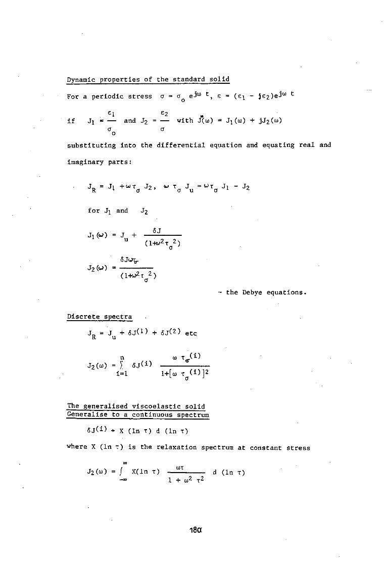
Dynamic properties of the standard solid
For a periodic stress a = Oq e ^ e = (e^ - je2)ejw t
if Ji - — and J2 = — with J(u)) = Jx(u)) + jJ2(o>) a a o
substituting into the differential equation and equating real and
imaginary parts:
J_ = Jx +wt J2, v t J = Ut Jx - J2 R 1 a a u a
1
for Jx and J2
5 J Jl(u>) = J +
j 2 m -
U (H«2X 2) a SJu^r (1+u>2t 2) a
- the Debye equations
Discrete spectra
J_ = J + 5jO> + 6j(2) etc R u
J2(u)> = I SjC1) n u> t (I)
i=l l+[u> T (i)]2
The generalised viscoelastic solid Generalise to a continuous spectrum
5j(i) X (ln t) d (ln t) where X (ln x) is the relaxation spectrum at constant stress
J2(w) = / X(ln x) — — d (ln x) 1 + 0)2 T2
610

Constant spectrum X
, v R WT , . J2(o)) = / X d In T 1 + U)2 X2
= x 0) / —tk. O 1 + 0 ) 2 T 2
oo X I tan"1 (TW)| = - X
o 2
J2(y) - j x y l s l n a)~1
1 _ J 2 _ TT X Q JX 2 JJ_
For a spectrum approximately constant over the range of a Debye peak
2 JiCrn) X(oi) = -¥ Q(0)>
Alfrey1s rule
For a multiple element system summing strains
n J(t) = Ju + I [i - exp (- t/r C1))]
u i=l a
from the definition of a continuous spectrum
00 J(t) = Ju + / X (In T) [l - exp (- t/x) ] d ln T
—oo
y = ln t, t = eX, z = ln x, x = ez
oo J(y) - J u - / x(2) [i - exp (- ey-z)l dz
—oo
Now [l - exp (- e^"2)] is a steplike function, unity for z « y
and zero for z » y.
181
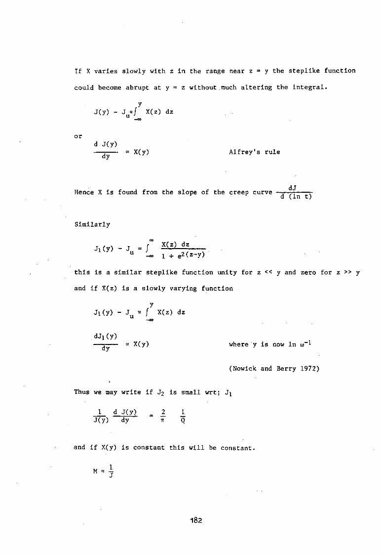
If X varies slowly with z in the range near z = y the stepiike function
could become abrupt at y = z without.much altering the integral.
y J(y) - J * J X(z) dz
or d J ( y )
= X(y) Alfrey's rule dy
Hence X is found from the slope of the creep curve d (ln t)
Similarly
X(z) dz Ji(y) - J = / x •
u _oo 1 + e2Cz-y)
this is a similar steplike function unity for z << y and zero for z >> y
and if X(z) is a slowly varying function y
Ji(y) - J u * / X(z) dz -oo
d J i ( y ) — ^ — - X(y) where y is now ln aT"1
(Nowick and Berry 1972)
Thus we may write if J2 is small wrt; J^
1 d J(y) 2 _1 J(y) dy TT Q
and if X(y) is constant this will be constant.
182

dM(y) M dy
_2 TTQ
2/ttQ
or M2 = Mi ©
183
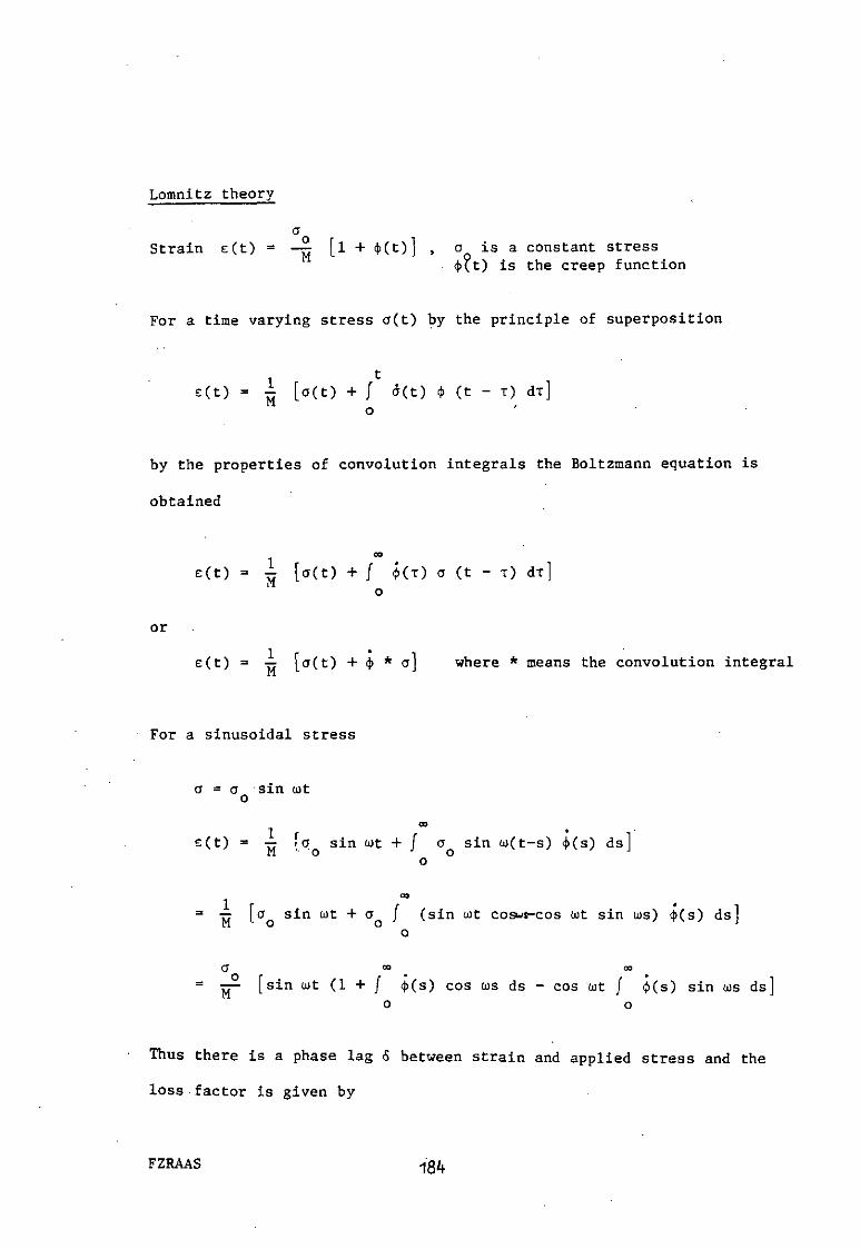
Lomnitz theory
a Strain e(t) = —~ [l + <KO] , a is a constant stress
<j> t) is the creep function
For a time varying stress o(t) by the principle of superposition
. t e(t) = i [o(t) + J a(t) <f> (t - T ) dx] M o
by the properties of convolution integrals the Boltzmann equation is
obtained
e(t) = | [a(t) + / i(x) a (t - x) dx] o
or 1 r * i
E(t) = — c(t) + 6 * a where * means the convolution integral M
For a sinusoidal stress
0 = a sin tot o 00
£(t) = — [or sin tot + / 0 sin co(t-s) Ks) ds] o
1 °° = sin o)t + a / (sin cut cosws-cos cot sin cos) $(s) ds] o
O 00 00
= yp [sin cot (1 + / <£(s) cos tos ds - cos cot / <£(s) sin cos ds] o o
Thus there is a phase lag 6 between strain and applied stress and the
loss factor is given by
FZRAAS 134.
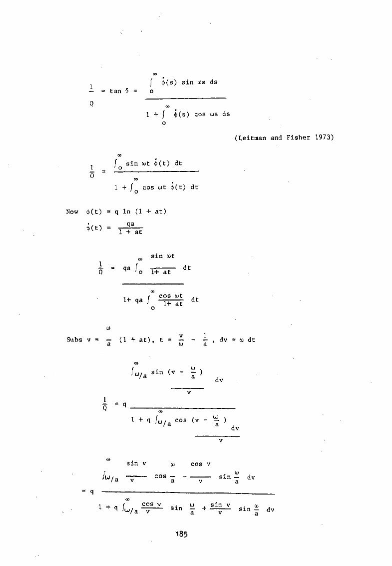
1 X — = tan o = o | <Ks) s in cas ds
. » 1 + J 4>(s) cos cas ds
o (Leitman and Fisher 1973)
CO f s in cat F t ) dt 1 J o
0 1 + / cos cat F t ) dt J o
Now 4>(t:) = q ln (1 + at) qa F O = 1 + at
sin cat
Q = q a / o I T S — d t
f cos cat , 1 + q a j t t s t d t o
ca v 1 Subs v = — (1 4- at), t = — - — , dv = ca dt a ' ca a
f u / a sin (v - j ) dv
Q = q
1 + q /<J/a c o s ( v - 7 ) dv
sin v u) cos v
^ / a T C O S a * v S i n I d v
= q —
l 4- n f c o s v ca , s in v . aj q M a s i n ~ + — ~ — sin - dv a v a
185

Integral functions:
s l ( x ) = / dv, Si(«) = J , Ci(x) = V J O V I.
- 1 . COS
\
¥ _ 0) \ W . Ill j W — - Si — \ cos — + Ci — sin —
1 + q — - Si — sin — - Ci — cos — \ 2 a / a a a
if a is large
Q " 7 q
186
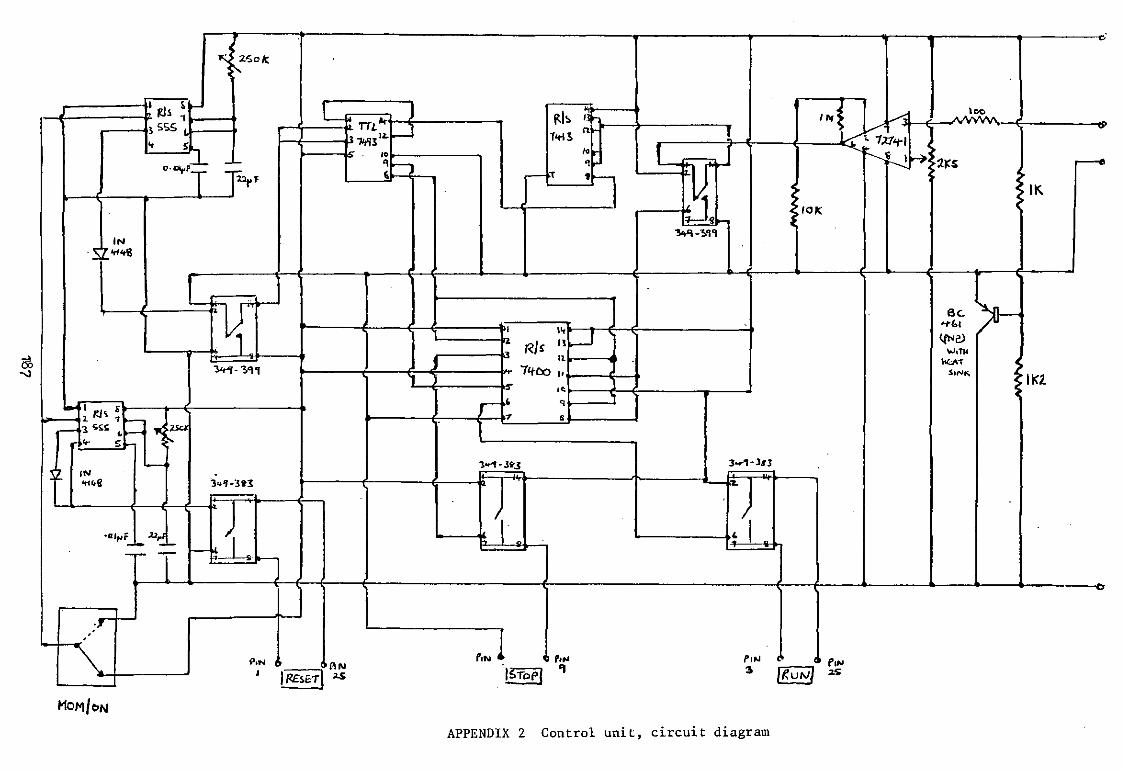
H O M / O N
APPENDIX 2 Control unit, circuit diagram

APPENDIX 3 - CALCULATOR PROGRAHS
I. TO FIND k FRO}! . h kT S1n 2 FIT. FIRST ESTI!-LI\TE FROH 2 POINTS
LBLA enter tl RCLO X
STO 0 RCL] PSE
RTN STOO F?O
LBL B enter t2 30 RV R/5
CFO STOI SFO
CFI SFI 2 dec k by 5
STOI G TO C
LBL E LBLD 60 5
5 ST05 STO-2
10 STO+2 RCLO G TO C
LBLC RCLI LBlLl:
RCL2 STOO F?O
RCLO RV G TO b inc k by 5
X 40 STOI 2
SI03 calc CF 1
x sinh kJ RCLS 5 e
RCL3 RCL4 5TO+2
CHS 70 G TO C
x 2 LBLb e
20 inc k by O.
2 P5E 2
5
PSE Y < x STO+2
F?l 50 G TO a G TO C
G TO D RCL2 77 R/S
ST04 2
188

BEST LINEAR FIT OF sin/z
LBLA
DSP6
STOA
CF1
RTN
LBLB
2
STOB
RTN
LBLC
ISZ RCI RTN LBLD 0
STI
LBLa
RCL(i)
RCLB
X
STOC x e
RCLC
CHS jc
Store Ad
Store k
Stores T
STO+(i) in reg 0-9
(10 units)
GO
calc
sinh kt
kT_ _ kd
2 ~ 2 V o
30
BY LINEAR REGRESSION
40
50
STOD
ISZ
SPC
RCI
RCLA
X
RCLD
x < y
X +
9
RCI
x <: y
G TO a P > S
RCL8
RCL4
RCL6
X
RCL9
ENT+
ENT+
RCL4 •7
x
RCL9
finds stat.values
to- s n
189

60
RCL5
x t y
STOC
X
RCL6
x2
RCL9
Ex-
Stores b (slope)
ay)
90
STOB
RV
STOA
RV
STOE P > S
0
STI
RCLB
0 inc. k by 1
70
80
CHS
RCL7
-x-
F? 1
GSB2?
RCLE
x < y
GSBcZ
RCLB
1
STOB
SFl
LBLd
RV
RCLA
RCLB
CLREG
ay1)
tests for dec
in k
tests r2
if r2 < r2prev.
retn to prev. k
clear stat
calcns
100
110
STOB
G TO D
LBLZ?
STOE
R/S
LBL E
RCLE
-x-
RCL B
2 X
-x-
RCLC
-x-
RCL6
Results
K
190

RCL4
120 RCLC
X
RCL9
-x- a intercept
126 R/S
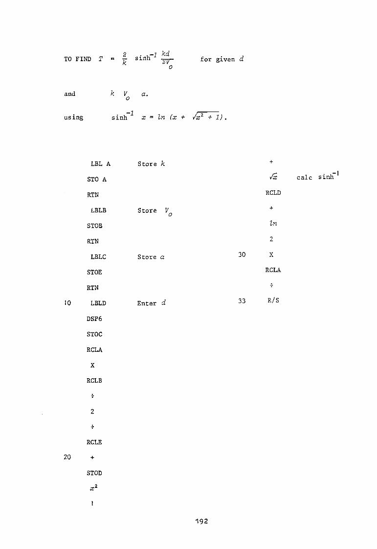
2 • .-i kd . TO FIND T = ^ sinh f o r given d o
and k V a. o
using sinh 2 x = In (x + /x2 + 1) .
10
LBL A
STO A
RTN
LBLB
STOB
RTN
LBLC
STOE
RTN
LBLD
DSP6
STOC
RCLA
X
RCLB
Store k
Store V
Store a
Enter d
+
/x
RCLD
calc sinh 1
30
In
2
X
RCLA
33 R/S
2
RCLE
20 +
STOD
1
192

MAXIMUM DEPTH Finds z max
max v o k 1 + kti
2V
2 I - 1
LBL A (k)
STO 0
RTN
LBL B (F ; o
STO 1
RTN
LBLC (d)
STO 2
RCLO
10 X
RCL 1
RCLO
RTN
20
1 +
/x
1
RCL 1
X
195
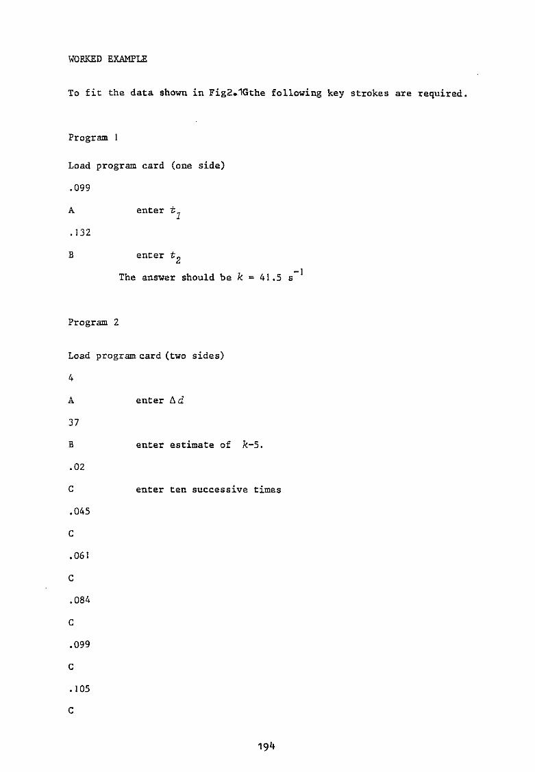
WORKED EXAMPLE
To fit the data shown in Fig2.1Gthe following key strokes are required.
Program l
Load program card (one side)
.099
A enter t^
.132
B enter t^
The answer should be k = 41.5 s 7
Program 2
Load program card (two sides)
4
A enter Ad
37
B enter estimate of k-5.
.02
C enter ten successive times
.045
C
.061
C
.084
C
.099
C
.105
C
194
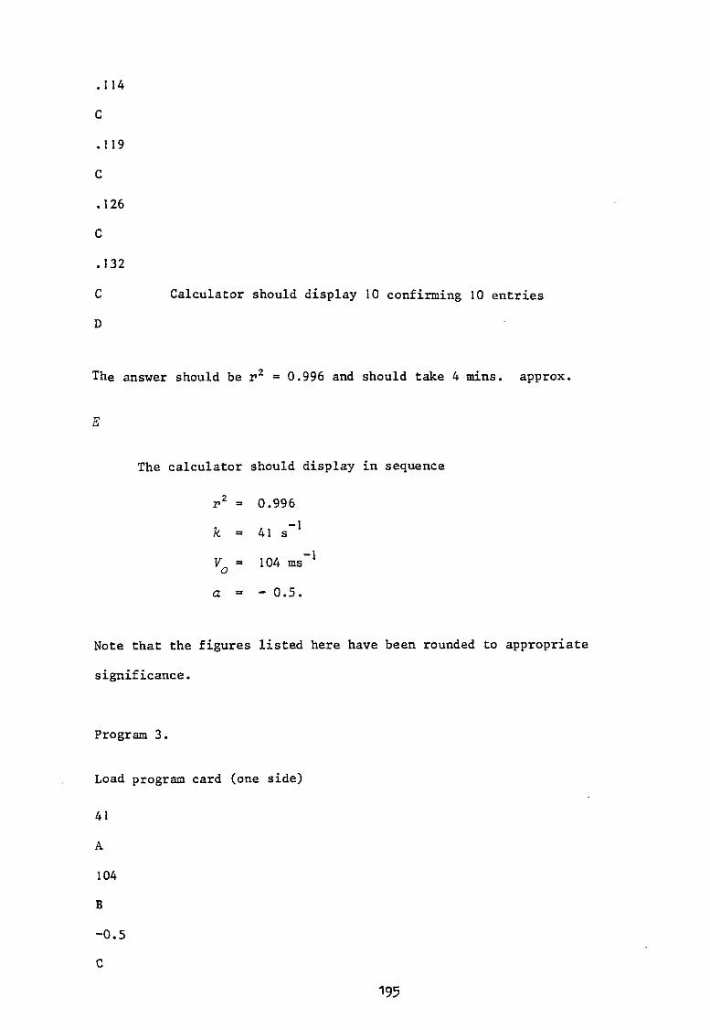
.114
C
.119
C
.126
C
.132
C Calculator should display 10 confirming 10 entries
D
The answer should be r2 = 0.996 and should take 4 mins. approx.
E
should display in sequence
0.996
41 s"1
104 ms"1
- 0.5.
Note that the figures listed here have been rounded to appropriate
significance.
Program 3.
Load program card (one side)
41
A
104
B
-0.5
C
195
The calculator
r 2
k =
V o m
a =

20
D
The answer should be 0.095 s and similarly the time may be found for any
other distance.
Program 4.
Load program card (one side)
41
A
104
B
40
C
The answer should be 17.6 m.
196

Program for time dependence of the modulus (H.P 67)
1 FLBLA TT X h 17X 2 X STOO hRTN fLBLB
10 ST01 hRTN fLBLC ST02 hRTN fLBLD ST03 hRTN fLBLE RCL1
20 RCL2
RCLO hyx
RCL3 X hRTN
197
Recommended


![Arc parallel shear deformation and escape flow in the ...as GPS deformation measurements or temperature and flow modeling at depth. [10] Based on the joint consideration of the results](https://img.pdfslide.us/doc/110x75/5e9a6f2ecf9782594a446f6b/arc-parallel-shear-deformation-and-escape-flow-in-the-as-gps-deformation-measurements.jpg)