Selected Topics in Robust ConvexOptimization
Arkadi Nemirovski
School of Industrial and Systems Engineering
Georgia Institute of Technology
• Optimization programs with uncertain data and theirRobust Counterparts
• Tractability of Robust Counterparts• Robust Optimization and Chance Constraints
• Optimization programs with uncertain data and theirRobust Counterparts
• Tractability of Robust Counterparts• Robust Optimization and Chance Constraints
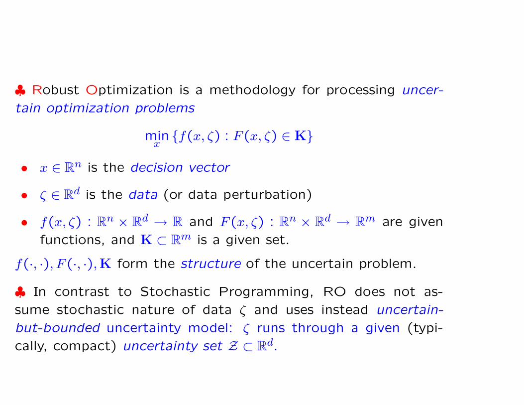
♣ Robust Optimization is a methodology for processing uncer-
tain optimization problems
minx
{f(x, ζ) : F (x, ζ) ∈ K}
• x ∈ Rn is the decision vector
• ζ ∈ Rd is the data (or data perturbation)
• f(x, ζ) : Rn × Rd → R and F (x, ζ) : Rn × Rd → Rm are given
functions, and K ⊂ Rm is a given set.
f(·, ·), F (·, ·),K form the structure of the uncertain problem.
♣ In contrast to Stochastic Programming, RO does not as-
sume stochastic nature of data ζ and uses instead uncertain-
but-bounded uncertainty model: ζ runs through a given (typi-
cally, compact) uncertainty set Z ⊂ Rd.

♣ RO, people:
• 1973: A.L. Soyster (LP)
• 1997: P. Kouvelis & G. Yu (IP)
• 1997 –:L. El Ghaoui & H. Lebret & F. OustryA. Ben-Tal & A. Nemirovski
}
(CP)
• 2000 –: E. Adida, A. Atamturk, A. Beck, D. Bertsi-
mas, C. Bhattacharyya, H.-G. Bock, S. Boyd, G. Calafiore,
M. Diehl, Y. Eldar, E. Erdogan, L. Grate, E. Guslitzer,
B. Golany, D. Goldfarb, C. Hol, G. Iyengar, M. Jor-
dan, E. Kostina, O. Kostyukova, G. Lanckriet, A. Nilim,
M. Sim, D. Pachamanova, C. Roos, C. Schrerer, A. Sood,
A. Thiele, J.-Ph. Vial, M. Zhang,...
♠ RO, applications:• Structural/Circuit/Network Design • Control • Signal
Processing • Machine Learning • Portfolio Optimization
• Inventory...

Example of uncertain LP: Multi-product inventory with back-
logged demand and shared warehouse capacity
minC,xt,yt,wt,vt
C [inventory management cost]
s.t.∑T
t=1[c′hyt + c′bwt + c′pvt] ≤ C [cost description]
xt+1 = xt + vt − ζt [balance equations]
xt ≤ yt, 0 ≤ yt [bounds on [xt]+]
−xt ≤ wt, 0 ≤ wt [bounds on backlogged demand]
vt ≤ vt ≤ vt [bounds on orders]
q′yt ≤ Q [warehouse capacity bound]
• xt ∈ Rd: inventory state at time t • q ∈ Rd+: storage requirements
• vt ∈ Rd: replenishment orders at time t • co ∈ Rd+: ordering costs
• yt ∈ Rd: stored items at time t • ch ∈ Rd+: holding costs
• wt ∈ Rd: backlogged demand at time t • cb ∈ Rd+: backlog penalty
• Uncertain data: demands ζ = [ζ1; ...; ζT ]

{
minx
{f(x, ζ) : F (x, ζ) ∈ K} : ζ ∈ Z}
(Unc)
Assume that our “decision environment” is such that
• All decisions xj should be made before ζ “reveals itself”
and thus should be independent of ζ
• The constraints are “hard”: their violations cannot be
tolerated
• We intend to take full care of all data ζ ∈ Z and do not
care what happens when ζ 6∈ Z.
Under these assumptions, seemingly the only meaningful way to
process (Unc) is to solve the Robust Counterpart
mint,x
{t : ∀ζ ∈ Z : f(x, ζ) ≤ t, F (x, ζ) ∈ K} (RC)
of the uncertain problem.
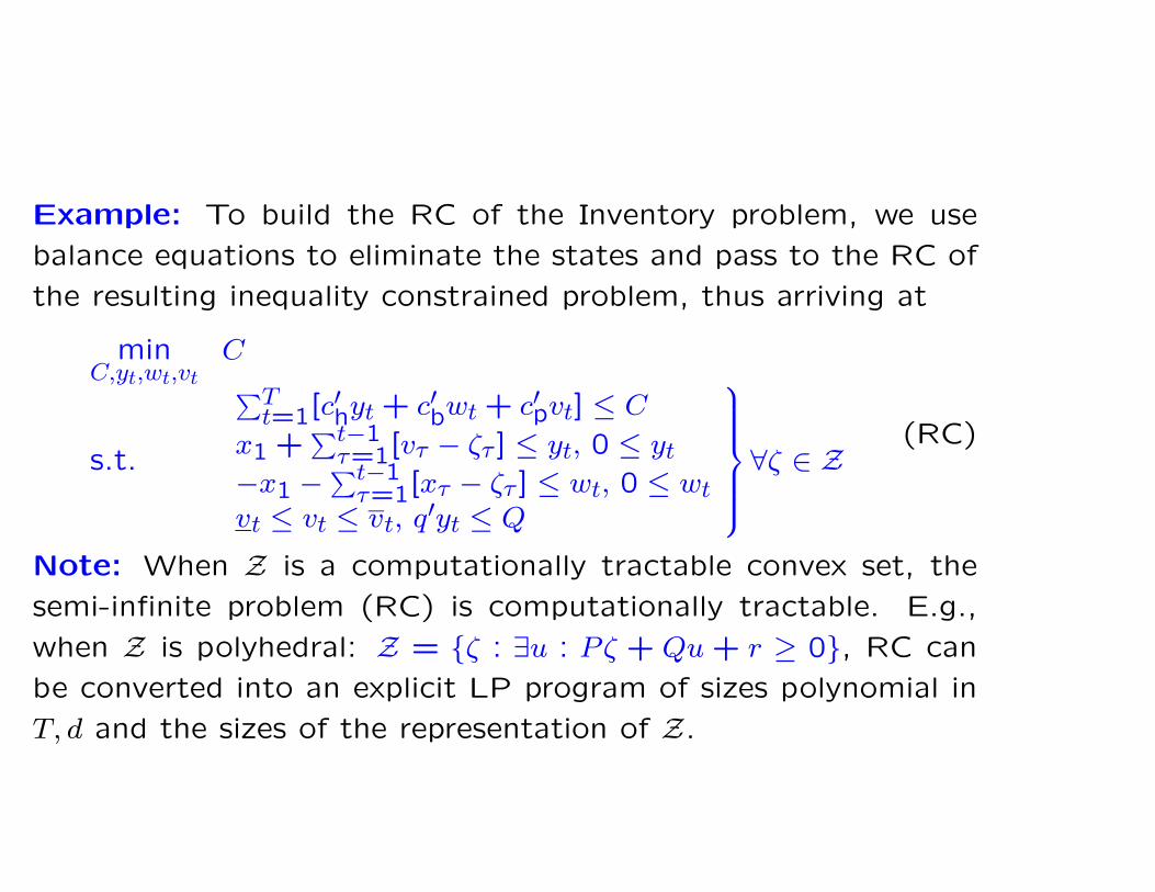
Example: To build the RC of the Inventory problem, we use
balance equations to eliminate the states and pass to the RC of
the resulting inequality constrained problem, thus arriving at
minC,yt,wt,vt
C
s.t.
∑Tt=1[c
′hyt + c′bwt + c′pvt] ≤ C
x1 +∑t−1
τ=1[vτ − ζτ ] ≤ yt, 0 ≤ yt
−x1 − ∑t−1τ=1[xτ − ζτ ] ≤ wt, 0 ≤ wt
vt ≤ vt ≤ vt, q′yt ≤ Q
∀ζ ∈ Z(RC)
Note: When Z is a computationally tractable convex set, the
semi-infinite problem (RC) is computationally tractable. E.g.,
when Z is polyhedral: Z = {ζ : ∃u : Pζ + Qu + r ≥ 0}, RC can
be converted into an explicit LP program of sizes polynomial in
T, d and the sizes of the representation of Z.

♣ Extending the notion of RC: Adjustable/Affinely Adjustable
Robust Counterpart.
♠ Assumption “All decisions xj should be independent of ζ” is
too restrictive in many applications:• Some of xj are “analysis variables” which do not represent
decisions at all and can therefore depend on the entire data.
Examples: • Converting the constraint∑
i |aTi x − bi| ≤ t
with uncertain ai, bi into −yi ≤ aTi x − bi ≤ yi,
∑
i yi ≤ t,
it is natural to allow the analysis variables yi to “adjust
themselves” to the actual data.
• In the Inventory problem, the actual decisions are the
replenishment orders vt and the inventory management
cost C; the remaining variables xt, yt, wt are analysis ones,
and we can allow these variables to “adjust themselves”
to the actual data.

• In dynamical decision-making, some of the decisions xj should
be made when the actual data becomes partially known and thus
can depend on the corresponding portions of the data
Example: In the Inventory problem with uncertain de-
mand, replenishment orders vt of day t usually can depend
on the actual demands at days 1, ..., t − 1.

♣ To account for adjustability, we allow for every xj to depend
on a prescribed portion Pjζ of ζ: xj = Xj(Pjζ), thus arriving at
Adjustable Robust Counterpart
mint,{Xj(·)}n
j=1
{t : ∀ζ ∈ Z : f(X(ζ), ζ) ≤ t, F (X(ζ), ζ) ∈ K}
[X(ζ) = {Xj(Pjζ)}](ARC)
Note: ARC is infinite-dimensional and thus is typically heavily
computationally intractable. Seemingly the only applicable tech-
nique is Dynamic Programming ⇒“curse of dimensionality”
♣ To overcome, to some extent, intractability of ARC, we re-
strict the decision rules to be affine: Xj(Pjζ) = ξ0j + ξTj Pjζ, thus
arriving at the Affinely Adjustable Robust Counterpart
mint,{ξ0j ,ξj}n
j=1
{t : ∀ζ ∈ Z : f(X(ζ), ζ) ≤ t, F (X(ζ), ζ) ∈ K}
[X(ζ) = {ξ0j + ξTj Pjζ}n
j=1](AARC)

Example: The only “actual decisions” in the Inventory problemare orders vt. Assume that vt can depend on the precedingdemands ζt−1 = [ζ1; ...; ζt−1]. To build the AARC, we• introduce linear decision rules for the orders vt = v0
t + Vtζt−1
• make xt, yt, wt affine functions of ζ:xt = x0t + Xtζ, yt = y0
t +Ytζ, wt = w0
t + Wtζ, thus ending up with
minC,v0
t ,Vt,...,w0t ,Wt
C
s.t.
∑
t≤T [c′h[y0t + Ytζ] + c′b[wt + Wtζ] + c′p[v
0t + Vtζt−1]] ≤ C
x0t+1 + Xt+1ζ = x0
t + Xtζ + v0t + Vtζt−1 − ζt
x0t + Xtζ ≤ y0
t + Ytζ, 0 ≤ y0t + Ytζ
−[x0t + Xtζ] ≤ w0
t + Wtζ, 0 ≤ w0t + Wtζ
vt ≤ v0t + Vtζt−1 ≤ vt, q′[y0
t + Ytζ] ≤ Q
∀ζ ∈ Z
(AARC)Note: The AARC of the Inventory problem is computationallytractable provided that Z is so. E.g., when Z is a polyhedral set,(AARC) is equivalent to an explicit LP program.

Example (continued): Consider single-product Inventory with
N = 10 and a box uncertainty set: (1 − ρ)ζn ≤ ζ ≤ (1 + ρ)ζn.
Here the ARC is well within the grasp of Dynamic Programming.
♣ How large are the gaps in the chain Opt(ARC) ≤ Opt(AARC) ≤Opt(RC) ?
• We built a sample of 768 Inventory problems with uncertainty
of 10% – 50% by picking at random cost coefficients, storage
capacity and nominal demand trajectory ζn and subsequent fil-
tering out problems with infeasible ARC’s.
♠ It turns out that Opt(ARC) = Opt(AARC) in every one of
these 768 problems!
Note: This phenomenon disappears when passing from minimiz-
ing the worst-case inventory management cost to minimizing the
average of this cost.

♠ Opt(RC) was typically essentially worse than Opt(ARC) =
Opt(AARC):
Range of Opt(RC)
Opt(ARC)1 (1,2] (2,10] (10,1000] ∞
Frequency in the sample 38% 23% 14% 11% 15%
♣ In the RO context, affine decision rules not necessarily are
bad!

• Optimization programs with uncertain data and theirRobust Counterparts
• Tractability of Robust Counterparts• Robust Optimization and Chance Constraints

♣ Robust Counterparts of uncertain problem are semi-infinite
programs and thus can be intractable even when all instances of
the uncertain problem are easy to solve.⇒ When Robust Counterparts are computationally tractable?
What to do if it is not the case?

♠ We focus on uncertain affinely perturbed LP/CQP/SDP prob-
lems{
minx
{
cTζ x + dζ : Ai
ζx + biζ ∈ Ki, i = 1, ..., m
}
: ζ ∈ Z}
with fixed recourse:
• cζ, dζ, Aiζ, b
iζ: affine in ζ
• Fixed recourse [automatically valid for the RC]: All coeffi-
cients of the adjustable variables xj (those with Pj 6= 0) are
certain (i.e., independent of ζ).
• Ki: nonnegative rays/Lorentz cones/semidefinite cones (un-
certain LP, CQP, SDP, respectively).
♠ We always assume that Z is given by a strictly feasible semidef-
inite representation
Z = {ζ : ∃u : P(ζ, u) � 0}(P(·): affine in (ζ, u)).

♣ Investigating tractability of Robust Counterparts of uncertain
affinely perturbed LP/CQP/SDP problems with fixed recourse
reduces to investigating tractability of semi-infinite affinely per-
turbed conic inequalities
∀ζ ∈ Z : Aζx + bζ ∈ K =
nonnegative ray [Uncertain LP]Lorentz cone [Uncertain CQP]semidefinite cone [Uncertain SDP]
[
Aζ, bζ: affine in ζ]

♣ Tractability of a semi-infinite affinely perturbed conic inequal-
ity
∀ζ ∈ Z : Aζx + bζ ∈ K
depends on the tradeoff between the geometries of K and Z –
the more complicated is Z, the simpler should be K.
♣ “Trivial case”: Scenario-generated uncertainty set
Theorem. The RC/AARC of an uncertain affinely perturbed
LP/CQP/SDP problem{
minx
{
cTζ x + dζ : Ai
ζx + biζ ∈ Ki, i = 1, ..., m
}
: ζ ∈ Z}
with fixed recourse and with scenario-generated uncertainty set
Z = Conv{ζ1, ..., ζN} is computationally tractable.
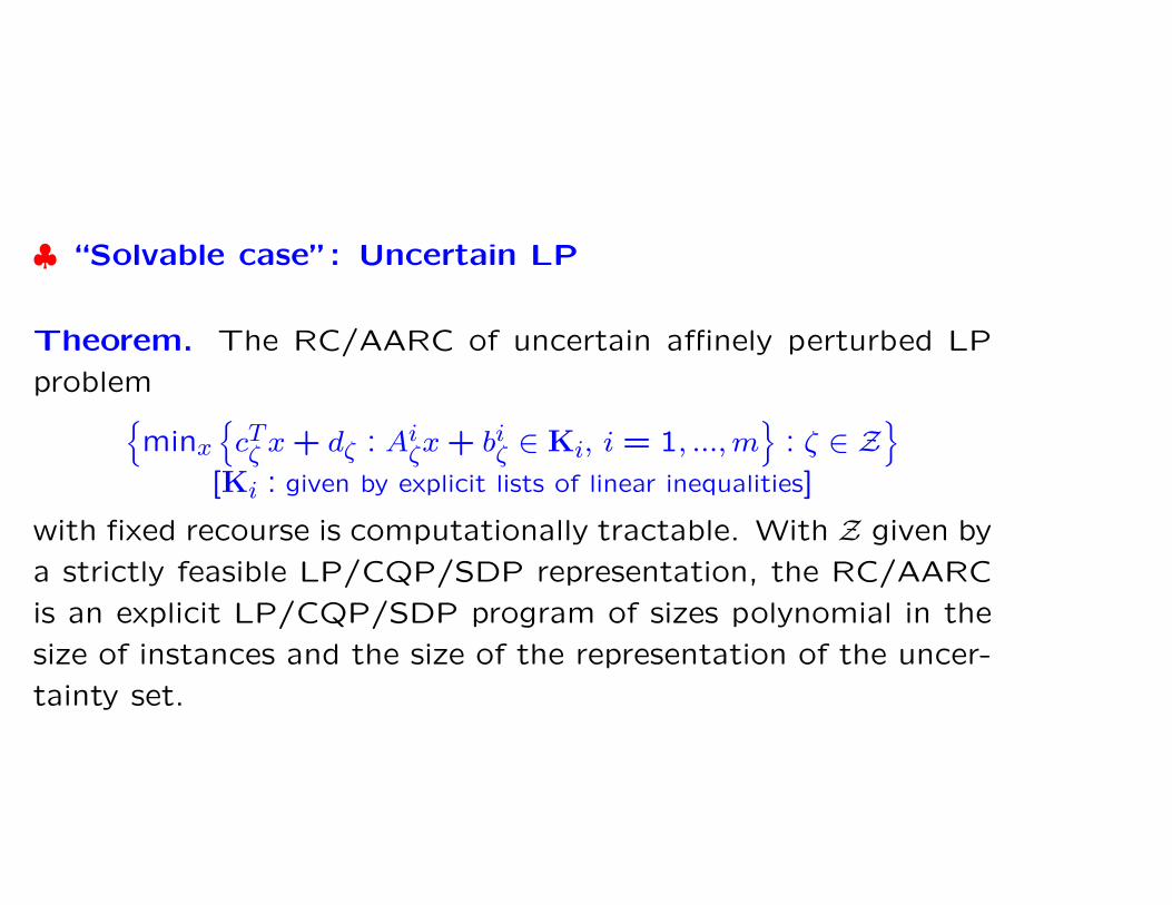
♣ “Solvable case”: Uncertain LP
Theorem. The RC/AARC of uncertain affinely perturbed LP
problem{
minx
{
cTζ x + dζ : Ai
ζx + biζ ∈ Ki, i = 1, ..., m
}
: ζ ∈ Z}
[Ki : given by explicit lists of linear inequalities]
with fixed recourse is computationally tractable. With Z given by
a strictly feasible LP/CQP/SDP representation, the RC/AARC
is an explicit LP/CQP/SDP program of sizes polynomial in the
size of instances and the size of the representation of the uncer-
tainty set.

♣ Aside of a number of highly specific particular cases, semi-
infinite conic quadratic/linear matrix inequalities are computa-
tionally intractable. Whenever it is the case, a natural course
of actions in the RO context is to replace an intractable semi-
infinite conic inequality with its safe tractable approximation.
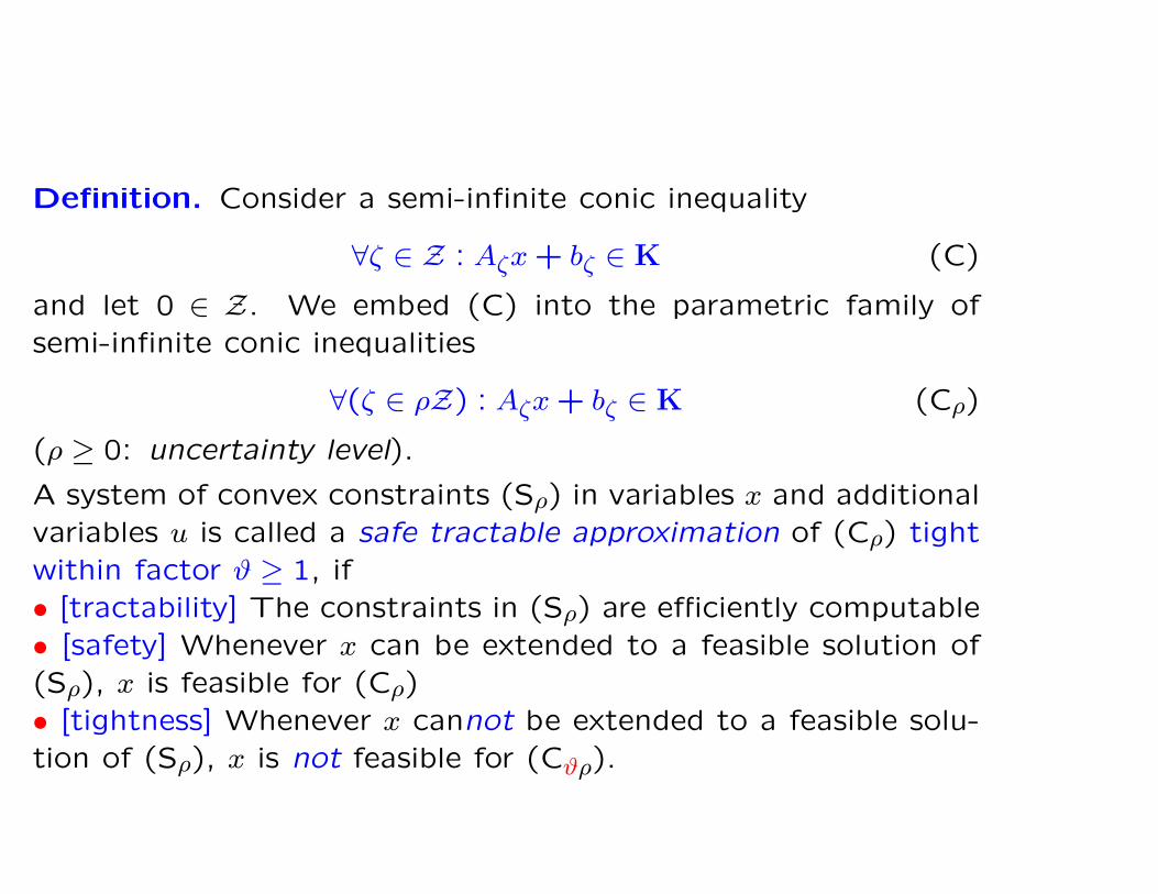
Definition. Consider a semi-infinite conic inequality
∀ζ ∈ Z : Aζx + bζ ∈ K (C)
and let 0 ∈ Z. We embed (C) into the parametric family of
semi-infinite conic inequalities
∀(ζ ∈ ρZ) : Aζx + bζ ∈ K (Cρ)
(ρ ≥ 0: uncertainty level).
A system of convex constraints (Sρ) in variables x and additional
variables u is called a safe tractable approximation of (Cρ) tight
within factor ϑ ≥ 1, if
• [tractability] The constraints in (Sρ) are efficiently computable
• [safety] Whenever x can be extended to a feasible solution of
(Sρ), x is feasible for (Cρ)
• [tightness] Whenever x cannot be extended to a feasible solu-
tion of (Sρ), x is not feasible for (Cϑρ).

♣ Safe tractable approximation of semi-infinite Conic Qu-
adratic Inequality
∀ζ = [ζ`; ζr] ∈ ρZ : ‖Aζ`x − bζ`‖2 ≤ cTζrx − dζr
[
Aζ`, bζ`, cζr, dζr are affine in ζ] (Cρ)
♠ (Cρ) is computationally tractable when:
• [simple ellipsoidal uncertainty] Z is an ellipsoid centered at the
origin
• [side-wise uncertainty with unstructured norm-bounded lhs per-
turbations] Z = Z` ×Zr, Z` = {ζ` ∈ Rp×q : ‖ζ`‖ ≤ 1} and
Aζ`x − bζ` ≡ P (x) + LT (x)ζ`R(x),
where P (x), L(x), R(x) are affine in x and either L(·), or R(·)are constant.

Example: The semi-infinite Least Squares inequality
∀(ζ ∈ Rp×q, ‖ζ‖ ≤ ρ) : ‖
[
[An, bn] + LT ζR]
[x; 1]‖2 ≤ t (Cρ)
admits exact SDP representation
tI − λLTL Anx + bn
λI ρR[x; 1]
[Anx + bn]T ρ[R[x; 1]]T t
� 0 (Sρ)
in variables t, x, λ: (t, x) is feasible for (Cρ) iff it can be extended
to a feasible solution to (Sρ).
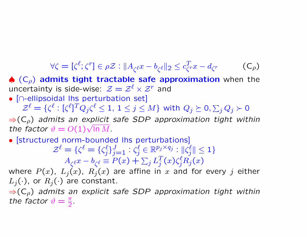
∀ζ = [ζ`; ζr] ∈ ρZ : ‖Aζ`x − bζ`‖2 ≤ cTζrx − dζr (Cρ)
♠ (Cρ) admits tight tractable safe approximation when the
uncertainty is side-wise: Z = Z` ×Zr and
• [∩-ellipsoidal lhs perturbation set]
Z` = {ζ` : [ζ`]TQjζ` ≤ 1, 1 ≤ j ≤ M} with Qj � 0,
∑
j Qj � 0
⇒(Cρ) admits an explicit safe SDP approximation tight within
the factor ϑ = O(1)√
lnM .
• [structured norm-bounded lhs perturbations]
Z` = {ζ` = {ζ`j}J
j=1 : ζ`j ∈ R
pj×qj : ‖ζ`j‖ ≤ 1}
Aζ`x − bζ` ≡ P (x) +∑
j LTj (x)ζ`
jRj(x)
where P (x), Lj(x), Rj(x) are affine in x and for every j either
Lj(·), or Rj(·) are constant.
⇒(Cρ) admits an explicit safe SDP approximation tight within
the factor ϑ = π2.
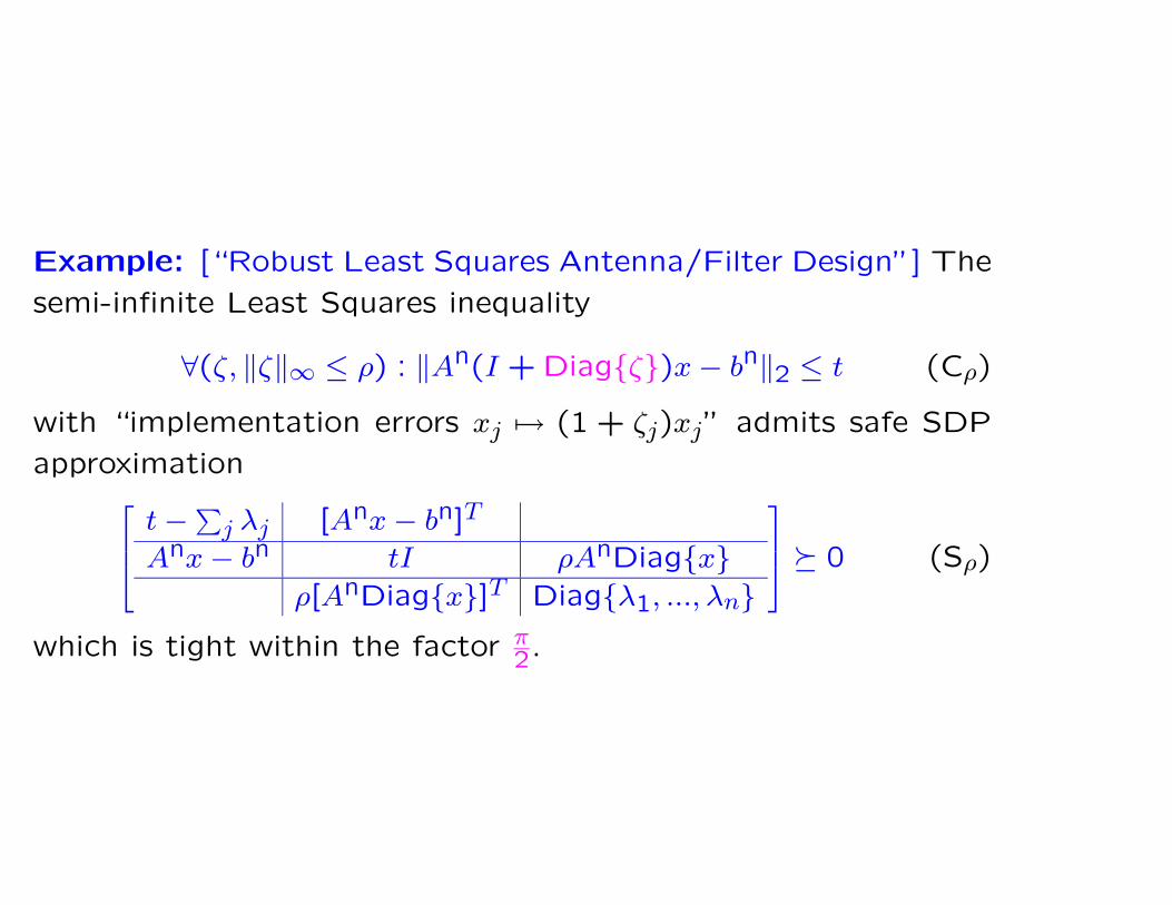
Example: [“Robust Least Squares Antenna/Filter Design”] The
semi-infinite Least Squares inequality
∀(ζ, ‖ζ‖∞ ≤ ρ) : ‖An(I + Diag{ζ})x − bn‖2 ≤ t (Cρ)
with “implementation errors xj 7→ (1 + ζj)xj” admits safe SDP
approximation
t − ∑
j λj [Anx − bn]T
Anx − bn tI ρAnDiag{x}ρ[AnDiag{x}]T Diag{λ1, ..., λn}
� 0 (Sρ)
which is tight within the factor π2.

♣ Safe tractable approximation of semi-infinite Linear Ma-
trix Inequality
∀(ζ ∈ ρZ) : Aζ(x) � 0[
Aζ(x) : bi-affine in x, ζ] (Cρ)
♠ Aside of scenario-generated uncertainty set, the only known
case when (Cρ) admits a tight tractable approximation is the
case of structured norm-bounded uncertainty:
Z = {ζ = {ζj}Mj=1 : ζj ∈ R
pj×pj , ‖ζj‖ ≤ 1, ζj = ξjI, j ∈ J}Aζ(x) = An(x) +
∑
j
[
LTj ζjRj(x) + RT
j (x)ζTj Lj
]
[
An(x),Rj(x) are affine in x]

Theorem. The semi-infinite LMI
∀(
{ζj}Mj=1‖ζj‖ ≤ ρ ∀j, ζj = ξjIpj , j ∈ J
)
:
An(x) +∑
j
[
LTj ζjRj(x) + RT
j (x)ζTj Lj
]
� 0(Cρ)
with structured norm-bounded uncertainty admits a safe tractable
SDP approximation. The tightness factor ϑ of this approxima-
tion depends solely on the largest size of the scalar perturbation
blocks
µ =
{
1, J = ∅maxj∈J pj, J 6= ∅
and does not exceed ϑ(µ), where ϑ(·) is a universal function such
that ϑ(1) = π2, ϑ(2) = 2, ϑ(k) ≤ π
√k. In the case of M = 1 (single
perturbation block), the approximation is exact: ϑ = 1.
Applications in: Robust Structural Design, Lyapunov Stability
Analysis/Synthesis under interval uncertainty, etc.

• Optimization programs with uncertain data and theirRobust Counterparts
• Tractability of Robust Counterparts• Robust Optimization and Chance Constraints
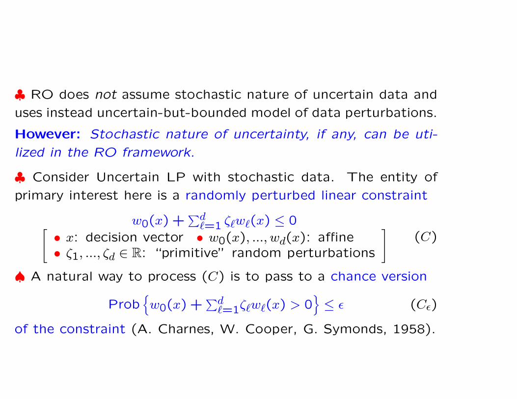
♣ RO does not assume stochastic nature of uncertain data and
uses instead uncertain-but-bounded model of data perturbations.
However: Stochastic nature of uncertainty, if any, can be uti-
lized in the RO framework.
♣ Consider Uncertain LP with stochastic data. The entity of
primary interest here is a randomly perturbed linear constraint
w0(x) +∑d
`=1 ζ`w`(x) ≤ 0[
• x: decision vector • w0(x), ..., wd(x): affine• ζ1, ..., ζd ∈ R: “primitive” random perturbations
]
(C)
♠ A natural way to process (C) is to pass to a chance version
Prob{
w0(x) +∑d
`=1ζ`w`(x) > 0}
≤ ε (Cε)
of the constraint (A. Charnes, W. Cooper, G. Symonds, 1958).
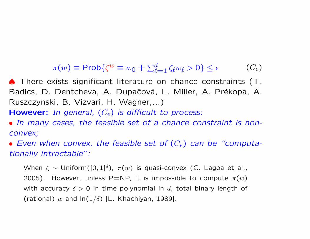
π(w) ≡ Prob{ζw ≡ w0 +∑d
`=1 ζ`w` > 0} ≤ ε (Cε)
♠ There exists significant literature on chance constraints (T.
Badics, D. Dentcheva, A. Dupacova, L. Miller, A. Prekopa, A.
Ruszczynski, B. Vizvari, H. Wagner,...)
However: In general, (Cε) is difficult to process:
• In many cases, the feasible set of a chance constraint is non-
convex;
• Even when convex, the feasible set of (Cε) can be “computa-
tionally intractable”:
When ζ ∼ Uniform([0,1]d), π(w) is quasi-convex (C. Lagoa et al.,
2005). However, unless P=NP, it is impossible to compute π(w)
with accuracy δ > 0 in time polynomial in d, total binary length of
(rational) w and ln(1/δ) [L. Khachiyan, 1989].

π(w) ≡ Prob{ζw ≡ w0 +∑d
`=1 ζ`w` > 0} ≤ ε (Cε)
♣ When (Cε) “as it is” is difficult to process, one can look
for a safe tractable approximation of (Cε) – a computationally
tractable convex set Wε such that
Wε ⊂ {w : π(w) ≤ ε} (∗)♠ A way to build a safe tractable approximation of (Cε):
Take a convex function γ : R → R with lims→−∞
γ(s) = 0,
γ(0) = 1 and set Γ(w) = E {γ(ζw)} .Note: π(w) ≤ Γ(αw) ∀α > 0 and Γ(·) is convex, whence
the set Wε = cl {w : ∃α > 0 : Γ(αw) ≤ ε} is convex and
satisfies (∗).
⇒Whenever Γ(·) is efficiently computable, Wε is a safe tractable
approximation of (Cε).

γ(·) : R → R+, γ(0) = 1 : convex, lims→−∞
γ(s) = 0
⇒ Γ(w) ≥ E
{
γ(
w0 +∑d
`=1 ζ`w`
)}
: convex
⇒ Wε ≡ cl {w : ∃α > 0 : Γ(αw) ≤ ε}⊂{w : Prob{ζw > 0} ≤ ε}Note: Wε is a closed convex cone such that
Wε = {w ∈ Rd+1 : w0 +
∑d
`=1ζ`w` ≤ 0 ∀ζ ∈ Zε}
for an appropriate convex compact set Zε.
⇒The safe approximation w(x) ∈ Wε of the chance constraint
Prob{w0(x) +∑d
`=1 ζ`w`(x) > 0} ≤ ε
is nothing but the Robust Counterpart
∀ζ ∈ Zε : w0(x) + ζ1w1(x) + ... + ζdwd(x) ≤ 0
of the uncertain affinely perturbed linear constraint
w0(x) + ζ1w1(x) + ... + ζdwd(x) ≤ 0
with properly defined perturbation set Zε.

♣ How to choose γ(·)?♠ As far as the conservatism of the upper bound
Prob{ζw > 0} ≤ infα>0
E{γ(ζαw)}[γ(·) ≥ 0 : convex nondecreasing, γ(0) = 1]
is concerned, the best choice of γ(·) is γ(s) = max[1 + s,0].
This choice leads to the famous Conditional Value at Risk safe
approximation
minβ∈R
[
β +1
εE{[ζw − β]+}
]
︸ ︷︷ ︸
CVaRε(w)
≤ 0
of the chance constraint
Prob{ζw > 0} ≤ ε.
However: Typically, CVaRε(·) is difficult to compute...

♣ Ensuring computability: Bernstein approximation [Pin-
ter, 1989; Nem.&Shapiro, 2005]
Observation: Consider a chance constraint
Prob{w0 +∑d
`=1 ζ`w` > 0} ≤ ε (Cε)
and assume that
• ζ1, ..., ζd are independent
• We are smart enough to build efficiently computable
convex bounds Φ`(r) ≥ ln(
E{erζ`})
on the logarithmic
moment-generating functions of ζ`, ` = 1, ..., d.
Choosing γ(s) = es, one can set
Γ(w) = exp{w0 +∑d
`=1 Φ`(w`)}thus arriving at a tractable safe approximation of (Cε).

Example (one of many): Range and mean a priori information
on ζ`. Consider a chance constraint
Prob{w0(x) +∑d
`=1 ζ`w`(x) > 0} ≤ ε
• ζ` ∈ [−1,1]: independent • E{ζ`} ∈ [µ−` , µ+
` ](Cε)
The associated Bernstein approximation of (Cε) is
∀ζ ∈ Zε : w0(x) +∑d
`=1 ζ`w`(x) ≤ 0,
Zε = {ζ :∑d
`=1 φ`(ζ`) ≤ 2 ln(1/ε)}
φ`(s) =
(1 + s) ln(
1+s1+µ−
`
)
+ (1 − s) ln(
1−s1−µ−
`
)
,−1 ≤ s ≤ µ−`
0 , µ−` ≤ s ≤ µ+
`
(1 + s) ln(
1+s1+µ+
`
)
+ (1 − s) ln(
1−s1−µ+
`
)
, µ+` ≤ s ≤ 1
(Br)
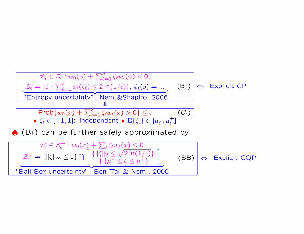
∀ζ ∈ Zε : w0(x) +∑d
`=1 ζ`w`(x) ≤ 0,
Zε = {ζ :∑d
`=1 φ`(ζ`) ≤ 2 ln(1/ε)}, φ`(s) = ...︸ ︷︷ ︸
“Entropy uncertainty”, Nem.&Shapiro, 2006
(Br) ⇔ Explicit CP
⇓Prob{w0(x) +
∑d`=1 ζ`w`(x) > 0} ≤ ε (Cε)
• ζ` ∈ [−1,1]: independent • E{ζ`} ∈ [µ−` , µ+
` ]
♠ (Br) can be further safely approximated by
∀ζ ∈ Z+ε : w0(x) +
∑
` ζ`w`(x) ≤ 0
Z+ε = {‖ζ‖∞ ≤ 1}⋂
[
{‖ζ‖2 ≤√
2 ln(1/ε)}+{µ− ≤ ζ ≤ µ+}
]
︸ ︷︷ ︸
“Ball-Box uncertainty”, Ben-Tal & Nem., 2000
(BB) ⇔ Explicit CQP

∀ζ ∈ Z+ε : w0(x) +
∑
` ζ`w`(x) ≤ 0
Z+ε = {‖ζ‖∞ ≤ 1}⋂
[
{‖ζ‖2 ≤√
2 ln(1/ε)}+{µ− ≤ ζ ≤ µ+}
](BB) ⇔ Explicit CQP
⇓∀ζ ∈ Zε : w0(x) +
∑d`=1 ζ`w`(x) ≤ 0,
Zε = {ζ :∑d
`=1 φ`(ζ`) ≤ 2 ln(1/ε)}, φ`(s) = ...(Br) ⇔ Explicit CP
⇓Prob{w0(x) +
∑d`=1 ζ`w`(x) > 0} ≤ ε (Cε)
• ζ` ∈ [−1,1]: independent • E{ζ`} ∈ [µ−` , µ+
` ]
♠ (BB) is further safely approximated by
∀ζ ∈ Z++ε : w0(x) +
∑
` ζ`w`(x) ≤ 0
Z++ε = {‖ζ‖∞ ≤ 1}
⋂[
{‖ζ‖1 ≤√
2d ln(1/ε)}+{µ− ≤ ζ ≤ µ+}
]
︸ ︷︷ ︸
“Budgeted uncertainty”, Bertsimas & Sim, 2003
(Bd) ⇔ Explicit LP

∀ζ ∈ Z : w0(x) +∑d
`=1 ζ`w`(x) ≤ 0 (RC[Z])⇓
Prob{w0(x) +∑d
`=1 ζ`w`(x) > 0} ≤ ε (Cε)
• ζ` ∈ [−1,1]: independent • E{ζ`} ∈ [µ−` , µ+
` ]
d = 64 d = 128 d = 256
Random 2D cross-sections of Entropy (red), Ball-Box (yellow)
and Budgeted (green) uncertainty sets, ε = 0.005, µ±` = 0.
Black: cross-section of the support {‖ζ‖∞ ≤ 1} of ζ.
Recommended


![Selected topics in robust convex optimizationnemirovs/MP_SelectedRO_2008.pdfSelected topics in robust convex optimization 127 Signal processing and estimation [4,29,33].1 It would](https://img.pdfslide.us/doc/110x75/603e905b21cf823451262378/selected-topics-in-robust-convex-nemirovsmpselectedro2008pdf-selected-topics.jpg)