Robust Optimization and Data Approximation in
Machine Learning
Gia Vinh Anh Pham
Electrical Engineering and Computer SciencesUniversity of California at Berkeley
Technical Report No. UCB/EECS-2015-216
http://www.eecs.berkeley.edu/Pubs/TechRpts/2015/EECS-2015-216.html
December 1, 2015

Copyright © 2015, by the author(s).All rights reserved.
Permission to make digital or hard copies of all or part of this work forpersonal or classroom use is granted without fee provided that copies arenot made or distributed for profit or commercial advantage and that copiesbear this notice and the full citation on the first page. To copy otherwise, torepublish, to post on servers or to redistribute to lists, requires prior specificpermission.
Robust Optimization and Data Approximation in Machine Learning
by
Gia Vinh Anh Pham
A dissertation submitted in partial satisfactionof the requirements for the degree of
Doctor of Philosophy
in
Computer Science
in the
GRADUATE DIVISION
of the
UNIVERSITY OF CALIFORNIA, BERKELEY
Committee in charge:
Professor Laurent El Ghaoui, ChairProfessor Bin Yu
Professor Ming Gu

The dissertation of Gia Vinh Anh Pham is approved.
Chair Date
Date
Date
University of California, Berkeley

Robust Optimization and Data Approximation in Machine Learning
Copyright c©
by
Gia Vinh Anh Pham
Abstract
Robust Optimization and Data Approximation in Machine Learning
by
Gia Vinh Anh Pham
Doctor of Philosophy in Computer Science
University of California, Berkeley
Professor Laurent El Ghaoui, Chair
Modern learning problems in nature language processing, computer vision, computational
biology, etc. often involve large-scale datasets with millions of samples and/or millions of
features, thus are challenging to solve. Simply replacing the original data with a simpler
approximation such as a sparse matrix or a low-rank matrix does allow a dramatic reduction
in the computational effort required to solve the problem, however some information of
the original data will be lost during the approximation process. In some cases, the solution
obtained by directly solving the learning problem with approximated data might be infeasible
for the original problem or might have undesired properties. In this thesis, we present a new
approach that utilizes data approximation techniques and takes into account, via robust
optimization the error made during the approximation process in order to obtain learning
algorithms that could solve large-scale learning problems efficiently while preserving the
learning quality.
In the first part of this thesis, we give a brief review of robust optimization
and its appearance in machine learning literature. In the second part of this the-
1

sis, we examine two data approximation techniques, namely data thresholding and
low-rank approximation, and then discuss their connection to robust optimization.
Professor Laurent El GhaouiDissertation Committee Chair
2

Dedicated to my parents, Cuong Pham & Nguyet Nguyen, and my wife Dan-Quynh Tran
for their continuous support and encouragement throughout my life.
i
Contents
Contents ii
Acknowledgements vi
1 Introduction 1
2 Robust Optimization 3
2.1 General optimization problem . . . . . . . . . . . . . . . . . . . . . . . . . . 3
2.2 Robust optimization and Data uncertainty . . . . . . . . . . . . . . . . . . . 6
2.2.1 Robust optimization vs. Sensitivity analysis . . . . . . . . . . . . . . 7
2.2.2 Robust optimization vs. Stochastic optimization . . . . . . . . . . . . 7
2.2.3 Example: linear programming problem . . . . . . . . . . . . . . . . . 8
2.3 Robust optimization in Machine learning . . . . . . . . . . . . . . . . . . . . 11
2.3.1 Data uncertainty models . . . . . . . . . . . . . . . . . . . . . . . . . 11
2.3.2 Connection to regularization . . . . . . . . . . . . . . . . . . . . . . . 13
2.4 Robust optimization and Data approximation . . . . . . . . . . . . . . . . . 15
2.4.1 Data approximation . . . . . . . . . . . . . . . . . . . . . . . . . . . 15
2.4.2 Is data approximation enough? . . . . . . . . . . . . . . . . . . . . . 17
3 Data Thresholding 19
3.1 Introduction . . . . . . . . . . . . . . . . . . . . . . . . . . . . . . . . . . . . 19
3.2 Data thresholding for sparse linear classification problems . . . . . . . . . . . 21
ii
3.2.1 Penalized problem . . . . . . . . . . . . . . . . . . . . . . . . . . . . 22
3.2.2 Constrained problem . . . . . . . . . . . . . . . . . . . . . . . . . . . 24
3.2.3 Iterative thresholding . . . . . . . . . . . . . . . . . . . . . . . . . . . 26
3.3 Experimental results . . . . . . . . . . . . . . . . . . . . . . . . . . . . . . . 26
3.3.1 UCI Forest Covertype dataset . . . . . . . . . . . . . . . . . . . . . . 27
3.3.2 20 Newsgroup Dataset . . . . . . . . . . . . . . . . . . . . . . . . . . 28
3.3.3 UCI NYTimes dataset . . . . . . . . . . . . . . . . . . . . . . . . . . 29
4 Low-rank Approximation 31
4.1 Introduction . . . . . . . . . . . . . . . . . . . . . . . . . . . . . . . . . . . . 31
4.2 Algorithms for Low-rank Approximation . . . . . . . . . . . . . . . . . . . . 33
4.2.1 First order methods with Low-rank approximation . . . . . . . . . . . 34
4.3 Robust Low-rank LASSO . . . . . . . . . . . . . . . . . . . . . . . . . . . . 37
4.3.1 Theoretical Analysis . . . . . . . . . . . . . . . . . . . . . . . . . . . 40
4.3.2 Discussion . . . . . . . . . . . . . . . . . . . . . . . . . . . . . . . . . 43
4.3.3 Regularized Robust Rank-1 LASSO . . . . . . . . . . . . . . . . . . . 45
4.4 Experimental Results . . . . . . . . . . . . . . . . . . . . . . . . . . . . . . . 47
4.4.1 Datasets . . . . . . . . . . . . . . . . . . . . . . . . . . . . . . . . . . 48
4.4.2 Multi-label classification . . . . . . . . . . . . . . . . . . . . . . . . . 49
4.4.3 When labels are columns of data matrix . . . . . . . . . . . . . . . . 50
5 Conclusion 54
Bibliography 56
iii
List of Figures
3.1 Result of SVM with data thresholding on UCI Forest Covertype dataset. . . 27
3.2 Speed-up and space-saving for SVM with data thresholding on 20 Newsgroup
dataset, topic = comp.graphics. Number of training samples: 13K, number
of features: 61K. . . . . . . . . . . . . . . . . . . . . . . . . . . . . . . . . . 29
4.1 Rank-1 LASSO (left) and Robust Rank-1 LASSO (right) with random data.
The plot shows the elements of the optimizer as a function of the l1-norm
penalty parameter λ. The non-robust solution has cardinality 1 or 0 for all
of 0 < λ < C for some C. The robust version allows a much better control of
the sparsity of the solution as a function of λ. . . . . . . . . . . . . . . . . . 44
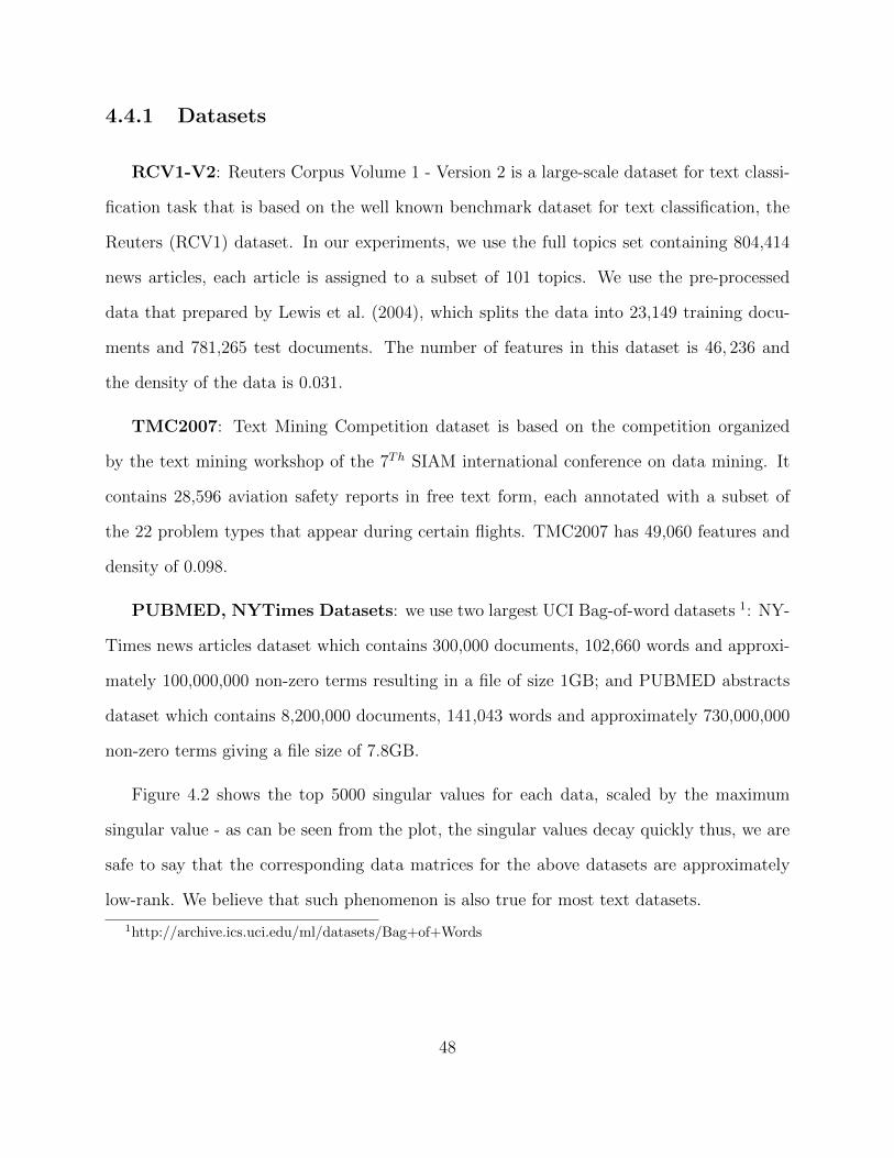
4.2 Top 5000 singular values for each dataset, scaled by maximum singular value.
The size of each dataset (number of samples x number of features) is also shown. 49
4.3 Multi-label classification: RCV1V2 dataset . . . . . . . . . . . . . . . . . . . 50
4.4 Multi-label classification: TMC2007 dataset . . . . . . . . . . . . . . . . . . 51
iv
List of Tables
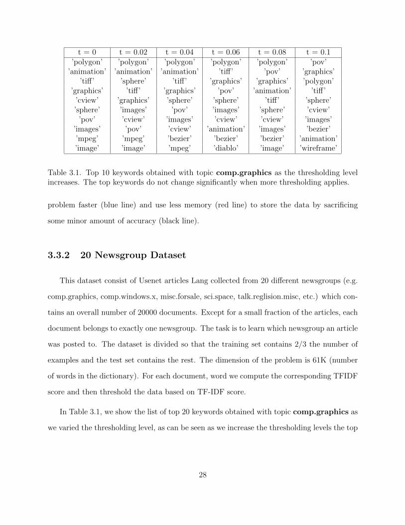
3.1 Top 10 keywords obtained with topic comp.graphics as the thresholding
level increases. The top keywords do not change significantly when more
thresholding applies. . . . . . . . . . . . . . . . . . . . . . . . . . . . . . . . 28
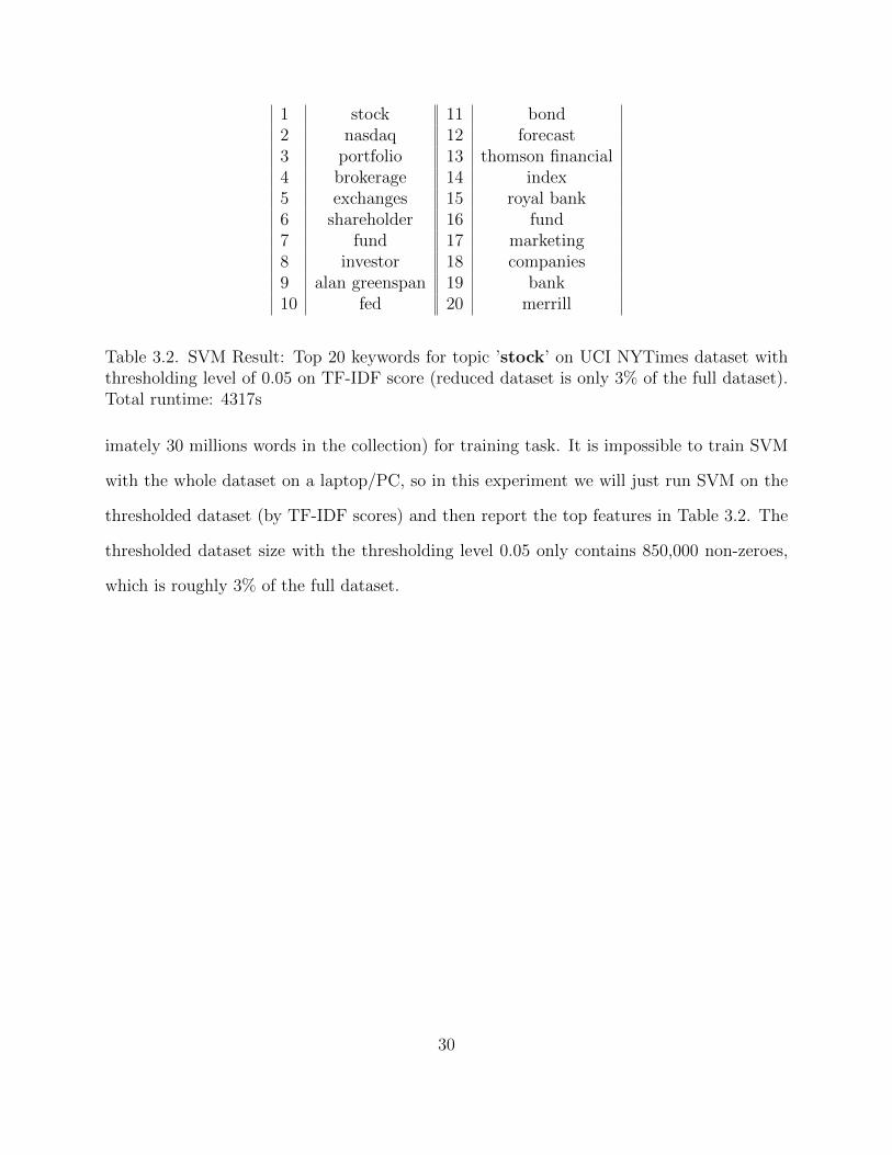
3.2 SVM Result: Top 20 keywords for topic ’stock’ on UCI NYTimes dataset
with thresholding level of 0.05 on TF-IDF score (reduced dataset is only 3%
of the full dataset). Total runtime: 4317s . . . . . . . . . . . . . . . . . . . . 30
4.1 NYTimes news articles - top 10 predictive words for different query terms
(10 industry sectors). Low-rank approximation with k = 20 is used, total
training time (for all query terms) is 42918 seconds . . . . . . . . . . . . . . 52
4.2 PUBMED abstracts - top 10 predictive words for different query terms (10
diseases). Low-rank approximation with k = 20 is used, total training time
(for all query terms) is 56352 seconds . . . . . . . . . . . . . . . . . . . . . . 53
v

Acknowledgements
First, I would like to thank my parents, my wife and my brother for their unconditional love
and constant support. They have been the source of motivation for me to get through the
ups and downs of graduate student’s life.
With profound gratitude, I want to thank my advisor, Professor Laurent El Ghaoui for
tolerating my ignorance during my time at Berkeley and encouraging me when I was at my
most difficult moments. I have grown significantly since I met Laurent, both personally and
academically, and I am extremely grateful for his guidance.
I would like to thank Professor Bin Yu and Professor Ming Gu for being on my thesis
committee and for their valuable feedbacks and suggestions during my qualification exam.
Finally I want to thank my colleagues and friends at Berkeley, who have provided count-
less technical, intellectual, and personal help with various aspects of my work. These include,
but are not limited to, Tarek Rabbani, Youwei Zhang, Andrew Godbehere, Mert Pilanci and
other members past and present of StatNews group for their help and support.
vi

vii

Chapter 1
Introduction
Modern supervised learning algorithms such as support vector machine or logistic regres-
sion have become popular tools and widely used in many areas: natural language processing,
computer vision, data mining, bioinformatics, etc.. In most of real-world learning problems,
for instance text classification, the number of features can be very large - hundreds of thou-
sands or millions, so is the number of training samples; thus, we have to face the daunting
task of storing and operating on matrices with thousands to millions rows and columns. It
is expensive to store the large-scale data in the memory and in many cases the data cannot
even be loaded into the memory. More importantly, these learning algorithms often require
us to solve a large convex optimization problem in which under large-scale setting, might be
impossible at times.
In many machine learning applications, the problem data involved is closed to one having
a simple structure (we will see in more details in Chapter 3 and 4), for example the input
data could be closed to a sparse matrix or a low-rank matrix, etc.. If the data matrix has
exactly simple structure then it is often possible to exploit that structure to decrease the
1

computational time and the memory needed to solve the problem. What if, instead, the data
matrix is only approximately simple, and we have at our disposal the simple approximation?
In this dissertation, we will introduce a new approach that uses data approximation
under robust optimization scheme to deal with large-scale learning problems. The main idea
is that instead of ignoring the error made by approximating the original data with a simpler
structure, we consider such error as some sort of artificially introduced data uncertainty 1
and then use robust optimization to obtain modified learning algorithms that are capable
of handling the approximation error even in worst case scenario. We show that the savings
obtained using data approximation still hold for the robust counterpart problem1. In this
sense, our approach takes advantage of the simpler problem structure on the computational
level; in addition it allows to control the noise. The proposed approach has both advantage of
having memory saving and computational speedups as well as having reliable performance.
The thesis is organized as follows: we first describe robust optimization and its important
concepts such as data uncertainty and robust counterpart problem in Chapter 2. We will
also briefly review robust optimization in machine learning literature in Chapter 2. We then
introduce data thresholding technique for large-scale sparse linear classification in Chapter 3.
In Chapter 4, we will introduce an efficient and scalable robust low-rank model for LASSO
problem. We draw conclusions and point out some future research directions in Chapter 5.
1this concept will be described in details in Chapter 2
2
Chapter 2
Robust Optimization
2.1 General optimization problem
In general mathematical optimization, we often assume that the input data is precisely
known, and we seek to optimize an objective function over a set of decision variables as
following:
minx
f0(x, u0)
subject to fi(x, ui) ≤ 0, i = 1, . . . ,m(2.1.1)
where x ∈ Rd is a vector of decision variables and uimi=1 are known input parameters for
functions fimi=1.
Many machine learning problems require us to solve an optimization problem - usually
a convex optimization problem of the form (2.1.1). Following are some of such problems in
which we will look at in the latter chapters of this thesis:
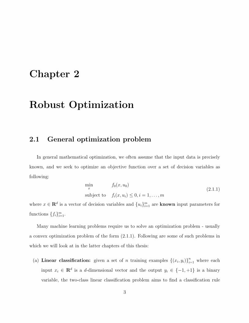
(a) Linear classification: given a set of n training examples (xi, yi)ni=1 where each
input xi ∈ Rd is a d-dimensional vector and the output yi ∈ −1,+1 is a binary
variable, the two-class linear classification problem aims to find a classification rule
3
from training data so that given new input x ∈ Rd, we can “optimally” assign a class
label y ∈ −1,+1 to x, for example y = sign(wTx+b) for some weight vector w ∈ Rd
and scalar b ∈ R. In general, the linear classification problem seeks for the optimal
solution of the following optimization problem:
minw∈Rd,b∈R
1
n
n∑i=1
f(yi(w
Txi + b))
+R(w)
where f : R → R+ is a non-negative convex function, so called the loss function and
R : Rd → R+ is the regularization function.
• In case of Support Vector Machines (SVM), the loss functions is hinge loss:
f(z) = [1− z]+ (we define [z]+ := max(0, z))
minw∈Rd,b∈R
1
n
n∑i=1
[1− (yi(wTxi + b)]+ +R(w)
• For logistic regression, the loss function is logistic loss: f(z) = log(1 + e−z).
minw∈Rd,b∈R
1
n
n∑i=1
log(1 + exp(−yi(wTxi + b))
)+R(w)
The regularization term is widely used to seeks a trade-off between fitting the observa-
tions and reducing the model complexity, for example: l1-regularization R(w) = λ‖w‖1,
or l2-regularization R(w) = λ‖w‖2.
(b) Least squares regression and its variations: given a response vector y ∈ Rn and
data matrix X ∈ Rd×n (each column of X corresponds to a data sample in Rd), the
least squares regression problem is to find a weight vector w ∈ Rd so that the l2 norm
of the residual y−XTw is minimized, i.e. solving the following optimization problem:
minw‖y −XTw‖2
Since minimizing the squared error can lead to sensitive solutions (Golub and Van Loan
(1996)), variations of least squares problem that use regularization methods such as
4
Tikhonov regularization (Tikhonov and Arsenin (1977)) - using l2 norm regularization,
and LASSO - Least Absolute Shrinkage and Selection Operator (Tibshirani (1996);
Efron et al. (2004)) - using l1 norm regularization. Both methods provide some level
of regularity to the solution. LASSO is also known for selecting sparse solutions, i.e.
having few entries that are non-zero, and therefore identifying the features on the data
matrix X that are useful to predict the response vector y.
(c) More general supervised learning problems: linear classification and regression
problems, amongst many others, can be generalized to solving the following optimiza-
tion problem:
minv∈R,w∈C
f(ATw + cv) (2.1.2)
where the loss function f : Rn → R+ is convex, the data matrix A ∈ Rd×n and vector
c ∈ Rn are given, C ⊆ Rd is a convex set that constraining the decision variable w.
This formulation covers well-known problems, for example:
• By choosing f(z) :=∑n
i=1(1 − zi)+, A := [y1x1, . . . , ynxn], c := y, v := b and
the constraint set C := w : ‖w‖2 ≤ λ we obtained the (constrained) l2-SVM
problem:
min‖β‖2≤λ
n∑i=1
[1− yi(xTi w + b)]+
• By choosing f(z) := ‖y − z‖2, c := 0, A := [x1, . . . , xn] and the constrain set
C := w ∈ Rd : ‖w‖1 ≤ λ we obtained the LASSO problem:
min‖w‖1≤λ
‖y −XTw‖2
5
2.2 Robust optimization and Data uncertainty
When a real-world application is formulated as a mathematical optimization problem,
more often than not the problem data is not precisely known, but is subject to some sort of
uncertainty due to many factors - for example:
• prediction errors : occur when we do not have the data at the time the problem is
solved and we need to predict their values.
• measurement errors : occur when we cannot record the data exactly due to limitation
of measurement devices.
The data uncertainty can affect either the feasibility of a solution to the optimization
problem, or it could affect the optimality of a solution, or both. Robust optimization pro-
vides a novel and systematic approach to deal with problems involving data uncertainty by
generating a robust solution that is immunized against the effect of data uncertainty.
When data uncertainty affects the feasibility of a solution (i.e. the constraints), robust
optimization seeks to obtain a solution that is feasible for any possible realization of the
unknown parameters; and when data uncertainty affects the optimality of a solution (i.e.
the objective function), robust optimization seeks to obtain a solution that optimizes the
worst case scenario. In particular, suppose that the parameters u = (u0, . . . , um) varies
in some uncertainty set U that characterizes the unknown parameters u, the robust
counterpart problem solves:
minx
maxu∈U
f0(x, u0)
subject to ∀u ∈ U : fi(x, ui) ≤ 0, i = 1, . . . ,m.(2.2.1)
6
The goal of (2.2.1) is to compute the optimal solution that minimizes the worst case
objective function amongst all those solutions which are feasible for all realizations of the
disturbances that affects the parameters u within the uncertainty set U .
Being a conservative (worst-case oriented) methodology, robust optimization is often
useful when the optimization problems have hard constraints that must be satisfied no matter
what, or the objective function/optimal solutions are highly sensitive to perturbations, or we
cannot afford low probability high-magnitude risks (for example in aerospace design, nuclear
plant design, etc.).
2.2.1 Robust optimization vs. Sensitivity analysis
Sensitivity analysis is another traditional method of dealing with data uncertainty. How-
ever, unlike robust optimization that seeks for an uncertainty-immunized solution under
worst-case scenario to an optimization problem involving uncertainty data, sensitivity anal-
ysis aims at analyzing the goodness of a solution when there are small perturbations in the
underlying problem data. It first solves the problem with fixed values of the parameters
and then see how the optimal solution is affected by small perturbations. Such post-mortem
analysis is not helpful for computing the solutions that are robust to data perturbation.
2.2.2 Robust optimization vs. Stochastic optimization
In stochastic optimization, the data uncertainty are assumed to be random and the
feasibility of a solution is expressed using chance constraints. Suppose that we know in
advance the distribution of the input parameters, the corresponding stochastic optimization
7

is:
minx
t
subject to Pu0∼P0 [f0(x, u0) ≤ t] ≥ 1− ε0,
and Pui∼Pi[fi(x, ui) ≤ 0] ≥ 1− εi, i = 1, . . . ,m
(2.2.2)
where εi 1, i = 0, . . . ,m are given tolerances and Pi is the distribution of the input
parameter ui, i = 0, . . . ,m.
Although the above model (2.2.2) is powerful, there are some associated fundamental
difficulties. First of all, it is difficult to obtain the actual distributions of the uncertain input
parameters, and sometimes it is hard to interpret these distributions as well. Furthermore,
even if we can obtain the probabilistic distributions, it is still computationally challenging
to check the feasibility of the chance constraints, even more challenging to solve the opti-
mization problem. In many cases, the chance constraints can destroy convexity and make
the stochastic optimization problem become computationally intractable.
2.2.3 Example: linear programming problem
One could model the uncertainty set as flexibly as he/she wants, either using probablistic
data model or uncertainty-but-bounded data model. To illustrate the concept of robust
optimization and data uncertainty, we consider a simple linear programming problem:
minx∈Rd
cTx
subject to aix ≤ bi, i = 1, . . . , n
Below are some examples of how we could model data uncertainty and how we could
derive the robust counterpart problems:
(a) data uncertainty in objective function
8

Suppose that the cost vector c ∈ Rd is uncertain but lies in a ball centered at a known
vector c ∈ Rd and radius R > 0: B(c, λ) := c : ‖c− c‖2 ≤ R, the robust counterpart
problem writes:
minx
max‖c−c‖2≤R
cTx
subject to aix ≤ bi, i = 1, . . . , n
Since max‖c−c‖2≤R
cTx = cTx+ max‖z‖2≤R
zTx = cTx+R‖x‖2, the robust counterpart problem
is thus:
minx
cTx+R‖x‖2
subject to aix ≤ bi, i = 1, . . . , n
(b) data uncertainty in constraints - decoupled
Suppose that the data uncertainty occurs in the constraints, and the uncertainty for
vectors ai are decoupled, each vector ai could be perturbed in a l2 fixed ball with a
known center and radius : Ui := ai : ai = ai + δi, ‖δi‖2 ≤ Ri, i = 1, . . . , n, the robust
counterpart problem writes:
minx
cTx
subject to (ai + δi)x ≤ bi,∀δi : ‖δi‖2 ≤ Ri, i = 1, . . . , n
Since (ai + δi)Tx ≤ bi, ∀δi : ‖δi‖2 ≤ Ri if and only if max‖δi‖2≤Ri
(ai + δi)Tx ≤ bi , which
is equivalent to aTi x+Ri‖x‖2 ≤ bi, the robust counterpart problem is thus:
minx
cTx
subject to aix+Ri‖x‖2 ≤ bi, i = 1, . . . , n
(c) data uncertainty in constraints - coupled
Suppose that the data uncertainty occurs in the constraints, and the uncertainty for
vectors ai are coupled, given as: U := A : A = A + ∆, ‖∆‖F ≤ R where A ∈ Rn×d
9

is the matrix with rows aini=1. The robust counterpart problem writes:
minx
cTx
subject to (A+ ∆)x ≤ b,∀∆ ∈ Rn×d : ‖∆‖F ≤ R
Since (A + ∆)x ≤ b,∀∆ ∈ Rn×d : ‖∆‖F ≤ R if and only if max‖∆‖F≤R(A + ∆)x ≤ b,
which is equivalent to Ax+R‖x‖21 ≤ b, the robust counterpart problem is thus:
minx
cTx
subject to Ax+R‖x‖21 ≤ b
(d) probabilistic data uncertainty model
For simplicity, we consider the case that n = 1, i.e. A := aT ∈ Rd×1, b ∈ R. Suppose
that our data (a, b) varies in the uncertainty set
U :=
[aδ, bδ] = [a(0), b(0)] +
K∑k=1
δk[a(k), b(k)] : δ ∼ P
where a(k), b(k), k = 0, . . . , K are known and the distribution P is also known. The
robust counterpart problem writes:
minx
cTx
subject to Pδ∼P[aTδ x ≤ bδ
]≥ 1− ε
Dealing with such probabilistic model is difficult, very often the problem is severely
computationally intractable. In few cases, for example when P is Gaussian distribution,
i.e. δ ∼ N (µ,Σ) and ε < 1/2, the problem is tractable. Indeed, we observe that
zx = aTδ x− bδ = [a(0)]Tx+K∑k=1
δk[a(k)]Tx− b(0) −
K∑k=1
δkb(k)
is a Gaussian random variable with the expectation E[zx] = αT [x; 1] and variable
var[zx] = [x; 1]TQTQ[x; 1] where α and Q are vector and matrix that can be computed
from the data [a(k), b(k)], µ,Σ. Via some derivations, noting that ε ∈ [0, 1/2], we
10
can reduce the probabilistic constraint is P[zx ≤ 0] ≥ 1 − ε to the second-order cone
constraint αT [x; 1] + Cε‖Q[x; 1]‖2 ≤ 0 for some constant Cε. The robust counterpart
problem is thus:
minx
cTx
subject to αT [x; 1] + Cε‖Q[x; 1]‖2 ≤ 0
Due to the complexity and intractability of probabilistic data uncertainty model, in
this thesis we will only focus on uncertain-but-bounded models.
2.3 Robust optimization in Machine learning
In recent years, there have been a number of works on the idea of using robust opti-
mization to deal with data uncertainty that arises in many machine learning models. These
works essentially consider learning problems in which training samples are assumed to be
uncertain - but restricted in some bounded sets, and then proposes robustified learning algo-
rithms that are modified versions of the nominal learning algorithms to guarantee immunity
to data pertubations.
2.3.1 Data uncertainty models
Bhattacharyya (2004); Bhattachryya et al. (2003) investigated on linear classification
problem (SVM) assuming an ellipsoidal model of uncertainty in which each data sample xi
is uncertain but lies in a known ellipsoid B(xi,Σi, γi) := x : (x − xi)TΣ−1(x − xi) ≤ γ2i .
The corresponding robustified learning algorithm is then formulated as an SOCP (Second
Order Cone Programming), which can be solved efficiently:
11
minw,b,ξ
n∑i=1
ξi
subject to yi(wTxi + b) ≥ −ξi + γi‖Σ1/2
i w‖2
‖w‖2 ≤ A
ξi ≥ 0,∀i = 1, . . . , n
Trafalis and Gilbert (2007) considered lp-norm uncertainty sets for SVM problem, in
which each data sample xi is assumed to be in an lp-ball Bp(xi, ηi) := x : ‖x− xi‖p ≤ ηi.
The resulting robust counterpart optimization problem can be transformed into an SOCP
when p = 2 and or simply a linear programming problem when p = 1 or p =∞.
Going further, Shivaswamy et al. (2006) considered linear classification and linear regres-
sion problems under probabilistic data uncertain model, assuming that each data sample
xi is a random variable picked from a family of distributions which have a known mean
and covariance. The authors also proposed SOCP formulations that robustify the standard
learning algorithms and showed that these formulations outperform the imputation based
classifiers and regression functions when applying to the missing variable problem.
Globerson and Roweis (2006) introduced a robust optiomization-inspired method for
learning SVM classifiers under a worst case scenario of feature deletion at test time. In
particular, the data uncertainty model assumes that up to K features may be deleted/missing
from each data vector and then compute the worst case objective function. The authors
considered the following nominal problem (bias term is not introduced explicitly, and could
be included by adding a constant feature):
minw
1
2‖w‖2
2 + C
n∑i=1
[1− yiwTxi]+
Under worst case scenario when up to K features may be deleted from each data vector, the
12
worst case hinge loss [1−yowTxi]+ of sample i can be derived to be [1−yiwTxi+si]+, where
si = maxαi∈Rd
yiwT (xi αi)
s.t. 0 ≤ αi ≤ 1∑j αij = K
where denotes point-wise multiplication. The resulting robust counterpart problem can be
written as the following quadratic problem and can be solved efficiently:
minw,t,z,v
1
2‖w‖2
2 + Cn∑i=1
[1− yiwTxi + ti]+
subject to ti ≥ Kzi +∑
j vij
vi ≥ 0
zi + vi ≥ yixi w
Data uncertainty is not only modeled for data points in the feature space but also for
data labels. Caramanis and Mannor (2008) studied two types of adversarial disturbance in
which the labels are corrupted: disturbance in the labels of a certain fraction of the data,
and disturbance that affects the position of the data points. The authors proposed a general
optimization-theoretic algorithmic framework for finding a classifier under these disturbances
and provided distribution-dependent bounds on the amount of error as a function of the noise
level for the two models.
A comprehensive study of other data uncertainty models for machine learning problems
can also be found in (Ben-Tal et al. (2009)).
2.3.2 Connection to regularization
Robust optimization and regularization in machine learning are strongly related, and in
some cases are equivalent. Early work by Ghaoui and Lebret (1997), Anthony and Bartlett
13
(1999) showed that structured robust solutions to least squares problems with uncertain data
under Frobenius norm can be interpreted as a Tikhonov (l2) regularization procedures:
Theorem 1 The following robust optimization formulation of the lease squares problem in
which the data uncertainty set is described by U = U ∈ Rd×n : ‖U‖F ≤ λ:
minβ∈Rd
maxU∈U‖y − (X + U)Tβ‖2
is equivalent to Tikonov-regularized regression problem:
minβ∈Rd
‖y −Xβ‖2 + λ‖β‖2
Recently, Xu et al. (2011) created a precise connection between robustness and regularized
Support Vector Machine via notions of sublinear aggregated uncertainty set, which defined
as follows:
Definition 1 U0 ⊆ Rn is called Atomic Uncertainty Set if
(i) 0 ∈ U0
(ii) ∀w0 ∈ Rn : supu∈U0
wT0 u = supu′∈U0
wT0 u′ < +∞
Definition 2 U ⊆ Rn×m is called Sublinear Aggregated Uncertainty Set of U0, if U− ⊆ U ⊆
U+ where
U− =m⋃k=1
U−k where U−k := (u1, . . . , um)|uk ∈ U0;ui 6=k = 0
U+ =
(α1u1, . . . , αmum)|
m∑i=1
αi = 1, αi ≥ 0, ui ∈ U0, i = 1, . . . ,m
14
Theorem 2 Xu et al. (2011) Assume xi, yini=1 are non-separable and U is a sublinear
aggregated uncertainty set then the following problems are equivalent:
(P1) minw,b
max(u1,...,un)∈U
R(w, b) +
n∑i=1
[1− yi(wT (xi + ui) + b)]+
(P2) minw,b
R(w, b) +
n∑i=1
[1− yi(wTxi + b)]+ + maxu∈U0
wTu
An immediate corollary of Theorem 2 shows the equivalent of robust formulation and norm-
regularized SVM:
Corollary 3 Assume xi, yini=1 are non-separable then the following problems are equiva-
lent:
(P1) minw,b
max(u1,...,un):
∑mi=1 ‖ui‖∗≤λ
n∑i=1
[1− yi(wT (xi + ui) + b)]+
(P2) λ‖w‖+ minw,b
n∑i=1
[1− yi(wTxi + b)]+
where ‖.‖∗ is dual-norm of ‖.‖.
2.4 Robust optimization and Data approximation
2.4.1 Data approximation
Modern supervised learning algorithms such as support vector machine (SVM) or logistic
regression have become popular tools for classification problems. Many real-life problems,
for instance text classification can be formulated as SVM or logistic regression problem.
However, for such problems the number of features can be very large - hundreds of thousands,
so is the number of training data, and solving such large scale problems often requires solving
a large convex optimization problem which might be impossible at times. Moreover, it is
also expensive to store the data matrix in the memory and sometimes the data cannot even
be loaded into the memory.
15
Furthermore, we are often required to do classification/regression on a single dataset
multiple times - one for each different response vector y. For example, problems involving
multiple-label classification in which multiple target labels must be assigned to each sample
and the one-against-all method is used (Tsoumakas and Katakis (2007)); or problems in
which labels are columns of the data matrix (e.g. discovering word association in text
datasets as in (Gawalt et al. (2010)). Algorithms that use the original feature matrix directly
to solve the learning problem in such setting have extremely large memory space and CPU
power requirements, and it is sometimes infeasible due to huge dimensions of the datasets
and the number of learning instances need to be run.
One simple solution to deal with large-scale learning problems is to replace the data with
a simpler structure. We could first simplify the data and then run learning algorithms to
exploit cheap storage, efficient memory allocation. Following are some of data approximation
techniques that are applicable in a large-scale setting:
• Thresholding: given a matrix A ∈ Rn×d and a thresholding level, we want to ap-
proximate A by A ∈ Rn×d such that Aij = Aij if |Aij| ≥ t and Aij = 0 otherwise.
• Low-rank approximation: given a matrix A ∈ Rn×d, we want to approximate A
as product of two low-rank matrices B ∈ Rn×k, C ∈ Rk×d such that the spectral
norm/largest singular value norm error ‖A−BC‖2 is minimal.
• Non-negative matrix factorization: given a matrix A ∈ Rn×d+ , and pre-specified
positive integer r < min(n, d), we want to approximate A as product of two (possibly
low-rank) non-negative matrix W ∈ Rn×r and H ∈ Rr×d such that the Frobenius norm
of the error ‖A−WH‖F is minimal.
Unlike other methods that also reduce the data complexity such as random projection or
feature selection, the most advantageous property of data approximation approach is that
16

it doesn’t change the shape of the original data matrix - therefore we can also work with
samples and features of the approximated data the same as with the original data matrix.
2.4.2 Is data approximation enough?
Simply replacing the original data with its approximation does allow a dramatic reduc-
tion in the computational effort required to solve the problem. However, we certainty lose
some information about the original data. Further more, it does not guarantee that the
corresponding solutions is feasible for the original problem. Indeed, consider a simple linear
program:
minx∈R2
cTx : Ax ≤ b, x ≥ 0
where c =
−0.5
1
, A =
1 −1
−1 0.001
, b =
0
−1
.
Solving this linear program we obtain the optimal solution x∗ =
1.001
1.001
. Suppose
we approximate matrix A by setting all entries with magnitude less than or equal to 0.001
to 0 (i.e. sparsifying the data with thresholding level 0.001), we obtain an approximation of
A: A =
1 −1
−1 0
. Solving the above linear program with data matrix A we obtain the
optimal solution x∗ =
1
1
, and it is easy to see that x∗ is not feasible for the constraint
with original data matrix: Ax ≤ b.
To deal with such issues, we proposed a new approach that takes into account, via ro-
bust optimization, the approximation error made during the data approximation process.
We will use robust optimization principles and consider the approximation error as artifi-
cially introduced uncertainty on the original data. We will show that the simple structure
17
of the approximated data can also be exploited in the robust counterpart. In fact, our em-
pirical results show that the proposed method is able to achieve good performance, requires
significantly less memory space and has drastically better running time complexity. We
are also able to deal with huge datasets (with millions of training samples and hundreds
of thousands features) on a personal workstation. In the next two chapters, we will exam-
ine two data approximation techniques, namely data thresholding (chapter 3), low-rank
approximation (chapter 4).
18
Chapter 3
Data Thresholding
3.1 Introduction
In this section, we consider the linear classification problem presented in Chapter 2, in
which we desire to solve the following optimization problem:
minw∈Rn,b∈R
1
m
m∑i=1
f(yi(w
Txi + b))
+ λ‖w‖1
where training samples X = [x1, . . . , xn] ∈ Rd×n, y ∈ Rn are given, f(t) is the loss function.
As the closet convex relaxation of l0-norm, l1-norm regularization not only controls model
complexity but also leads to sparse estimation, which provides both interpretable model
coefficients and generalization ability.
Many efficient algorithms have been developed for l1-penalized classification or regres-
sion problems: Friedman et al. (2010) proposed cyclical coordinate descent algorithm for
solving generalized linear model problems that computes the whole solution path, thus help
adaptive selection of tuning parameter; Genkin et al. (2007) and Balakrishnan and Madigan
(2008) implemented a cyclic coordinate descent method called BBR which minimizes sub-
19
problems in a trust region and applies one-dimensional Newton steps to solve l1-regularized
LR; Koh et al. (2007) described an efficient interior-point method for solving large-scale l1-
regularized LR problems, Shi et al. (2010) introduced hybrid iterative shrinkage algorithm
which comprised of a fixed point continuation phrase and an interior point phrase; Fung and
Mangasarian (2004), Mangasarian (2006) proposed a fast Newton method for SVM problem,
etc. However, the complexity of these algorithms, when it is known, grows fast with size of
the dataset. There have been several strategies used in the literature to reduce the computa-
tional complexity of solving these problems: decomposition methods that work on subsets of
training data - solving several smaller problems instead of the large one as in decomposition
method, such as in Perkins et al. (2003), Osuna et al. (1997), Tseng and Yun (2008). The
second strategies consists of parallelizing the learning algorithm. Approximation methods
try to design less expensive and less complex algorithms that give an approximate solution
without compromising the test set accuracy; for instance, Bordes and Bottou (2005) and
Loosli et al. (2005) proposed an efficient online algorithm for solving SVM problems using
selective sampling.
In this chapter, we propose and analyze a data thresholding technique for solving large
scale sparse linear classification problems: sparsifying the dataset with appropriate thresh-
olding level to obtain memory saving and speedups without losing much of the performance.
The proposed method can be used on top of any learning algorithm as a preprocessing step.
We will provide theoretical bound on the amount of thresholding that can take place in
order to guarantee sub-optimality with respect to the original problem and illustrate the
effectiveness of the method by showing experiment results on large scale real-life datasets.
20

3.2 Data thresholding for sparse linear classification
problems
We consider the sparse linear classification problem
φλ(X) := minw,b
1
m
m∑i=1
f(yi(xTi w + b)) + λ‖w‖1 (3.2.1)
and its constrained counterpart
ψc(X) := minw,b
1
m
m∑i=1
f(yi(xTi w + b)) : ‖w‖1 ≤ c (3.2.2)
with λ, c non-negative parameters. Here the data matrix X = [x1, . . . , xm] ∈ Rn×m is given.
We assume that the loss function f is decreasing and Lipschitz with constant L, i.e.
f(u) ≥ f(v),∀u ≤ v and |f(u)− f(v)| ≤ L|u− v|
Note that both hinge loss and logistic loss satisfy above assumption with constant L = 1
In the next sections, we will examine the effect of thresholding the data matrix according
to an absolute threshold rule. The rule is defined by a parameter t and the thresholded
matrix is X(t), with, for 1 ≤ i ≤ n, 1 ≤ j ≤ m:
Xij(t) =
Xij if |Xij| > t,
0 otherwise.
Thus, we have ‖X −X(t)‖∞ ≤ t, where ‖ · ‖∞ is the largest magnitude of the entries of
its matrix argument. In the sequel, we denote by xi, xi(t) and zi the i-th column of matrices
X, X(t), and Z, i = 1, . . . ,m.
Our focus here is to determine the largest value of the threshold level t under which we
can guarantee that a (suboptimal) solution the problem with t-thresholded data achieves a
similar suboptimality condition for the original problem.
21

3.2.1 Penalized problem
For a given matrix X ∈ Rn×m, we define w(X), b(X) to be a minimizer for problem (3.2.1)
with data matrix X, which means that:
φλ(X) =1
m
m∑i=1
f(yi(xTi w(X) + b(X))) + λ‖w(X)‖1.
Evaluating the objective function of (3.2.1) at w = 0, b = 0 we obtain φλ(X) ≤ f(0),
which implies ‖w(X)‖1 ≤ f(0)/λ for any X.
Consider two matrices X,Z ∈ Rn×m such that ‖X − Z‖∞ ≤ t. Using convexity, mono-
tonicity and homogeneity of the loss function f , we can show that for every w that is feasible
for (3.2.2):
φλ(X) ≤ 1
m
m∑i=1
f(yi(xTi w(Z) + b(Z)))
+ λ‖w(Z)‖1
=1
m
m∑i=1
f(yi(z
Ti w(Z) + b(Z))) + yi(xi − zi)Tw(Z)
)+ λ‖w(Z)‖1
≤ 1
m
m∑i=1
f(yi(z
Ti w(Z) + b(Z))) + t‖w(Z)‖1
)+ λ‖w(Z)‖1
≤ 1
m
m∑i=1
f(yi(z
Ti w(Z) + b(Z))
)+ Lt‖w(Z)‖1
+ λ‖w(Z)‖1
≤ 1
m
m∑i=1
f(yi(zTi w(Z) + b(Z))) +
Ltf(0)
λ
+ λ‖w(Z)‖1
= φλ(Z) +Ltf(0)
λ
(3.2.3)
Therefore, for any two n×m matrices X,Z with ‖X − Z‖∞ ≤ t, we have
φλ(X) ≤ 1
m
m∑i=1
f(yi(xTi w(Z) + b(Z))) + λ‖w(Z)‖1 ≤ φλ(Z) +
Ltf(0)
λ. (3.2.4)
By exchanging the roles of X,Z we can show that: |φλ(X)− φλ(Z)| ≤ Ltf(0)
λ.
22

Revisiting the sequence (3.2.4) with Z = X(t), and denoting w(X(t)) = w(t), we obtain
φλ(X) ≤ 1
m
m∑i=1
f(yi(xTi w(t) + b(t))) + λ‖w(t)‖1 ≤ φλ(X(t)) +
Ltf(0)
λ≤ φλ(X) +
2Ltf(0)
λ
We have obtained
0 ≤ 1
m
m∑i=1
f(yi(xTi w(t) + b(t))) + λ‖w(t)‖1 − φλ(X) ≤ 2Ltf(0)
λ.
The above implies that solving the penalized problem with thresholded data X(t) in lieu
of X we achieve ε-suboptimality with w(t) with respect to the original problem provided
t ≤ (λε)/(2Lf(0)). This satisfies the intuition that if λ and/or ε are large, then more
thresholding can take place.
Relative bound for penalized problem
Another observation on the penalized problem is that not only do we have ‖w(X)‖1 ≤
f(0)/λ but we also have ‖w(X)‖1 ≤ φλ(X)/λ (this is stronger then ‖w(X)‖1 ≤ f(0)/λ since
we always have φλ(X) ≤ f(0)). With this observation, (3.2.4) can be modified to get
φλ(X) ≤ φλ(Z)
(1 +
Lt
λ
)Therefore, in addition to additive bound we obtain the following multiplicative bound:
1 ≤1m
∑mi=1 f(yi(x
Ti w(t) + b(t))) + λ‖w(t)‖1
φλ(X)≤(
1 +Lt
λ
)2
In other words,
0 ≤ 1
m
m∑i=1
f(yi(xTi w(t) + b(t))) + λ‖w(t)‖1 − φλ(X) ≤ θφλ(X)
where θ :=(1 + Lt
λ
)2 − 1. Thus to achieve ε in relative accuracy, we can set
t :=λ(√
1 + ε− 1)
L
23
3.2.2 Constrained problem
For a given n×m matrix X, we define w(X), b(X) to be a minimizer for problem (3.2.2)
with data matrix X.
Consider two matrices X,Z ∈ Rn×m such that ‖X − Z‖∞ ≤ t. Using convexity, mono-
tonicity and homogeneity of the loss function f , we can show that for every w that is feasible
for (3.2.2):
ψc(X) ≤ 1
m
m∑i=1
f(yi(xTi w(Z) + b(Z)))
=1
m
m∑i=1
f(yi(z
Ti w(Z) + b(Z))) + yi(xi − zi)Tw(Z)
)≤ 1
m
m∑i=1
f(yi(z
Ti w(Z) + b(Z))) + t‖w(Z)‖1
)≤ 1
m
m∑i=1
f(yi(z
Ti w(Z) + b(Z))
)+ Lt‖w(Z)‖1
≤ 1
m
m∑i=1
f(yi(zTi w(Z) + b(Z))) + Ltc = ψc(Z) + Ltc.
(3.2.5)
By exchanging the roles of X and Z, we can show that: |ψc(X)− ψc(Z)| ≤ Ltc.
Revisiting the above steps with Z = X(t), and denoting w(X(t)) = w(t), b(X(t)) = b(t),
we obtain:
ψc(X) ≤ 1
m
m∑i=1
f(yi(xTi w(t) + b(t))) ≤ ψc(X(t)) + Ltc ≤ ψc(X) + 2Ltc (3.2.6)
Therefore,
0 ≤ 1
m
m∑i=1
f(yi(xTi w(t) + b(t)))− ψc(X) ≤ 2Ltc (3.2.7)
Thus, if we solve the problem with thresholded data X(t) in lieu of X we achieve ε-
suboptimality for the original problem provided t ≤ ε/(2Lc). This satisfies the intuition
that if c is small, and/or ε is large, then more thresholding can take place.
24

Optimality of bounds
Our results provide an upper bound on how much thresholding can take place while
maintaining a given level of sub-optimality. We will show that these bounds are optimal, in
the sense that they are attained by some choice of a data set. We consider the constrained
SVM problem (problem (3.2.2))
Assume that the data set consists of m = 2 vectors, X = [x,−x] ∈ Rn×m where x =
(t, 0, . . . , 0) ∈ Rn, and y1 = 1, y2 = −1. We have
ψc(X) = min‖w‖1≤c
1
2((1− (w1t+ b))+ + (1 + (−w1t+ b))+)
≥ min‖w‖1≤c
1
2((1− (w1t+ b) + 1 + (−w1t+ b))+
= min‖w‖1≤c
1
2(2− 2w1t)+ ≥ (1− ct)+
Equality occurs when w = (c, 0, . . . , 0), b = 0 hence ψc(X) = (1− ct)+
On the other hand,
ψc(X(t)) = minw,b : ‖w‖1≤c
1
2((1− b)+ + (1 + b)+) ≥ min
‖w‖1≤c
1
2(1− b+ 1 + b))+ = 1
Equality occurs for any b(t) ∈ [−1, 1], w(t) : ‖w(t)‖1 ≤ c hence ψc(X(t)) = 1
By choosing b(t) = 0, w(t) = (c, 0, . . . , 0) we have:
1
m
m∑i=1
(1− yi(xTi w(t) + b(t))+ = (1− ct)+ = ψc(X)
By choosing b(t) = 0, w(t) = (−c, 0, . . . , 0) we have:
1
m
m∑i=1
(1− yi(xTi w(t) + b(t)))+ = (1 + ct)+ = ψc(X) + 2ct
Therefore, the sub-optimal bound we obtain in equation (3.2.7) is tight.
25
3.2.3 Iterative thresholding
Suppose that we have a sequence of regularization parameters λ0 > λ1 > . . . and the
corresponding thresholding levels t0, t1, . . .
Let’s define:
φλ(X,w, b) :=1
m
m∑i=1
f(yi(wTxi + b)) + λ‖w‖1
and (w(k), b(k)) = arg minw,b φλk(X), thus
φλk(X) = minw,b
φλk(X,w, b) = φλk(X,w(k), b(k))
Also define the objective obtained in step kth to be φk = φλk(X,w(tk), b(tk))
We observe that:
φλk+1(X) ≤ φλk(X) ≤ φλk(X,w(tk), b(tk)) = φk
Using relative error bound in Section 1.2, we have
0 ≤ 1
m
m∑i=1
f(yi(xTi w(tk+1) + b(tk+1))) + λk+1‖w(t)‖1 − φλk+1
(X) ≤ θφλk+1(X) ≤ θφk
where θ :=(
1 + Ltk+1
λk+1
)2
− 1
So to obtain ε absolute error, we need θφk ≤ ε which means that we can do more
thresholding by setting the (k + 1) thresholding level to
tk+1 :=λk+1(
√1 + ε/φk − 1)
L
3.3 Experimental results
All experiments are conducted on a personal workstation with 16GB RAM and 2.6GHz
quad-core Intel processor.
26
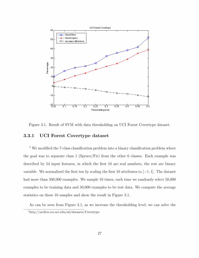
Figure 3.1. Result of SVM with data thresholding on UCI Forest Covertype dataset.
3.3.1 UCI Forest Covertype dataset
1 We modified the 7-class classification problem into a binary classification problem where
the goal was to separate class 1 (Spruce/Fir) from the other 6 classes. Each example was
described by 54 input features, in which the first 10 are real numbers, the rest are binary
variable. We normalized the first ten by scaling the first 10 attributes to [−1, 1]. The dataset
had more than 500,000 examples. We sample 10 times, each time we randomly select 50,000
examples to be training data and 50,000 examples to be test data. We compute the average
statistics on these 10 samples and show the result in Figure 3.1.
As can be seen from Figure 3.1, as we increase the thresholding level, we can solve the
1http://archive.ics.uci.edu/ml/datasets/Covertype
27
t = 0 t = 0.02 t = 0.04 t = 0.06 t = 0.08 t = 0.1’polygon’ ’polygon’ ’polygon’ ’polygon’ ’polygon’ ’pov’
’animation’ ’animation’ ’animation’ ’tiff’ ’pov’ ’graphics’’tiff’ ’sphere’ ’tiff’ ’graphics’ ’graphics’ ’polygon’
’graphics’ ’tiff’ ’graphics’ ’pov’ ’animation’ ’tiff’’cview’ ’graphics’ ’sphere’ ’sphere’ ’tiff’ ’sphere’’sphere’ ’images’ ’pov’ ’images’ ’sphere’ ’cview’
’pov’ ’cview’ ’images’ ’cview’ ’cview’ ’images’’images’ ’pov’ ’cview’ ’animation’ ’images’ ’bezier’’mpeg’ ’mpeg’ ’bezier’ ’bezier’ ’bezier’ ’animation’’image’ ’image’ ’mpeg’ ’diablo’ ’image’ ’wireframe’
Table 3.1. Top 10 keywords obtained with topic comp.graphics as the thresholding levelincreases. The top keywords do not change significantly when more thresholding applies.
problem faster (blue line) and use less memory (red line) to store the data by sacrificing
some minor amount of accuracy (black line).
3.3.2 20 Newsgroup Dataset
This dataset consist of Usenet articles Lang collected from 20 different newsgroups (e.g.
comp.graphics, comp.windows.x, misc.forsale, sci.space, talk.reglision.misc, etc.) which con-
tains an overall number of 20000 documents. Except for a small fraction of the articles, each
document belongs to exactly one newsgroup. The task is to learn which newsgroup an article
was posted to. The dataset is divided so that the training set contains 2/3 the number of
examples and the test set contains the rest. The dimension of the problem is 61K (number
of words in the dictionary). For each document, word we compute the corresponding TFIDF
score and then threshold the data based on TF-IDF score.
In Table 3.1, we show the list of top 20 keywords obtained with topic comp.graphics as
we varied the thresholding level, as can be seen as we increase the thresholding levels the top
28
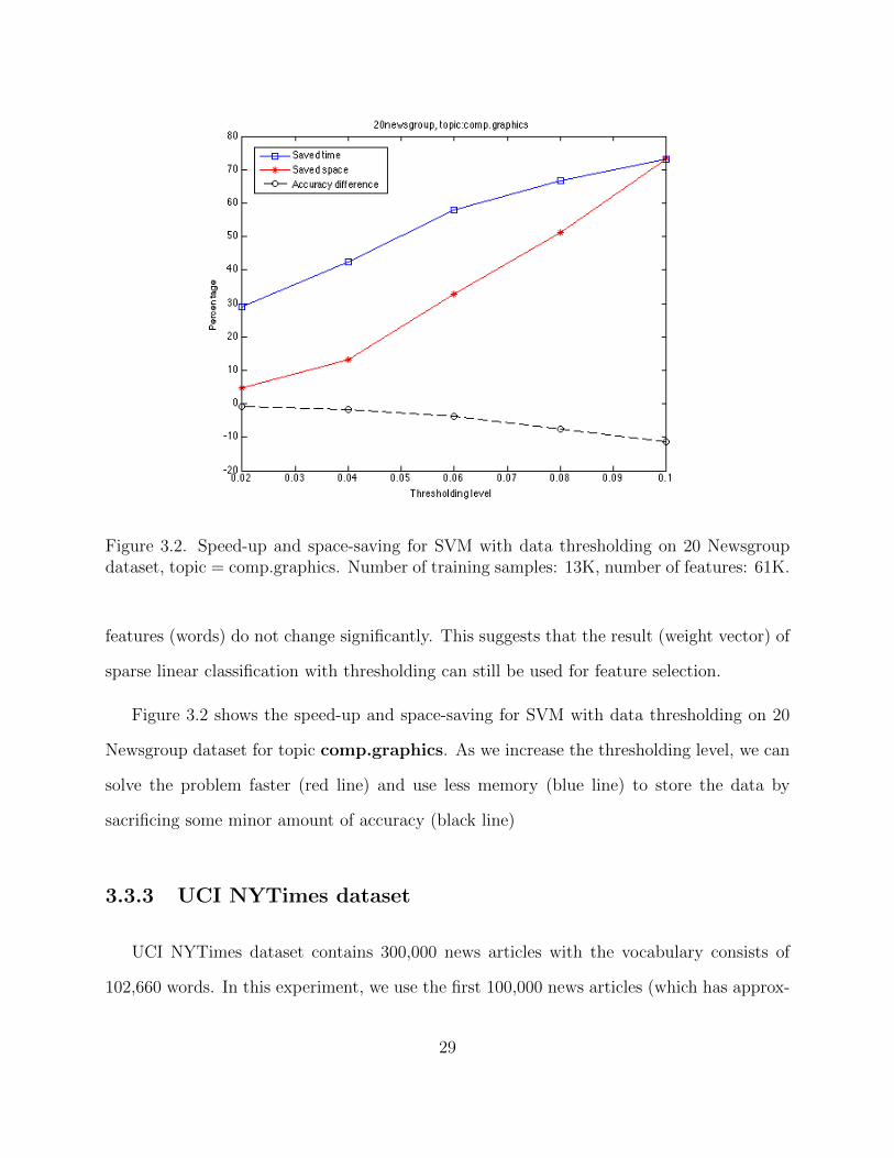
Figure 3.2. Speed-up and space-saving for SVM with data thresholding on 20 Newsgroupdataset, topic = comp.graphics. Number of training samples: 13K, number of features: 61K.
features (words) do not change significantly. This suggests that the result (weight vector) of
sparse linear classification with thresholding can still be used for feature selection.
Figure 3.2 shows the speed-up and space-saving for SVM with data thresholding on 20
Newsgroup dataset for topic comp.graphics. As we increase the thresholding level, we can
solve the problem faster (red line) and use less memory (blue line) to store the data by
sacrificing some minor amount of accuracy (black line)
3.3.3 UCI NYTimes dataset
UCI NYTimes dataset contains 300,000 news articles with the vocabulary consists of
102,660 words. In this experiment, we use the first 100,000 news articles (which has approx-
29
1 stock 11 bond2 nasdaq 12 forecast3 portfolio 13 thomson financial4 brokerage 14 index5 exchanges 15 royal bank6 shareholder 16 fund7 fund 17 marketing8 investor 18 companies9 alan greenspan 19 bank10 fed 20 merrill
Table 3.2. SVM Result: Top 20 keywords for topic ’stock’ on UCI NYTimes dataset withthresholding level of 0.05 on TF-IDF score (reduced dataset is only 3% of the full dataset).Total runtime: 4317s
imately 30 millions words in the collection) for training task. It is impossible to train SVM
with the whole dataset on a laptop/PC, so in this experiment we will just run SVM on the
thresholded dataset (by TF-IDF scores) and then report the top features in Table 3.2. The
thresholded dataset size with the thresholding level 0.05 only contains 850,000 non-zeroes,
which is roughly 3% of the full dataset.
30
Chapter 4
Low-rank Approximation
4.1 Introduction
A standard task in scientific computing is to determine for a given matrix A ∈ Rn×d an
approximate decomposition A ≈ BC where B ∈ Rn×k, C ∈ Rk×d; k is called the numerical
rank of the matrix. When k is much smaller than either n or d, such decomposition allows
the matrix to be stored inexpensively, and to be multiplied to vectors or other matrices
quickly.
Low-rank approximation has been used for solving many large-scale problems that in-
volves large amounts of data. By replacing the original matrices with approximated (low-
rank) ones, the perturbed problems often requires much less computational effort to solve.
Low-rank approximation methods have been shown to be successful on a variety of learning
tasks, such as Spectral partitioning for image and video segmentation Fowlkes et al. (2004),
Manifold learning Talwalkar et al. (2008). Recently, there have been interesting works on
using low-rank approximation in Kernel learning: Fine and Scheinberg (2002) proposed an
efficient method for kernel SVM learning problem by approximating the kernel matrix by a
31
low-rank positive semidefinite matrix. Bach and Jordan (2005) and Zhang et al. (2012) also
proposed similar approaches for more general kernel learning problems which also exploit
side information in the computation of low-rank decompositions for kernel matrices.
One important point worth noting here is that all of the above works just replace the
original data matrices directly with the low-rank ones, and then provide a bound on the error
made by solving the perturbed problem compared to the solution of the original problem. In
this thesis, we propose a new modeling approach that takes into account the approximation
error made when replacing the original matrices with low-rank approximations to modify
the original problem accordingly, via robust optimization perspective.
In this chapter, we focus on solving LASSO problem:
min‖β‖1≤λ
‖y −XTβ‖2 (4.1.1)
However, the result can also be generalized to more supervised learning problems:
minv∈R,w∈C
f(ATw + cv) (4.1.2)
where the loss function f : Rn → R is convex, the data matrix A ∈ Rd×n and vector c ∈ Rn
are given, C ⊆ Rd is a convex set that constraining the decision variable w.
In practice, a low-rank approximation may not be directly available, but has to be com-
puted. While the effort in finding low-rank approximation is typically linear in the size of
data matrix, in our approach leads to the biggest savings in what we refer to as the repeated
instances setup. In such a setup, the task is to solve multiple instances of similar programs,
where all the instances involve a common (or very similar) coefficient matrix. In that setup,
of which we provide real-world examples later, it makes sense to invest some effort in finding
the low-rank approximation once, and then exploit the same low-rank approximation for
each instance. The robust low-rank approach then offers enormous computational savings,
and produces solutions that are guaranteed to be feasible for the original problem.
32
4.2 Algorithms for Low-rank Approximation
In general, to find rank-k approximation of a matrix A ∈ Rn×d, we wish to find matrices
B ∈ Rn×k, C ∈ Rk×d such that the spectral norm/largest singular value norm error ‖A −
BC‖2 is minimal. The truncated singular value decomposition is known to provide the best
low-rank approximation for any given fixed rank Eckart and Young (1936); however, it is also
very costly to compute. There have been many different approaches proposed for computing
low-rank approximations, such as rank-revealing factorization (QR or LU) Gu and Eisenstat
(1996); Miranian and Gu (2003), subspace iteration methods, Lancoz algorithms Demmel
and Heath (1997). Recently, randomized algorithms have been developed and proved to be
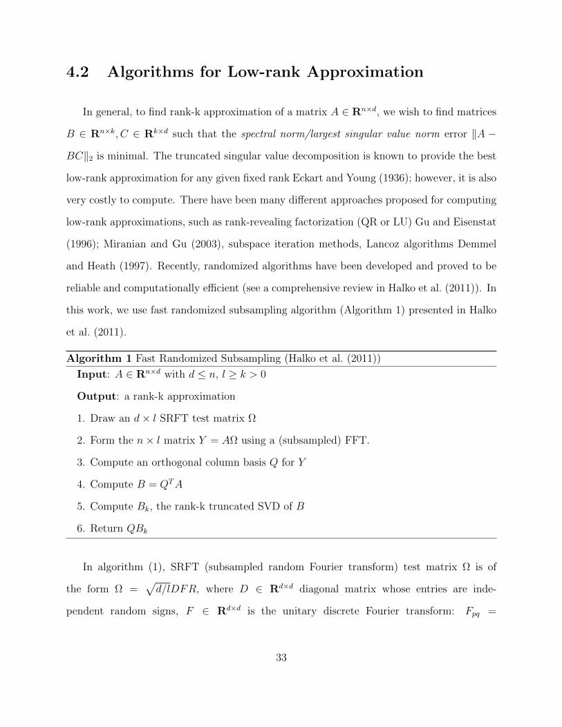
reliable and computationally efficient (see a comprehensive review in Halko et al. (2011)). In
this work, we use fast randomized subsampling algorithm (Algorithm 1) presented in Halko
et al. (2011).
Algorithm 1 Fast Randomized Subsampling (Halko et al. (2011))
Input: A ∈ Rn×d with d ≤ n, l ≥ k > 0
Output: a rank-k approximation
1. Draw an d× l SRFT test matrix Ω
2. Form the n× l matrix Y = AΩ using a (subsampled) FFT.
3. Compute an orthogonal column basis Q for Y
4. Compute B = QTA
5. Compute Bk, the rank-k truncated SVD of B
6. Return QBk
In algorithm (1), SRFT (subsampled random Fourier transform) test matrix Ω is of
the form Ω =√d/lDFR, where D ∈ Rd×d diagonal matrix whose entries are inde-
pendent random signs, F ∈ Rd×d is the unitary discrete Fourier transform: Fpq =
33
d−1/2 exp (−2πi(p− 1)(q − 1)/d) and R ∈ Rd×l which samples l coordinates from d uni-
formly at random.
Computing Y = AΩ can be done in O(nd log(l)) flops via a subsampled fast Fourier
transform. If A has special structure (e.g. sparsity) this can be fastened to O(lNA+(n+d)k2)
where NA is the number of non-zero entries in A.
When l ≥ Ω((k + log(kd)) log(k)) then with high probability we have:
‖A−QBk‖ ≤ O
(√d
l
)σk+1(A).
4.2.1 First order methods with Low-rank approximation
There has been extensive research on algorithms for solving the constrained LASSO
problem. Tibshirani (1996), Osborne et al. (2000) and Efron et al. (2004) amongst many
others developed algorithms using quadratic programming methods. These algorithms often
need to compute matrix inversions repeatedly, the computational cost increases rapidly as
the input size increases and hence they might not be applicable to very large scale datasets.
First order methods have also been used to solve the constrained LASSO problem:
NESTA - Nesterov’s proximal gradient method by Becker et al. (2011), GPSR - projected
gradient method by Figueiredo et al. (2007), PGN - projected quasi-Newton algorithm by
Schmidt et al. (2009), SPG - Spectral projected gradient algorithm by Birgin et al. (2003),
etc. In this work, we will use SPG (Algorithm 2) to solve LASSO and its variations, due
to its effectiveness for very large-scale convex optimization. SPG is also known to be more
efficient than classical gradient projected method due to spectral step length selection and
non-monotone search Birgin et al. (2003); Figueiredo et al. (2007); van den Berg et al. (2008).
However, our work can be applied to any first-order algorithm for solving the constrained
LASSO problem.
34

Algorithm 2 Spectral Projected Gradient Algorithm (Birgin et al. (2000))
goal: minx∈C
f(x), where f : Rn → R convex, differentiable; C ⊆ Rn is a closed convex set.
parameters: steplength bound parameters αmax > αmin > 0; safeguarding parameters
0 < σ1 < σ2 < 1; γ ∈ (0, 1).
initialize k = 0, x(0) ∈ C, α0 ∈ [αmin, αmax].
while ‖PC(x(k) −∇f(x(k)))− x(k)‖ ≥ ε do
1. compute d(k) = PC(x(k) − αk∇f(x(k))
)− x(k)
2. line search
(i) set x+ ← x(k) + d(k), η = 1 and δ ← ∇f(x(k))Td(k)
(ii) while f(x+) > max0≤j≤min(k,M)
f(x(k−j))+ γηδ
• compute η =−η2δ
2(f (x+)− f (x(k))− ηδ)
• if η ≥ σ1η and η ≤ σ2η then set η ← η, else set η ← η/2
• set x+ ← x(k) + ηd(k)
(iii) set steplength ρk ← η
3. set x(k+1) = x(k) + ρkd(k), s(k) = x(k+1) − x(k), and y(k) = ∇f(x(k+1))−∇f(x(k))
4. if (s(k))Ty(k) ≤ 0 then set αk+1 ← αmax
else set αk+1 ← min
(max
((s(k))T s(k)
(s(k))Ty(k), αmin
), αmax
)5. set k ← k + 1
(PC(z) denotes the projection of vector z onto the set C : PC(z) = arg minw∈C ‖z − w‖)
35
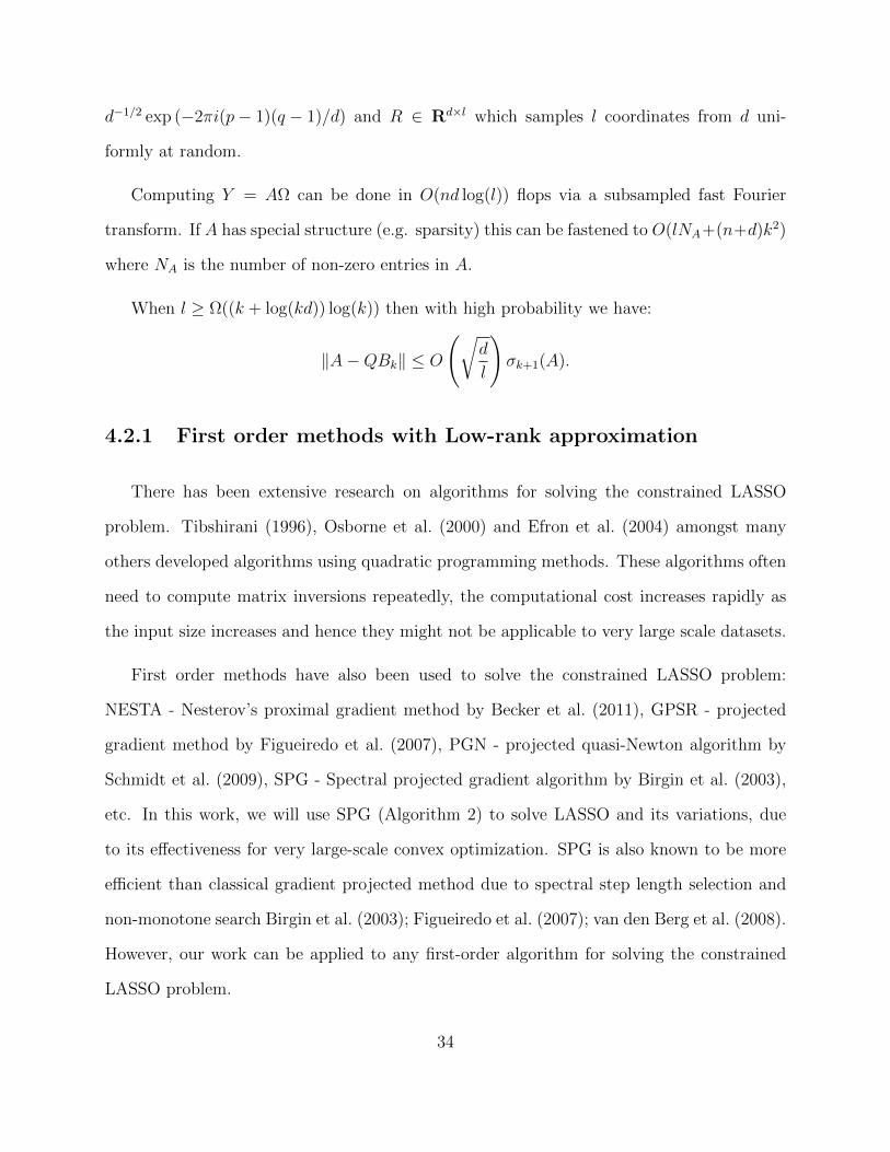
For sparse learning problems such as LASSO, the set C is the l1-ball B1(λ) = w :
‖w‖1 ≤ λ. We adopt the following algorithm developed by Duchi et al. (2008) to compute
projections onto the l1 ball efficiently in linear time:
Algorithm 3 Linear time projection onto l1 ball (Duchi et al. (2008))
input: z ∈ Rd and λ > 0
initialize U = 1, . . . , d, s = 0, η = 0
while U 6= ∅ do
1. pick k ∈ U randomly.
2. partition U into G = j ∈ U |zj ≥ zk, L = U \G
3. if (s+∑
j∈G zj)− (η + |G|)zk < λ then s← s+∑
j∈G zj; η ← η + |G|;U ← L
4. else U ← G \ k
set θ = (s− λ)/η
output w = max(zi − θ, 0)di=1
We now show how to use low-rank approximation to speedup first order methods. As
we will see, the speedup when applying our approach will be achieved with any first order
algorithm that involves computing the gradient. Generally, first-order method for LASSO
requires us to compute the gradient of the objective function in which for the constrained
LASSO problem, it is of the form:
∇β‖y −XTβ‖2 = XXTβ − y‖XTβ − y‖2
Finding such gradient involves computing the product of a matrix X ∈ Rn×d and a vector
u ∈ Rd as well as the product of XT with a vector v ∈ Rn. Each operation costs O(nd)
flops for dense matrix X or O(N) flops for sparse matrix X with N non-zero entries.
36
Assuming that the data matrix has a low-rank structure, that is X ≈ UV T where U ∈
Rn×k, V ∈ Rd×k with k << min(n, d). We can then exploit the low-rank structure in
order to improve the efficiency of the above matrix-vector multiplication by writing Xu =
U(V Tu). Computing z = V Tu costs O(kd) flops, and computing Uz costs O(kn) flops,
thus the total number of flops is O(k(n + d)). This is a significant improvement compared
to the cost of matrix-vector multiplication on the original data matrix, especially when
X is dense, high dimensional and approximately low-rank. When X is sparse and k is
much smaller than the average number of non-zero entries per sample, the matrix-vector
multiplication computation that exploits the low-rank structure is also much faster than
direct multiplication. Furthermore, the space complexity required to store the low-rank
approximation is only O(k(n + d)) compared to O(nd) when X is dense or O(N) if X is a
sparse matrix.
For more general supervised learning problem (4.1.2), we could also compute the gradient
exploiting the low-rank structure of the data matrix: suppose that A = V UT where U ∈
Rn×k, V ∈ Rd×k with k << min(n, d), let h(w, v) = f(ATw + cv), the gradient can be
computed as following:
∇wh(w, v) = A∇f(ATw + cv) = V UT∇f(UV Tw + cv)
∇vh(w, v) = cT∇f(ATw + bv) = cT∇f(UV Tw + cv)
Similarly, the cost of computing the above gradient is only O(k(n + d)) for dense data
matrix X or O(N) for sparse one.
4.3 Robust Low-rank LASSO
Important questions worth asking when replacing the original data matrix by a low-rank
approximation are “how much information do we lose?”, and “how does it effect the LASSO
37

problem?”. In this section, we will examine the effect of using low-rank approximation, or
in other words, thresholding the singular values of the data matrix according to an absolute
threshold level εk. We replace the matrix X by X, the closest (in largest singular value
norm) rank-k approximation to X, and the error ∆ := X −X satisfies ‖∆‖ ≤ εk, where ‖ · ‖
denotes the largest singular value norm.
As seen in previous section, computing the low-rank approximation of a matrix is feasible
even in a large scale setting. Our basic goal is to end up solving a slightly modified LASSO
problem using rank-k approximation, while controlling for the error made.
We want to take into account the worst-case error in the objective function that is made
upon replacing X with its rank-k approximation, X. To this end, we consider the following
robust counterpart to (4.1.1):
ψεk,λ(X) := min‖β‖1≤λ
max‖X−X‖≤εk
∥∥y −XTβ∥∥
2
= min‖β‖1≤λ
max‖∆‖≤εk
∥∥∥y − (X −∆)Tβ∥∥∥
2
(4.3.1)
Let us define f(z) = ‖z‖2, we have:
38

max‖∆‖≤εk
∥∥∥y − (X −∆)Tβ∥∥∥
2= max‖∆‖≤εk
f(y − XTβ + ∆Tβ)
= max‖∆‖≤εk
maxu∈Rm
uT (y − XTβ + ∆Tβ)− f ∗(u)
= max
u∈Rm
uT (y − XTβ)− f ∗(u) + max
‖∆‖≤εkuT∆Tβ
= max
u∈Rm
uT (y − XTβ)− f ∗(u) + max
‖∆‖≤εk〈∆T , βuT 〉
= max
u∈Rm
uT (y − XTβ)− f ∗(u) + εk‖βuT‖∗
= max
u∈Rm
uT (y − XTβ)− f ∗(u) + εk‖β‖2‖u‖2
= max
u∈Rm
uT (y − XTβ)− f ∗(u) + max
‖z‖2≤εk‖β‖2uT z
= max‖z‖2≤εk‖β‖2
maxu∈Rm
uT (y − XTβ + z)− f ∗(u)
= max‖z‖2≤εk‖β‖2
f(y − XTβ + z)
= max‖z‖2≤εk‖β‖2
‖y − XTβ + z‖2
= ‖y − XTβ‖2 + εk‖β‖2
here ‖.‖∗ is the nuclear norm (the dual of spectral norm) and f ∗ is the conjugate dual of f .
Therefore, we can write the robust counterpart of LASSO problem in (2) as:
ψεk,λ(X) = min‖β‖1≤λ
‖y − XTβ‖2 + εk‖β‖2 (4.3.2)
Let g(β) = ‖y − XTβ‖2 + εk‖β‖2, its gradient is:
∇βg(β) = XXTβ − y‖XTβ − y‖2
+ εkβ
‖β‖2
Hence the cost of computing this gradient is also similar as for the low-rank LASSO problem,
which is O(k(n+ d)).
39

4.3.1 Theoretical Analysis
In this section, we present some theoretical analysis for the Low-rank LASSO models, in
particular we bound how far their solutions from the true weight vector. In order to do so,
we will need the following definitions:
Restricted nullspace (Cohen et al. (2009)): for a given subset S ⊆ 1, . . . , d and a
constant α ≥ 1, define:
C(S, α) := θ ∈ Rd : ‖θSC‖1 ≤ α‖θS‖1
Given k ≤ d, the matrix X is said to satisfy the restricted nullspace condition of order k if
null(X) ∩ C(S, 1) = 0,∀S ⊆ 1, . . . , d : |S| = k.
Restricted eigenvalue (Bickel et al. (2008)): the sample covariance matrix XTX/n is
said to satisfy the restricted eigenvalue condition over a set S with parameters α ≥ 1, γ > 0
if 1n‖Xθ‖2
2 ≥ γ2‖θ‖22,∀θ ∈ C(S, α). We denote that X ∈ RE(S, α, γ) if the above condition
is true.
Main result: we consider the classical linear model with noisy settings: y = Xβ∗ + w,
where y ∈ Rn is the vector of responses, the matrix X ∈ Rn×d is feature matrix, and w ∈ Rd
is a random white noise vector: w ∼ N (0, σ2In×n). Let define:
β(λ) = arg min‖β‖1≤λ
‖y −Xβ‖2
β(λ, η) = arg min‖β‖1≤λ
‖y − Xβ‖2 + η‖β‖2
Hence, β(λ, εk) is the solution for the robust counterpart optimization problem (4.3.2) and
β(λ, 0) is the solution for the LASSO problem if we just replace the feature matrix X by its
low rank approximation X.
We will now show that when the feature matrix X is “close“ to low-rank (i.e. εk is small),
the estimators β(λ, η) is closed to the optimal weight vector β∗ for any 0 ≤ η ≤ εk.
40

To shorten the equations, we abbreviate β(λ, η) as β.
We also use standard assumptions as for nominal LASSO problem as in Raskutti et al.
(2010):
(a) λ = ‖β∗‖1, S is the support of β∗ and |S| = p.
(b) X ∈ RE(S, 1, γ) for some γ > 0.
Since ‖∆x‖2 ≤ ‖∆‖2‖x‖2 ≤ εk‖x‖2, we have:
‖y −Xβ‖2 = ‖y − Xβ + ∆β‖2
≤ ‖y − Xβ‖2 + ‖∆β‖2
≤ ‖y − Xβ‖2 + εk‖β‖2
=(‖y − Xβ‖2 + η‖β‖2
)+ (εk − η)‖β‖2
≤(‖y − Xβ‖2 + η‖β‖2
)+ (εk − η)‖β‖2
=(‖y −Xβ −∆β‖2 + η‖β‖2
)+ (εk − η)‖β‖2
≤(‖y −Xβ‖2 + ‖∆β‖2 + η‖β‖2
)+ (εk − η)‖β‖2
≤ ‖y −Xβ‖2 + (εk + η)‖β‖2 + (εk − η)‖β‖2
≤ ‖y −Xβ∗‖2 + (εk + η)‖β‖2 + (εk − η)‖β‖2
In addition, ‖β‖2 ≤ ‖β‖1 ≤ λ, ‖β‖2 ≤ ‖β‖1 ≤ λ, so:
‖y −Xβ‖2 ≤ ‖y −Xβ∗‖2 + 2εkλ (4.3.3)
Now let ζ = β∗− β, we can write y = Xβ∗+w as y−Xβ = Xζ+w, therefore (4.3.3) implies
that:
‖Xζ + w‖2 ≤ ‖w‖2 + 2εkλ
⇒ ‖Xζ + w‖22 ≤ (‖w‖2 + 2εkλ)2
⇒ ‖Xζ‖22 ≤ 4εkλ‖w‖2 + 4ε2kλ
2 − 2ζTXTw
⇒ 1
n‖Xζ‖2
2 ≤4εkλ
n‖w‖2 +
4ε2kλ2
n+ 2‖ζ‖1
∥∥∥∥XTw
n
∥∥∥∥∞
41
Using assumption (a), we obtain:
‖βSC‖1 + ‖βS‖1 = ‖β‖1 ≤ λ = ‖β∗‖1 = ‖β∗S‖1
⇒ ‖βSC‖1 ≤ ‖β∗S‖1 − ‖βS‖1 ≤ ‖β∗S − βS‖1
⇒ ‖β∗SC − βSC‖1 ≤ ‖β∗S − βS‖1
⇒ ‖ζSC‖1 ≤ ‖ζS‖1 ⇒ ζ ∈ C(S, 1) and
‖ζ‖1 ≤ 2‖ζS‖1 ≤ 2√p‖ζS‖2 ≤ 2
√p‖ζ‖2
Using assumption (b) X ∈ RE(S, 1, γ) and the fact that ζ ∈ C(S, 1), we have 1n‖Xζ‖2
2 ≥
γ2‖ζ‖22, therefore:
γ2‖ζ‖22 ≤
4εkλ
n‖w‖2 +
4ε2kλ2
n+ 4√p‖ζ‖2
∥∥∥∥XTw
n
∥∥∥∥∞
(4.3.4)
Lemma 4 (Wainwright (2010)) Suppose X is bounded by L, i.e. |Xij| ≤ L, w ∼
N (0, σ2In×n) then with high probability we have:∥∥∥∥XTw
n
∥∥∥∥∞≤ L
√3σ2 log d
n
Lemma 5 Suppose w ∼ N (0, σ2In×n) and c > 1, then with probability at least 1−e− 316n(c−1)2
we have:
‖w‖2 ≤√σcn
Proof: Since w ∼ N (0, σ2In×n), Z =∑n
i=1(wi/σ)2 ∼ χ2n, using the tail bound for
Chi-square random variable by Johnstone (2000), for any ρ > 0 we have:
P [|Z − n| ≥ nρ] ≤ exp
(− 3
16nρ2
),
Thus, by setting ρ = c − 1, with probability at least 1 − e− 316n(c−1)2 we have Z ≤ cn, i.e.
‖w‖2 ≤√σcn.
42
Assuming L, σ, λ are constants, using (4.3.4) and the results of Lemma 1 and 2, with
high probability we have:
‖ζ‖22 ≤ O
(εk√n
)+O
(ε2kn
)+O
(√p log d
n
)‖ζ‖2
Solving this inequality we obtain the upper bound on ‖β∗−β‖2 = ‖ζ‖2 (with high probability)
as following:
‖β∗ − β(λ, η)‖2 ≤ O
(√p log d
n+
εk√n
+ε2kn
)The above result shows that when the error made by replacing the feature matrix with its
low-rank approximation (LR-LASSO) is small enough compared to√n (i.e. εk <<
√n), the
corresponding estimator β(λ, 0) (for LR-LASSO) is closed to the optimal solution β∗. The
solution of the robust counterpart of LASSO (RLR-LASSO) which is β(λ, εk), is also closed
to the optimal solution β∗.
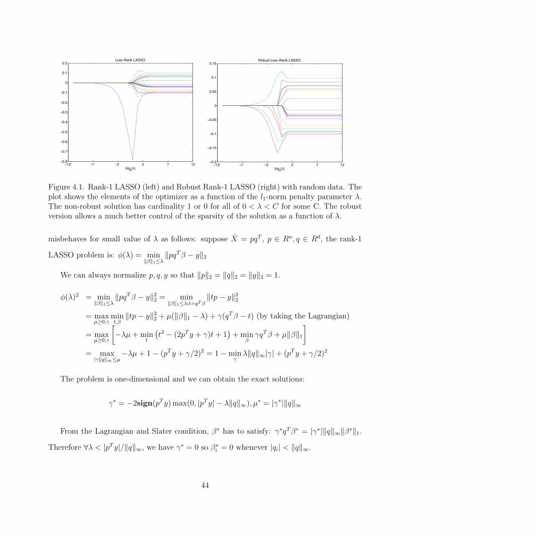
4.3.2 Discussion
One might ask what happen if we just use the low-rank approximation matrix directly.
We will show that we might end up with unexpected solutions if we do so. Indeed, we consider
the rank 1 LASSO problem in which the data matrix X is approximated with rank-1 matrix
X = uvT for some u ∈ Rn, v ∈ Rd: min‖β‖1≤λ ‖y − uvTβ‖2. We randomly generate two
vector u ∈ R20, v ∈ R20 and solve the rank-1 LASSO problem for λ = 2−12, . . . , 212, figure
4.1 shows the sparsity pattern of the solution of rank-1 LASSO vs robust rank-1 LASSO
problem.
We can also explain analytically the reason why solution of non-robust rank-1 LASSO
43
−12 −7 −2 2 7 12−0.8
−0.7
−0.6
−0.5
−0.4
−0.3
−0.2
−0.1
0
0.1
0.2
log2(λ)
Low−Rank LASSO
−12 −7 −2 2 7 12−0.2
−0.15
−0.1
−0.05
0
0.05
0.1
0.15
log2(λ)
Robust Low−Rank LASSO
Figure 4.1. Rank-1 LASSO (left) and Robust Rank-1 LASSO (right) with random data. Theplot shows the elements of the optimizer as a function of the l1-norm penalty parameter λ.The non-robust solution has cardinality 1 or 0 for all of 0 < λ < C for some C. The robustversion allows a much better control of the sparsity of the solution as a function of λ.
misbehaves for small value of λ as follows: suppose X = pqT , p ∈ Rn, q ∈ Rd, the rank-1
LASSO problem is: φ(λ) = min‖β‖1≤λ
‖pqTβ − y‖2
We can always normalize p, q, y so that ‖p‖2 = ‖q‖2 = ‖y‖2 = 1.
φ(λ)2 = min‖β‖1≤λ
‖pqTβ − y‖22 = min
‖β‖1≤λ;t=qT β‖tp− y‖2
2
= maxµ≥0,γ
mint,β‖tp− y‖2
2 + µ(‖β‖1 − λ) + γ(qTβ − t) (by taking the Lagrangian)
= maxµ≥0,γ
[−λµ+ min
t
(t2 − (2pTy + γ)t+ 1
)+ min
βγqTβ + µ‖β‖1
]= max|γ‖q‖∞≤µ
−λµ+ 1− (pTy + γ/2)2 = 1−minγλ‖q‖∞|γ|+ (pTy + γ/2)2
The problem is one-dimensional and we can obtain the exact solutions:
γ∗ = −2sign(pTy) max(0, |pTy| − λ‖q‖∞), µ∗ = |γ∗|‖q‖∞
From the Lagrangian and Slater condition, β∗ has to satisfy: γ∗qTβ∗ = |γ∗|‖q‖∞‖β∗‖1.
Therefore ∀λ < |pTy|/‖q‖∞, we have γ∗ = 0 so β∗i = 0 whenever |qi| < ‖q‖∞.
44

4.3.3 Regularized Robust Rank-1 LASSO
In this section, we consider a special case in which the rank of the approximated matrix
X is exactly 1. Note that the constrained LASSO and regularized LASSO are related -
via Lagrangian. Similar to constrained LASSO problem, we can also formulate the robust
regularized LASSO as following:
minw‖y − XTβ‖2 + ε‖β‖2 + λ‖β‖1
When X is exactly rank-one, regularized robust LASSO problem becomes very easy -
one-dimensional. Suppose that XT = pqT for some p ∈ Rn, q ∈ Rd, the robust counterpart
is expresses as:
ψε,λ(p, q) = minβ‖qpTβ − y‖2 + ε‖β‖2 + λ‖β‖1. (4.3.5)
We can always normalize p, q so that ‖p‖2 = ‖q‖2 = 1. Indeed, upon replacing λ (resp.
ε) by ‖p‖2‖q‖2λ (resp. ‖p‖2‖q‖2ε), we are back to the normalized case ‖p‖2 = ‖q‖2 = 1.
Finally, we can divide both values λ, ε by ‖y‖2 to reduce further our problem to one with
‖y‖2 = 1. We have:
ψε,λ(p, q) = minβ, t=βT p
‖tq − y‖2 + ε‖β‖2 + λ‖β‖1
Using Lagrangian with multiplier µ, we obtain
ψε,λ(p, q) = maxµ
(mint‖tq − y‖2 + µt
)+
(minβ
ε‖w‖2 + λ‖β‖1 − µpTβ)
Let us define A(µ) := mint ‖tq − y‖2 + µt and B(µ) := minβ ε‖w‖2 + λ‖β‖1 − µpTβ.
The first term, A(µ), is −∞ when |µ| > 1. Otherwise, it can be expressed in terms of
45

c := qTy ∈ [−1, 1] and s =√
1− c2 ≥ 0 as follows:
A(µ) = mint‖tq − y‖2 + µt = min
t
√t2 − 2tc+ 1 + µt
= mint
√(t− c)2 + s2 + µt = µc+ min
ξ
√ξ2 + s2 − µξ [ξ = t− c]
= µc+ s√
1− µ2 [t∗ = c+ (µs)/√
1− µ2.]
The second term, B(µ), writes
B(µ) = minβ
ε‖β‖2 + λ‖β‖1 − µpTβ
= maxv,r
0 : µp = v + r, ‖v‖∞ ≤ λ, ‖r‖2 ≤ ε.
The quantity B(µ) is finite (and indeed, zero) if and only if there exist v such that
‖v‖∞ ≤ λ, ‖v − µp‖2 ≤ ε.
Hence, our problem becomes:
maxµ,v
µc+ s√
1− µ2 : |µ| ≤ 1, ‖v‖∞ ≤ λ, ‖v − µp‖2 ≤ ε.
Note that the function F (µ) := minv ‖v − µp‖2 : ‖v‖∞ ≤ λ has an optimal point
is v∗ = min(λ,max(−λ, µp)) in which the corresponding value is F (µ) = ‖(|µp| − λ1)+‖2.
Therefore, our problem is reduced to a one-dimensional problem:
maxµ
µc+ s√
1− µ2 : |µ| ≤ 1, ‖(|µp| − λ1)+‖2 ≤ ε.
The optimal µ is of the same sign as c, and the problem is equivalent to
maxµ
µ|c|+ s√
1− µ2 : 0 ≤ µ ≤ 1, ‖(µ|p| − λ1)+‖2 ≤ ε,
which can be easily solved by bisection in O(n). Note that the dependence on q is only via
c = qTy, s =√
1− c2. The cost of computing c is O(m), so the robust counterpart (4.3.5)
can be solved in O(n+m).
46
When ε = 0, we recover an ordinary LASSO problem with rank-one matrix:
maxµ
µ|c|+ s√
1− µ2 : 0 ≤ µ ≤ 1, µ‖p‖∞ ≤ λ.
4.4 Experimental Results
The purpose of our experiments is to compare the performance of LASSO, LR-LASSO
and RLR-LASSO in two different tasks: multi-label classification (4.1) and word associations
for multiple queries (4.2).
For models using low-rank approximation (LR-LASSO and RLR-LASSO), we first run
experiments computing low-rank approximation matrices with different values of k using Fast
randomized subsampling algorithm. The low-rank dimension k is ranging from 5 to 50, and
l is set to k+10. Figure 1 shows the running time of computing the low-rank approximation
for different datasets as k varied; the ratio σk+1/σ1 is also reported. As can be seen from the
table, low-rank approximation can be computed quickly even for large datasets with million
of samples and hundreds of thousands of features. The (k + 1)th singular value is also small
compared to the largest singular value of the data matrix.
For the experiments presented in this section, we chose ε = 10−6, γ = 10−4, σ1 = 0.1, σ2 =
0.9,M = 10, αmin = 10−3, αmax = 103, σ0 = 1 as suggested by Birgin et al. (2001). The
regularization parameter λ is tuned from 10i : i = 3, 4, 5, 6 using five-fold cross-validation
on the training data (with F1-score for each one-vs-all sub-classification instance).
All experiments are conducted on a personal workstation with 16GB RAM and 2.6GHz
quad-core Intel processor.
47
4.4.1 Datasets
RCV1-V2: Reuters Corpus Volume 1 - Version 2 is a large-scale dataset for text classi-
fication task that is based on the well known benchmark dataset for text classification, the
Reuters (RCV1) dataset. In our experiments, we use the full topics set containing 804,414
news articles, each article is assigned to a subset of 101 topics. We use the pre-processed
data that prepared by Lewis et al. (2004), which splits the data into 23,149 training docu-
ments and 781,265 test documents. The number of features in this dataset is 46, 236 and
the density of the data is 0.031.
TMC2007: Text Mining Competition dataset is based on the competition organized
by the text mining workshop of the 7Th SIAM international conference on data mining. It
contains 28,596 aviation safety reports in free text form, each annotated with a subset of
the 22 problem types that appear during certain flights. TMC2007 has 49,060 features and
density of 0.098.
PUBMED, NYTimes Datasets: we use two largest UCI Bag-of-word datasets 1: NY-
Times news articles dataset which contains 300,000 documents, 102,660 words and approxi-
mately 100,000,000 non-zero terms resulting in a file of size 1GB; and PUBMED abstracts
dataset which contains 8,200,000 documents, 141,043 words and approximately 730,000,000
non-zero terms giving a file size of 7.8GB.
Figure 4.2 shows the top 5000 singular values for each data, scaled by the maximum
singular value - as can be seen from the plot, the singular values decay quickly thus, we are
safe to say that the corresponding data matrices for the above datasets are approximately
low-rank. We believe that such phenomenon is also true for most text datasets.
1http://archive.ics.uci.edu/ml/datasets/Bag+of+Words
48
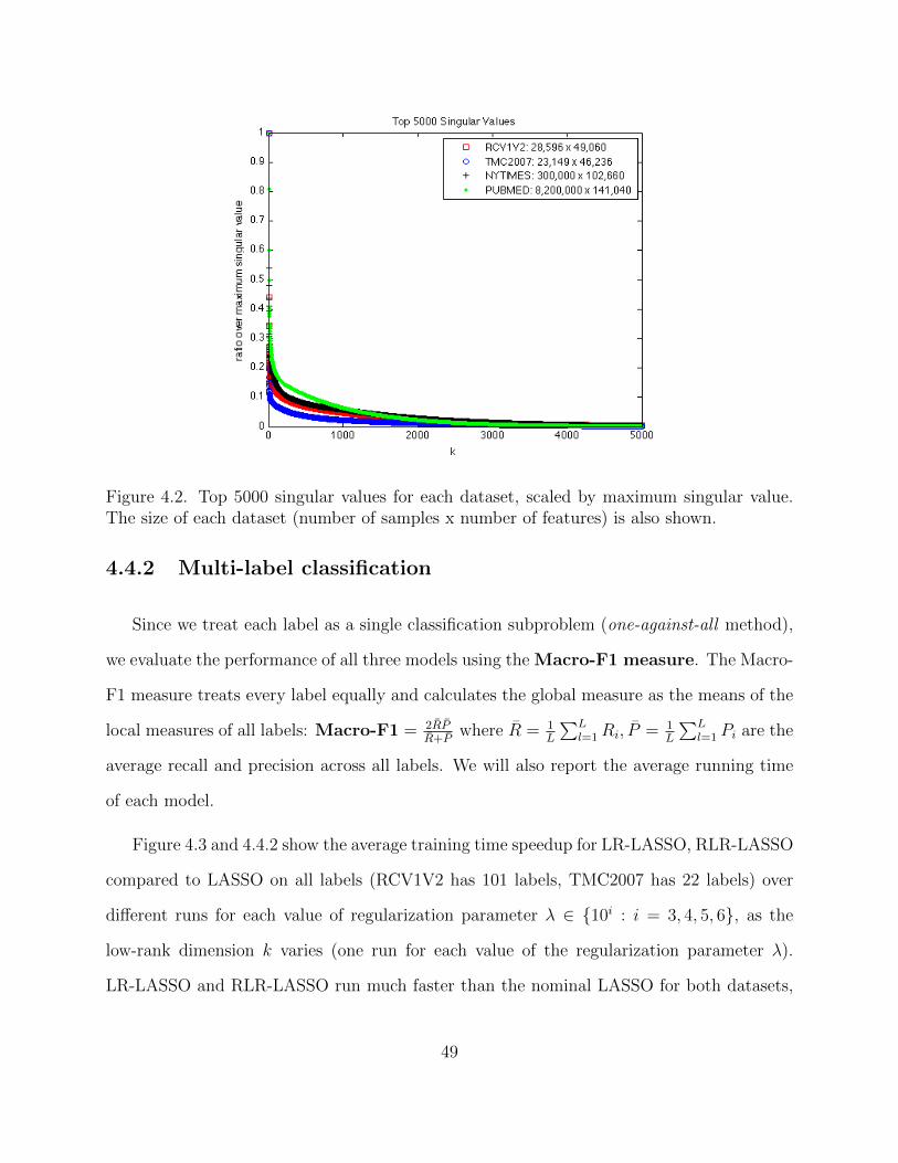
Figure 4.2. Top 5000 singular values for each dataset, scaled by maximum singular value.The size of each dataset (number of samples x number of features) is also shown.
4.4.2 Multi-label classification
Since we treat each label as a single classification subproblem (one-against-all method),
we evaluate the performance of all three models using the Macro-F1 measure. The Macro-
F1 measure treats every label equally and calculates the global measure as the means of the
local measures of all labels: Macro-F1 = 2RPR+P
where R = 1L
∑Ll=1Ri, P = 1
L
∑Ll=1 Pi are the
average recall and precision across all labels. We will also report the average running time
of each model.
Figure 4.3 and 4.4.2 show the average training time speedup for LR-LASSO, RLR-LASSO
compared to LASSO on all labels (RCV1V2 has 101 labels, TMC2007 has 22 labels) over
different runs for each value of regularization parameter λ ∈ 10i : i = 3, 4, 5, 6, as the
low-rank dimension k varies (one run for each value of the regularization parameter λ).
LR-LASSO and RLR-LASSO run much faster than the nominal LASSO for both datasets,
49
5 10 15 20 25 30 35 40 45 50−7
−6
−5
−4
−3
−2
−1
0
Low−rank dimension k
Macro F1−Score improvement over LASSO: RCV1V2
Perc
enta
ge (%
)
LR−LASSORLR−LASSO
5 10 15 20 25 30 35 40 45 50100
200
300
400
500
600
700
Low−rank dimension k
Training Time Speedup over LASSO: RCV1V2
Perc
enta
ge (%
)
LR−LASSORLR−LASSO
Figure 4.3. Multi-label classification: RCV1V2 dataset
around 3-6 times in magnitude. We also observe that RLR-LASSO run slightly faster than
LR-LASSO. Perhaps the l2 regularization term in the objective function of RLR-LASSO
model helps SPG algorithm converges faster than LR-LASSO.
As can also be seen from Figure 4.3 and 4.4.2, as k increases, the performances of low-rank
approximation models improve gradually. Although LR-LASSO does not perform anywhere
close to LASSO, its robust model RLR-LASSO has almost the same Macro F1-Score as the
nominal LASSO with a large enough k.
4.4.3 When labels are columns of data matrix
For many applications - especially in text classification such as in Gawalt et al. (2010),
the goal is to learn a short list of words that are predictive for a given query term in a text
dataset. LASSO can be used to produce such list of predictive words. To be manageable
by a human reader, the list should be very short w.r.t the number of features, thus we solve
the LASSO problem with different values of λ and choose the one that generates enough
non-zeros in the solution.
50
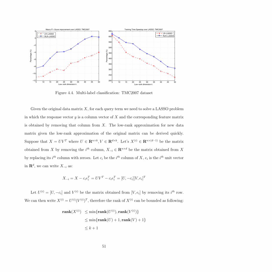
5 10 15 20 25 30 35 40 45 50−12
−10
−8
−6
−4
−2
0
2
Low−rank dimension k
Macro F1−Score improvement over LASSO: TMC2007
Perc
enta
ge (%
)
LR−LASSORLR−LASSO
5 10 15 20 25 30 35 40 45 50200
250
300
350
400
450
500
550
600
650
Low−rank dimension k
Training Time Speedup over LASSO: TMC2007
Perc
enta
ge (%
)
LR−LASSORLR−LASSO
Figure 4.4. Multi-label classification: TMC2007 dataset
Given the original data matrix X, for each query term we need to solve a LASSO problem
in which the response vector y is a column vector of X and the corresponding feature matrix
is obtained by removing that column from X. The low-rank approximation for new data
matrix given the low-rank approximation of the original matrix can be derived quickly.
Suppose that X = UV T where U ∈ Rn×k, V ∈ Rd×k. Let’s X(i) ∈ Rn×(d−1) be the matrix
obtained from X by removing the ith column, X−i ∈ Rn×d be the matrix obtained from X
by replacing its ith column with zeroes. Let ci be the ith column of X, ei is the ith unit vector
in Rd, we can write X−i as:
X−i = X − cieTi = UV T − cieTi = [U,−ci][V, ei]T
Let U (i) = [U,−ci] and V (i) be the matrix obtained from [V, ei] by removing its ith row.
We can then write X(i) = U (i)(V (i))T , therefore the rank of X(i) can be bounded as following:
rank(X(i)) ≤ minrank(U (i)), rank(V (i))
≤ minrank(U) + 1, rank(V ) + 1
≤ k + 1
51
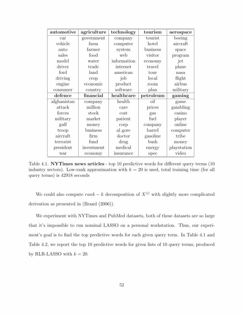
automotive agriculture technology tourism aerospacecar government company tourist boeing
vehicle farm computer hotel aircraftauto farmer system business spacesales food web visitor program
model water information economy jetdriver trade internet travel planeford land american tour nasa
driving crop job local flightengine economic product room airbus
consumer country software plan militarydefence financial healthcare petroleum gaming
afghanistan company health oil gameattack million care prices gamblingforces stock cost gas casino
military market patient fuel playergulf money corp company online
troop business al gore barrel computeraircraft firm doctor gasoline tribeterrorist fund drug bush moneypresident investment medical energy playstation
war economy insurance opec video
Table 4.1. NYTimes news articles - top 10 predictive words for different query terms (10industry sectors). Low-rank approximation with k = 20 is used, total training time (for allquery terms) is 42918 seconds
We could also compute rank − k decomposition of X(i) with slightly more complicated
derivation as presented in (Brand (2006)).
We experiment with NYTimes and PubMed datasets, both of these datasets are so large
that it’s impossible to run nominal LASSO on a personal workstation. Thus, our experi-
ment’s goal is to find the top predictive words for each given query term. In Table 4.1 and
Table 4.2, we report the top 10 predictive words for given lists of 10 query terms, produced
by RLR-LASSO with k = 20.
52
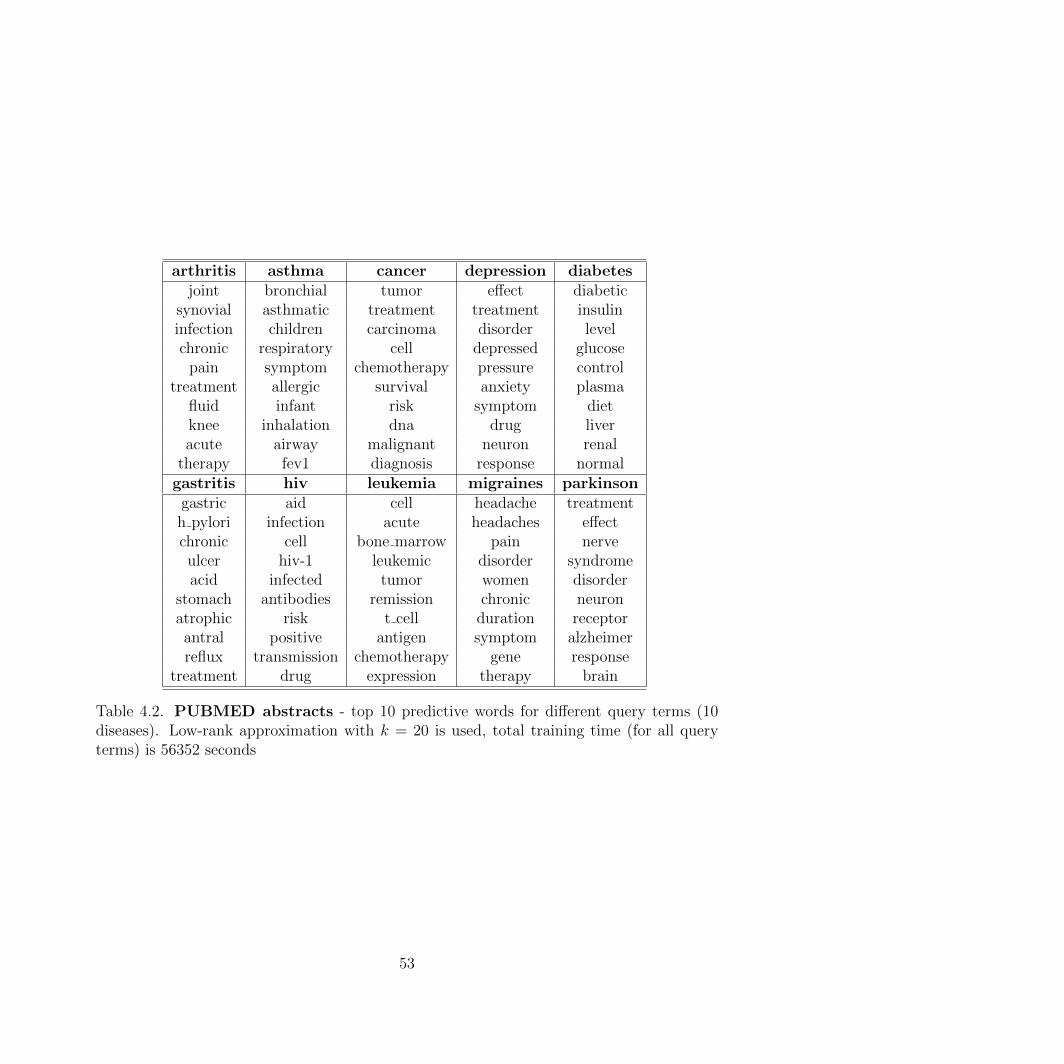
arthritis asthma cancer depression diabetesjoint bronchial tumor effect diabetic
synovial asthmatic treatment treatment insulininfection children carcinoma disorder levelchronic respiratory cell depressed glucose
pain symptom chemotherapy pressure controltreatment allergic survival anxiety plasma
fluid infant risk symptom dietknee inhalation dna drug liveracute airway malignant neuron renal
therapy fev1 diagnosis response normalgastritis hiv leukemia migraines parkinson
gastric aid cell headache treatmenth pylori infection acute headaches effectchronic cell bone marrow pain nerveulcer hiv-1 leukemic disorder syndromeacid infected tumor women disorder
stomach antibodies remission chronic neuronatrophic risk t cell duration receptorantral positive antigen symptom alzheimerreflux transmission chemotherapy gene response
treatment drug expression therapy brain
Table 4.2. PUBMED abstracts - top 10 predictive words for different query terms (10diseases). Low-rank approximation with k = 20 is used, total training time (for all queryterms) is 56352 seconds
53

Chapter 5
Conclusion
In this dissertation, we introduced new learning models that are capable of solving large
scale machine learning problems using data approximation under robust optimization per-
spective. We have showed that data approximation under robust scheme is efficient and
scalable and more reliable than just applying the approximation directly.
In Chapter 3, we have described data thresholding technique for large-scale sparse linear
classification and provided theoretical bound on the amount of thresholding level needed to
obtain desired performance. The proposed method is a promising pro-processing method
that can be applied in any learning algorithm to efficiently solve large-scale sparse linear
classification problems, both in terms of required memory as well as the running time of the
algorithm.
Next, in Chapter 4, we have described an efficient and scalable robust low-rank model
for LASSO problem, in which the approximation error made by replacing the original data
matrix with a low-rank approximation is taken into account in the model itself. The exper-
imental results lead us to believe that the proposed model could make statistical learning
that involves running multiple instances of LASSO feasible for extremely large datasets. Al-
54

though we only focus on first-order methods in which the main computational effort is to
compute the gradient, we believe that similar approach can be taken on how low-rank struc-
tures could help in speeding up second-order methods for solving LASSO problem. Another
interesting direction we also wish to pursue is to construct robust low-rank models for other
learning problems.
55

Bibliography
Anthony, M. and Bartlett, P. L. (1999). Neural Network Learning: Theoretical Foundations.
Cambridge University Press.
Bach, F. R. and Jordan, M. I. (2005). Predictive low-rank decomposition for kernel methods.
In Proceedings of the 22nd international conference on Machine learning, ICML ’05, pages
33–40, New York, NY, USA. ACM.
Balakrishnan, S. and Madigan, D. (2008). Algorithms for sparse linear classifiers in the
massive data setting. J. Mach. Learn. Res., 9:313–337.
Becker, S., Bobin, J., and Candes, E. J. (2011). Nesta: A fast and accurate first-order
method for sparse recovery. SIAM J. Imaging Sciences, 4(1):1–39.
Ben-Tal, A., El Ghaoui, L., and Nemirovski, A. (2009). Robust Optimization (Princeton
Series in Applied Mathematics). Princeton University Press.
Bhattacharyya, C. (2004). Robust classification of noisy data using second order cone pro-
gramming approach. In Intelligent Sensing and Information Processing, 2004. Proceedings
of International Conference on, pages 433 – 438.
Bhattachryya, S., Grate, L., Mian, S., Ghaoui, L. E., and Jordan, M. (2003). Robust
sparse hyperplane classifiers: application to uncertain molecular profiling data. Journal
of Computational Biology, 11(6):1073–1089.
56
Bickel, P. J., Ritov, Y., and Tsybakov, A. B. (2008). Simultaneous analysis of lasso and
dantzig selector.
Birgin, E. G., Martınez, J. M., and Raydan, M. (2000). Nonmonotone spectral projected
gradient methods on convex sets. SIAM Journal on Optimization, pages 1196–1211.
Birgin, E. G., Martınez, J. M., and Raydan, M. (2001). ACM Trans. Math. Softw., 27(3):340–
349.
Birgin, E. G., Martinez, J. M., and Raydan, M. (2003). Inexact spectral projected gradient
methods on convex sets. IMA Journal on Numerical Analysis, 23:539–559.
Bordes, A. and Bottou, L. (2005). The huller: a simple and efficient online svm. In In
Machine Learning: ECML 2005, Lecture Notes in Artificial Intelligence, LNAI 3720, pages
505–512. Springer Verlag.
Brand, M. (2006). Fast low-rank modifications of the thin singular value decomposition.
Linear Algebra and Its Applications, 415(1):20–30.
Caramanis, C. and Mannor, S. (2008). Learning in the limit with adversarial disturbances.
In COLT, pages 467–478.
Cohen, A., Dahmen, W., and Devore, R. (2009). Compressed sensing and best k-term
approximation. J. Amer. Math. Soc, pages 211–231.
Demmel, J. W. and Heath, M. T. (1997). Applied numerical linear algebra. In Society for
Industrial and Applied Mathematics. SIAM.
Duchi, J., Shalev-Shwartz, S., Singer, Y., and Chandra, T. (2008). Efficient projections
onto the l1-ball for learning in high dimensions. In Proceedings of the 25th international
conference on Machine learning, ICML ’08, pages 272–279, New York, NY, USA. ACM.
57
Eckart, C. and Young, G. (1936). The approximation of one matrix by another of lower
rank. Psychometrika, 1(3):211–218.
Efron, B., Hastie, T., Johnstone, I., and Tibshirani, R. (2004). Least angle regression. The
Annals of Statistics, 32(2):407–451.
Figueiredo, M. A. T., Nowak, R., and Wright, S. (2007). Gradient projection for sparse
reconstruction: application to compressed sensing and other inverse problems. IEEE
Journal on Selected Topics in Signal Processing, 1(4):586–597.
Fine, S. and Scheinberg, K. (2002). Efficient svm training using low-rank kernel representa-
tions. J. Mach. Learn. Res., 2:243–264.
Fowlkes, C., Belongie, S., Chung, F., and Malik, J. (2004). Spectral grouping using the
nystrom method. IEEE Trans. Pattern Anal. Mach. Intell., 26(2):214–225.
Friedman, J. H., Hastie, T., and Tibshirani, R. (2010). Regularization paths for generalized
linear models via coordinate descent. Journal of Statistical Software, 33(1):1–22.
Fung, G. M. and Mangasarian, O. L. (2004). A feature selection newton method for support
vector machine classification. Comput. Optim. Appl., 28(2):185–202.
Gawalt, B., Jia, J., Miratrix, L., El Ghaoui, L., Yu, B., and Clavier, S. (2010). Discovering
word associations in news media via feature selection and sparse classification. In Proceed-
ings of the international conference on Multimedia information retrieval, MIR ’10, pages
211–220, New York, NY, USA. ACM.
Genkin, A., Lewis, D. D., and Madigan, D. (August 2007). Large-scale bayesian logistic
regression for text categorization. Technometrics, 49:291–304(14).
Ghaoui, L. E. and Lebret, H. (1997). Robust solutions to least-squares problems with un-
certain data. SIAM J. Matrix Anal. Appl., 18(4):1035–1064.
58
Globerson, A. and Roweis, S. (2006). Nightmare at test time: Robust learning by feature
deletion. In Proceedings of the 23rd International Conference on Machine Learning, ICML
’06, pages 353–360, New York, NY, USA. ACM.
Golub, G. H. and Van Loan, C. F. (1996). Matrix Computations (3rd Ed.). Johns Hopkins
University Press, Baltimore, MD, USA.
Gu, M. and Eisenstat, S. C. (1996). Efficient algorithms for computing a strong rank-
revealing qr factorization. SIAM J. Sci. Comput., 17(4):848–869.
Halko, N., Martinsson, P. G., and Tropp, J. A. (2011). Finding structure with randomness:
Probabilistic algorithms for constructing approximate matrix decompositions. SIAM Rev.,
53(2):217–288.
Johnstone, I. (2000). Chi-square Oracle Inequalities. Mathematics research report. Depart-
ment of Statistics, Stanford University.
Koh, K., Kim, S.-J., and Boyd, S. (2007). An interior-point method for large-scale l1-
regularized logistic regression. J. Mach. Learn. Res., 8:1519–1555.
Lewis, D. D., Yang, Y., Rose, Y. G., Li, F., and Dietterich, G. (2004). Rcv1: A new bench-
mark collection for text categorization research. Journal of Machine Learning Research,
5:361–397.
Loosli, G., Canu, S., and Bottou, L. (2005). Training invariant support vector machines
using selective sampling.
Mangasarian, O. L. (2006). Exact 1-norm support vector machines via unconstrained convex
differentiable minimization. J. Mach. Learn. Res., 7:1517–1530.
Miranian, L. and Gu, M. (2003). Strong rank revealing lu factorizations. Linear Algebra and
its Applications, 367(0):1 – 16.
59
Osborne, M., Presnell, B., and Turlach, B. (2000). A new approach to variable selection in
least squares problems. IMA journal of numerical analysis, 20(3):389.
Osuna, E., Freund, R., and Girosi, F. (1997). An improved training algorithm for support
vector machines. pages 276–285. IEEE.
Perkins, S., Lacker, K., and Theiler, J. (2003). Grafting: fast, incremental feature selection
by gradient descent in function space. J. Mach. Learn. Res., 3:1333–1356.
Raskutti, G., Wainwright, M. J., and Yu, B. (2010). Restricted eigenvalue properties for
correlated gaussian designs. J. Mach. Learn. Res., 99:2241–2259.
Schmidt, M., van den Berg, E., Friedlander, M. P., and Murphy, K. (2009). Optimizing
costly functions with simple constraints: A limited-memory projected quasi-newton algo-
rithm. In Proceedings of The Twelfth International Conference on Artificial Intelligence
and Statistics (AISTATS) 2009, volume 5, pages 456–463, Clearwater Beach, Florida.
Shi, J., Yin, W., Osher, S., and Sajda, P. (2010). A fast hybrid algorithm for large-scale
l1-regularized logistic regression. J. Mach. Learn. Res., 11:713–741.
Shivaswamy, P. K., Bhattacharyya, C., and Smola, A. J. (2006). Second order cone program-
ming approaches for handling missing and uncertain data. Journal of Machine Learning
Research, 7:1283–1314.
Talwalkar, A., Kumar, S., and Rowley, H. A. (2008). Large-scale manifold learning. In
Computer Vision and Pattern Recognition.
Tibshirani, R. (1996). Regression shrinkage and selection via the lasso. Journal of the Royal
Statistical Society (Series B), 58:267–288.
Tikhonov, A. N. and Arsenin, V. Y. (1977). Solutions of Ill-Posed Problems. V. H. Winston
& Sons, Washington, D.C.: John Wiley & Sons, New York,.
60
Trafalis, T. B. and Gilbert, R. C. (2007). Robust support vector machines for classification
and computational issues. Optimization Methods Software, 22:187–198.
Tseng, P. and Yun, S. (2008). A coordinate gradient descent method for nonsmooth separable
minimization. Math. Program., 117(1):387–423.
Tsoumakas, G. and Katakis, I. (2007). Multi-label classification: An overview. Int J Data
Warehousing and Mining, 2007:1–13.
van den Berg, E., Schmidt, M., Friedlander, M. P., and Murphy, K. (2008). Group sparsity
via linear-time projection.
Wainwright, M. (2010). High-dimensional statistics: Some progress and challenges ahead.
In Winedale Workshop.
Xu, H., Caramanis, C., and Mannor, S. (2011). Robust Optimization in Machine Learning.
Book Chapter in Optimization for Machine Learning. MIT Press.
Zhang, K., Lan, L., Liu, J., Rauber, A., and Moerchen, F. (2012). Inductive kernel low-rank
decomposition with priors: A generalized nystrom method. CoRR, abs/1206.4619.
61
Recommended


![Robust discrete optimization and network flowsdbertsim/papers/Robust Optimization/Robust Discrete optimization and...approach, Averbakh [2] showed that polynomial solvability is preserved](https://img.pdfslide.us/doc/110x75/5e8bccbc0dd72141917dfdea/robust-discrete-optimization-and-network-i-dbertsimpapersrobust-optimizationrobust.jpg)
![Thresholded Covering Algorithms for Robust and Max-Min ... · Approximation algorithms for robust optimization was initiated by Dhamdhere et al. [DGRS05]: they study the case when](https://img.pdfslide.us/doc/110x75/5f3bc261d8984172326e4d45/thresholded-covering-algorithms-for-robust-and-max-min-approximation-algorithms.jpg)