Efficient Approximation of Optimization Queries Under ParametricAggregation Constraints

Sudipto GuhaUniversity of Pennsylvania

sudipto@cis.upenn.edu

Dimitrios GunopoulosUniversity of California

dg@cs.ucr.edu

Nick KoudasAT&T Labs-Research

koudas@research.att.comDivesh Srivastava

AT&T Labs-Researchdivesh@research.att.com

Michail VlachosUniversity of Californiamvlachos@cs.ucr.edu

Abstract

We introduce and study a new class of queries thatwe refer to as OPAC (optimization under parametricaggregation constraints) queries. Such queries aimto identify sets of database tuples that constitute so-lutions of a large class of optimization problems in-volving the database tuples. The constraints and theobjective function are specified in terms of aggregatefunctions of relational attributes, and the parametervalues identify the constants used in the aggregationconstraints.

We develop algorithms that preprocess relations andconstruct indices to efficiently provide answers toOPAC queries. The answers returned by our indicesare approximate, not exact, and provide guaranteesfor their accuracy. Moreover, the indices can betuned easily to meet desired accuracy levels, provid-ing a graceful tradeoff between answer accuracy andindex space. We present the results of a thoroughexperimental evaluation analyzing the impact of sev-eral parameters on the accuracy and performance ofour techniques. Our results indicate that our method-ology is effective and can be deployed easily, utiliz-ing index structures such as R-trees.

1 IntroductionIn today’s rapidly changing business landscape, corporationsincreasingly rely on databases to help organize, manage andmonitor every aspect of their business. Databases are de-ployed at the core of important business operations, includingCustomer Relationship Management, Supply Chain Manage-ment, and Decision Support Systems. The increasing com-

Permission to copy without fee all or part of this material is granted providedthat the copies are not made or distributed for direct commercial advantage,the VLDB copyright notice and the title of the publication and its date appear,and notice is given that copying is by permission of the Very Large Data BaseEndowment. To copy otherwise, or to republish, requires a fee and/or specialpermission from the Endowment.

Proceedings of the 29th VLDB Conference,Berlin, Germany, 2003

plexity of the ways in which businesses use databases cre-ates an ongoing demand for sophisticated query capabilities.Novel types of queries seek to enhance the way informationis utilized, while ensuring that they can be easily realized in arelational database environment without the need for signifi-cant modifications to the underlying relational engine. Indeed,over the years, several proposals enhancing the query capa-bilities of relational systems have been made. Recent exam-ples include preference queries, which incorporate qualitativeand quantitative user preferences [1, 3, 13, 8, 17] and top-

�queries [10, 9, 2].

In this paper, we initiate the study of a new class of queriesthat we refer to as OPAC (optimization under parametric ag-gregation constraints) queries. Such queries aim to identifysets of database tuples that constitute solutions of a large classof optimization problems involving the database tuples. To il-lustrate this important class of queries, consider the followingsimple example.

Example 1 Consider a large distributor of cables, who main-tains a database relation � keeping track of the products instock. Cable manufacturers ship their products in units, eachhaving a specific weight and length. Assume that relation� has attributes uid (a unit identifier), manufacturer,weight, length and price, associated with each cableunit. A sample relation � is depicted in Figure 1.

Commonly, “queries” select cable units by imposing con-straints on the total length and total weight of the units theyare interested in, while optimizing on total price. Thus, thedesired result is a set of tuples collectively meeting the im-posed aggregate constraints and satisfying the objective func-tion. Note that this is considerably different from selectingcable units (tuples) based on their individual attribute values.

For example, one query could request the set of cable unitshaving the smallest total price, with total length no less than�������

and total weight no less than � ���� . A straight-

forward solution to this query involves computing the totalweight and length of each possible subset of cable units in� , identifying those that respect the constraints on length andweight, and returning the one with the lowest price. Clearly,such a brute force evaluation strategy is not desirable. In theexample of Figure 1, the answer set for this query would be

1 Optical Co. 30 40 502 Optical Co. 20 50 503 Optics Inc. 30 70 804 Opticom Co. 20 20 105 Optics Inc. 20 20 20

Uid Manufacturer Weight Length Price

Figure 1: Sample Relation ����������������������������� �, with a total price of 80.

A different query could seek to maximize the total price fora number of cable units requested, of total length no morethan

� � �!��and of total weight no more than � � �" �

. Inthis case, the answer set for this query would be

��������#������$���%�or

� �����&���������� �each with a total price of 100.

Finally, observe that���

and � �are parameters of these

two OPAC queries, and different users may be interested inthese queries, but with different values specified for each ofthese parameters.

Instances of OPAC queries are ubiquitous in a variety ofscenarios, including simple supplier-buyer scenarios (as illus-trated by our example), that use relational data stores. Theyeasily generalize to more complex scenarios involving Busi-ness to Business interactions in an electronic marketplace.Any interaction with a database, requesting a set of tuples asan answer, specifying constraints over aggregates of attributesvalues, seeking to optimize aggregate functions on some mea-sure attribute in the result set, is an instance of an OPAC query.

OPAC queries have a very natural mathematical interpre-tation. In particular, they represent instances of optimizationproblems with multiple constraints [7], involving the tuplesand attributes of a database relation. Although such prob-lems have been extensively studied in the combinatorial opti-mization literature, there has been no work (to the best of ourknowledge) exploring the possibility of using database tech-nology to efficiently identify the set of tuples that constitutesolutions to OPAC queries, when the relevant data resides ina database relation.

In this paper, we begin a formal study of the efficient exe-cution of OPAC queries over relational databases. Our workis the first to address this important problem from a databaseperspective, and we make the following contributions:

' We introduce the class of OPAC queries as an importantnovel query type in a relational setting.

' We develop and analyze efficient algorithms that prepro-cess relations, and construct effective indices (R-trees),in order to facilitate the execution of OPAC queries. Theanswers returned by our indices are not exact, but ap-proximate; however, we give quality guarantees, pro-viding the flexibility to trade answer accuracy for indexspace.

' We present the results of a thorough experimental eval-uation, demonstrating that our technique is effective, ac-curate and efficiently provides answers to OPAC queries.

This paper is organized as follows. In section 2, we presentdefinitions and background material necessary for the rest of

the paper. Section 3 formally defines the problems we ad-dress in this paper. In section 4, we present our techniques forpreprocessing relations to efficiently answer OPAC queries.In section 5, we experimentally evaluate our techniques vary-ing important parameters of interest. Section 6 reviews relatedwork and finally section 7 summarizes the paper and discussesavenues for further research.

2 DefinitionsLet �)(+* # �-,.,.,/� *10 ��2�3

be a relation, with attributes* # �.,.,-,�� *10 ��2 . Without loss of generality assume thatall attributes have the same domain. Denote by 4 a subset ofthe tuples of � and by 46587 �.9;:<�=:?>

, and 46@ , the (multisetof) values of attribute *;A �-9;:B��:C>

and2

in 4 , respectively.Let D A �.9E:F�G:H>

and I denote aggregate functions (e.g.,sum, max). We consider atomic aggregation constraints ofthe form D A ($4 5 7 3KJGL A , where

Jis an arithmetic comparison

operator (e.g.,:��%M

), andL A is a constant [16], and complex

aggregation constraints that are boolean combinations ofatomic aggregation constraints; we refer to them collectivelyas aggregation constraints, denoted by N .

Definition 1 (General OPAC Query Problem) Given a re-lation �O(P* # �.,-,.,/� * 0 ��2�3

, a general OPAC query Q specifies(i) a parametric aggregation constraint NSRT , (ii) an aggregatefunction I , with optimization objective U (min or max), and(iii) a vector of constants VL . It returns a subset 4 of tuplesfrom � as its result, such that (i) N RTXW R� (�4�58Y �.,-,.,/� 4�58Z 3\[TRUE, and (ii) ]64_^a`F� , ( N RT-W R� ($4_^58Y �.,-,.,�� 4_^58Z 3b[

TRUE)c ( Id(�4_^@ 3S:Ke Ib($4�@ 3 ).Intuitively, the result of a general OPAC query Q is a sub-

set 4 of tuples of � that satisfy the parametric aggregationconstraint N RT (with the parameters Vf instantiated to the vectorof constants VL ), such that its aggregate objective function isoptimal (i.e., maximal under

:1e) among all subsets of � that

satisfy the (instantiated) parametric aggregation constraint.It is evident that the result of a general OPAC query in-

volves the solution of an optimization problem involving a(potentially) complex aggregation constraint on relation � .Depending on the specifics of the aggregate functions DgA � I ,the nature of the aggregation constraint, and the optimiza-tion objective, different instances of the OPAC query problemarise. For suitable choices of these it might be feasible to ef-ficiently obtain a solution. In the general case, however, theproblem is computationally infeasible (NP-hard).

In this paper, we consider the important instance of theproblem when the aggregate functions D A � I return the sum ofthe values in their input multisets, the aggregation constraintsare conjunctions of atomic aggregation constraints of the formD.A�($4�587 3O:hL A , and the objective function seeks to maximizeIb($4�@ 3 .

This formulation of an OPAC query gives rise to awell-known optimization problem, namely the multi-attributeknapsack problem [7, 18]. Given this relationship between thespecific form of the OPAC query on which we focus our pre-sentation and the multi-attribute knapsack problem, we willrefer to values of the function Id(�4 @ 3 as the profit for the set oftuples 4 . It is well-known that solving the knapsack problem,even in the simple instance involving a constraint on only oneattribute (e.g., ikj 7+lgm�n Ypo A :�L.#

and maximize iqj.r l�m�s ot )

is NP-complete. However, this problem is solvable in pseudo-polynomial time with dynamic programming [6]. The multi-attribute knapsack problem has been extensively studied in theliterature (e.g., see [7, 18] and references therein) and manyapproaches have been proposed for its solution. For example,the pseudo-polynomial algorithm solving the knapsack prob-lem in the single attribute case can serve as a basis for a solu-tion of the multi-attribute problem as well. In particular, onecould generate all solutions for one attribute, and pick the so-lution 4 that maximizes Ib($46@ 3

among all solutions that sat-isfy the constraints on all attributes. The form of the solutionthat is reported could vary; for example, the solution could bethe set of tuple identifiers from � . Several other approachesfor the solution of the multi-attribute knapsack problem areavailable in the literature (e.g., [4, 18] and references therein).

It is evident that every OPAC query Q determines an in-stance of a multi-attribute knapsack problem on relation � .Since the relation � can be very large, in the general case,solving the multi-attribute knapsack problem from scratch ev-ery time an OPAC query is posed is not at all pragmatic. Suchan approach would be far from being interactive and, moreimportantly, it would be entirely DBMS agnostic, missing theopportunity to utilize the underlying DBMS infrastructure forquery answering. We wish to alleviate these shortcomings andprovide efficient answers to OPAC queries utilizing DBMSconcepts and techniques.

We conclude this section by briefly introducing the fol-lowing concepts, from the optimization literature, that willbe useful in what follows. In optimization problems involv-ing multiple objective functions, the concept of the Pareto (or,dominating) set has been proposed as the right solution frame-work for optimization problems in general, and multi-attributeknapsack problems in particular. In this setting, the Pareto setis the set of optimal solutions that are mutually incomparable,because improving one objective would lead to a decrease inanother.

In our setting, we consider a single optimization objective,but we allow the user to dynamically specify the aggregationconstraint parameters. Thus, we can adapt the Pareto frame-work to the OPAC query problem.

Definition 2 (Pareto Set) The Pareto set u for an OPACquery defined on a relation � is the set of pairs

� (vVL.� 4 3�� ofall

>-dimensional vectors VL � ( L # �-,.,.,���L 0 3 and associated

solutions 4 , such that (a) there exists a solution 4w`�� withD.A�($4�587 3 � L A �-9C:x�y:z>, and (b) there is no other pair(vVL ^ � 4_^ 3 , such that D.A�($48{5 7 3 � L {A , L {A :|L A �-9E:}�G:H>

, andIb($4 {@ 3S~ Ib($4 @ 3 .

This is an appealing concept since the Pareto set will con-tain all the “interesting” solutions. What makes such solutionsinteresting is that they are optimal both in terms of the param-eters realizing them and the profit obtained. For any element(vVL�� 4 3 of the Pareto set, there is no other solution with higherprofit achieved by parameters at most as large in all dimen-sions as VL . Identifying such a set would be very informativeas it contains valuable information about maximal profits.

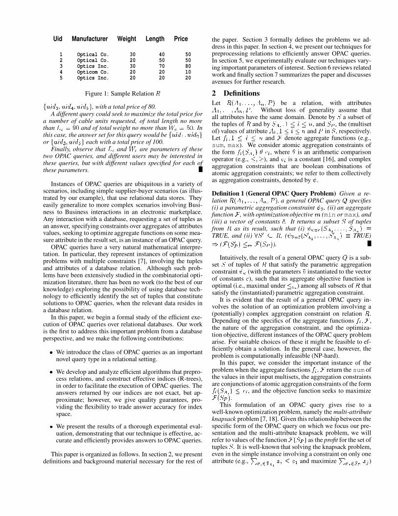
Example 2 Given the relation 4 in Table 1, the Pareto pointsare the round points in Figure 2. For example, (���� � �g� 3 is aPareto point with profit �� , realized by the entire set of tuples.

0 2 4 6 8 10 12 14 16 18 20 22 240

2

4

6

8

10

12

14

16

18

20

22

24

Query 1

Query 2

Figure 2: The Pareto set (round points), and an � -Pareto set(rectangular points) for the relation 4 .

The vector ( 9-���-9 3 with profit9 � is also a Pareto point, the

corresponding set of tuples being�X� # ��� & �

, because no vector( L # ��L � 3 withL # :h9.�

andL � :h9

has profit more than9 � .

The notion of Pareto sets are defined for arbitrary classesof constraint problems and functions, not only for the multi-attribute knapsack. The constraint problems can be discreteand, in most such cases, the Pareto set can have exponentiallymany elements. This happens because linear programs can beposed in the Pareto framework, and the convex hull of the so-lution space for linear programs can have exponentially many(in the number of objects/variables) vertices.

Relation S a1 a2 Profitt1 9 11 100t2 11 9 100t3 4 4 20

Table 1: Relation S

The size of the Pareto set for an instance of the multi-attribute knapsack problem can be exponential in the numberof tuples, even if the number of attributes is a small constant.Consider, for example, the case where there is only one at-tribute, * #

and a profit attribute2

, and tuple�

in relation �has the form ($� A � � A 3 . In this case, any subset of the tuples in� defines a unique cost and profit vector and no other set canachieve at least as small a cost and a higher profit. Therefore,all the subsets of tuples define dominating points.

To circumvent this problem, the concept of approximatingthe Pareto set has been introduced [14]. The � -Pareto set, is aset of “almost” optimal solutions defined as: for every optimalsolution

L, the � -Pareto set contains a solution that optimizes

each of the optimization criteria within a fraction of � . Theyalso show that the � -Pareto set for a multi-objective knapsackproblem can be computed efficiently and it is polynomial insize [14]. It is therefore a very powerful way to argue aboutapproximate solutions to multi-objective optimization prob-lems.

Given a relation � , functions D A and I , and � ~ , the � -

Pareto set, u1� is a set of solutions that almost dominate anyother solution.

Definition 3 ( � -Pareto set) The � -Pareto set for an OPACquery is a set of pairs

� (vVLg� 4 3�� of>

-dimensional vectorsVL � ( L.#��-,.,-,�L 0 3 and solutions 4 , such that, (a) there existsa solution 4\`B� with D A ($4 5 7 3S:qL A �-9;:B��:C>

, and (b) thereis no other pair (/VL ^ � 4_^ 3 , such that D.A�($4 {587 3�:�L {A �.9O:���:�>

,L {A : ( 9�� � 3vL A �.9K:q�8:q>and Ib(P� {� 3�~ ( 9S� � 3 Ib(P� � 3 .

Example 3 If we have � �� , � , the set of the rectangu-lar points in Figure 2 is an � -Pareto set. For example, point( 9-���-9 3 is in the � -Pareto set because there is no vector withcoordinates less than

9, � =� ( 9.���.9 3 that has profit more than9 � �� 9�, � .

The concept of an � -Pareto is very useful. Assuming thatthe size of this set is manageable, one could materialize it andseek to utilize it for query answering. Following the treatmentof [14] for � -Pareto sets, we can show the following:

Theorem 1 The size of the � -Pareto set for an OPAC query in-stance defined on a relation � is polynomial in � ��� (the size of� ) and

#� , but may be exponential in the number of attributes.

Proof: (Sketch) Assume that the>

attributes of � are integers.Since D A and I are polynomial functions (and more specifi-cally sums), the domain of each of these functions cannot bemore that ��� �8� for some constant � ~�9

. We can cover thespace of � 9� ��� �8� � with a set of geometrically increasing inter-vals with step

9�� � . To cover each domain we need �G(��p( � �8�� 3/3intervals (for some polynomial � ). Taking the Cartesian prod-uct we get a total of ��(��p( � �8�� 3 0 3 hyper-rectangles. Clearly,taking one solution from the interior of each hyper-rectangle(if such a solution exists) results in an � -Pareto set.

3 Problem StatementWe will provide the description of a technique suitable for ef-ficiently answering OPAC queries over a database. Our tech-nique will be approximate but will provide guarantees for itsaccuracy, and expose useful tradeoffs.

Assume for a moment that we had complete knowledge ofthe collection of OPAC queries one would be interested in.In that case, a straightforward approach could precompute theanswer of each query, assuming space was not an issue. In thatscenario, any query Q could be answered efficiently by usingthe vector of constants VL provided by Q to retrieve the cor-responding solution. Clearly, such a strategy is not feasiblebecause exact knowledge of queries is not commonly avail-able and the space overhead associated with such an approachcould be prohibitive.

Our solution is to preprocess relation � , constructing in-dex structures enabling efficient answers to arbitrary OPACqueries. For a query Q , we wish to provide either the exactanswer, or an answer that is guaranteed accurate, for suitablydefined notions of accuracy. Moreover, our construction willexpose a tradeoff between accuracy and space, providing theflexibility to fine tune the accuracy of our answers. We quan-tify the accuracy of answers to an OPAC query as follows:

Definition 4 ( � � ��{ -Accurate Answers) Let Q be an OPACquery specifying a vector of constants VL � ( L # �.,.,-,���L 0 3 , hav-ing an answer 4 with profit

2. For any � � � { ~

, an � � � { -Accurate answer to Q , is a vector VL { � ( L { # �-,.,.,/��L {0 3 and an

answer set 4 { , such that ] �v�-9a:�� :�>,L {A : ( 9K� � 3vL A and2 { ( 91� � { 3¡~H2

, where2 { is the profit of an OPAC query

specifying vector VL { of constants.

Assume that Q is a query specifying a vector VL of constantsand that the answer to Q is a set 4¢`C� with maximum profit2

. An � � � { -accurate answer to Q is an answer set 4 { that iseither the exact answer set 4 or it is an answer set correspond-ing to a query Q { . Query Q { specifies a vector of constantshaving values in each dimension less than or equal to

98� � ofthe corresponding values specified by Q . Moreover, the profitof Q { is strictly higher than a fraction of

9£� � { of2

. In thedefinition, without loss of generality, we assume the same �fraction is used for all constant values. Different values for �can be used for each of the values, if this is desirable, � beingdefined as a vector in this case. In fact, we do specify a dif-ferent approximation factor, ��^ , for the profit, to differentiatebetween the aggregate functions D and I .

We will preprocess relation � , constructing an index pro-viding � � � { -accurate answers to OPAC queries. Our prepro-cessing will consist of solving the multi-attribute knapsackproblem exactly, for a select subset of the candidate queryspace of all possible OPAC queries. We will then utilize thesesolutions towards providing � � � { -accurate answers to any can-didate OPAC query on � . This gives rise to the main problemwe address in the paper:

Problem 1 (Efficient OPAC Query Answering) Given arelation � , an OPAC query without the vector of constants ¤and � � � { , preprocess � constructing an index being able toefficiently provide � � � { -accurate answers to any OPAC queryon � that provides the parameters (values) to the constantvector ¤ .

Example 4 Consider the example of Figure 2 again. Assume� � �v^ �" , � . Assume that we are given the query ( 9 �.9-¥3 ,that is, find a set of objects that satisfy these conditions andmaximize the Profit. The set

�X� # �is an � � �v^ -accurate answer,

because it satisfies the constraints, and there is no other setthat has higher profit even if we relax the constraints by � .

If the query was ( 9 �.9 3 , the set�%� # �

is again an � � � ^ -accurate answer. Although the set does not satisfy the queryconstraints, it satisfies the relaxed constraints ( ( � �.9�9-3":9, � _� ( 9 �.9 3 ), and has the highest profit among all solutionsthat satisfy these constraints.

4 Efficient Answers to OPAC QueriesWe will now present our solutions and main technical resultsfor providing efficient answers to OPAC queries. We will de-scribe our approach in the following steps:' We will first present a technique to preprocess a rela-

tion � , evaluating solutions to a multi-attribute knapsackproblem on � , for only a select number of vectors ofconstants.' Following this preprocessing, we will then show how toutilize known indices (R-trees), to provide efficient � � � { -accurate answers to OPAC queries on � .' Finally, we will discuss issues related to the correctnessand completeness of our strategy.

4.1 Preprocessing �For a relation �O(P* # �.,-,., *10 ��2�3

, assume that the range of thei function applied on elements of each attribute *�A has range� ,.,.,§¦ � . 1.Any candidate query Q specifies an

>-dimensional vector

of constants VLC¨ � ,.,-,�¦ � 0 . We will preprocess the space� ,.,.,§¦ � 0 of all vectors of constants that can be specified bya possible query, creating a number of partitions that aim tocover the space of all possible queries. The partitions will beconstructed in a way such that, for all possible queries inside apartition, one can reason collectively about the properties andvalues of function I . Moreover, it will allow us to derive an� � � { -accurate answer for any query falling inside a partition.

We start by examining the relationship between the vec-tors of constants and the values of function I . We first definethe following property between

>-dimensional vectors of con-

stants:

Definition 5 Let VL � ( L.#��.,-,.,���L 0 3%� VL { � ( L { # �-,.,.,���L {0 3 be two>-dimensional vectors of constants. We say that VL is domi-

nated by VL { , ( VLK© VL { ) ifL A :CL {A �-9;:q�8:q>

.

We then make the following observation:

Observation 1 Let Q � Qª{ be two queries on � , specifyingvectors of constants VL�� VL { , having result sets 4 � 4 { respec-tively. If VL«© VL { then Id(+� � 3 � ikj-r l�m�s o�t : Ib(P� {� 3 �i j.r lgm {s ot .

Thus, if a vector of constants VL is dominated by a vector VL { , theprofit one can achieve for VL is less than or equal to the profitone can achieve using the vector VL { . A consequence of ob-servation 1 is the following: Consider a sequence of queries,with vectors of constants, VL # © VL � ,.,.,�© VL�e . Observing theevolution of the values of I in each answer obtained startingfrom VL¬e moving towards VL # , function I is monotonically nonincreasing. Our technique will trace the evolution of functionI along such sequences of dominated vectors. In order to beable to provide � � � { -accurate answers, one has to identify vec-tors of constants that cause the value of function I to changeby an � { fraction. At the same time, the coordinates of suchvectors have to be related by � as required by � � � { -accurateanswers.

Let � ,.,.,$¦ � 0 be the domain of all possible vectors of con-stants and consider one of these vectors, VLG¨ � ,.,.,§¦ � 0 . Let4 R� be the solution to the query with vector of constants VLand Id(�4 R� 3 be the associated profit. We will aim to identifythe vector of constants VL { by manipulating the coordinatesof vector VL by fractions of

91� � , such that (a) VL { © VL , (b)( 9p� � { 3 Ib($4 R� {3�~ Id(�4 R� 3 , where 4 R� { the solution to the OPAC

query with vector of constants VL { and (c) vector VL { is minimal.Consider the hyper rectangle defined by vectors VL { and VL . Bydefinition, any query with vector of constants inside the hyperrectangle has

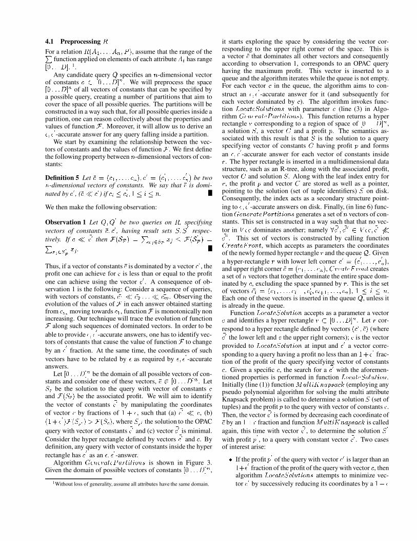
L { as an � � � { -answer.Algorithm ­�® > ®.¯�� � ® 2 ��¯ ���°���$±�>³² is shown in Figure 3.

Given the domain of possible vectors of constants � ,.,-,�¦ � 0 ,

1Without loss of generality, assume all attributes have the same domain.

it starts exploring the space by considering the vector cor-responding to the upper right corner of the space. This isa vector VL that dominates all other vectors and consequentlyaccording to observation 1, corresponds to an OPAC queryhaving the maximum profit. This vector is inserted to aqueue and the algorithm iterates while the queue is not empty.For each vector VL in the queue, the algorithm aims to con-struct an � � � { -accurate answer for it (and subsequently foreach vector dominated by VL ). The algorithm invokes func-tion

� ±�L � � ®.4 ±.´$������±�>³² with parameter VL (line (3) in Algo-rithm ­�® > ®-¯�� � ® 2 ��¯ ���µ����±�>³² ). This function returns a hyperrectangle ¯ corresponding to a region of space of � ,.,-,�¦ � 0 ,a solution 4 , a vector V¶ and a profit � . The semantics as-sociated with this result is that 4 is the solution to a queryspecifying vector of constants V¶ having profit � and formsan � � ��{ -accurate answer for each vector of constants inside¯ . The hyper rectangle is inserted in a multidimensional datastructure, such as an R-tree, along with the associated profit,vector V¶ and solution 4 . Along with the leaf index entry for¯ , the profit � and vector V¶ are stored as well as a pointer,pointing to the solution (set of tuple identifiers) 4 on disk.Consequently, the index acts as a secondary structure point-ing to � � ��{ -accurate answers on disk. Finally, (in line 6) func-tion ­ª® > ®.¯�� � ® 2 ��¯ ���°���$±�>³² generates a set of

>vectors of con-

stants. This set is constructed in a way such that that no vec-tor in · ® L dominates another; namely ] VL { � VL { { ¨ ·�® L�� VL {�¸©VL { { . This set of vectors is constructed by calling function¶ ¯�®-� � ®.¹�¯ ±�>�� , which accepts as parameters the coordinatesof the newly formed hyper rectangle ¯ and the queue ¤ . Givena hyper-rectangle ¯ with lower left corner VL { � ( L { # �-,.,.,/��L {0 3 ,and upper right corner VL � ( L #���,-,.,XL 0 3 , ¶ ¯�®-� � ®.¹�¯ ±�>�� createsa set of

>vectors that together dominate the entire space dom-

inated by VL , excluding the space spanned by ¯ . This is the setof vectors VL A � ( L.#��-,.,-,v��L A$º #-��L ^A ��L AP» # �.,-,.,/��L 0 3 , 9y:h��:¼>

.Each one of these vectors is inserted in the queue Q , unless itis already in the queue.

Function� ±�L � � ®-4 ±.´$�½����±�> accepts as a parameter a vectorVL and identifies a hyper rectangle ¯¡¾|� ,.,-,�¦ � 0 . Let ¯ cor-

respond to a hyper rectangle defined by vectors ( VL { � VL�3 (whereVL { the lower left and VL the upper right corners); VL is the vectorprovided to

� ±�L � � ®-4 ±.´$�½���$±�> at input and VL { a vector corre-sponding to a query having a profit no less than an

96� � { frac-tion of the profit of the query specifying vector of constantsVL . Given a specific VL , the search for a VL { with the aforemen-tioned properties is performed in function

� ±�L � � ®-4 ±.´$�½����±�> .Initially (line (1)) function ¿ ��´µ����À«> �.� ² � L � (employing anypseudo polynomial algorithm for solving the multi attributeKnapsack problem) is called to determine a solution 4 (set oftuples) and the profit � to the query with vector of constants VL .Then, the vector VL { is formed by decreasing each coordinate ofVL by an

9³� � fraction and function ¿ ��´µ���$Ày> �-� ² � L � is calledagain, this time with vector VL { , to determine the solution 4 {with profit � { , to a query with constant vector VL { . Two casesof interest arise:

' If the profit � { of the query with vector VL { is larger than an9 � ��{ fraction of the profit of the query with vector VL , thenalgorithm

� ±�L � � ®-4 ±.´$�½����±�>³² attempts to minimize vec-tor VL { by successively reducing its coordinates by a

9Á� �

Algorithm GeneratePartitions( ÂXõ { Ã/Ä )

Initialize:Q: Queue of multidimensional constraint vectorsÅ

: R-treeÆ Ã$Ç.Ã�Ç { : constraint vectorseach coordinate of Æ is initially set to beequal to Ä and, and Æ is added to Q

(1) while Q not empty(2) ÈÇ = headof(Q)(3) É$ʬà ÈË ÃµÌ�Ã/ͳΠ= LocateSolution( ÈÇ )(4) if there is no rectangle Ê%{ in the R-tree

Åthat contains rectangle Ê and Ê not NULL

(5) Insert É$ʬÃÏÌ�à ÈË Ã/ͳΠto the R-treeÅ

by storing É$Ê�ÃPÌ�à ÈË Î in a leaf index entryand maintaining a pointer to the set oftuple identifiers in the solution Í on disk

(6) CreateFront(Q,r)(7) endif(8) end-while

Algorithm LocateSolution( ÈÇ )Input: constant vector ÈÇ�ÐÑÉPÇ Ò/ÃXÓ�Ó�Ó�ÇXÔ�ÎOutput: É$Ê�à ÈË ÃµÌ�Ó Í³Î(1) (p,S) = MultiKnapsack( ÈÇ )(2) if (S is NULL) return (NULL, NULL, 0, NULL)(3) for i = 1 to n(4) ÇX{Õ�Ð×Ö 7Ò$Ø�Ù(5) ÉÚ̽{ÛÃ/ͳ{$Î = MultiKnapsack( ÈÇ { )(6) if ( ͳ{ is NULL) return (NULL, NULL, 0, NULL)(7) if ( É�ÜÁÝb { Î�Ì {³Þ Ì )(8) while (Ì {àß áÒ$Ø�Ù { )

(9) ÈÇXâ³Ð ÈÇ { ; ̽â³ÐaÌ { ; Í�â³ÐãÍ {(10) for i = 1 to n

(11) Ç {Õ Ð Ö { 7Ò$Ø�Ù {(12) (Ì { Ã/Í { ) = MultiKnapsack( ÈÇ { )(13) end-while(14) return (FormRect( ÈÇ%â , ÈÇ ), ÈÇXâ , ̽âvÃ/Í�â )(15) else(16) return (FormRect( ÈÇ { Ã�ÈÇ ), ÈÇ , Ì�ÃÛÍ )

Figure 3: Algorithm ­�® > ®.¯�� � ® 2 ��¯ ���°���$±�>³²

fraction, updating the solution 4 { and profit � { attainable(lines (5)-(12)). If it succeeds, the algorithm forms a hy-per rectangle using the minimal vector VL { and VL , returningit along with vector VL { , the profit � { and solution 4 { (line(14)) of VL { .' If, on the other hand, the profit of the query with vectorVL { is smaller than an

9K� �¬{ fraction of the profit of thequery with vector VL , then algorithm

� ±�L � � ®-4 ±.´$�½���$±�>³²does not attempt to reduce vector VL { further; it forms ahyper rectangle consisting of the ( VL { � VL�3 returning it alongwith the associated profit � , vector VL and solution 4 of VL(line (16)).

Function ¿ ��´°���$À«> �.� ² � L � with parameter VL is guaranteedto return a non empty solution, if a solution that satisfies theconstraints exists. The Function will return a null solutionif there is no subset of relation � satisfying the constraintsimposed by vector VL . To formalize this notion we define thefeasible region of relation � :

Definition 6 (Feasible Region) Let �)(+* # �.,-,., *;0 ��2ª3be a

relation with tuples (P* # �.,.,-, *10 3 . Assume that the i func-tion applied on elements of each attribute *�A and

2has range� ,.,.,§¦ � as well. The feasible region of � is the set of all vec-

tors VL dominated by vector ( ¦b�.,.,-,���¦G3, that dominate at least

one tuple of � .

Algorithm ­�® > ®-¯�� � ® 2 ��¯ ���µ����±�>³² progressively reduces thevalues in each dimension of vectors from the queue and even-tually vectors generated by

¶ ¯�®-� � ®.¹�¯ ±�>�� will be outside thefeasible region. As soon as a vector falls outside the feasi-ble region of � , function ¿ ��´µ����À«> �.� ² � L � returns null andprogressively the number of elements in the queue decreases.

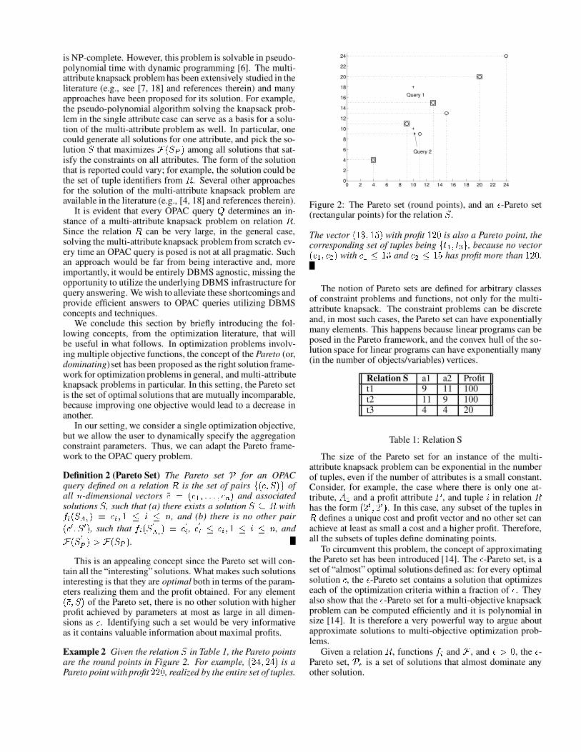
The following example illustrates the operation of the al-gorithm:

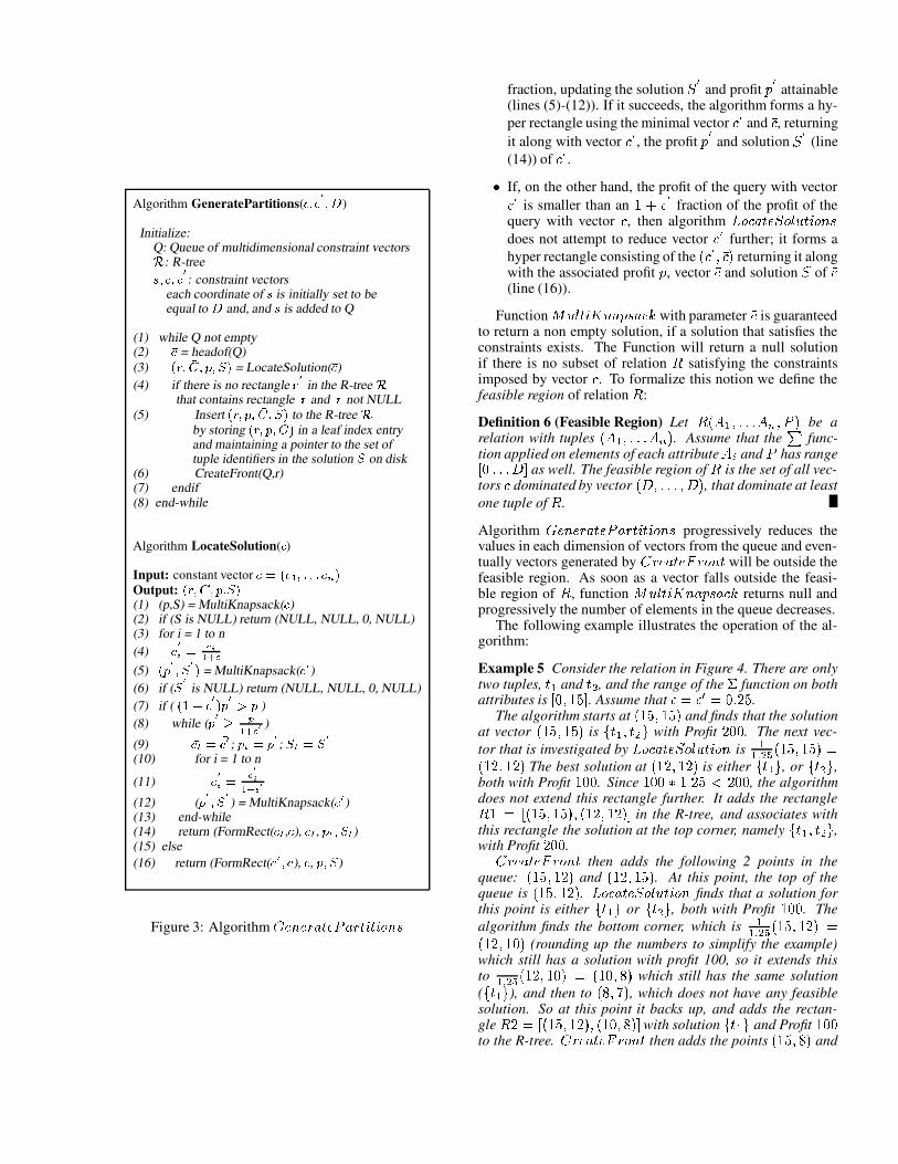
Example 5 Consider the relation in Figure 4. There are onlytwo tuples,

�%#and

���, and the range of the ä function on both

attributes is � �-9 � . Assume that � � ��^ �< , � .The algorithm starts at ( 9 �-9 3 and finds that the solution

at vector ( 9 �-9 3 is�%� # ��� � �

with Profit � . The next vec-tor that is investigated by

� ±�L � � ®.4 ±.´$������±�> is##�å ��� ( 9 �-9 3 �( 9 � �-9 � 3 The best solution at ( 9 � �.9 � 3 is either�X�-#X�

, or�X���g�

,both with Profit

9 . Since

9 � � 9, � aæ � � , the algorithmdoes not extend this rectangle further. It adds the rectangle� 9 � �Ï( 9 �-9 3X� ( 9 � �.9 � 3 � in the R-tree, and associates withthis rectangle the solution at the top corner, namely

�X�.# ����.�,

with Profit � .¶ ¯�®-� � ®.¹�¯ ±�>�� then adds the following 2 points in thequeue: ( 9 �.9 � 3 and ( 9 � �.9 3 . At this point, the top of thequeue is ( 9 �.9 � 3 . � ±�L � � ®-4 ±.´$�½����±�> finds that a solution forthis point is either

�X� # �or

�%� � �, both with Profit

9 . The

algorithm finds the bottom corner, which is##�å ��� ( 9 �.9 � 3 �

( 9 � �-9 3 (rounding up the numbers to simplify the example)which still has a solution with profit 100, so it extends thisto

##�å ��� ( 9 � �.9 3 � ( 9 ��¥3 which still has the same solution(�X�X#%�

), and then to ( ¥���ç�3 , which does not have any feasiblesolution. So at this point it backs up, and adds the rectan-gle ��� � �µ( 9 �.9 � 3X� ( 9 ��¥3 � with solution

�X�%#X�and Profit

9 to the R-tree.

¶ ¯�®-� � ®.¹�¯ ±�>�� then adds the points ( 9 ��¥�3 and

(15,15)(15,12)(12,15)

(12,15)(15,8)(10,12)

(15,8)(10,12)(12,10)(8,15)

(10,12)(12,10)(8,15)(15,6)(10,8)

(12,10)(8,15)(15,6)(10,8)(8,12)(10,10)

R1 R2 R3 R4

CONTENTS OF QUEUE:

5 10 100 (t2) 10 5 100 (t1) 15 15 200 (t1, t2)

c1 c2 P Solution

t1 10 5 100 t2 5 10 100

c1 c2 Profit

DATABASE

RESULT FOR c1 & c2 <=15

EXAMPLE LEAF ENTRY

R1 Profit=200 Sol. .

0 5 10 150

5

10

15R1

R2

R3

R4

... until queue is empty

Figure 4: The operation of algorithm ­�® > ®.¯�� � ® 2 ��¯ ���°����±�>³²

1000 2000 3000 4000 5000 6000 7000 8000 9000 100001000

2000

3000

4000

5000

6000

7000

8000

9000

10000Index: Gaussian ε=0.1, ε’=0.1

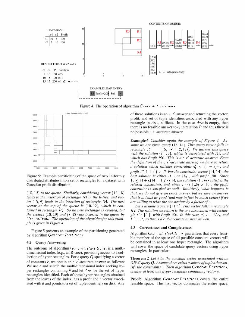
Figure 5: Example partitioning of the space of two uniformlydistributed attributes into a set of rectangles for a dataset withGaussian profit distribution.

( 9 �-9 � 3 to the queue. Similarly, considering vector ( 9 � �-9 3leads to the insertion of rectangle � �

in the R-tree, and vec-tor ( 9 ��¥3 leads to the insertion of rectangle �;� . The nextvector at the top of the queue is ( 9 �.9 � 3 , which is con-tained in rectangle � �

. So no new rectangle is created, butthe vectors ( 9 �-9 3 and ( ¥��.9 � 3 are inserted in the queue by¶ ¯�®-� � ®.¹�¯ ±�>�� . The operation of the algorithm for this exam-ple is given in Figure 4.

Figure 5 presents an example of the partitioning generatedby algorithm ­ª® > ®.¯�� � ® 2 ��¯ ���°���$±�>³² .4.2 Query AnsweringThe outcome of algorithm ­�® > ®-¯�� � ® 2 ��¯ ���µ����±�>³² , is a multi-dimensional index (e.g., an R-tree), providing access to a col-lection of hyper rectangles. For a query Q specifying a vectorof constants VL , we obtain an � � � { -accurate answer as follows:We use VL and search the multidimensional index seeking hy-per rectangles containing VL and let * >³²

be the set of hyperrectangles identified. Each of these hyper rectangles obtainedfrom the leaves of the index, has a profit and a vector associ-ated with it and points to a set of tuple identifiers on disk. Any

of these solutions is an � � � { answer and returning the vector,profit, and set of tuple identifiers associated with any hyperrectangle in * >³²

, suffices. In the case * >³²is empty, then

there is no feasible answer to Q in relation � and thus there isno possible � � �¬{ -accurate answer.

Example 6 Consider again the example of Figure 4. As-sume we are given query ( 9 � �-9 � 3 . This query vector falls inrectangle � 9 � �µ( 9 �-9 3%� ( 9 � �.9 � 3 � . We answer this querywith the solution

�X�%#������.�, which is associated with � 9

, andwhich has Profit � � . This is a � � ��^ -accurate answer: Fromthe definition of the � � ��^ -accurate answer, we have to returna solution which satisfies constraints

L ^A æ ( 9�� � 3/L A � andprofit

2 ^�( 9£� � { 3K~!2K,For the constraint vector ( 9 � �.9 � 3 , the

best solution is either�X� # �

or�%� � �

, with profit9

. Since9 : ( 9Á� � 3%9 � � 9, � K� 9 � , the solution�X� # �Û� � �

satisfies therelaxed constraints, and, since � �ª� 9�, � ~H9

, the profitconstraint is satisfied as well. Intuitively, what happens isthat, we do not give an exact answer, but we give an answerthat is at least as good (and may in fact be much better) if weare willing to relax the constraints by a factor of � .

Let’s assume a query ( 9 � � � 3 . This vector falls in rectangle��� . The solution we return is the one associated with rectan-gle ¯�� :

�%� # �, with Profit

9 �. In this case,

L ^A æ 9�, � L A , and2 ^ � 2, so this is a � � �v^ -accurate answer as well.

4.3 Correctness and CompletenessAlgorithm ­�® > ®.¯�� � ® 2 ��¯ ���°����±�>³² guarantees that every feasi-ble member of the space of all possible constant vectors willbe contained in at least one hyper rectangle. The algorithmwill cover the space of candidate query vectors using hyperrectangles. In particular:

Theorem 2 Let VL be the constant vector associated with anOPAC query Q . Assume there exists a subset of tuples that sat-isfy the constraints VL . Then algorithm ­�® > ®-¯�� � ® 2 ��¯ ���µ����±�>³² ,creates at least one hyper rectangle containing vector VL .Proof: Algorithm ­�® > ®-¯�� � ® 2 ��¯ ���µ����±�>³² covers the entirefeasible space: The first vector dominates the entire space.

Each iteration of the algorithm takes a vector from the queue,uses this vector to form the upper right corner of a new hyperrectangle, and adds a new set of vectors in the queue that to-gether dominate the space that the original vector dominatedwith the exception of the space of the hyper-rectangle. Sincethe algorithm terminates when no vectors are in the queue,it follows that the entire feasible space is covered by hyper-rectangles.

The following result demonstrates that the answer to anyOPAC query, Q , specifying a vector of constants VL , obtainedfrom the index, is an � � � { -accurate answer.

Theorem 3 Let Q be a query specifying vector VL as a con-stant vector. Let ¯ be a hyper rectangle containing VL , gener-ated by algorithm ­�® > ®.¯�� � ® 2 ��¯ ���°����±�>³² . The answer to Qreturned from the index, consisting of a vector, a set of tuples,and a profit is an � � � { -accurate answer.

Proof: Let � � be the profit of the lower left corner vectorVL%� , and � # be the profit of the upper right corner vector VL�#of multidimensional rectangle ¯ . Assume a vector VL locatedinside ¯ .

If � � ( 9K� ��{ 3GM � # , then the lower left corner is an � � �¬{ -accurate answer: since VL � is dominated by VL # , the optimalprofit for VL is at most � # , and therefore at most an

9.� � { fractionhigher than � � . In this case algorithm ­ª® > ®.¯�� � ® 2 ��¯ ���°���$±�>³²stores in the index entry, along with ¯ , a vector with coordi-nates equal to VL � and a profit � � and thus the answer returnedis an � � ��{ -accurate answer.

If on the other hand � � ( 91� � { 3 æ � # , then the profit ofthe lower left corner may be more than a fraction of

9K� �X{smaller than the profit of the query. However, by the con-struction of the algorithm ­�® > ®.¯�� � ® 2 ��¯ ���°���$±�>³² this can onlyhappen if all the values of the vector VL are within an

91� �fraction of the values of the upper right vector VL # . In this case,VL # provides an � � � { -accurate answer since it gives a much bet-ter profit with just an � relaxation of the constraints. Algo-rithm ­�® > ®-¯�� � ® 2 ��¯ ���µ����±�>³² will associate the vector VL�# andits profit with the index entry, along with ¯ .

Restricting our attention to monotone classes of aggrega-tion functions, we can improve the computational aspects re-lated to the construction of an � -Pareto set. The followingtheorem shows that the total number of hyper-rectangles rep-resented in our index is polynomial.

Theorem 4 The number of vectors that create new multidi-mensional rectangles at any step of the execution of algorithmGeneratePartitions, is polynomial to

#� .

Proof: Assume that the range of the ä function applied onthe * A attribute values of a non-empty subset of the tuples is� 9�,.,.,§¦ � for each

�. Here we assume that the attributes have

non zero values; to deal with zero values we have to add theinterval from zero to the smallest non zero value as one addi-tional interval in the partition.

Then we can partition the range in �G(qè é�ê�ëè é�ê-ì# » ��í 3 � �G(Xè é�ê�ë� 3

intervals (for�æ � æ 9.3

, geometrically increasing with step9�� � . Taking the Cartesian product of the>

attributes, we cre-ate �G(v( è é�ê�ë� 3 0 3=> dimensional points. Note that, by the con-struction of the algorithm, every vector inserted in the queue

corresponds to one of these points. It follows that the numberof hyper rectangles in the index is polynomial to

9-î � and tothe size of the range of the ä function applied on the attributevalues, and is exponential to the number of the attributes.

In section 5 we will experimentally evaluate the effectsdata distribution has on the execution time of algorithm­ª® > ®.¯�� � ® 2 ��¯ ���°���$±�>³² .5 Experimental EvaluationIn this section we present the results of a comprehensive set ofexperiments, aiming to experimentally investigate the proper-ties of algorithm ­�® > ®.¯�� � ® 2 ��¯ ���°���$±�>³² . We seek to quantifythe tradeoffs in terms of construction time and accuracy of ourproposed techniques.

In our experiments we evaluate the impact of the pa-rameters � and � { on the execution time of algorithm­ª® > ®.¯�� � ® 2 ��¯ ���°���$±�>³² . We present scalability experiments,varying the number of tuples of the underlying relation, thesizes of the attribute domains and the number of attributes (di-mensionality of the problem). We experimentally evaluate theaccuracy of our approach. Finally we experimentally evalu-ate the efficiency of the technique, measuring the size of theindex, and the query response time. All experiments were per-formed on an Athlon 1.3Ghz with 1Gb of memory and 60GBdisk space.

5.1 Description of datasetsOur experimental test bed includes datasets with three distinctdistributions in the profit attribute, namely Uniform, Gaussianand Zipfian. The rest of the attributes ( * # ,.,-,�� *10 ) on whichconstraints are posed are independently and normally dis-tributed. We vary the number of these attributes from two (2Ddata sets) to three (3D data sets), effectively constructing threeand four dimensional data spaces. For each profit attributedistributionwe tested, we also produced data sets, introducingcorrelations between the attributes * #8,-,., * 0 . For correlatedattributes the correlation coefficient ranged between 0.7-0.8.Therefore, we had at our disposal a large collection of diversedatasets, that helped us understand and quantify the effect ofthe various parameters on the performance of our techniques.

5.2 Index construction timeWith this set of experiments, we evaluate the impact of theparameters � and � { , the dataset distribution, attribute corre-lation, and dataset size on the total index construction time.This time consists of two distinct components:

' MultiKnapsack Execution Time. This is the total timerequired by all invocations to the MultiKnapsack func-tion in algorithm ­�® > ®.¯�� � ® 2 ��¯ ���°����±�>³² . This time de-pends on the distributional characteristics of the data setsand their dimensionality.

' Partition Generation Time. It includes the time re-quired to cover the domain space with hyper-rectanglesof solutions. This step is directly affected by the param-eters � and � { , as well as the dimensionality of the under-lying data space.

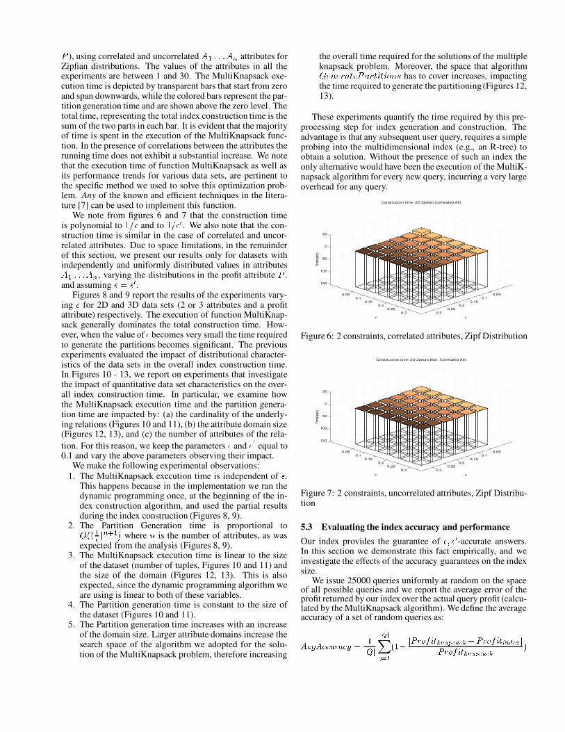
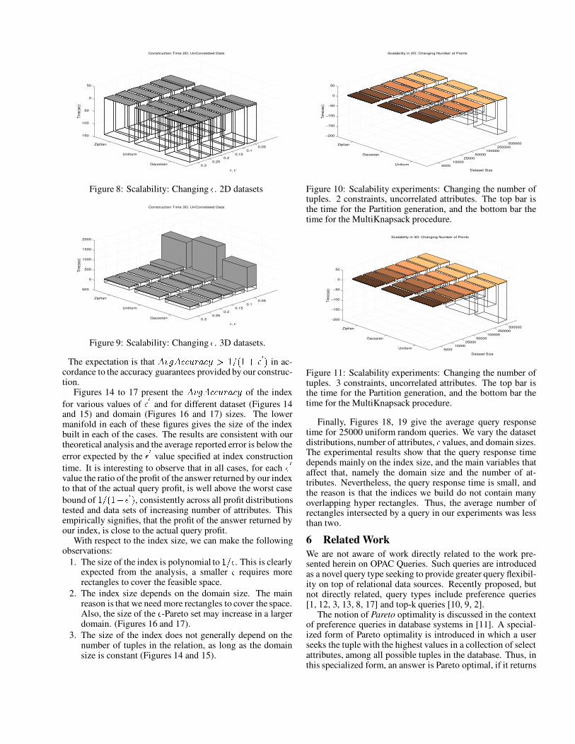
Figures 6 and 7 report the total index construction time forthe 2D datasets (two attributes * #-� * �

and a profit attribute

2), using correlated and uncorrelated * # ,-,., *10 attributes for

Zipfian distributions. The values of the attributes in all theexperiments are between 1 and 30. The MultiKnapsack exe-cution time is depicted by transparent bars that start from zeroand span downwards, while the colored bars represent the par-tition generation time and are shown above the zero level. Thetotal time, representing the total index construction time is thesum of the two parts in each bar. It is evident that the majorityof time is spent in the execution of the MultiKnapsack func-tion. In the presence of correlations between the attributes therunning time does not exhibit a substantial increase. We notethat the execution time of function MultiKnapsack as well asits performance trends for various data sets, are pertinent tothe specific method we used to solve this optimization prob-lem. Any of the known and efficient techniques in the litera-ture [7] can be used to implement this function.

We note from figures 6 and 7 that the construction timeis polynomial to

9.î � and to9-î ��^ . We also note that the con-

struction time is similar in the case of correlated and uncor-related attributes. Due to space limitations, in the remainderof this section, we present our results only for datasets withindependently and uniformly distributed values in attributes* #Á,.,-, * 0 , varying the distributions in the profit attribute

2.

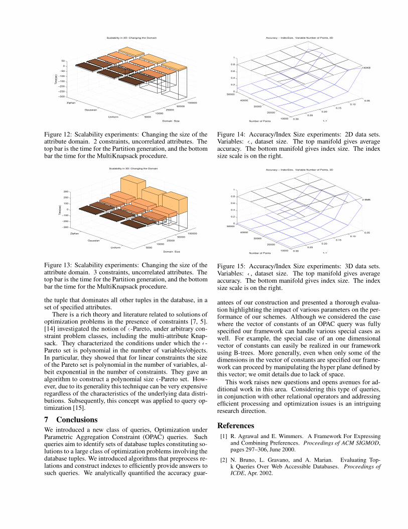
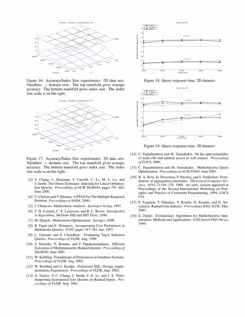
and assuming � � �v^ .Figures 8 and 9 report the results of the experiments vary-

ing � for 2D and 3D data sets (2 or 3 attributes and a profitattribute) respectively. The execution of function MultiKnap-sack generally dominates the total construction time. How-ever, when the value of � becomes very small the time requiredto generate the partitions becomes significant. The previousexperiments evaluated the impact of distributional character-istics of the data sets in the overall index construction time.In Figures 10 - 13, we report on experiments that investigatethe impact of quantitative data set characteristics on the over-all index construction time. In particular, we examine howthe MultiKnapsack execution time and the partition genera-tion time are impacted by: (a) the cardinality of the underly-ing relations (Figures 10 and 11), (b) the attribute domain size(Figures 12, 13), and (c) the number of attributes of the rela-tion. For this reason, we keep the parameters � and � { equal to0.1 and vary the above parameters observing their impact.

We make the following experimental observations:1. The MultiKnapsack execution time is independent of � .

This happens because in the implementation we ran thedynamic programming once, at the beginning of the in-dex construction algorithm, and used the partial resultsduring the index construction (Figures 8, 9).

2. The Partition Generation time is proportional to�G(/( #� 3 0�»# 3

where>

is the number of attributes, as wasexpected from the analysis (Figures 8, 9).

3. The MultiKnapsack execution time is linear to the sizeof the dataset (number of tuples, Figures 10 and 11) andthe size of the domain (Figures 12, 13). This is alsoexpected, since the dynamic programming algorithm weare using is linear to both of these variables.

4. The Partition generation time is constant to the size ofthe dataset (Figures 10 and 11).

5. The Partition generation time increases with an increaseof the domain size. Larger attribute domains increase thesearch space of the algorithm we adopted for the solu-tion of the MultiKnapsack problem, therefore increasing

the overall time required for the solutions of the multipleknapsack problem. Moreover, the space that algorithm­�® > ®.¯�� � ® 2 ��¯ ���°����±�>³² has to cover increases, impactingthe time required to generate the partitioning(Figures 12,13).

These experiments quantify the time required by this pre-processing step for index generation and construction. Theadvantage is that any subsequent user query, requires a simpleprobing into the multidimensional index (e.g., an R-tree) toobtain a solution. Without the presence of such an index theonly alternative would have been the execution of the MultiK-napsack algorithm for every new query, incurring a very largeoverhead for any query.

0.30.25

0.20.15

0.10.05

0.30.25

0.20.15

0.10.05

150

100

50

0

50

ε

Construction time: 2D Zipfian,Correlated Attr.

ε’Ti

me(

sec)

Figure 6: 2 constraints, correlated attributes, Zipf Distribution

0.30.25

0.20.15

0.10.05

0.30.25

0.20.15

0.10.05

150

100

50

0

50

ε

Construction time: 2D Zipfian,Non−Correlated Attr.

ε’

Tim

e(se

c)

Figure 7: 2 constraints, uncorrelated attributes, Zipf Distribu-tion

5.3 Evaluating the index accuracy and performanceOur index provides the guarantee of � � ��^ -accurate answers.In this section we demonstrate this fact empirically, and weinvestigate the effects of the accuracy guarantees on the indexsize.

We issue 25000 queries uniformly at random on the spaceof all possible queries and we report the average error of theprofit returned by our index over the actual query profit (calcu-lated by the MultiKnapsack algorithm). We define the averageaccuracy of a set of random queries as:

ïKð%ñ�ï Ç�ÇXò�Ê�ó�ÇXô1Ð Üõ ö�õ÷ ø³÷ùú�û Ò É�Ü�ü

õ ý Ê�þ�ÿ������ Ô�� á� � Ö �8ü ý Ê�þ�ÿ���� Õ Ô���� õý Ê�þ ÿ������ Ô�� á� � Ö � Î

0.30.25

0.20.15

0.10.05

Gaussian

Uniform

Zipfian

150

100

50

0

50

ε, ε’

Construction Time 2D, UnCorrelated Data

Tim

e(se

c)

Figure 8: Scalability: Changing � . 2D datasets

0.30.25

0.20.15

0.10.05

Gaussian

Uniform

Zipfian

500

0

500

1000

1500

2000

ε, ε’

Construction Time 3D, UnCorrelated Data

Tim

e(se

c)

Figure 9: Scalability: Changing � . 3D datasets.

The expectation is that * f�� * LXLX� ¯�� L��E~}9-î ( 9£� �¬{ 3 in ac-cordance to the accuracy guarantees provided by our construc-tion.

Figures 14 to 17 present the * f�� * LXLX� ¯�� L�� of the indexfor various values of � { and for different dataset (Figures 14and 15) and domain (Figures 16 and 17) sizes. The lowermanifold in each of these figures gives the size of the indexbuilt in each of the cases. The results are consistent with ourtheoretical analysis and the average reported error is below theerror expected by the �¬{ value specified at index constructiontime. It is interesting to observe that in all cases, for each �X{value the ratio of the profit of the answer returned by our indexto that of the actual query profit, is well above the worst casebound of

9-î ( 9�� � { 3 , consistently across all profit distributionstested and data sets of increasing number of attributes. Thisempirically signifies, that the profit of the answer returned byour index, is close to the actual query profit.

With respect to the index size, we can make the followingobservations:

1. The size of the index is polynomial to9.î � . This is clearly

expected from the analysis, a smaller � requires morerectangles to cover the feasible space.

2. The index size depends on the domain size. The mainreason is that we need more rectangles to cover the space.Also, the size of the � -Pareto set may increase in a largerdomain. (Figures 16 and 17).

3. The size of the index does not generally depend on thenumber of tuples in the relation, as long as the domainsize is constant (Figures 14 and 15).

500010000

2500050000

100000250000

500000

Uniform

Gaussian

Zipfian

−200

−150

−100

−50

0

50

Dataset Size

Scalability in 2D: Changing Number of Points

Tim

e(se

c)

Figure 10: Scalability experiments: Changing the number oftuples. 2 constraints, uncorrelated attributes. The top bar isthe time for the Partition generation, and the bottom bar thetime for the MultiKnapsack procedure.

500010000

2500050000

100000250000

500000

Uniform

Gaussian

Zipfian

−200

−150

−100

−50

0

50

Dataset Size

Scalability in 3D: Changing Number of Points

Tim

e(se

c)

Figure 11: Scalability experiments: Changing the number oftuples. 3 constraints, uncorrelated attributes. The top bar isthe time for the Partition generation, and the bottom bar thetime for the MultiKnapsack procedure.

Finally, Figures 18, 19 give the average query responsetime for 25000 uniform random queries. We vary the datasetdistributions, number of attributes, � values, and domain sizes.The experimental results show that the query response timedepends mainly on the index size, and the main variables thataffect that, namely the domain size and the number of at-tributes. Nevertheless, the query response time is small, andthe reason is that the indices we build do not contain manyoverlapping hyper rectangles. Thus, the average number ofrectangles intersected by a query in our experiments was lessthan two.

6 Related WorkWe are not aware of work directly related to the work pre-sented herein on OPAC Queries. Such queries are introducedas a novel query type seeking to provide greater query flexibil-ity on top of relational data sources. Recently proposed, butnot directly related, query types include preference queries[1, 12, 3, 13, 8, 17] and top-k queries [10, 9, 2].

The notion of Pareto optimality is discussed in the contextof preference queries in database systems in [11]. A special-ized form of Pareto optimality is introduced in which a userseeks the tuple with the highest values in a collection of selectattributes, among all possible tuples in the database. Thus, inthis specialized form, an answer is Pareto optimal, if it returns

5000

10000

25000

50000

100000

Uniform

Gaussian

Zipfian

−300

−250

−200

−150

−100

−50

0

50

Domain Size

Scalability in 2D: Changing the Domain

Tim

e(se

c)

Figure 12: Scalability experiments: Changing the size of theattribute domain. 2 constraints, uncorrelated attributes. Thetop bar is the time for the Partition generation, and the bottombar the time for the MultiKnapsack procedure.

5000

10000

25000

50000

100000

Uniform

Gaussian

Zipfian

−300

−200

−100

0

100

200

300

Domain Size

Scalability in 3D: Changing the Domain

Tim

e(se

c)

Figure 13: Scalability experiments: Changing the size of theattribute domain. 3 constraints, uncorrelated attributes. Thetop bar is the time for the Partition generation, and the bottombar the time for the MultiKnapsack procedure.

the tuple that dominates all other tuples in the database, in aset of specified attributes.

There is a rich theory and literature related to solutions ofoptimization problems in the presence of constraints [7, 5].[14] investigated the notion of � -Pareto, under arbitrary con-straint problem classes, including the multi-attribute Knap-sack. They characterized the conditions under which the � -Pareto set is polynomial in the number of variables/objects.In particular, they showed that for linear constraints the sizeof the Pareto set is polynomial in the number of variables, al-beit exponential in the number of constraints. They gave analgorithm to construct a polynomial size � -Pareto set. How-ever, due to its generality this technique can be very expensiveregardless of the characteristics of the underlying data distri-butions. Subsequently, this concept was applied to query op-timization [15].

7 ConclusionsWe introduced a new class of queries, Optimization underParametric Aggregation Constraint (OPAC) queries. Suchqueries aim to identify sets of database tuples constituting so-lutions to a large class of optimization problems involving thedatabase tuples. We introduced algorithms that preprocess re-lations and construct indexes to efficiently provide answers tosuch queries. We analytically quantified the accuracy guar-

10000

20000

30000

40000

50000

0.05

140KB

0.10

0.15

0.20

0.25

0.30

0

0.2

0.4

0.6

0.8

1

ε, ε’

Accuracy − IndexSize, Variable Number of Points, 2D

Number of Points

Figure 14: Accuracy/Index Size experiments: 2D data sets.Variables: � , dataset size. The top manifold gives averageaccuracy. The bottom manifold gives index size. The indexsize scale is on the right.

10000

20000

30000

40000

50000

0.05

2.9MB

0.10

0.15

0.20

0.25

0.30

0

0.2

0.4

0.6

0.8

1

ε, ε’

Accuracy − IndexSize, Variable Number of Points, 3D

Number of Points

Figure 15: Accuracy/Index Size experiments: 3D data sets.Variables: � , dataset size. The top manifold gives averageaccuracy. The bottom manifold gives index size. The indexsize scale is on the right.

antees of our construction and presented a thorough evalua-tion highlighting the impact of various parameters on the per-formance of our schemes. Although we considered the casewhere the vector of constants of an OPAC query was fullyspecified our framework can handle various special cases aswell. For example, the special case of an one dimensionalvector of constants can easily be realized in our frameworkusing B-trees. More generally, even when only some of thedimensions in the vector of constants are specified our frame-work can proceed by manipulating the hyper plane defined bythis vector; we omit details due to lack of space.

This work raises new questions and opens avenues for ad-ditional work in this area. Considering this type of queries,in conjunction with other relational operators and addressingefficient processing and optimization issues is an intriguingresearch direction.

References[1] R. Agrawal and E. Wimmers. A Framework For Expressing

and Combining Preferences. Proceedings of ACM SIGMOD,pages 297–306, June 2000.

[2] N. Bruno, L. Gravano, and A. Marian. Evaluating Top-k Queries Over Web Accessible Databases. Proceedings ofICDE, Apr. 2002.

10000

20000

30000

40000

50000

0.05

112KB

0.10

0.15

0.20

0.25

0.30

0

0.2

0.4

0.6

0.8

1

ε, ε’

Accuracy − IndexSize, Variable Domain, 2D

Domain

Figure 16: Accuracy/Index Size experiments: 2D data sets.Variables: � , domain size. The top manifold gives averageaccuracy. The bottom manifold gives index size. The indexsize scale is on the right.

10000

20000

30000

40000

50000

0.05

4.6MB

0.10

0.15

0.20

0.25

0.30

0

0.2

0.4

0.6

0.8

1

ε, ε’

Accuracy − IndexSize, Variable Domain, 3D

Domain

Figure 17: Accuracy/Index Size experiments: 3D data sets.Variables: � , domain size. The top manifold gives averageaccuracy. The bottom manifold gives index size. The indexsize scale is on the right.

[3] Y. Chang, L. Bergman, V. Castelli, C. Li, M. L. Lo, andJ. Smith. The Onion Technique: Indexing for Linear Optimiza-tion Queries. Proceedings of ACM SIGMOD, pages 391–402,June 2000.

[4] C. Chekuri and S. Khanna. A PTAS For The Multiple KnapsackProblem. Proceedings of SODA, 2000.

[5] J. Climacao. Multicriteria Analysis. Sprienger Verlag, 1997.[6] T. H. Cormen, C. E. Leiserson, and R. L. Rivest. Introduction

to Algorithms. McGraw Hill and MIT Press, 1990.[7] M. Ehrgott. Multicriteria Optimization. Springer, 2000.[8] R. Fagin and E. Wimmers. Incorporating User Preferences in

Multimedia Queries. ICDT, pages 247–261, Jan. 1997.[9] L. Gravano and S. Chaudhuri. Evaluating Top-k Selection

Queries. Proceedings of VLDB, Aug. 1999.[10] V. Hristidis, N. Koudas, and Y. Papakonstantinou. Efficient

Execution of Multiparametric Ranked Queries. Proceedings ofSIGMOD, June 2001.

[11] W. Kiebling. Foundations of Preferences in Database Systems.Proceedings of VLDB, Aug. 2002.

[12] W. Kiebling and G. Kostler. Preference SQL: Design, Imple-mentation, Experiences. Proceedings of VLDB, Aug. 2002.

[13] A. Natsev, Y.-C. Chang, J. Smith, C.-S. Li, and J. S. Vitter.Supporting Incremental Join Queries on Ranked Inputs. Pro-ceedings of VLDB, Aug. 2001.

10000 20000 30000 40000 500000

0.2

0.4

0.6

0.8

1

Inde

x Res

pons

e Ti

me

for 5

000

quer

ies (s

ec)

Domain Size

ε=ε’=0.1

0

0.2

0.4

0.6

0.8

1

ε=ε’=0.3

Query Time 2D

UniformGaussianZipfian

Figure 18: Query response time, 2D datasets

10000 20000 30000 40000 500000

0.2

0.4

0.6

0.8

1

Inde

x Res

pons

e Ti

me

for 5

000

quer

ies (s

ec)

Domain Size

ε=ε’=0.1

0

0.2

0.4

0.6

0.8

1

ε=ε’=0.3

Query Time 3D

UniformGaussianZipfian

Figure 19: Query response time, 3D datasets

[14] C. Papadimitriou and M. Yannakakis. On the approximabilityof trade-offs and optimal access to web sources. Proceedingsof FOCS, 2000.

[15] C. Papadimitriou and M. Yannakakis. Multiobjective QueryOptimization. Proceedings of ACM PODS, June 2001.

[16] K. A. Ross, D. Srivastava, P. Stuckey, and S. Sudarshan. Foun-dations of aggregation constraints. Theoretical Computer Sci-ence, 193(1-2):149–179, 1998. An early version appeared inProceedings of the Second International Workshop on Prin-ciples and Practice of Constraint Programming, 1994, LNCS874.

[17] P. Tsaparas, T. Palpanas, Y. Kotidis, N. Koudas, and D. Sri-vastava. Ranked Join Indicies. Proceedings IEEE ICDE, Mar.2003.

[18] E. Zitzler. Evolutionary Algorithms for Multiobjective Opti-mization: Methods and Applications. ETH Zurich PhD Thesis,1999.