www.elsevier.com/locate/jim
Journal of Immunological Methods 290 (2004) 93–105
Review
Automated interpretation of subcellular patterns from
immunofluorescence microscopy
Yanhua Hua, Robert F. Murphya,b,c,*
aDepartment of Biological Sciences, Carnegie Mellon University, 4400 Fifth Avenue, Pittsburgh, PA 15213, USAbDepartment of Biomedical Engineering, Carnegie Mellon University, 4400 Fifth Avenue, Pittsburgh, PA 15213, USA
cCenter for Automated Learning and Discovery, Carnegie Mellon University, 4400 Fifth Avenue, Pittsburgh, PA 15213, USA
Accepted 8 April 2004
Available online 28 May 2004
Abstract
Immunofluorescence microscopy is widely used to analyze the subcellular locations of proteins, but current approaches rely
on visual interpretation of the resulting patterns. To facilitate more rapid, objective, and sensitive analysis, computer programs
have been developed that can identify and compare protein subcellular locations from fluorescence microscope images. The
basis of these programs is a set of features that numerically describe the characteristics of protein images. Supervised machine
learning methods can be used to learn from the features of training images and make predictions of protein location for images
not used for training. Using image databases covering all major organelles in HeLa cells, these programs can achieve over 92%
accuracy for two-dimensional (2D) images and over 95% for three-dimensional images. Importantly, the programs can
discriminate proteins that could not be distinguished by visual examination. In addition, the features can also be used to
rigorously compare two sets of images (e.g., images of a protein in the presence and absence of a drug) and to automatically
select the most typical image from a set. The programs described provide an important set of tools for those using fluorescence
microscopy to study protein location.
D 2004 Elsevier B.V. All rights reserved.
Keywords: (3–6) Fluorescence microscopy; Subcellular location features; Pattern recognition; Location proteomics
1. Introduction
0022-1759/$ - see front matter D 2004 Elsevier B.V. All rights reserved.
doi:10.1016/j.jim.2004.04.011
Abbreviations: COF, center of fluorescence; CHO, Chinese
hamster ovary; SDA, Stepwise Discriminant Analysis; SLF,
subcellular location features; 2D, two-dimensional; 3D, three-
dimensional.
* Corresponding author. Departments of Biological Sciences
and Biomedical Engineering, Center for Automated Learning and
Discovery, Carnegie Mellon University, 4400 Fifth Avenue,
Pittsburgh, PA 15213, USA. Tel.: +1-412-268-3480; fax: +1-412-
268-6571.
E-mail address: [email protected] (R.F. Murphy).
Detailed knowledge of the subcellular location of a
protein is critical to a complete understanding of its
function. Fluorescence microscopy, especially immu-
nofluorescence microscopy, is widely used by cell
biologists to localize proteins to specific organelles or
to observe the colocalization of two or more proteins
(see Miller and Shakes, 1995; Brelie et al., 2002 for
reviews of sample preparation and imaging methods).
It is also frequently used to study changes in subcel-
lular location due to drug effects or resulting from
Y. Hu, R.F. Murphy / Journal of Immunological Methods 290 (2004) 93–10594
development, mutation, or disease. Traditionally, vi-
sual observation is used to convert images into
answers to these types of questions. However, there
has been significant progress in recent years in devel-
oping computational methods that can automate the
image interpretation process. The goal of this review
article is to summarize a number of these recently
developed methods.
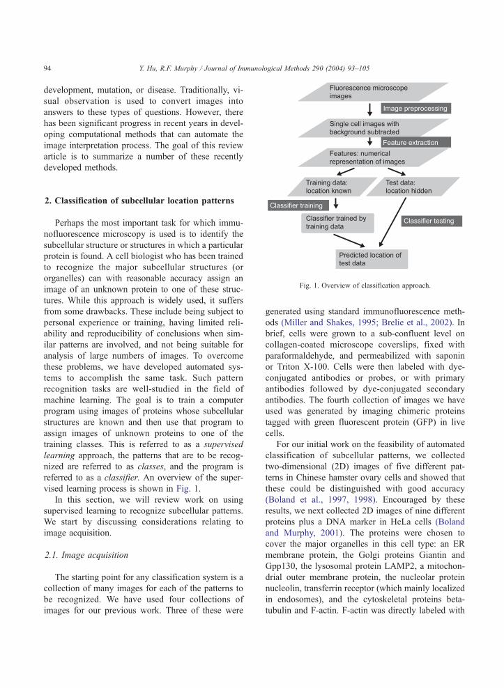
Fig. 1. Overview of classification approach.
2. Classification of subcellular location patterns
Perhaps the most important task for which immu-
nofluorescence microscopy is used is to identify the
subcellular structure or structures in which a particular
protein is found. A cell biologist who has been trained
to recognize the major subcellular structures (or
organelles) can with reasonable accuracy assign an
image of an unknown protein to one of these struc-
tures. While this approach is widely used, it suffers
from some drawbacks. These include being subject to
personal experience or training, having limited reli-
ability and reproducibility of conclusions when sim-
ilar patterns are involved, and not being suitable for
analysis of large numbers of images. To overcome
these problems, we have developed automated sys-
tems to accomplish the same task. Such pattern
recognition tasks are well-studied in the field of
machine learning. The goal is to train a computer
program using images of proteins whose subcellular
structures are known and then use that program to
assign images of unknown proteins to one of the
training classes. This is referred to as a supervised
learning approach, the patterns that are to be recog-
nized are referred to as classes, and the program is
referred to as a classifier. An overview of the super-
vised learning process is shown in Fig. 1.
In this section, we will review work on using
supervised learning to recognize subcellular patterns.
We start by discussing considerations relating to
image acquisition.
2.1. Image acquisition
The starting point for any classification system is a
collection of many images for each of the patterns to
be recognized. We have used four collections of
images for our previous work. Three of these were
generated using standard immunofluorescence meth-
ods (Miller and Shakes, 1995; Brelie et al., 2002). In
brief, cells were grown to a sub-confluent level on
collagen-coated microscope coverslips, fixed with
paraformaldehyde, and permeabilized with saponin
or Triton X-100. Cells were then labeled with dye-
conjugated antibodies or probes, or with primary
antibodies followed by dye-conjugated secondary
antibodies. The fourth collection of images we have
used was generated by imaging chimeric proteins
tagged with green fluorescent protein (GFP) in live
cells.
For our initial work on the feasibility of automated
classification of subcellular patterns, we collected
two-dimensional (2D) images of five different pat-
terns in Chinese hamster ovary cells and showed that
these could be distinguished with good accuracy
(Boland et al., 1997, 1998). Encouraged by these
results, we next collected 2D images of nine different
proteins plus a DNA marker in HeLa cells (Boland
and Murphy, 2001). The proteins were chosen to
cover the major organelles in this cell type: an ER
membrane protein, the Golgi proteins Giantin and
Gpp130, the lysosomal protein LAMP2, a mitochon-
drial outer membrane protein, the nucleolar protein
nucleolin, transferrin receptor (which mainly localized
in endosomes), and the cytoskeletal proteins beta-
tubulin and F-actin. F-actin was directly labeled with
Y. Hu, R.F. Murphy / Journal of Immunological Methods 290 (2004) 93–105 95
rhodamine phalloidin, nucleolin was labeled with
Cy3-conjugated antibodies and the other proteins
were labeled by Cy5-conjugated secondary antibod-
ies. All cells were incubated with DAPI to label DNA.
The 2D CHO and 2D HeLa collections were both
acquired using a wide-field fluorescence microscope
with nearest neighbor correction for out of focus
fluorescence.
To examine the potential value of collecting full
three-dimensional (3D) images rather than just 2D
slices, a collection of 3D images of HeLa cells was
also created (Velliste and Murphy, 2002). Images were
taken of the same nine proteins as in the 2D HeLa
collection using a three-laser confocal microscope.
Three probes were imaged for each sample: one for
the specific protein being labeled, one for total DNA,
and one for total protein. As discussed below, the
combination of the DNA and total protein images
permitted us to perform automated segmentation of
images into regions corresponding to single cells.
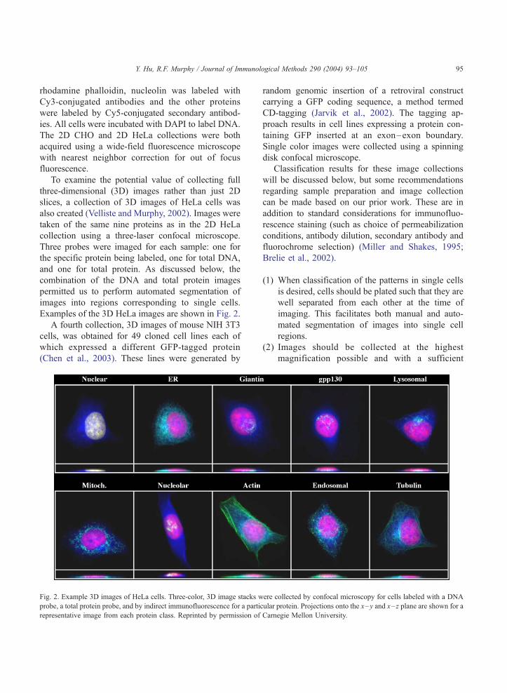
Examples of the 3D HeLa images are shown in Fig. 2.
A fourth collection, 3D images of mouse NIH 3T3
cells, was obtained for 49 cloned cell lines each of
which expressed a different GFP-tagged protein
(Chen et al., 2003). These lines were generated by
Fig. 2. Example 3D images of HeLa cells. Three-color, 3D image stacks w
probe, a total protein probe, and by indirect immunofluorescence for a partic
representative image from each protein class. Reprinted by permission of
random genomic insertion of a retroviral construct
carrying a GFP coding sequence, a method termed
CD-tagging (Jarvik et al., 2002). The tagging ap-
proach results in cell lines expressing a protein con-
taining GFP inserted at an exon–exon boundary.
Single color images were collected using a spinning
disk confocal microscope.
Classification results for these image collections
will be discussed below, but some recommendations
regarding sample preparation and image collection
can be made based on our prior work. These are in
addition to standard considerations for immunofluo-
rescence staining (such as choice of permeabilization
conditions, antibody dilution, secondary antibody and
fluorochrome selection) (Miller and Shakes, 1995;
Brelie et al., 2002).
(1) When classification of the patterns in single cells
is desired, cells should be plated such that they are
well separated from each other at the time of
imaging. This facilitates both manual and auto-
mated segmentation of images into single cell
regions.
(2) Images should be collected at the highest
magnification possible and with a sufficient
ere collected by confocal microscopy for cells labeled with a DNA
ular protein. Projections onto the x–y and x– z plane are shown for a
Carnegie Mellon University.
Y. Hu, R.F. Murphy / Journal of Immunological Methods 290 (2004) 93–10596
number of pixels so that optimal sampling of the
sample is achieved. The size of the pixels in the
plane of the sample can be calculated simply
using the magnification of the objective (and any
additional elements such as an optivar before the
camera) and the size of the pixels of the camera.
For example, a camera with 23-Am square pixels
used with a 100� objective collects light from
0.23-Am square regions in the sample plane. To
extract the maximum information from the
sample, images should be collected using pixels
small enough to achieve Nyquist sampling. The
Sampling Theorem states that an image must be
sampled at twice the highest frequency signal
actually present in the image (this is called the
Nyquist frequency). The Rayleigh criterion gives
the closest spacing between two objects that can
be resolved using a given microscope objective,
which is 1.22k/2NA. Thus, for 520-nm light being
emitted from fluorescein or GFP and a micro-
scope objective with a numerical aperture of 1.3,
the Rayleigh criterion is 244 nm. If this is the
highest frequency of meaningful information in
the image, then the maximum pixel size that
would achieve Nyquist sampling is 122 nm. The
image collections described above were acquired
using a 60� (3D 3T3) or 100� (others) objective
and with a pixel size from 0.049 to 0.23 Am,
which means that they were near or at Nyquist
sampling.
(3) Images should be collected with at least one cell
entirely within the field. In many cases, accurate
classification or comparison of patterns depends
on the assumption that a whole cell is being
imaged. For example, the number of fluorescent
objects per cell or the average distance between
objects and the center of fluorescence are both
features frequently used for automated analysis
that require a full cell image.
(4) The number of images acquired for each condition
should be sufficient to enable statistically signif-
icant comparisons. This can be as few as a single
cell image if the goal is to use a classifier trained
on large numbers of cells previously acquired
under identical conditions, but more commonly
consists of at least as many cell images as the
number of features that will be used to analyze
them (see below for discussion of feature sets).
This usually consists of at least 50 cells per
condition, and this is a very feasible number given
current digital microscopes and the low cost and
high capacity of storage media.
(5) Images should be acquired using microscope
settings as close to identical as possible for all
conditions. While it may be possible to normalize
features to compensate for differences in settings,
in most cases changing factors such as camera
gain, z-slice spacing or integration time between
conditions dramatically limits the confidence with
which comparisons or classifications can be
made.
(6) If possible, parallel images of total DNA and total
protein content should be acquired. While not
necessary for recognition of most patterns,
availability of a parallel DNA image allows
additional features to be calculated and improves
classification accuracy. If a total protein image is
also available, automated segmentation of images
into single cell regions can be performed,
eliminating the need for performing this step
manually. An alternative to a parallel total protein
image is a parallel image of a protein that is
predominantly located in the plasma membrane.
The latter approach has been used to segment
tissue images into single cell regions (De Solo-
rzano et al., 2001).
(7) It is critical that images to be used for automated
analysis be appropriately organized and annotat-
ed. The preferred method is annotation within
each file at the time of acquisition, but grouping
and annotation after collection are acceptable as
long as care is taken to ensure the accuracy of any
post-acquisition annotations.
2.2. Image preprocessing and segmentation
The goal of these steps is to prepare single cell
images that are suitable for extraction of numerical
features.
Deconvolution: For our image collections acquired
with a wide-field microscope, a minimum of three
closely spaced optical sections were collected and
numerical deconvolution was used to reduce out of
focus fluorescence. While we recommend using either
confocal images or numerically deconvolved images,
it should be noted that we have not determined
Y. Hu, R.F. Murphy / Journal of Immunological Methods 290 (2004) 93–105 97
whether deconvolution is required to achieve satisfac-
tory classification results.
Background subtraction/correction: So that fea-
tures reflecting fluorescence intensity are accurate,
some approach should be used to correct for back-
ground fluorescence. We have used the simple ap-
proach of subtracting the most common pixel value
(based on the assumption that an image contains more
pixels outside the cell than inside it and that back-
ground is roughly uniform). Alternatives include sub-
tracting an image of a blank field or making estimates
of the background in local regions.
Cropping/segmentation: Cropping or segmentation
refers to identifying regions within an image that
contain only a single cell. These can be generated
by drawing polygons on an image that surround
individual cells, or by automated methods. Once the
region is identified, pixels outside the region are set to
zero. More than one region can be identified in each
image.
Thresholding: The morphological features de-
scribed below require identification of fluorescent
objects within a cell. Our current approach defines
objects as connected pixels that are ‘‘positive’’ for
fluorescence, i.e., that are above a threshold. This
threshold is chosen by an automated method (Ridler
and Calvard, 1978), and pixels below the threshold
are set to zero. For simplicity, we use the thresholded
image to calculate all features, although thresholding
is not required for calculating texture or moment
features.
Normalization: The goal of our subcellular pattern
analysis is to compare protein patterns without con-
sidering protein abundance. Each pixel (or voxel)
value is therefore divided by the total fluorescence
in the image.
2.3. Subcellular location features
For images, two kinds of inputs to a classifier can
be used: the intensity values of the pixels (or voxels) in
the images themselves, or the values of features
derived from the images. (It is worth nothing that
while the ‘‘inputs’’ to visual classification are always
the pixel values, it is unclear whether biologists trying
to classify such images operate on the image directly
or use features they derive from visual processing of
the image.) Eukaryotic cells differ dramatically in size
and shape, even within a single cell type. We have
therefore avoided pattern recognition methods that
operate directly on images and have instead used
methods that begin by extracting numerical features
to describe elements of the patterns in cell images.
This process is illustrated in Fig. 3. The features we
have used are invariant to translation, rotation and
total intensity of fluorescence, and are robust to
differences in cell shape, cell types, and fluorescence
microscopy methods. Many such features can be
imagined and we incorporate new features or modify
old ones on an ongoing basis.
To facilitate identification of the features used for a
particular experiment or system, we have defined
conventions for referring to features used to classify
subcellular patterns. We refer to sets of these as SLF
(for Subcellular Location Features) followed by a
number (e.g., SLF7) and to individual features by
the set number followed by the index within that set
(e.g., SLF1.3 refers to the 3rd feature in set 1). A
summary of the currently defined SLF is presented in
Tables 1 and 2.
The SLF are of nine basic types. Each type is
briefly described below.
Morphological (SLF1.1–1.8 and SLF7.79): In
general, morphological features describe how intensi-
ty (in this case fluorescence) is grouped. We have
described specific morphological features that are
valuable for analyzing protein patterns (Boland and
Murphy, 2001; Murphy et al., 2002). Contiguous
groups of non-zero pixels in a thresholded image are
defined as objects and contiguous group of zero-
valued pixels surrounded by non-zero pixels as holes.
Various features can be calculated from the set of
identified objects, including number of objects per
cell, number of objects minus number of holes per
cell, average number of pixels per object, average
distance of objects to the center of fluorescence (COF)
and the fraction of fluorescence not included in
objects.
Edge (SLF7.9–7.13): The set of edges in an image
can be found using one of various filtering methods.
Edge features that can be calculated from the set of
edges include the fraction of pixels distributed along
edges, and measures of how homogeneous edges are
in intensity and direction (Boland and Murphy, 2001).
Geometric (SLF1.14–1.16): These features are
derived from the convex hull of the image, which is
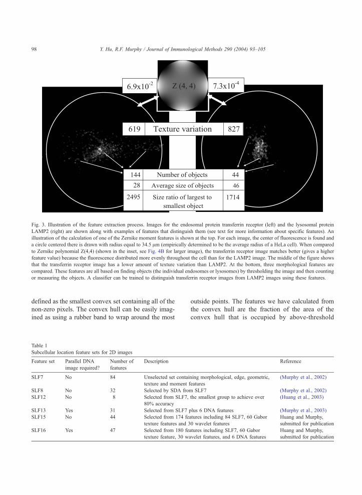
Fig. 3. Illustration of the feature extraction process. Images for the endosomal protein transferrin receptor (left) and the lysosomal protein
LAMP2 (right) are shown along with examples of features that distinguish them (see text for more information about specific features). An
illustration of the calculation of one of the Zernike moment features is shown at the top. For each image, the center of fluorescence is found and
a circle centered there is drawn with radius equal to 34.5 Am (empirically determined to be the average radius of a HeLa cell). When compared
to Zernike polynomial Z(4,4) (shown in the inset, see Fig. 4B for larger image), the transferrin receptor image matches better (gives a higher
feature value) because the fluorescence distributed more evenly throughout the cell than for the LAMP2 image. The middle of the figure shows
that the transferrin receptor image has a lower amount of texture variation than LAMP2. At the bottom, three morphological features are
compared. These features are all based on finding objects (the individual endosomes or lysosomes) by thresholding the image and then counting
or measuring the objects. A classifier can be trained to distinguish transferrin receptor images from LAMP2 images using these features.
Y. Hu, R.F. Murphy / Journal of Immunological Methods 290 (2004) 93–10598
defined as the smallest convex set containing all of the
non-zero pixels. The convex hull can be easily imag-
ined as using a rubber band to wrap around the most
Table 1
Subcellular location feature sets for 2D images
Feature set Parallel DNA
image required?
Number of
features
Description
SLF7 No 84 Unselected set contai
texture and moment
SLF8 No 32 Selected by SDA fro
SLF12 No 8 Selected from SLF7,
80% accuracy
SLF13 Yes 31 Selected from SLF7
SLF15 No 44 Selected from 174 fe
texture features and 3
SLF16 Yes 47 Selected from 180 fe
texture feature, 30 w
outside points. The features we have calculated from
the convex hull are the fraction of the area of the
convex hull that is occupied by above-threshold
Reference
ning morphological, edge, geometric,
features
(Murphy et al., 2002)
m SLF7 (Murphy et al., 2002)
the smallest group to achieve over (Huang et al., 2003)
plus 6 DNA features (Murphy et al., 2003)
atures including 84 SLF7, 60 Gabor
0 wavelet features
Huang and Murphy,
submitted for publication
atures including SLF7, 60 Gabor
avelet features, and 6 DNA features
Huang and Murphy,
submitted for publication
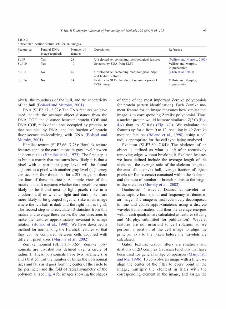
Table 2
Subcellular location feature sets for 3D images
Feature set Parallel DNA
image required?
Number of
features
Description Reference
SLF9 Yes 28 Unselected set containing morphological features (Velliste and Murphy, 2002)
SLF10 Yes 9 Selected by SDA from SLF9 Velliste and Murphy,
in preparation
SLF11 No 42 Unselected set containing morphological, edge
and texture features
(Chen et al., 2003)
SLF14 No 14 Features in SLF9 that do not require a parallel
DNA image
Velliste and Murphy,
in preparation
Y. Hu, R.F. Murphy / Journal of Immunological Methods 290 (2004) 93–105 99
pixels, the roundness of the hull, and the eccentricity
of the hull (Boland and Murphy, 2001).
DNA (SLF2.17–2.22): The DNA features we have
used include the average object distance from the
DNA COF, the distance between protein COF and
DNA COF, ratio of the area occupied by proteins to
that occupied by DNA, and the fraction of protein
fluorescence co-localizing with DNA (Boland and
Murphy, 2001).
Haralick texture (SLF7.66–7.78): Haralick texture
features capture the correlations in gray level between
adjacent pixels (Haralick et al., 1973). The first step is
to build a matrix that measures how likely it is that a
pixel with a particular gray level will be found
adjacent to a pixel with another gray level (adjacency
can occur in four directions for a 2D image, so there
are four of these matrices). A simple view of this
matrix is that it captures whether dark pixels are more
likely to be found next to light pixels (like in a
checkerboard) or whether light and dark pixels are
more likely to be grouped together (like in an image
where the left half is dark and the right half is light).
The second step is to calculate 13 statistics from this
matrix and average these across the four directions to
make the features approximately invariant to image
rotation (Boland et al., 1998). We have described a
method for normalizing the Haralick features so that
they can be compared between cells acquired with
different pixel sizes (Murphy et al., 2002).
Zernike moment (SLF3.17–3.65): Zernike poly-
nomials are distributions defined over a circle of
radius 1. These polynomials have two parameters, n
and l that control the number of times the polynomial
rises and falls as it goes from the center of the circle to
the perimeter and the fold of radial symmetry of the
polynomial (see Fig. 4 for images showing the shapes
of three of the most important Zernike polynomials
for protein pattern identification). Each Zernike mo-
ment feature for an image measures how similar that
image is to corresponding Zernike polynomial. Thus,
a nuclear protein would be more similar to Z(2,0) (Fig.
4A) than to Z(10,6) (Fig. 4C). We calculate the
features up for n from 0 to 12, resulting in 49 Zernike
moment features (Boland et al., 1998), using a cell
radius appropriate for the cell type being analyzed.
Skeleton (SLF7.80–7.84): The skeleton of an
object is defined as what is left after recursively
removing edges without breaking it. Skeleton features
we have defined include the average length of the
skeletons, the average ratio of the skeleton length to
the area of its convex hull, average fraction of object
pixels (or fluorescence) contained within the skeleton,
and the ratio of number of branch points to the length
in the skeleton (Murphy et al., 2002).
Daubechies 4 wavelet: Daubechies wavelet fea-
tures capture both spatial and frequency attributes of
an image. The image is first recursively decomposed
to fine and coarse approximations using a discrete
wavelet transformation and then the average energies
within each quadrant are calculated as features (Huang
and Murphy, submitted for publication). Wavelet
features are not invariant to cell rotation, so we
perform a rotation of the cell image to align the
principal axis to the y-axis before the wavelets are
calculated.
Gabor texture: Gabor filters are rotations and
dilations of 2D complex Gaussian functions that have
been used for general image comparison (Manjunath
and Ma, 1996). To convolve an image with a filter, we
align the center of the filter to every point in the
image, multiply the element in filter with the
corresponding element in the image, and assign the
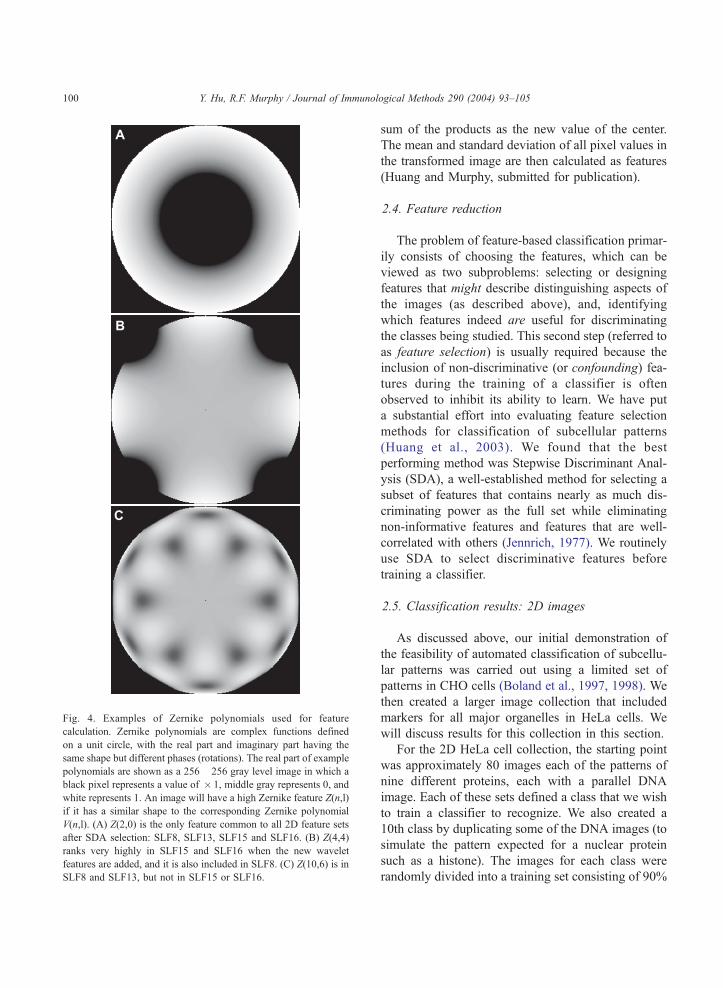
Fig. 4. Examples of Zernike polynomials used for feature
calculation. Zernike polynomials are complex functions defined
on a unit circle, with the real part and imaginary part having the
same shape but different phases (rotations). The real part of example
polynomials are shown as a 256� 256 gray level image in which a
black pixel represents a value of � 1, middle gray represents 0, and
white represents 1. An image will have a high Zernike feature Z(n,l)
if it has a similar shape to the corresponding Zernike polynomial
V(n,l). (A) Z(2,0) is the only feature common to all 2D feature sets
after SDA selection: SLF8, SLF13, SLF15 and SLF16. (B) Z(4,4)
ranks very highly in SLF15 and SLF16 when the new wavelet
features are added, and it is also included in SLF8. (C) Z(10,6) is in
SLF8 and SLF13, but not in SLF15 or SLF16.
Y. Hu, R.F. Murphy / Journal of Immunological Methods 290 (2004) 93–105100
sum of the products as the new value of the center.
The mean and standard deviation of all pixel values in
the transformed image are then calculated as features
(Huang and Murphy, submitted for publication).
2.4. Feature reduction
The problem of feature-based classification primar-
ily consists of choosing the features, which can be
viewed as two subproblems: selecting or designing
features that might describe distinguishing aspects of
the images (as described above), and, identifying
which features indeed are useful for discriminating
the classes being studied. This second step (referred to
as feature selection) is usually required because the
inclusion of non-discriminative (or confounding) fea-
tures during the training of a classifier is often
observed to inhibit its ability to learn. We have put
a substantial effort into evaluating feature selection
methods for classification of subcellular patterns
(Huang et al., 2003). We found that the best
performing method was Stepwise Discriminant Anal-
ysis (SDA), a well-established method for selecting a
subset of features that contains nearly as much dis-
criminating power as the full set while eliminating
non-informative features and features that are well-
correlated with others (Jennrich, 1977). We routinely
use SDA to select discriminative features before
training a classifier.
2.5. Classification results: 2D images
As discussed above, our initial demonstration of
the feasibility of automated classification of subcellu-
lar patterns was carried out using a limited set of
patterns in CHO cells (Boland et al., 1997, 1998). We
then created a larger image collection that included
markers for all major organelles in HeLa cells. We
will discuss results for this collection in this section.
For the 2D HeLa cell collection, the starting point
was approximately 80 images each of the patterns of
nine different proteins, each with a parallel DNA
image. Each of these sets defined a class that we wish
to train a classifier to recognize. We also created a
10th class by duplicating some of the DNA images (to
simulate the pattern expected for a nuclear protein
such as a histone). The images for each class were
randomly divided into a training set consisting of 90%
Y. Hu, R.F. Murphy / Journal of Immunological Methods 290 (2004) 93–105 101
of the images and a test set consisting of the remaining
10%. The features for the training set were used to
adjust the parameters of a classifier until that classifier
was able to recognize those training images as accu-
rately as possible. The training was stopped, the
features for the test images were supplied to the
classifier, and the class predicted by the classifier
was recorded for each image. The results can be
tabulated in a confusion matrix in which each row
represents the known class of a particular image and
the columns represent the predicted class. Each ele-
ment in a confusion matrix is the percentage of images
of the known class of that row that were predicted as
the being the class of that column. The elements on
the diagonal are therefore the percentages of correct
predictions and the overall accuracy of a confusion
matrix is the average of these diagonal values.
We defined feature set SLF3 as a combination of
morphological, edge, geometric, Haralick texture, and
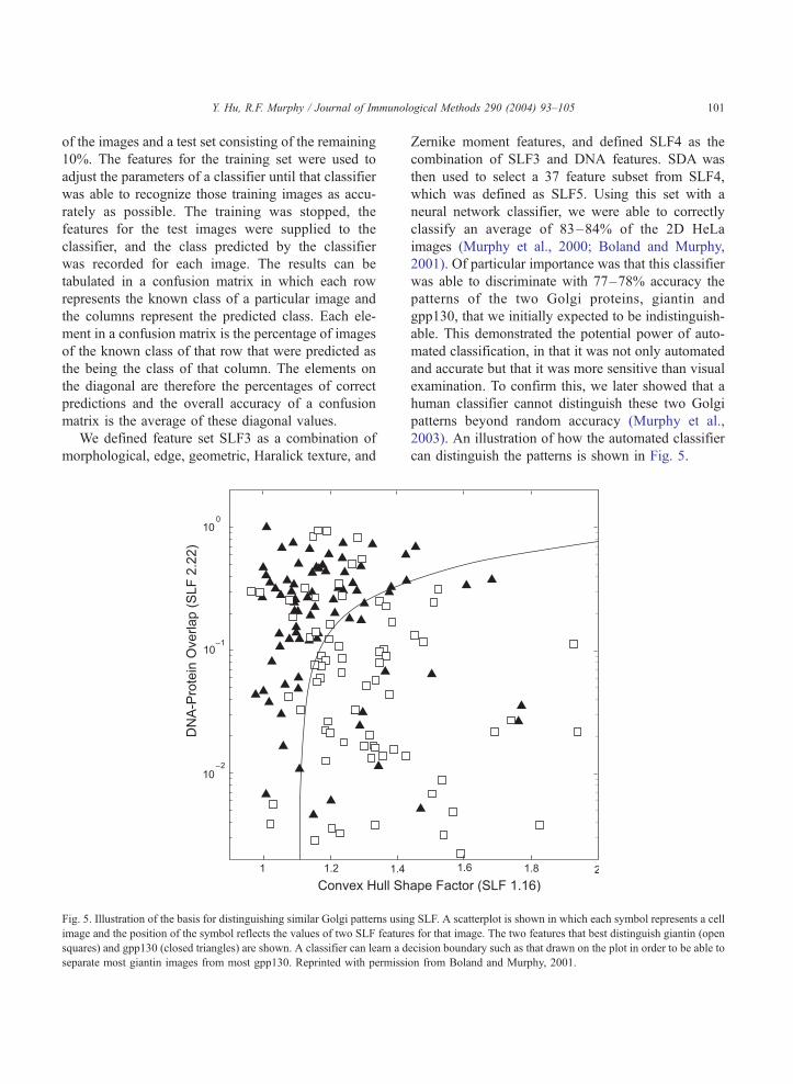
Fig. 5. Illustration of the basis for distinguishing similar Golgi patterns usin
image and the position of the symbol reflects the values of two SLF feature
squares) and gpp130 (closed triangles) are shown. A classifier can learn a d
separate most giantin images from most gpp130. Reprinted with permissi
Zernike moment features, and defined SLF4 as the
combination of SLF3 and DNA features. SDA was
then used to select a 37 feature subset from SLF4,
which was defined as SLF5. Using this set with a
neural network classifier, we were able to correctly
classify an average of 83–84% of the 2D HeLa
images (Murphy et al., 2000; Boland and Murphy,
2001). Of particular importance was that this classifier
was able to discriminate with 77–78% accuracy the
patterns of the two Golgi proteins, giantin and
gpp130, that we initially expected to be indistinguish-
able. This demonstrated the potential power of auto-
mated classification, in that it was not only automated
and accurate but that it was more sensitive than visual
examination. To confirm this, we later showed that a
human classifier cannot distinguish these two Golgi
patterns beyond random accuracy (Murphy et al.,
2003). An illustration of how the automated classifier
can distinguish the patterns is shown in Fig. 5.
g SLF. A scatterplot is shown in which each symbol represents a cell
s for that image. The two features that best distinguish giantin (open
ecision boundary such as that drawn on the plot in order to be able to
on from Boland and Murphy, 2001.
Y. Hu, R.F. Murphy / Journal of Immunological Methods 290 (2004) 93–105102
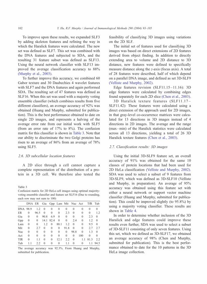
To improve upon these results, we expanded SLF3
by adding skeleton features and refining the way in
which the Haralick features were calculated. The new
set was defined as SLF7. This set was combined with
the DNA features and subjected to SDA, and the
resulting 31 feature subset was defined as SLF13.
Using the neural network classifier with SLF13 im-
proved the average classification accuracy to 88%
(Murphy et al., 2003).
To further improve this accuracy, we combined 60
Gabor texture and 30 Daubechies 4 wavelet features
with SLF7 and the DNA features and again performed
SDA. The resulting set of 47 features was defined as
SLF16. When this set was used with a majority voting
ensemble classifier (which combines results from five
different classifiers), an average accuracy of 92% was
obtained (Huang and Murphy, submitted for publica-
tion). This is the best performance obtained to date on
single 2D images, and represents a halving of the
average error rate from our initial work with SLF5
(from an error rate of 17% to 8%). The confusion
matrix for this classifier is shown in Table 3. Note that
our ability to discriminate the two Golgi proteins has
risen to an average of 86% from an average of 78%
using SLF5.
2.6. 3D subcellular location features
A 2D slice through a cell cannot capture a
complete representation of the distribution of a pro-
tein in a 3D cell. We therefore also tested the
Table 3
Confusion matrix for 2D HeLa cell images using optimal majority-
voting ensemble classifier and feature set SLF16 (Due to rounding,
each row may not sum to 100)
DNA ER Gia Gpp Lam Mit Nuc Act TfR Tub
DNA 98.9 1.2 0 0 0 0 0 0 0 0
ER 0 96.5 0 0 0 2.3 0 0 0 1.2
Gia 0 0 90.8 6.9 0 0 0 0 2.3 0
Gpp 0 0 14.1 82.4 0 0 2.4 0 1.2 0
Lam 0 0 1.2 0 88.1 1.2 0 0 9.5 0
Mit 0 2.7 0 0 0 91.8 0 0 2.7 2.7
Nuc 0 0 0 0 0 0 98.8 0 1.3 0
Act 0 0 0 0 0 0 0 100 0 0
TfR 0 1.1 0 0 12.1 2.2 0 1.1 81.3 2.2
Tub 1.1 2.2 0 0 0 1.1 0 0 1.1 94.5
The average accuracy was 92.3%. From Huang and Murphy,
submitted for publication.
feasibility of classifying 3D images using variations
on the 2D SLF.
The initial set of features used for classifying 3D
images was based on direct extensions of 2D features
derived from object finding. In addition to directly
extending area to volume and 2D distance to 3D
distance, new features were defined to specifically
measure distance along the z-axis (focus axis). A total
of 28 features were described, half of which depend
on a parallel DNA image, and defined as set 3D-SLF9
(Velliste and Murphy, 2002).
Edge features revision (SLF11.15–11.16): 3D
edge features were calculated by combining edges
found separately for each 2D slice (Chen et al., 2003).
3D Haralick texture features (SLF11.17 –
SLF11.42): These features were calculated using a
direct extension of the approach used for 2D images,
in that gray-level co-occurrence matrices were calcu-
lated for 13 directions in 3D images instead of 4
directions in 2D images. The average and the range
(max–min) of the Haralick statistics were calculated
across all 13 directions, yielding a total of 26 3D
Haralick texture features (Chen et al., 2003).
2.7. Classification results: 3D images
Using the initial 3D-SLF9 feature set, an overall
accuracy of 91% was obtained for the same 10
classes of protein locations that had been used for
2D HeLa classification (Velliste and Murphy, 2002).
SDA was used to select a subset of 9 features from
3D-SLF9, which was defined as 3D-SLF10 (Velliste
and Murphy, in preparation). An average of 95%
accuracy was obtained using this feature set with
either a neural network or support vector machine
classifier (Huang and Murphy, submitted for publica-
tion). This could be improved slightly (to 95.8%) by
using a majority voting classifier. These results are
shown in Table 4.
In order to determine whether inclusion of the 3D
Haralick and edge features could improve these
results even further, SDA was used to select a subset
of 3D-SLF11 consisting of only seven features. Using
this set, which we defined as 3D-SLF17, we obtained
an average accuracy of 98% (Chen and Murphy,
submitted for publication). This is the best perfor-
mance obtained to date for the 10 patterns in the 3D
HeLa image collection.
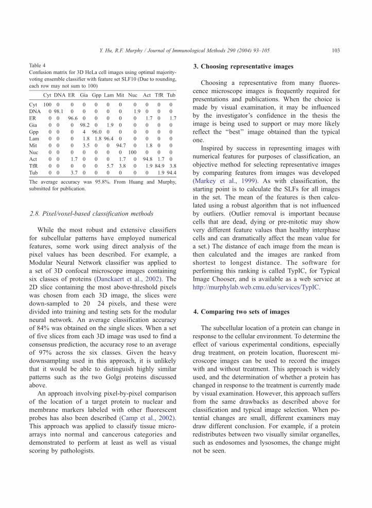
Table 4
Confusion matrix for 3D HeLa cell images using optimal majority-
voting ensemble classifier with feature set SLF10 (Due to rounding,
each row may not sum to 100)
Cyt DNA ER Gia Gpp Lam Mit Nuc Act TfR Tub
Cyt 100 0 0 0 0 0 0 0 0 0 0
DNA 0 98.1 0 0 0 0 0 1.9 0 0 0
ER 0 0 96.6 0 0 0 0 0 1.7 0 1.7
Gia 0 0 0 98.2 0 1.9 0 0 0 0 0
Gpp 0 0 0 4 96.0 0 0 0 0 0 0
Lam 0 0 0 1.8 1.8 96.4 0 0 0 0 0
Mit 0 0 0 3.5 0 0 94.7 0 1.8 0 0
Nuc 0 0 0 0 0 0 0 100 0 0 0
Act 0 0 1.7 0 0 0 1.7 0 94.8 1.7 0
TfR 0 0 0 0 0 5.7 3.8 0 1.9 84.9 3.8
Tub 0 0 3.7 0 0 0 0 0 0 1.9 94.4
The average accuracy was 95.8%. From Huang and Murphy,
submitted for publication.
Y. Hu, R.F. Murphy / Journal of Immunological Methods 290 (2004) 93–105 103
2.8. Pixel/voxel-based classification methods
While the most robust and extensive classifiers
for subcellular patterns have employed numerical
features, some work using direct analysis of the
pixel values has been described. For example, a
Modular Neural Network classifier was applied to
a set of 3D confocal microscope images containing
six classes of proteins (Danckaert et al., 2002). The
2D slice containing the most above-threshold pixels
was chosen from each 3D image, the slices were
down-sampled to 20� 24 pixels, and these were
divided into training and testing sets for the modular
neural network. An average classification accuracy
of 84% was obtained on the single slices. When a set
of five slices from each 3D image was used to find a
consensus prediction, the accuracy rose to an average
of 97% across the six classes. Given the heavy
downsampling used in this approach, it is unlikely
that it would be able to distinguish highly similar
patterns such as the two Golgi proteins discussed
above.
An approach involving pixel-by-pixel comparison
of the location of a target protein to nuclear and
membrane markers labeled with other fluorescent
probes has also been described (Camp et al., 2002).
This approach was applied to classify tissue micro-
arrays into normal and cancerous categories and
demonstrated to perform at least as well as visual
scoring by pathologists.
3. Choosing representative images
Choosing a representative from many fluores-
cence microscope images is frequently required for
presentations and publications. When the choice is
made by visual examination, it may be influenced
by the investigator’s confidence in the thesis the
image is being used to support or may more likely
reflect the ‘‘best’’ image obtained than the typical
one.
Inspired by success in representing images with
numerical features for purposes of classification, an
objective method for selecting representative images
by comparing features from images was developed
(Markey et al., 1999). As with classification, the
starting point is to calculate the SLFs for all images
in the set. The mean of the features is then calcu-
lated using a robust algorithm that is not influenced
by outliers. (Outlier removal is important because
cells that are dead, dying or pre-mitotic may show
very different feature values than healthy interphase
cells and can dramatically affect the mean value for
a set.) The distance of each image from the mean is
then calculated and the images are ranked from
shortest to longest distance. The software for
performing this ranking is called TypIC, for Typical
Image Chooser, and is available as a web service at
http://murphylab.web.cmu.edu/services/TypIC.
4. Comparing two sets of images
The subcellular location of a protein can change in
response to the cellular environment. To determine the
effect of various experimental conditions, especially
drug treatment, on protein location, fluorescent mi-
croscope images can be used to record the images
with and without treatment. This approach is widely
used, and the determination of whether a protein has
changed in response to the treatment is currently made
by visual examination. However, this approach suffers
from the same drawbacks as described above for
classification and typical image selection. When po-
tential changes are small, different examiners may
draw different conclusion. For example, if a protein
redistributes between two visually similar organelles,
such as endosomes and lysosomes, the change might
not be seen.
Y. Hu, R.F. Murphy / Journal of Immunological Methods 290 (2004) 93–105104
An alternative is to use pattern analysis methods to
compare sets of images (Roques and Murphy, 2002).
Again, the SLFs can be used to represent images, and
the comparison becomes determining whether the
features of the two sets of images are statistically
different. Each set of images is represented by an n*m
matrix, where n is the number of images and m is the
number of features. Every row contains a feature
vector extracted from one image. The Statistical
Imaging Experiment Comparator (SImEC) system
(Roques and Murphy, 2002) compares the feature
matrices for the two sets using the multivariate ver-
sion of the traditional t-test, the Hotelling T 2-test. The
result is an F statistic with 2 degrees of freedom: the
number of features, and the total number of images
minus the number of features. If the F value is larger
than a critical value determined for those degrees of
freedom and a particular confidence level, then the
two sets can be considered to be different at that
confidence level.
When this approach was used to perform pairwise
comparisons on the 10 classes of the 2D HeLa image
collection, all 10 classes were found to be statistically
distinguishable at the 95% confidence level. This is
consistent with our ability to train classifiers to
distinguish them with high accuracy. In control
experiments, the SImEC system obtained the correct
results when two subsets drawn from the same image
class were compared. An additional control experi-
ment was performed in which two different probes
were used to label the same protein, giantin. Sets of
images obtained by indirect immunofluorescence us-
ing either a rabbit anti-giantin antiserum or a mouse
anti-giantin monoclonal antibody were found to be
statistically indistinguishable at the 95% confidence
level. This result confirms that the SImEC approach
can appropriately distinguish patterns that are differ-
ent while still considering as indistinguishable pat-
terns that should be the same.
5. Implications for cell and molecular biology
research
The combination of readily available digital fluo-
rescence microscopes with the methods described
here has the potential for significantly changing the
way in which immunofluorescence microscopy is
used to answer biological questions. Whether for
high-throughput determination of the major subcellu-
lar organelle in which unknown proteins are found or
for determining whether a protein changes its distri-
bution in response to a particular drug or transgene,
computerized methods have been shown to be signif-
icantly easier to use, more accurate, and more sensi-
tive than visual examination. The availability of these
methods can be expected to add an important quan-
titative and objective element to cell biology experi-
ments that will facilitate their use both in detailed
characterization of individual proteins and in large-
scale proteomics efforts.
Acknowledgements
We thank Kai Huang for helpful discussions. The
original research described in this chapter was
supported in part by research grant RPG-95-099-03-
MGO from the American Cancer Society, by NSF
grants BIR-9217091, MCB-8920118, and BIR-
9256343, by NIH grants R01 GM068845 and R33
CA83219, and by a research grant from the
Commonwealth of Pennsylvania Tobacco Settlement
Fund.
References
Boland, M.V., Murphy, R.F., 2001. A neural network classifier
capable of recognizing the patterns of all major subcellular
structures in fluorescence microscope images of HeLa cells.
Bioinformatics 17, 1213.
Boland, M.V., Markey, M.K., Murphy, R.F., 1997. Classification of
protein localization patterns obtained via fluorescence light mi-
croscopy. 19th Annual International Conference of the IEEE
Engineering in Medicine and Biology Society, Chicago, IL,
USA. IEEE, p. 594.
Boland, M.V., Markey, M.K., Murphy, R.F., 1998. Automated rec-
ognition of patterns characteristic of subcellular structures in
fluorescence microscopy images. Cytometry 33, 366.
Brelie, T.C., Wessendorf, M.W., Sorenson, R.L., 2002. Multicolor
laser scanning confocal immunofluorescence microscopy: prac-
tical application and limitations. Methods Cell Biol. 70, 165.
Camp, R.L., Chung, G.G., Rimm, D.L., 2002. Automated subcel-
lular localization and quantification of protein expression in
tissue microarrays. Nat. Med. 8, 1323.
Chen, X., Velliste, M., Weinstein, S., Jarvik, J.W., Murphy, R.F.,
2003. Location proteomics—building subcellular location trees
from high resolution 3D fluorescence microscope images of
randomly-tagged proteins. Proc. SPIE 4962, 298.
Y. Hu, R.F. Murphy / Journal of Immunological Methods 290 (2004) 93–105 105
Danckaert, A., Gonzalez-Couto, E., Bollondi, L., Thompson, N.,
Hayes, B., 2002. Automated recognition of intracellular organ-
elles in confocal microscope images. Traffic 3, 66.
De Solorzano, C.O., Malladi, R., Lelievre, S.A., Lockett, S.J., 2001.
Segmentation of nuclei and cells using membrane related pro-
tein markers. J. Microsc. 201, 404.
Haralick, R., Shanmugam, K., Dinstein, I., 1973. Textural features
for image classification. IEEE Trans. Syst. Man Cybern. SMC-
3, 610.
Huang, K., Velliste, M., Murphy, R.F., 2003. Feature reduction for
improved recognition of subcellular location patterns in fluores-
cence microscope images. Proc. SPIE 4962, 307.
Jarvik, J.W., Fisher, G.W., Shi, C., Hennen, L., Hauser, C.,
Adler, S., Berget, P.B., 2002. In vivo functional proteomics:
mammalian genome annotation using CD-tagging. BioTechni-
ques 33, 852.
Jennrich, R.I., 1977. Stepwise discriminant analysis. In: Enslein, K.,
Ralston, A., Wilf, H.S. (Eds.), Statistical Methods for Digital
Computers, vol. 3. Wiley, New York, p. 77.
Manjunath, B.S., Ma, W.Y., 1996. Texture features for browsing
and retrieval of image data. IEEE Trans. Pattern Anal. Mach.
Intell. 8, 837.
Markey, M.K., Boland, M.V., Murphy, R.F., 1999. Towards objec-
tive selection of representative microscope images. Biophys. J.
76, 2230.
Miller, D.M., Shakes, D.C., 1995. Immunofluorescence microscopy.
Methods Cell Biol. 48, 365.
Murphy, R.F., Boland, M.V., Velliste, M., 2000. Towards a system-
atics for protein subcellular location: quantitative description of
protein localization patterns and automated analysis of fluores-
cence microscope images. Proc. Int. Conf. Intell. Syst. Mol.
Biol. 8, 251.
Murphy, R.F., Velliste, M., Porreca, G., 2002. Robust classification
of subcellular location patterns in fluorescence microscope
images. 2002 IEEE International Workshop on Neural Networks
for Signal Processing (NNSP 12). IEEE, p. 67.
Murphy, R.F., Velliste, M., Porreca, G., 2003. Robust numerical
features for description and classification of subcellular location
patterns in fluorescence microscope images. J. VLSI Signal
Process. 35, 311.
Ridler, T.W., Calvard, S., 1978. Picture thresholding using an iter-
ative selection method. IEEE Trans. Syst. Man Cybern. SMC-8,
630.
Roques, E.J.S., Murphy, R.F., 2002. Objective evaluation of differ-
ences in protein subcellular distribution. Traffic 3, 61.
Velliste, M., Murphy, R.F., 2002. Automated determination of pro-
tein subcellular locations from 3D fluorescence microscope
images. 2002 IEEE International Symposium on Biomedical
Imaging (ISBI-2002), Bethesda, MD, USA. IEEE, p. 867.
Recommended