PyECLOUDG. Iadarola, G. Rumolo
ECLOUD meeting 28/11/2011
Thanks to:R. De Maria, K. Li
Outline
• Why a new code for electron cloud build-up simulation?
• From ECLOUD to PyECLOUD
o Management of macroparticle size and number
o Back-tracking algorithm for the impacting electrons
o Beam field calculation
o Space charge field
• Preliminary convergence study
• PyECLOUD at work
• Conclusion and future work
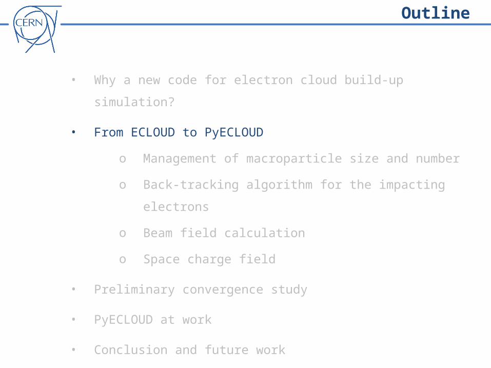
Why a new code for electron cloud build-up simulation?
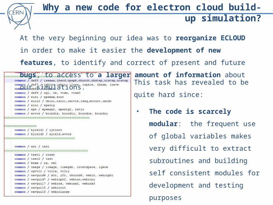
At the very beginning our idea was to reorganize ECLOUD in order to make it
easier the development of new features, to identify and correct of present and
future bugs, to access to a larger amount of information about our simulations.
Why a new code for electron cloud build-up simulation?
This task has revealed to be quite hard since:
• The code is scarcely modular: the
frequent use of global variables makes
very difficult to extract subroutines and
building self consistent modules for
development and testing purposes
• In Fortran 77 is very difficult to write
readable and flexible code (even a proper
indentation is a non-trivial task)
At the very beginning our idea was to reorganize ECLOUD in order to make it
easier the development of new features, to identify and correct of present and
future bugs, to access to a larger amount of information about our simulations.
Why a new code for electron cloud build-up simulation?
At the very beginning our idea was to reorganize ECLOUD in order to make it
easier the development of new features, to identify and correct of present and
future bugs, to access to a larger amount of information about our simulations.
We have retained that the effort of writing a fully reorganized code, in a newer
and more powerful language, should be compensated by a significantly increased
efficiency in future development and debugging.
Python
• Allows incremental and interactive development of the code, encouraging an
highly modular structure. Reading and understanding the code, writing
extensions, exploring different solutions is much faster (orders of magnitude!!)
with respect to compiled languages (especially looking at FORTRAN 77)
• Open source libraries (like NumPy and SciPy) make it a very powerful tool for
scientific computation (comparable to a specialized commercial tool like MATLAB)
• Computationally intensive parts can be written in C/C++ or FORTRAN and easily
integrated in a Python code (successfully employed in our distribution
computation/interpolation routines – x6 overall speed up)
It is a powerful general purpose interpreted language:
Outline
• Why a new code for electron cloud build-up simulation?
• From ECLOUD to PyECLOUD
o Management of macroparticle size and number
o Back-tracking algorithm for the impacting electrons
o Beam field calculation
o Space charge field
• Preliminary convergence study
• PyECLOUD at work
• Conclusion and future work
From ECLOUD to PyECLOUD
Writing PyECLOUD has required a detailed analysis of ECLOUD algorithm and
implementation, looking also at the related long experience in electron cloud simulations.
Attention has been devoted to the individuation of ECLOUD limitations, in particular in
terms of its convergence properties with respect to the electron distribution in bending
magnets (how many stripes…)
As a result, several features have been significantly modified in order to improve the
code’s performances in terms:
• Accuracy
• Efficiency
• Flexibility
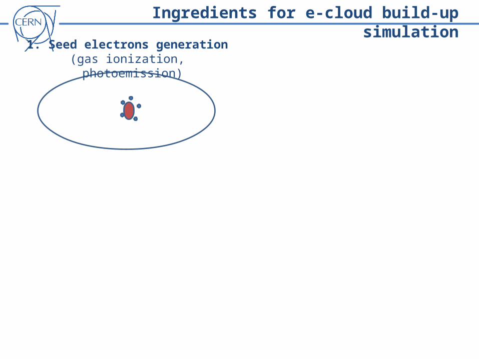
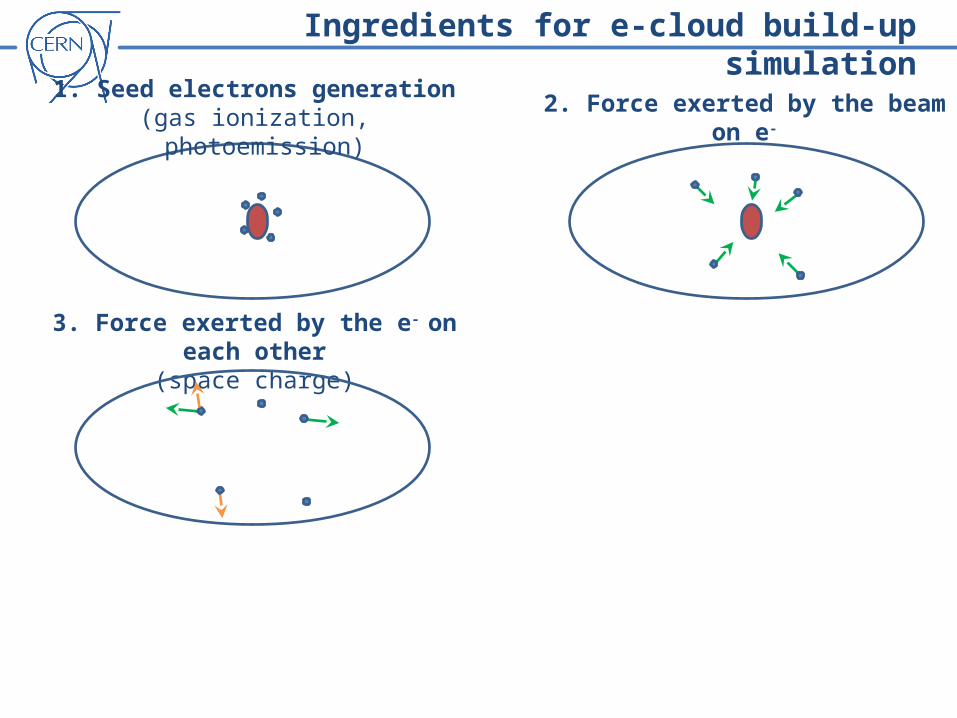
Ingredients for e-cloud build-up simulation
1. Seed electrons generation (gas ionization, photoemission)
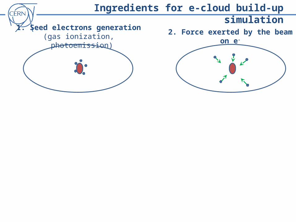
Ingredients for e-cloud build-up simulation
1. Seed electrons generation (gas ionization, photoemission) 2. Force exerted by the beam on e-
Ingredients for e-cloud build-up simulation
1. Seed electrons generation (gas ionization, photoemission) 2. Force exerted by the beam on e-
3. Force exerted by the e- on each other(space charge)
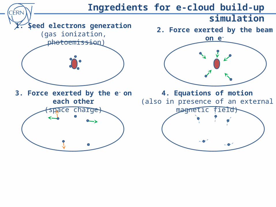
Ingredients for e-cloud build-up simulation
1. Seed electrons generation (gas ionization, photoemission) 2. Force exerted by the beam on e-
3. Force exerted by the e- on each other(space charge)
4. Equations of motion(also in presence of an external magnetic field)
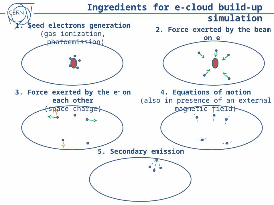
Ingredients for e-cloud build-up simulation
1. Seed electrons generation (gas ionization, photoemission) 2. Force exerted by the beam on e-
3. Force exerted by the e- on each other(space charge)
4. Equations of motion(also in presence of an external magnetic field)
5. Secondary emission
The most relevant improvements introduced in PyECLOUD are:
• A different management of macroparticle size and number
• A more accurate back-tracking algorithm for the impacting electrons
• A more efficient computation of the electric field generated by the
travelling proton beam
• A more general ad accurate method for the evaluation of the electrons
space-charge field
From ECLOUD to PyECLOUD
Outline
• Why a new code for electron cloud build-up simulation?
• From ECLOUD to PyECLOUD
o Management of macroparticle size and number
o Back-tracking algorithm for the impacting electrons
o Beam field calculation
o Space charge field
• Preliminary convergence study
• PyECLOUD at work
• Conclusion and future work
Macroparticles
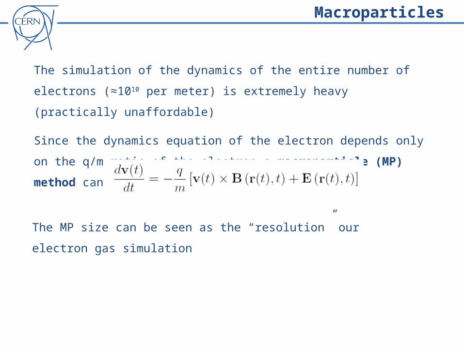
The simulation of the dynamics of the entire number of electrons (≈1010 per meter)
is extremely heavy (practically unaffordable)
Since the dynamics equation of the electron depends only on the q/m ratio of the
electron a macroparticle (MP) method can be used:
The MP size can be seen as the “resolution” our electron gas simulation
Macroparticles
0 1 2 3 4 5 6 7 8 9
x 10-6
104
106
108
time [s]Nu
mb
er
of e
- per
un
it le
ng
th [m
-1]
0 1 2 3 4 5 6 7 8 9
x 10-6
0
2
4
6
8x 10
11
time [s]Accu
m. n
um
ber
of scru
bb
. e- [
m-1
]
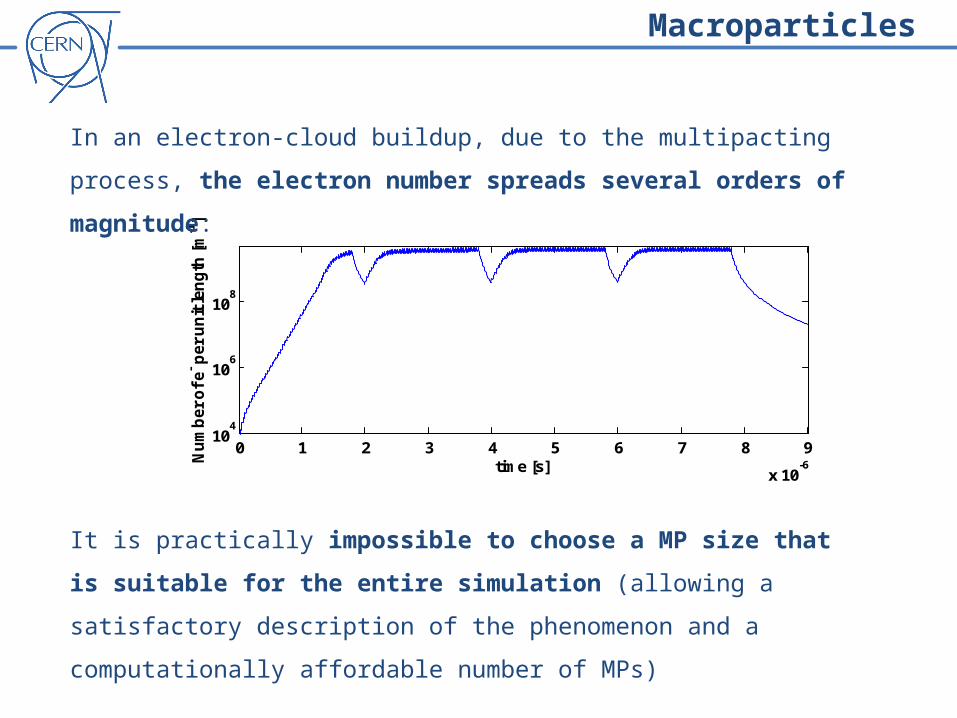
In an electron-cloud buildup, due to the multipacting process, the electron
number spreads several orders of magnitude:
It is practically impossible to choose a MP size that is suitable for the entire
simulation (allowing a satisfactory description of the phenomenon and a
computationally affordable number of MPs)
ECLOUD – MP number control: the CLEAN routine
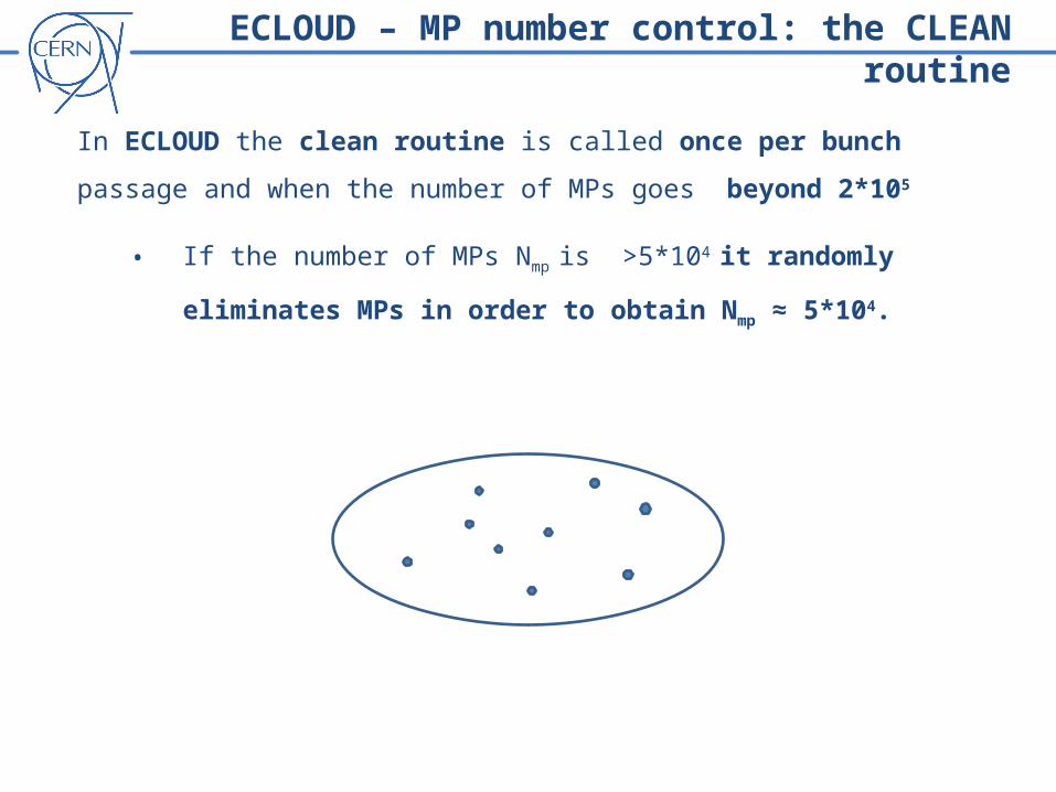
In ECLOUD the clean routine is called once per bunch passage and when the number
of MPs goes beyond 2*105

ECLOUD – MP number control: the CLEAN routine
In ECLOUD the clean routine is called once per bunch passage and when the number
of MPs goes beyond 2*105
• If the number of MPs Nmp is >5*104 it randomly eliminates MPs in order to
obtain Nmp ≈ 5*104.
ECLOUD – MP number control: the CLEAN routine
In ECLOUD the clean routine is called once per bunch passage and when the number
of MPs goes beyond 2*105
• If the number of MPs Nmp is >5*104 it randomly eliminates MPs in order to
obtain Nmp ≈ 5*104.
ECLOUD – MP number control: the CLEAN routine
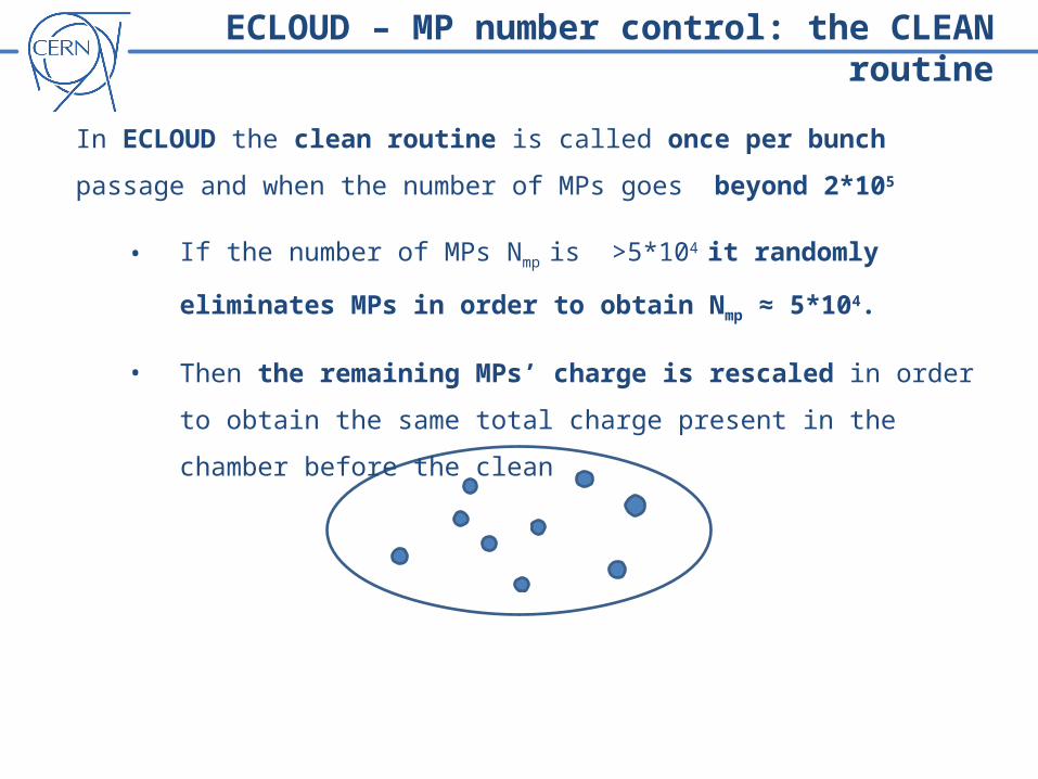
In ECLOUD the clean routine is called once per bunch passage and when the number
of MPs goes beyond 2*105
• If the number of MPs Nmp is >5*104 it randomly eliminates MPs in order to
obtain Nmp ≈ 5*104.
• Then the remaining MPs’ charge is rescaled in order to obtain the same
total charge present in the chamber before the clean
ECLOUD – MP number control: the CLEAN routine
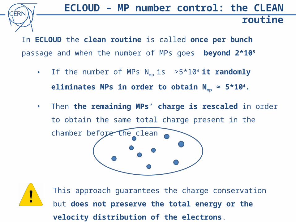
In ECLOUD the clean routine is called once per bunch passage and when the number
of MPs goes beyond 2*105
• If the number of MPs Nmp is >5*104 it randomly eliminates MPs in order to
obtain Nmp ≈ 5*104.
• Then the remaining MPs’ charge is rescaled in order to obtain the same
total charge present in the chamber before the clean
This approach guarantees the charge conservation but does not preserve
the total energy or the velocity distribution of the electrons.
In a typical ECLOUD simulation (SPS MBB SEY=1.5):
• The number and the size of MPs produced by the seed generation
mechanism is kept constant during the entire simulation.
As consequence, at saturation, we have a certain number of MPs
carrying practically no charge (≈ 5% of the MPs carries ≈1ppm of the
total charge)
ECLOUD – MP number control: other observations
In a typical ECLOUD simulation (SPS MBB SEY=1.5):
• The number and the size of MPs produced by the seed generation
mechanism is kept constant during the entire simulation.
As consequence, at saturation, we have a certain number of MPs
carrying practically no charge (≈ 5% of the MPs carries ≈1ppm of the
total charge)
• At saturation, there is a consistent number of MPs which are trapped
near the chamber wall and undergo several low energy impact becoming
smaller and smaller.
In ECLOUD there is no mechanism which selectively eliminates them.
ECLOUD – MP number control: other observations
In PyECLOUD we try to treat in a unified way all issues related to MP size and number,
namely:
PyECLOUD – MP number control: a global approach
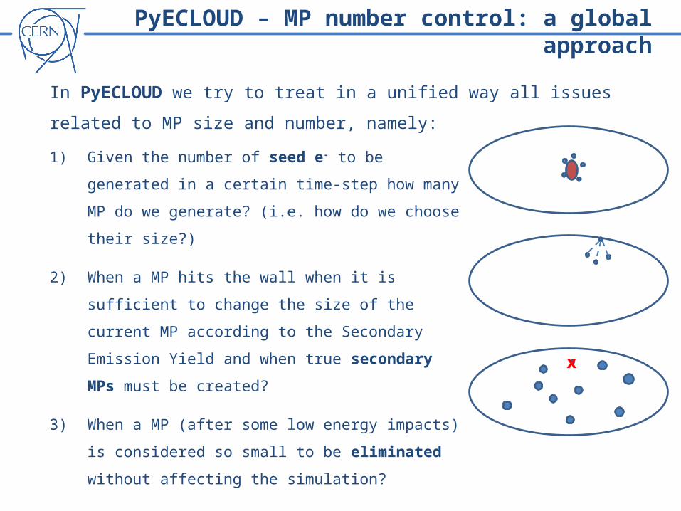
In PyECLOUD we try to treat in a unified way all issues related to MP size and number,
namely:
1) Given the number of seed e- to be generated in a certain
time-step how many MP do we generate? (i.e. how do we
choose their size?)
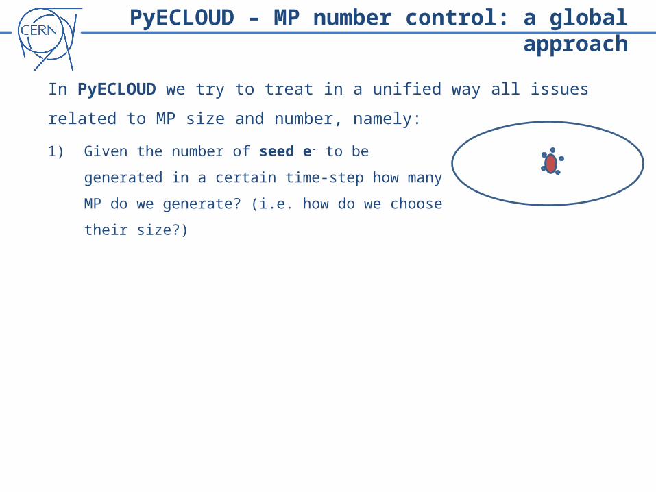
PyECLOUD – MP number control: a global approach
In PyECLOUD we try to treat in a unified way all issues related to MP size and number,
namely:
1) Given the number of seed e- to be generated in a certain
time-step how many MP do we generate? (i.e. how do we
choose their size?)
2) When a MP hits the wall when it is sufficient to change the
size of the current MP according to the Secondary Emission
Yield and when true secondary MPs must be created?
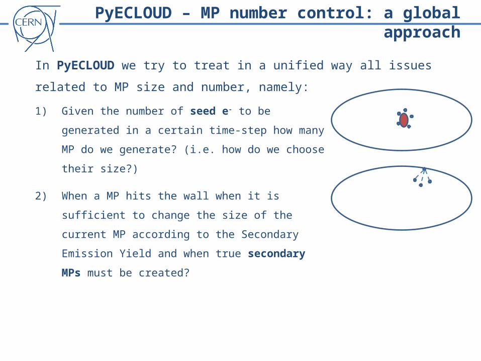
PyECLOUD – MP number control: a global approach

In PyECLOUD we try to treat in a unified way all issues related to MP size and number,
namely:
1) Given the number of seed e- to be generated in a certain
time-step how many MP do we generate? (i.e. how do we
choose their size?)
2) When a MP hits the wall when it is sufficient to change the
size of the current MP according to the Secondary Emission
Yield and when true secondary MPs must be created?
3) When a MP (after some low energy impacts) is considered so
small to be eliminated without affecting the simulation?
PyECLOUD – MP number control: a global approach
x
In PyECLOUD we try to treat in a unified way all issues related to MP size and number,
namely:
1) Given the number of seed e- to be generated in a certain
time-step how many MP do we generate? (i.e. how do we
choose their size?)
2) When a MP hits the wall when it is sufficient to change the
size of the current MP according to the Secondary Emission
Yield and when true secondary MPs must be created?
3) When a MP (after some low energy impacts) is considered so
small to be eliminated without affecting the simulation?
4) What to do when, because of multipacting process, the
number of MPs becomes too large for a reasonable
computational burden ?
PyECLOUD – MP number control: a global approach
x
We control all this issues through the single parameter Nref which is a target average size
of the MPs (i.e. our resolution) and is adaptively changed during the simulation:
PyECLOUD – MP number control: a global approach
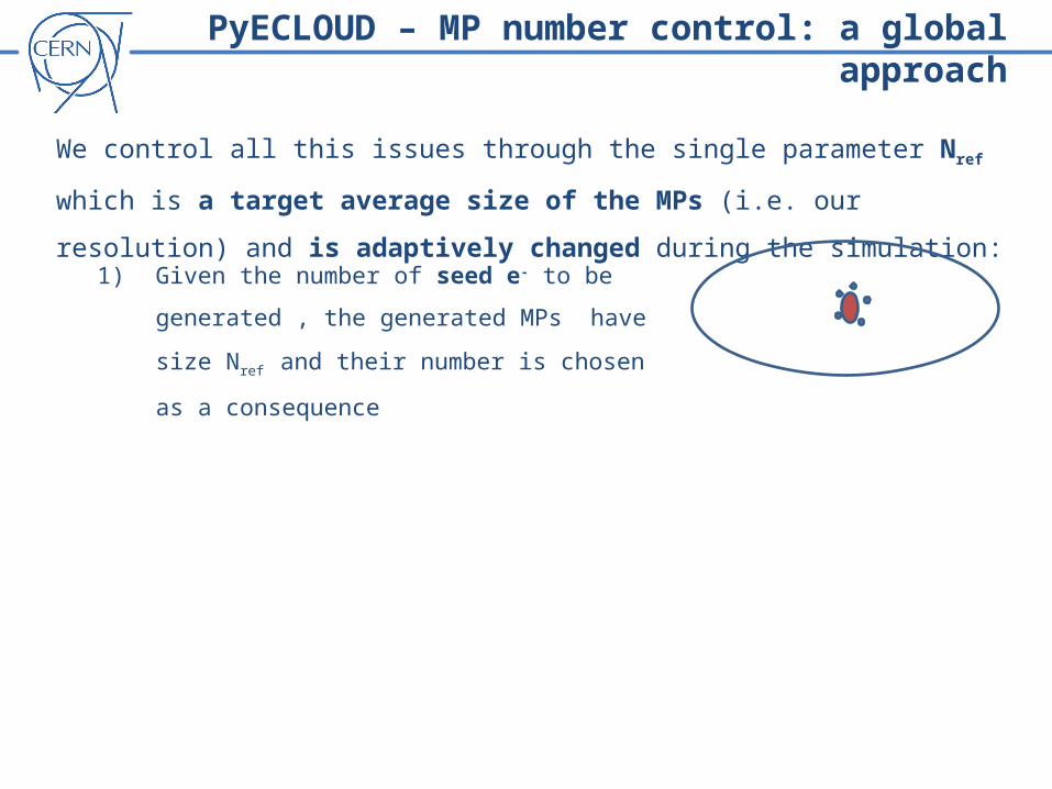
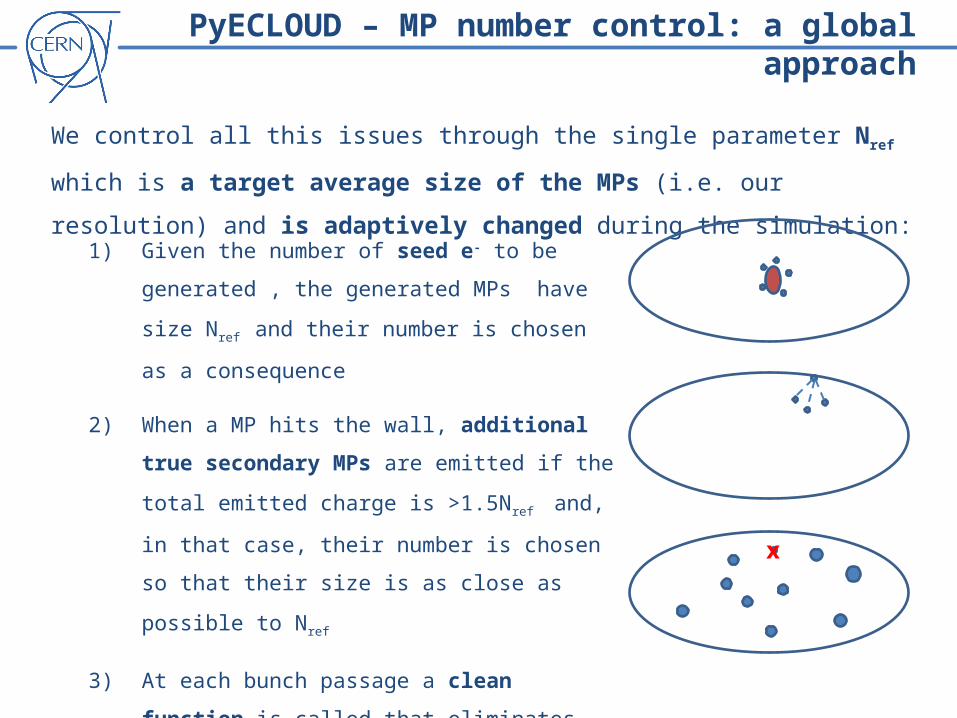
We control all this issues through the single parameter Nref which is a target average size
of the MPs (i.e. our resolution) and is adaptively changed during the simulation:
1) Given the number of seed e- to be generated , the
generated MPs have size Nref and their number is
chosen as a consequence
PyECLOUD – MP number control: a global approach
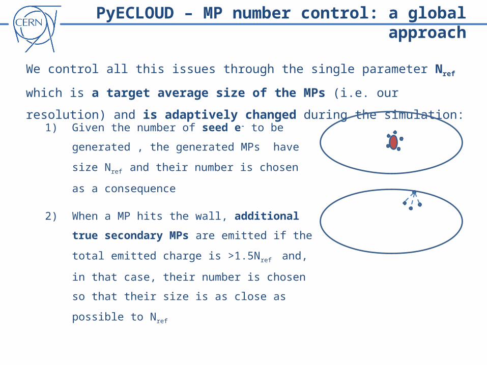
We control all this issues through the single parameter Nref which is a target average size
of the MPs (i.e. our resolution) and is adaptively changed during the simulation:
1) Given the number of seed e- to be generated , the
generated MPs have size Nref and their number is
chosen as a consequence
2) When a MP hits the wall, additional true secondary
MPs are emitted if the total emitted charge is >1.5Nref
and, in that case, their number is chosen so that their
size is as close as possible to Nref
PyECLOUD – MP number control: a global approach
We control all this issues through the single parameter Nref which is a target average size
of the MPs (i.e. our resolution) and is adaptively changed during the simulation:
1) Given the number of seed e- to be generated , the
generated MPs have size Nref and their number is
chosen as a consequence
2) When a MP hits the wall, additional true secondary
MPs are emitted if the total emitted charge is >1.5Nref
and, in that case, their number is chosen so that their
size is as close as possible to Nref
3) At each bunch passage a clean function is called that
eliminates all the MPs with charge <10-4Nref
x
PyECLOUD – MP number control: a global approach
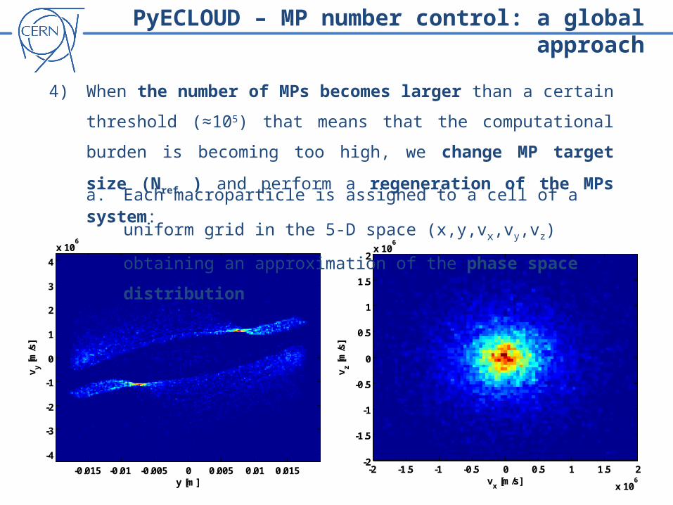
4) When the number of MPs becomes larger than a certain threshold (≈105)
that means that the computational burden is becoming too high, we change
MP target size (Nref ) and perform a regeneration of the MPs system:
PyECLOUD – MP number control: a global approach
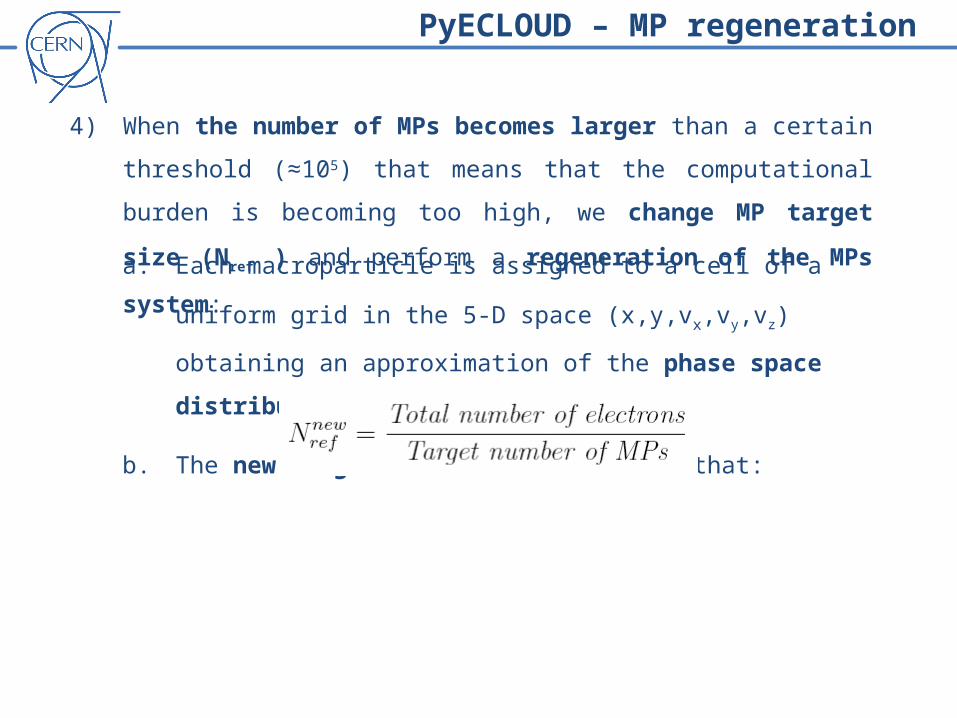
4) When the number of MPs becomes larger than a certain threshold (≈105)
that means that the computational burden is becoming too high, we change
MP target size (Nref ) and perform a regeneration of the MPs system:
a. Each macroparticle is assigned to a cell of a uniform grid in the 5-D space
(x,y,vx,vy,vz) obtaining an approximation of the phase space distribution
PyECLOUD – MP number control: a global approach
x [m]
y [
m]
-0.02 -0.01 0 0.01 0.02
-0.015
-0.01
-0.005
0
0.005
0.01
0.015
x [m]
vx [
m/s
]
-0.02 -0.015 -0.01 -0.005 0 0.005 0.01 0.015 0.02
-4
-3
-2
-1
0
1
2
3
4
x 106
y [m]
vy [
m/s
]
-0.015 -0.01 -0.005 0 0.005 0.01 0.015
-4
-3
-2
-1
0
1
2
3
4
x 106
vx [m/s]
vz [
m/s
]
-2 -1.5 -1 -0.5 0 0.5 1 1.5 2
x 106
-2
-1.5
-1
-0.5
0
0.5
1
1.5
2x 10
6
4) When the number of MPs becomes larger than a certain threshold (≈105)
that means that the computational burden is becoming too high, we change
MP target size (Nref ) and perform a regeneration of the MPs system:
a. Each macroparticle is assigned to a cell of a uniform grid in the 5-D space
(x,y,vx,vy,vz) obtaining an approximation of the phase space distribution
PyECLOUD – MP number control: a global approach
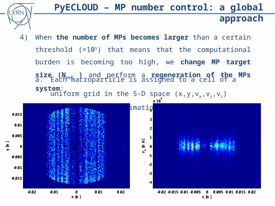
4) When the number of MPs becomes larger than a certain threshold (≈105)
that means that the computational burden is becoming too high, we change
MP target size (Nref ) and perform a regeneration of the MPs system:
a. Each macroparticle is assigned to a cell of a uniform grid in the 5-D space
(x,y,vx,vy,vz) obtaining an approximation of the phase space distribution
b. The new target MP size is chosen so that:
PyECLOUD – MP regeneration
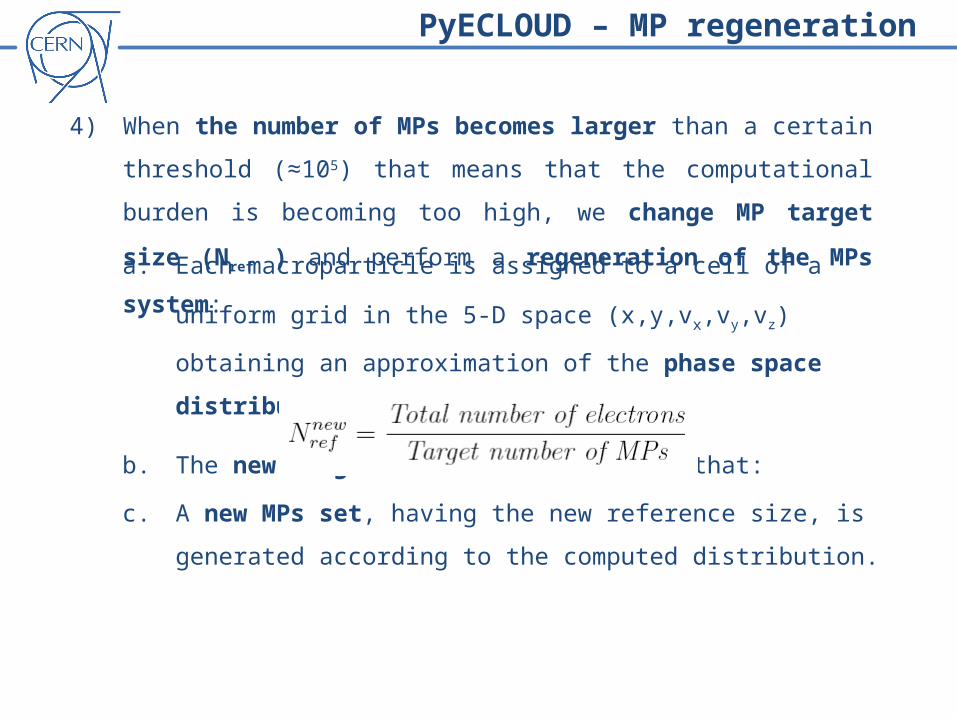
4) When the number of MPs becomes larger than a certain threshold (≈105)
that means that the computational burden is becoming too high, we change
MP target size (Nref ) and perform a regeneration of the MPs system:
a. Each macroparticle is assigned to a cell of a uniform grid in the 5-D space
(x,y,vx,vy,vz) obtaining an approximation of the phase space distribution
b. The new target MP size is chosen so that:
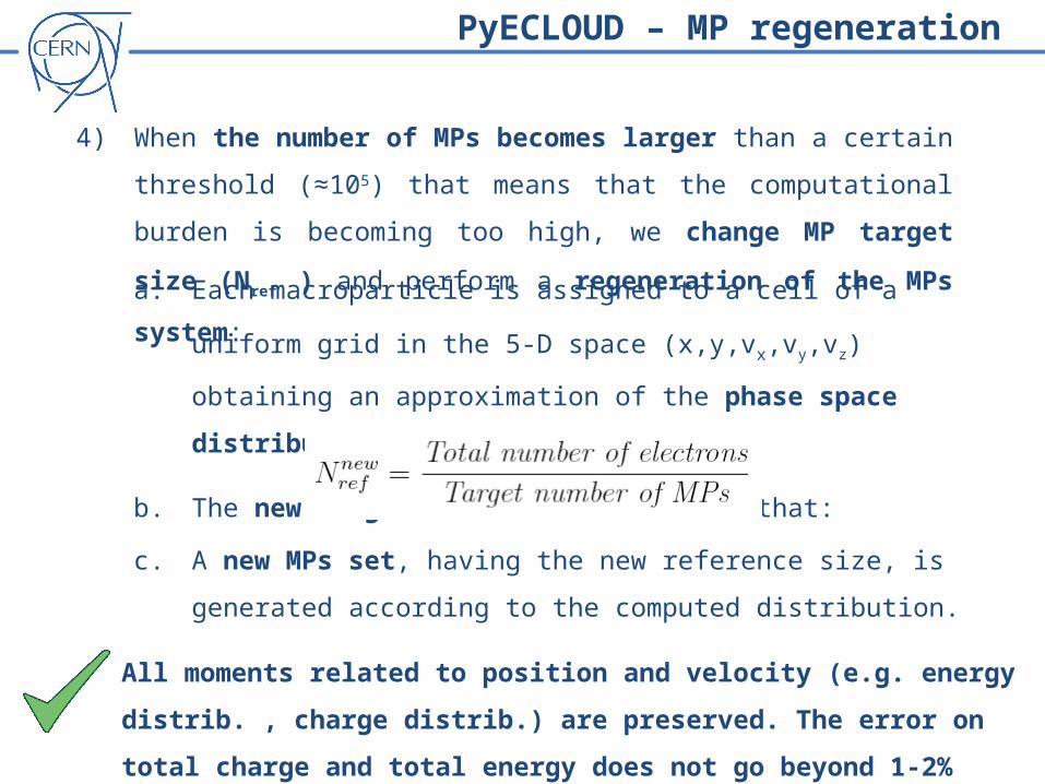
c. A new MPs set, having the new reference size, is generated according to
the computed distribution.
PyECLOUD – MP regeneration
4) When the number of MPs becomes larger than a certain threshold (≈105)
that means that the computational burden is becoming too high, we change
MP target size (Nref ) and perform a regeneration of the MPs system:
a. Each macroparticle is assigned to a cell of a uniform grid in the 5-D space
(x,y,vx,vy,vz) obtaining an approximation of the phase space distribution
b. The new target MP size is chosen so that:
c. A new MPs set, having the new reference size, is generated according to
the computed distribution.
PyECLOUD – MP regeneration
All moments related to position and velocity (e.g. energy distrib. , charge distrib.)
are preserved. The error on total charge and total energy does not go beyond 1-2%
Outline
• Why a new code for electron cloud build-up simulation?
• From ECLOUD to PyECLOUD
o Management of macroparticle size and number
o Back-tracking algorithm for the impacting electrons
o Beam field calculation
o Space charge field
• Preliminary convergence study
• PyECLOUD at work
• Conclusion and future work
Impacting electrons backtracking - ECLOUD
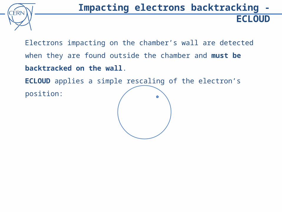
Electrons impacting on the chamber’s wall are detected when they are found outside
the chamber and must be backtracked on the wall.
ECLOUD applies a simple rescaling of the electron’s position:
Impacting electrons backtracking - ECLOUD
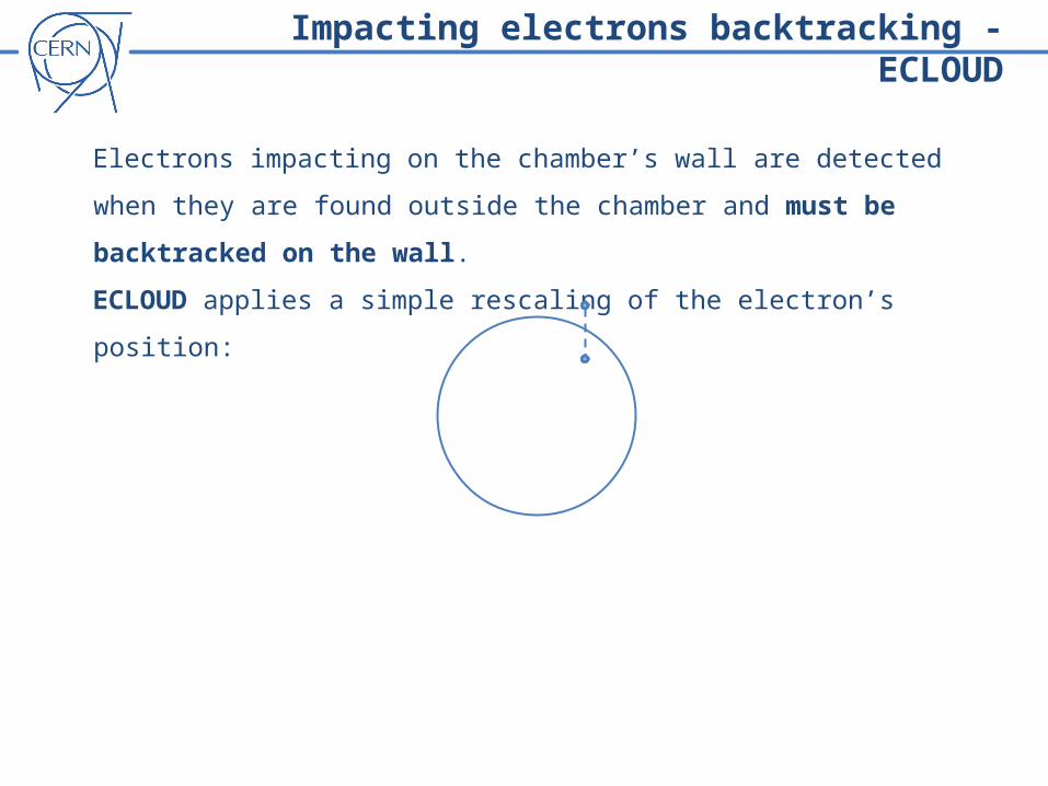
Electrons impacting on the chamber’s wall are detected when they are found outside
the chamber and must be backtracked on the wall.
ECLOUD applies a simple rescaling of the electron’s position:
Impacting electrons backtracking - ECLOUD
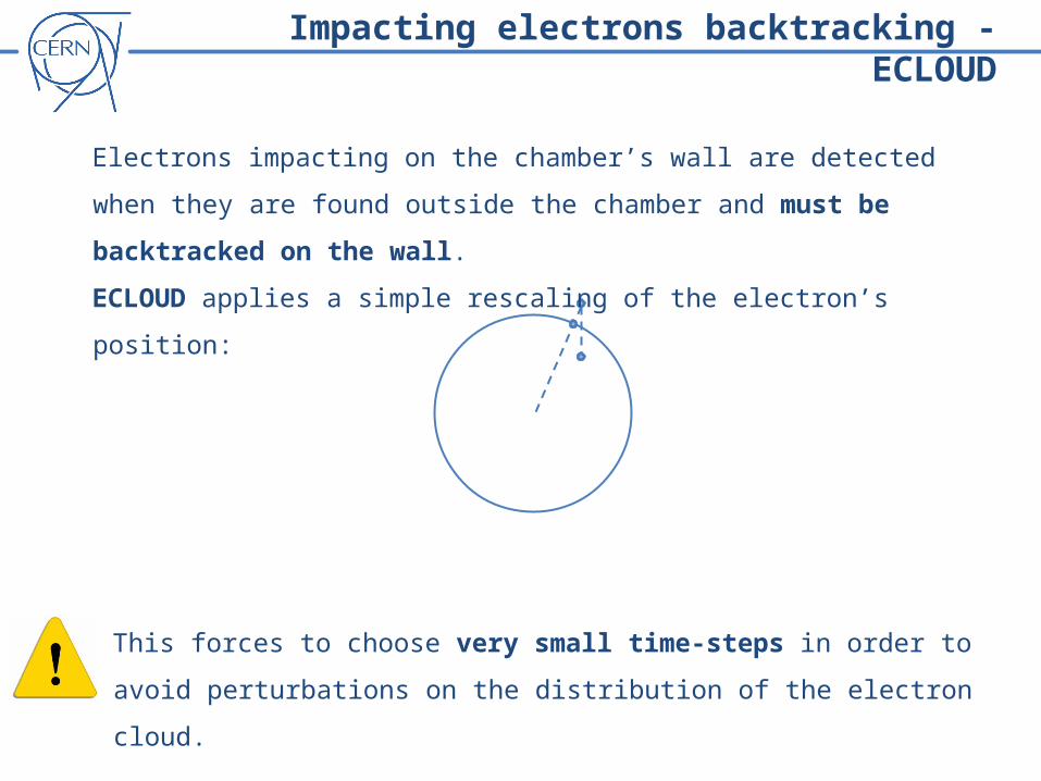
Electrons impacting on the chamber’s wall are detected when they are found outside
the chamber and must be backtracked on the wall.
ECLOUD applies a simple rescaling of the electron’s position:
This forces to choose very small time-steps in order to avoid perturbations on the
distribution of the electron cloud.

Impacting electrons backtracking - PyECLOUD
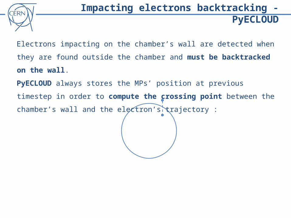
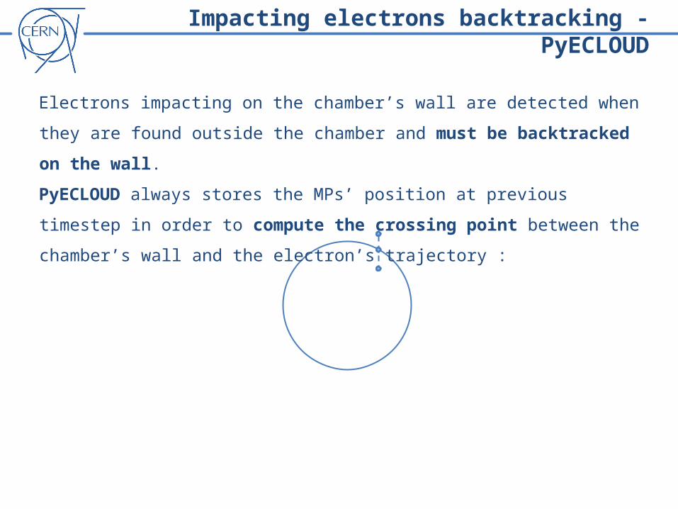
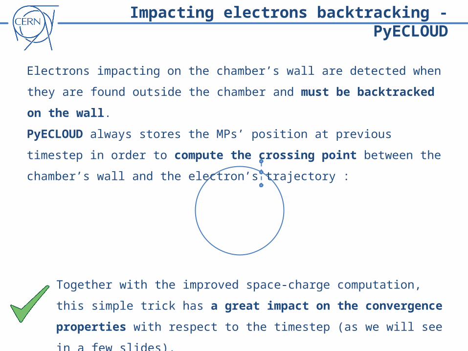
Electrons impacting on the chamber’s wall are detected when they are found outside the
chamber and must be backtracked on the wall.
PyECLOUD always stores the MPs’ position at previous timestep in order to compute the
crossing point between the chamber’s wall and the electron’s trajectory :
Impacting electrons backtracking - PyECLOUD
Electrons impacting on the chamber’s wall are detected when they are found outside the
chamber and must be backtracked on the wall.
PyECLOUD always stores the MPs’ position at previous timestep in order to compute the
crossing point between the chamber’s wall and the electron’s trajectory :
Together with the improved space-charge computation, this simple trick has a
great impact on the convergence properties with respect to the timestep (as we
will see in a few slides).
Outline
• Why a new code for electron cloud build-up simulation?
• From ECLOUD to PyECLOUD
o Management of macroparticle size and number
o Back-tracking algorithm for the impacting electrons
o Beam field calculation
o Space charge field
• Preliminary convergence study
• PyECLOUD at work
• Conclusion and future work
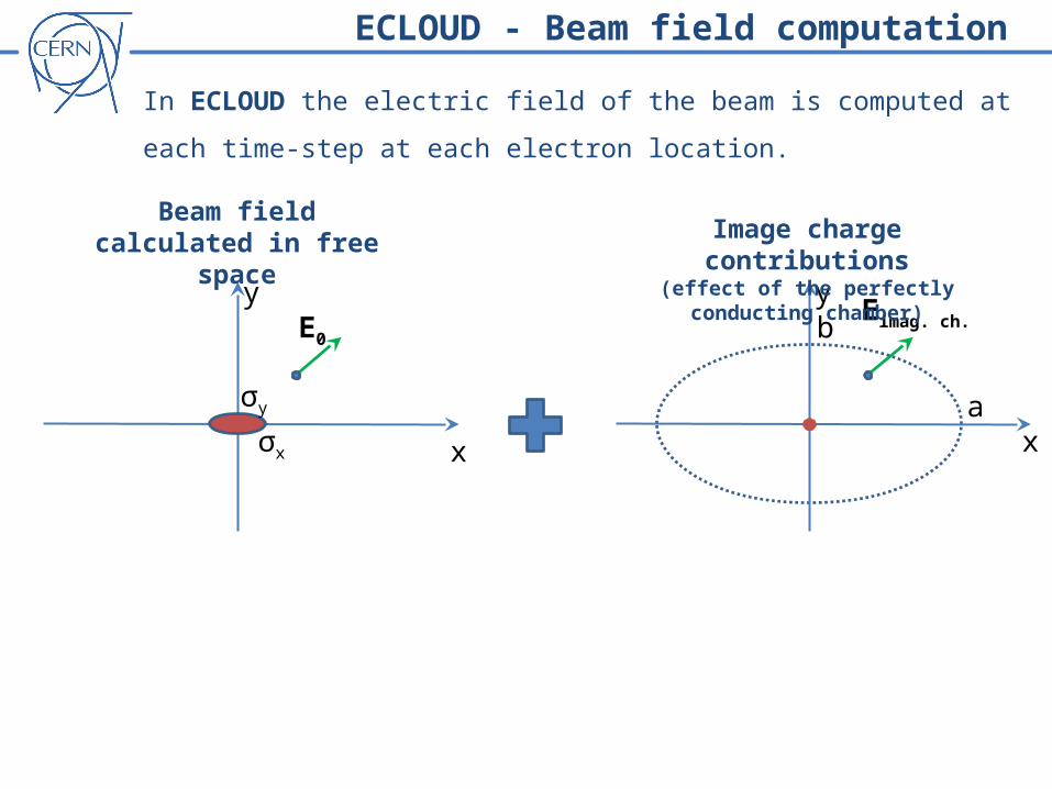
ECLOUD - Beam field computation
In ECLOUD the electric field of the beam is computed at each time-step at each
electron location.
x
y
σy
σx
E0 b
ax
y Eimag. ch.
Beam fieldcalculated in free space Image charge contributions
(effect of the perfectly conducting chamber)
In ECLOUD the electric field of the beam is computed at each time-step at each
electron location.
x
y
σy
σx
E0 b
ax
y Eimag. ch.
Beam fieldcalculated in free space Image charge contributions
(effect of the perfectly conducting chamber)
2
20 0
2( , ) ( , )x y
i zE x y iE x y e w w
S S S
2 22 x yS y x
x y
x i y
x y
x yi
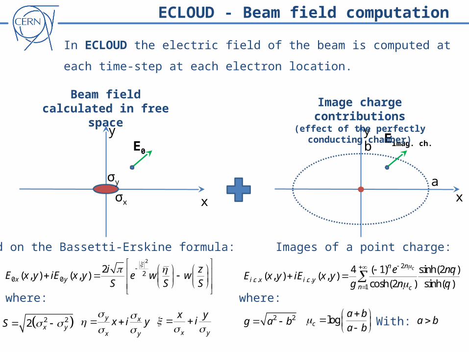
Based on the Bassetti-Erskine formula: Images of a point charge:2
. . . .1
4 ( 1) sinh(2 )( , ) ( , )
cosh(2 ) sinh( )
cnn
i c x i c yn c
e nqE x y iE x y
g n q
where: where:
2 2g a b logca b
a b
With: a b
ECLOUD - Beam field computation
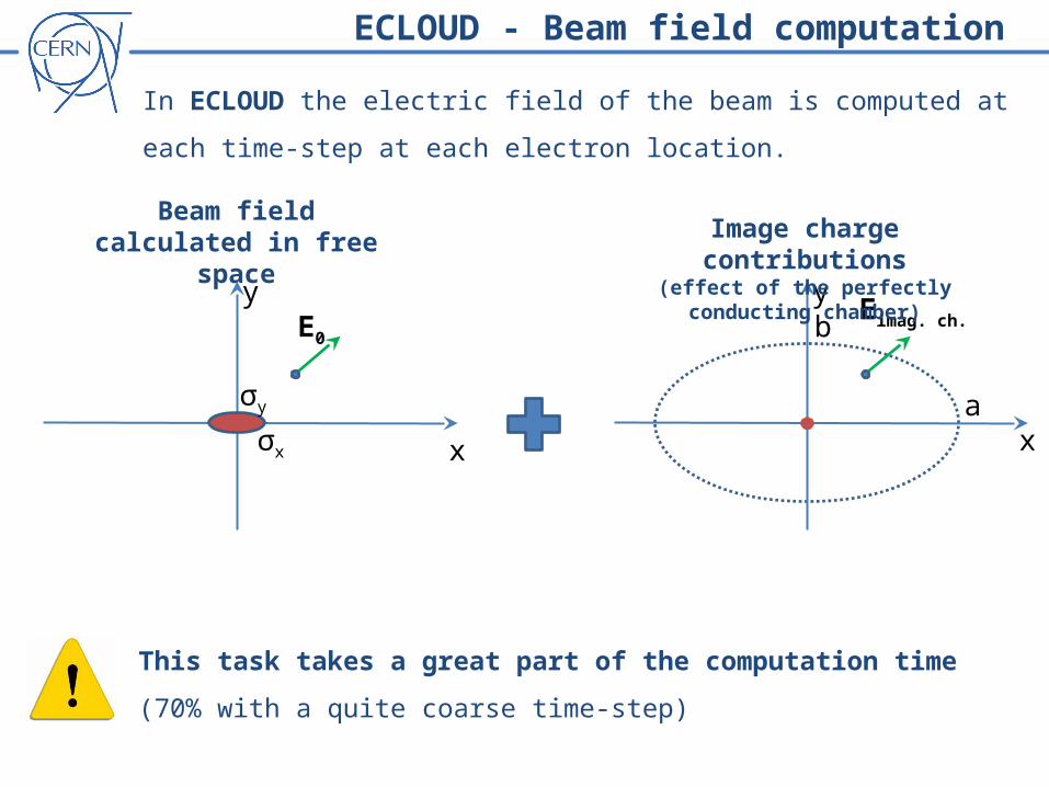
In ECLOUD the electric field of the beam is computed at each time-step at each
electron location.
x
y
σy
σx
E0 b
ax
y Eimag. ch.
Beam fieldcalculated in free space Image charge contributions
(effect of the perfectly conducting chamber)
This task takes a great part of the computation time (70% with a quite coarse
time-step)
ECLOUD - Beam field computation
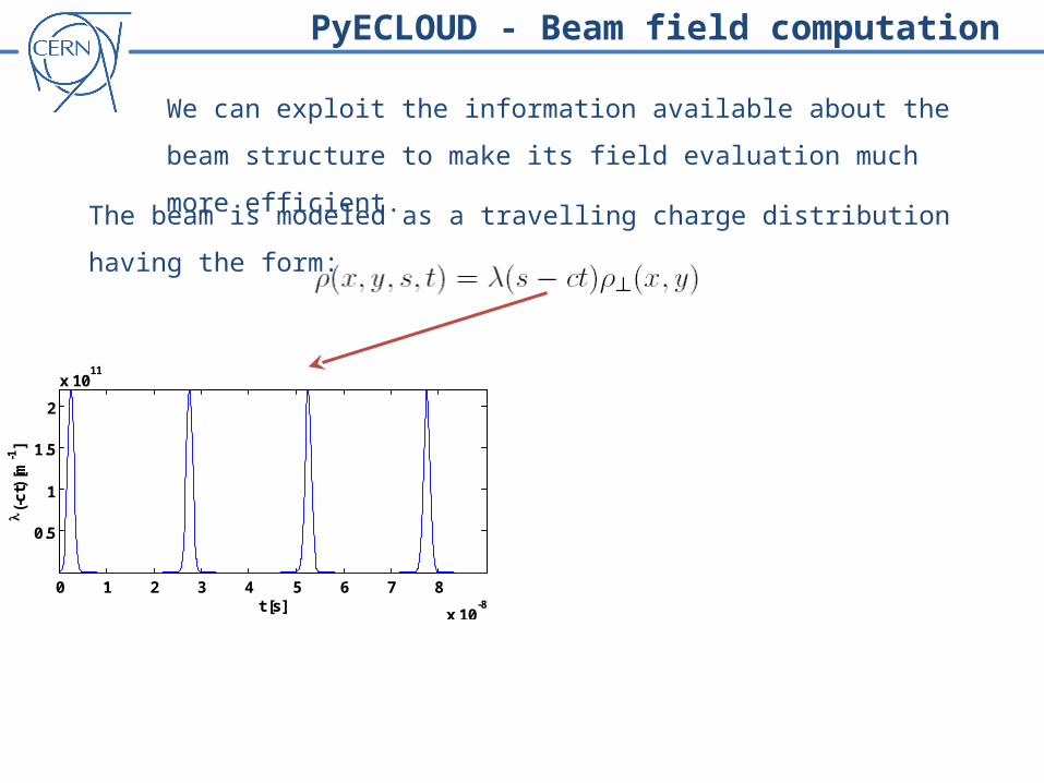
We can exploit the information available about the beam structure to make
its field evaluation much more efficient.
The beam is modeled as a travelling charge distribution having the form:
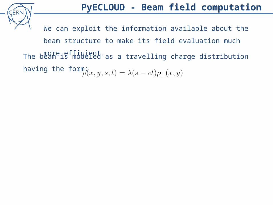
PyECLOUD - Beam field computation
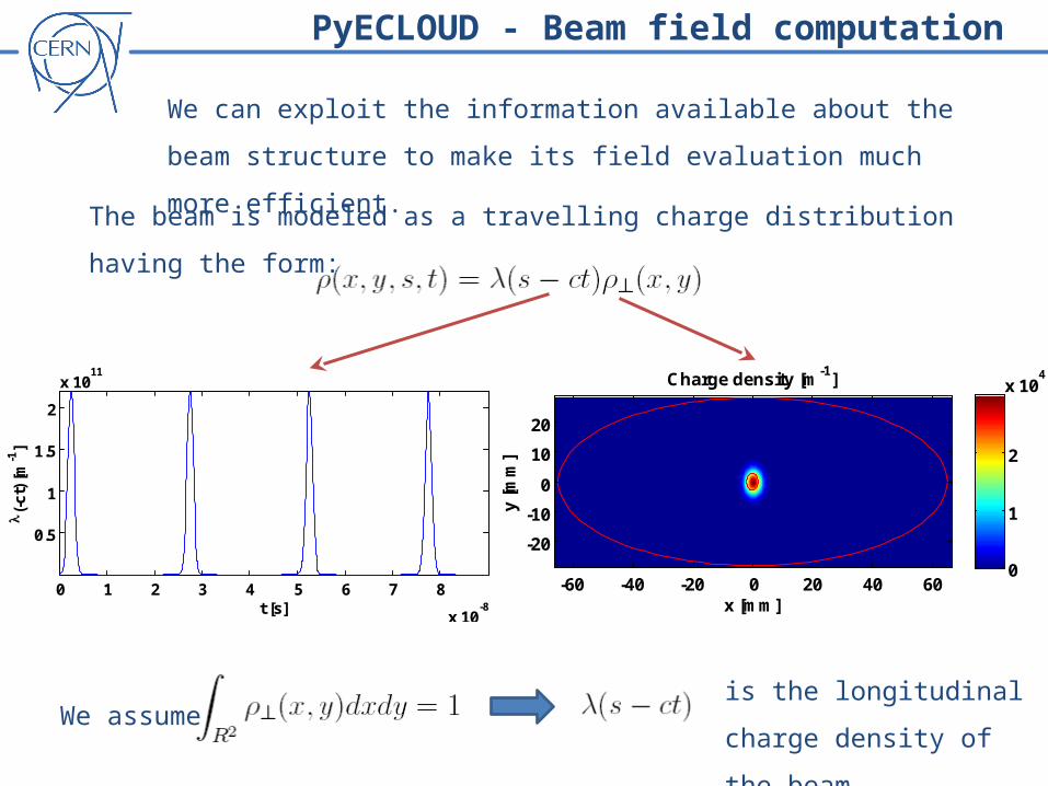
We can exploit the information available about the beam structure to make
its field evaluation much more efficient.
The beam is modeled as a travelling charge distribution having the form:
0 1 2 3 4 5 6 7 8
x 10-8
0.5
1
1.5
2
x 1011
t [s]
(-
ct)
[m
-1]
PyECLOUD - Beam field computation
We can exploit the information available about the beam structure to make
its field evaluation much more efficient.
The beam is modeled as a travelling charge distribution having the form:
x [mm]
y [
mm
]
Charge density [m-1]
-60 -40 -20 0 20 40 60
-20
-10
0
10
20
0
1
2
x 104
0 1 2 3 4 5 6 7 8
x 10-8
0.5
1
1.5
2
x 1011
t [s]
(-
ct)
[m
-1]
We assumeis the longitudinal charge
density of the beam
PyECLOUD - Beam field computation
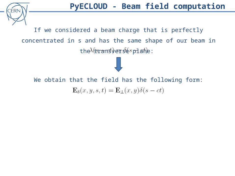
If we considered a beam charge that is perfectly concentrated in s and has the same
shape of our beam in the transverse plane:
We obtain that the field has the following form:
PyECLOUD - Beam field computation
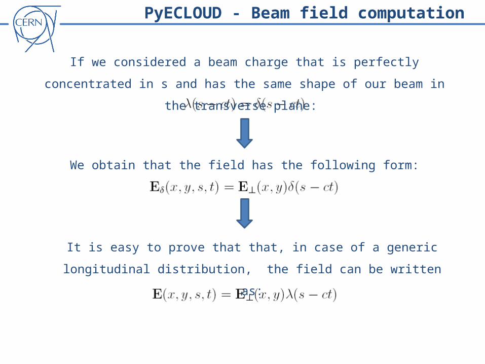
If we considered a beam charge that is perfectly concentrated in s and has the same
shape of our beam in the transverse plane:
We obtain that the field has the following form:
It is easy to prove that that, in case of a generic longitudinal distribution, the
field can be written as:
PyECLOUD - Beam field computation
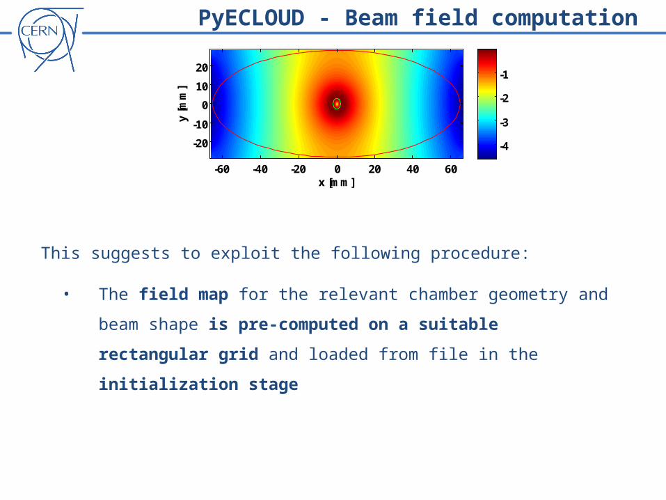
x [mm]y
[m
m]
E log(normalizad magnitude) - with image charges
-60 -40 -20 0 20 40 60
-20
-10
0
10
20
-4
-3
-2
-1
This suggests to exploit the following procedure:
• The field map for the relevant chamber geometry and beam shape is pre-
computed on a suitable rectangular grid and loaded from file in the
initialization stage
PyECLOUD - Beam field computation
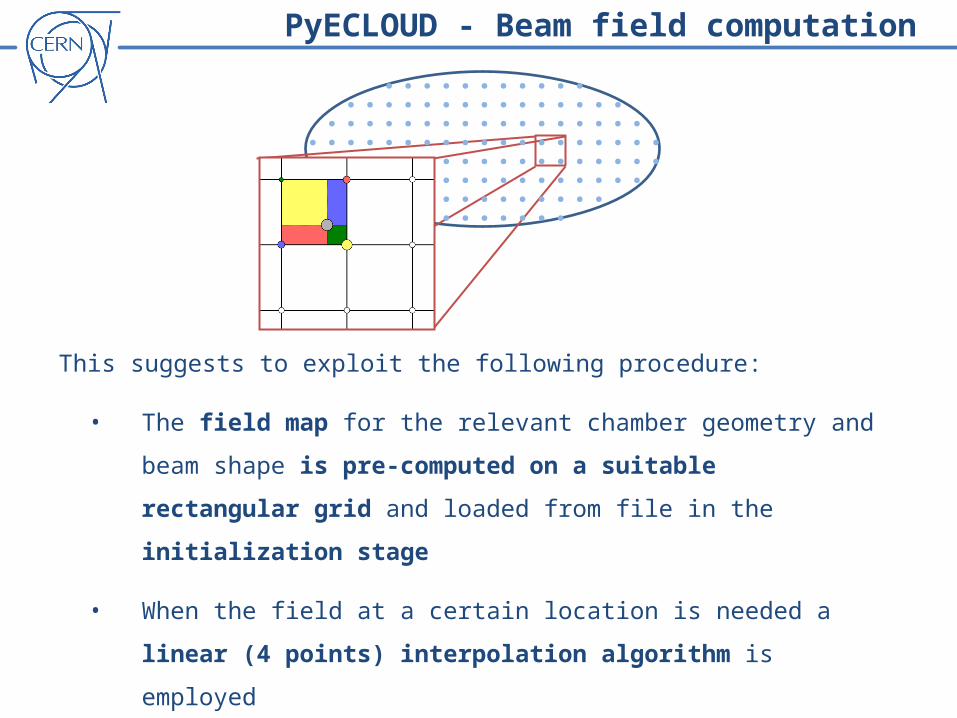
This suggests to exploit the following procedure:
• The field map for the relevant chamber geometry and beam shape is pre-
computed on a suitable rectangular grid and loaded from file in the
initialization stage
• When the field at a certain location is needed a linear (4 points)
interpolation algorithm is employed
PyECLOUD - Beam field computation
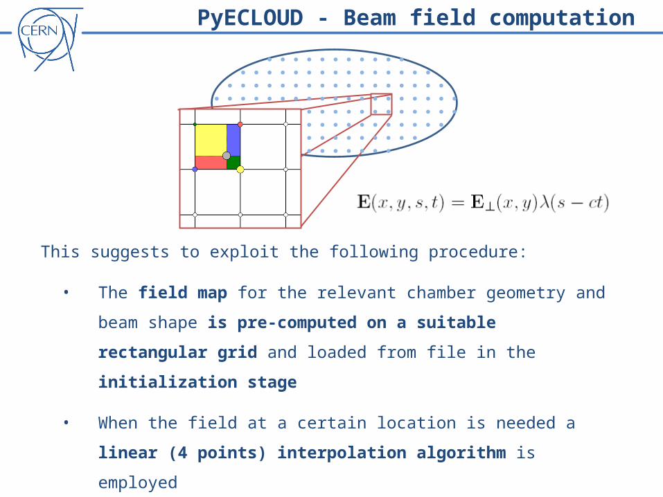
This suggests to exploit the following procedure:
• The field map for the relevant chamber geometry and beam shape is pre-
computed on a suitable rectangular grid and loaded from file in the
initialization stage
• When the field at a certain location is needed a linear (4 points)
interpolation algorithm is employed
• The field is rescaled by the relevant beam longitudinal density
PyECLOUD - Beam field computation
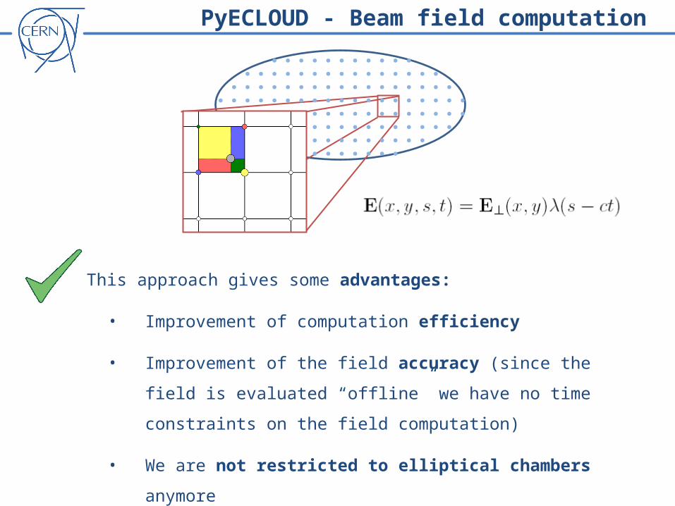
This approach gives some advantages:
• Improvement of computation efficiency
• Improvement of the field accuracy (since the field is evaluated “offline”
we have no time constraints on the field computation)
• We are not restricted to elliptical chambers anymore
PyECLOUD - Beam field computation
Outline
• Why a new code for electron cloud build-up simulation?
• From ECLOUD to PyECLOUD
o Management of macroparticle size and number
o Back-tracking algorithm for the impacting electrons
o Beam field calculation
o Space charge field
• Preliminary convergence study
• PyECLOUD at work
• Conclusion and future work
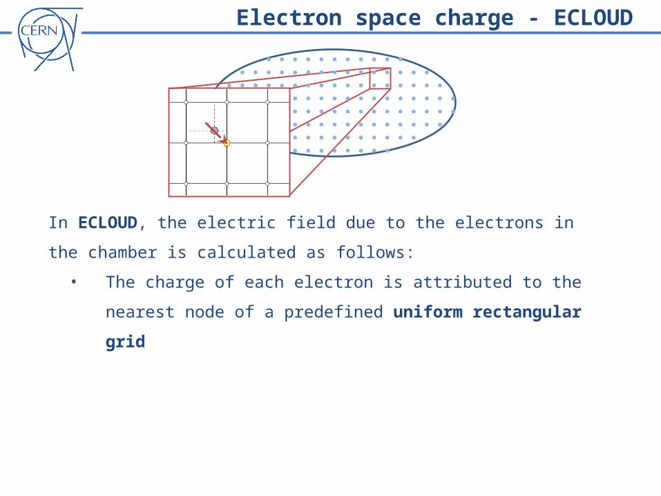
Electron space charge - ECLOUD
In ECLOUD, the electric field due to the electrons in the chamber is calculated as
follows:
• The charge of each electron is attributed to the nearest node of a
predefined uniform rectangular grid
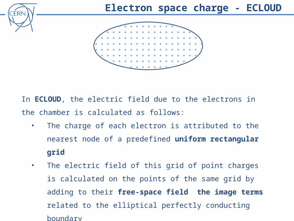
Electron space charge - ECLOUD
In ECLOUD, the electric field due to the electrons in the chamber is calculated as
follows:
• The charge of each electron is attributed to the nearest node of a
predefined uniform rectangular grid
• The electric field of this grid of point charges is calculated on the points
of the same grid by adding to their free-space field the image terms
related to the elliptical perfectly conducting boundary
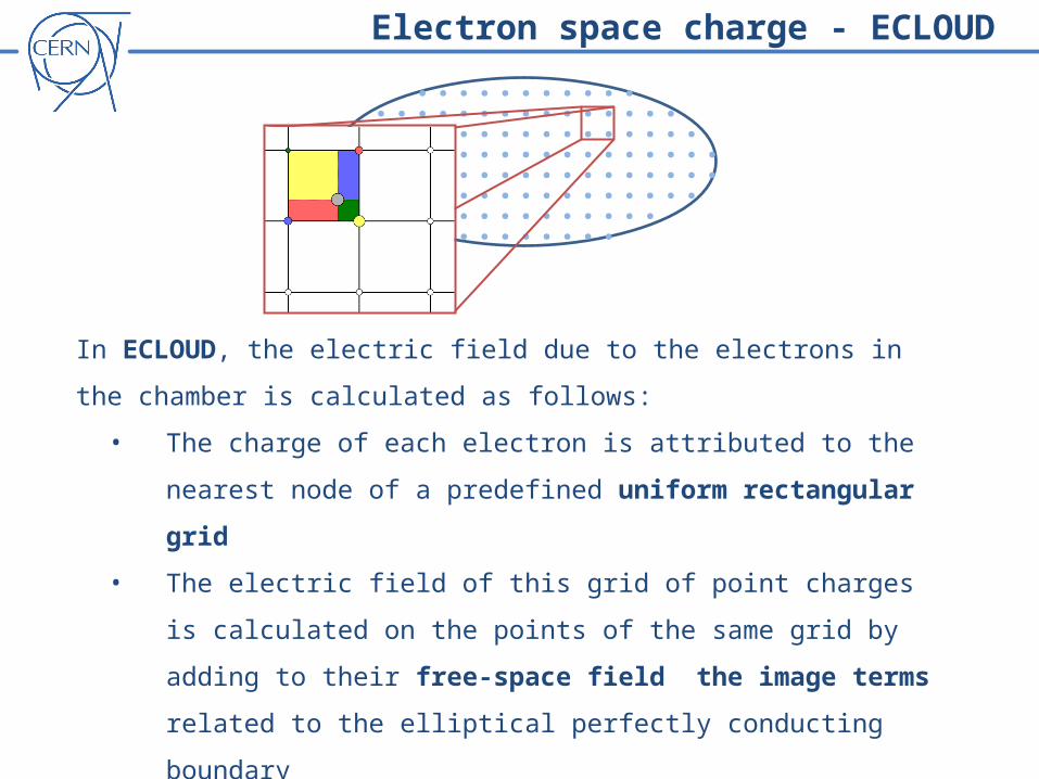
• The electric field at the location of each electron is evaluated employing
a linear (4-point) interpolation formula
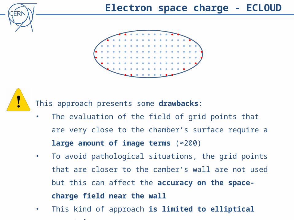
Electron space charge - ECLOUD
This approach presents some drawbacks:
• The evaluation of the field of grid points that are very close to the
chamber’s surface require a large amount of image terms (≈200)
• To avoid pathological situations, the grid points that are closer to the
camber’s wall are not used but this can affect the accuracy on the space-
charge field near the wall
• This kind of approach is limited to elliptical geometries
Electron space charge - PyECLOUD
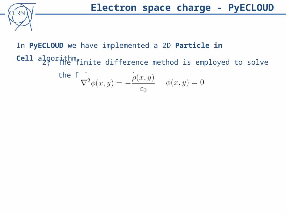
In PyECLOUD we have implemented a 2D Particle in Cell algorithm.
• The electrostatic potential in the chamber is solution of the Poisson equation
with homogeneous boundary conditions:
with on the boundary
Electrostatic potential Electron charge density
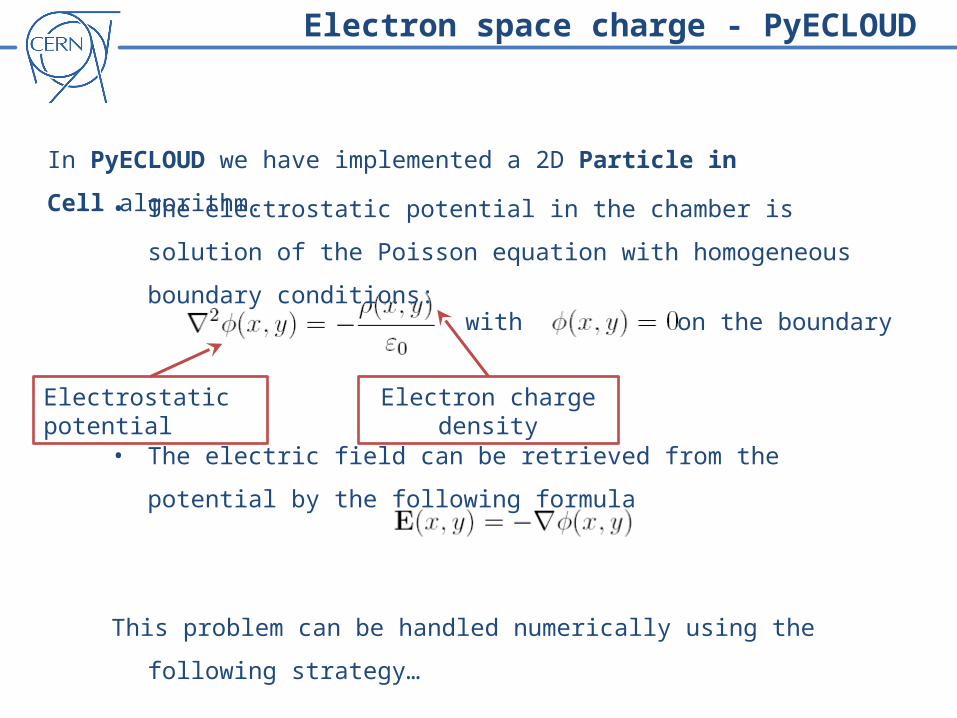
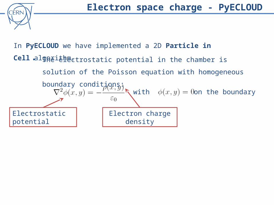
Electron space charge - PyECLOUD
In PyECLOUD we have implemented a 2D Particle in Cell algorithm.
• The electrostatic potential in the chamber is solution of the Poisson equation
with homogeneous boundary conditions:
with on the boundary
• The electric field can be retrieved from the potential by the following formula
Electrostatic potential Electron charge density
This problem can be handled numerically using the following strategy…
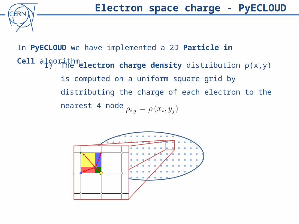
Electron space charge - PyECLOUD
In PyECLOUD we have implemented a 2D Particle in Cell algorithm.
1) The electron charge density distribution ρ(x,y) is computed on a uniform
square grid by distributing the charge of each electron to the nearest 4
nodes:
Electron space charge - PyECLOUD
In PyECLOUD we have implemented a 2D Particle in Cell algorithm.
2) The finite difference method is employed to solve the Poisson equation:
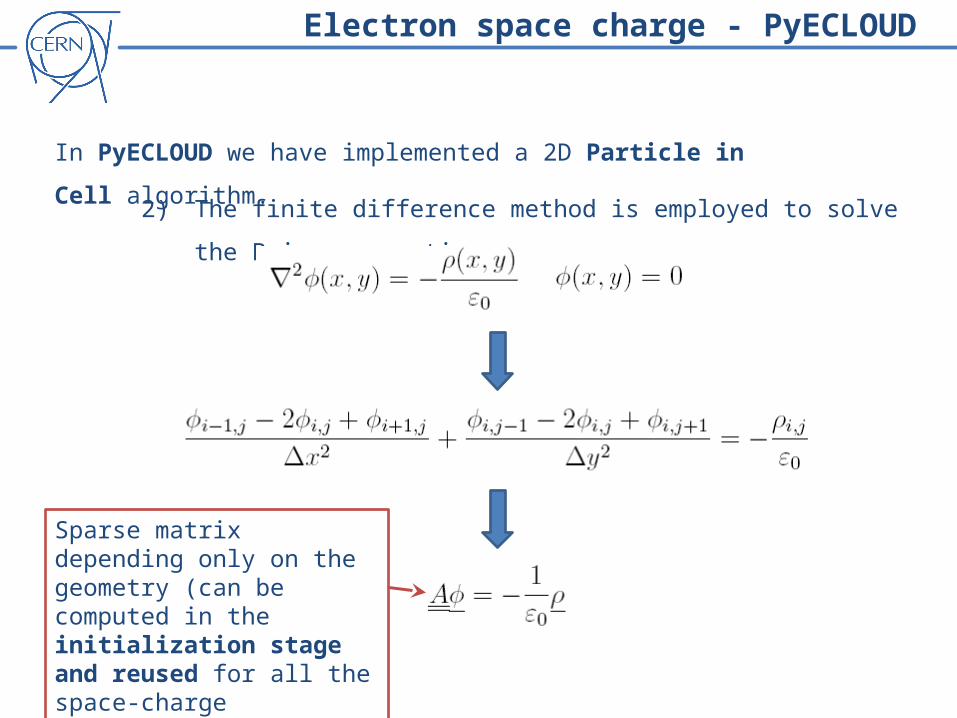
Electron space charge - PyECLOUD
In PyECLOUD we have implemented a 2D Particle in Cell algorithm.
2) The finite difference method is employed to solve the Poisson equation:
Sparse matrix depending only on the geometry (can be computed in the initialization stage and reused for all the space-charge evaluations).
Electron space charge - PyECLOUD
In PyECLOUD we have implemented a 2D Particle in Cell algorithm.
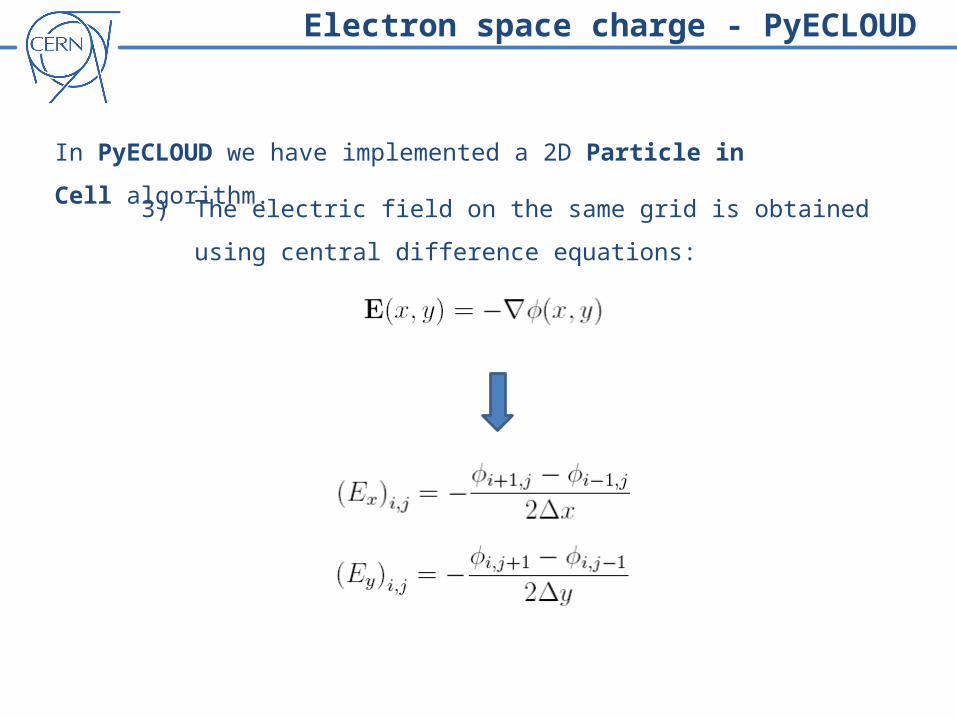
3) The electric field on the same grid is obtained using central difference
equations:
Electron space charge - PyECLOUD
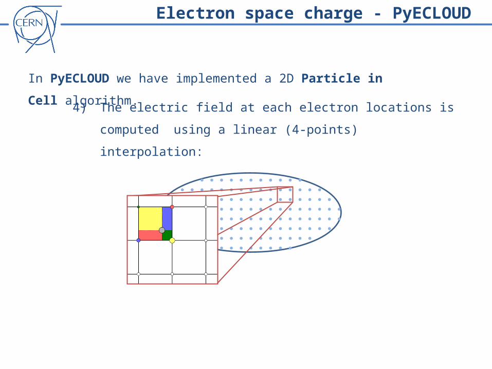
In PyECLOUD we have implemented a 2D Particle in Cell algorithm.
4) The electric field at each electron locations is computed using a linear (4-
points) interpolation:
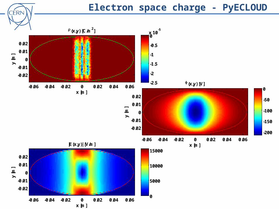
Electron space charge - PyECLOUD
x [m]
y [
m]
(x,y) [C/m2]
-0.06 -0.04 -0.02 0 0.02 0.04 0.06
-0.02
-0.01
0
0.01
0.02
-2.5
-2
-1.5
-1
-0.5
0x 10
-5
x [m]
y [
m]
(x,y) [V]
-0.06 -0.04 -0.02 0 0.02 0.04 0.06
-0.02
-0.01
0
0.01
0.02
-200
-150
-100
-50
0
x [m]
y [
m]
|E(x,y)| [V/m]
-0.06 -0.04 -0.02 0 0.02 0.04 0.06
-0.02
-0.01
0
0.01
0.02
0
5000
10000
15000
Electron space charge - PyECLOUD
In PyECLOUD we have implemented a 2D Particle in Cell algorithm.
This eliminates the convergence problems related to the image-
charge approach and also eliminates the limitation to geometries for
which image the charge expansion exists.
Outline
• Why a new code for electron cloud build-up simulation?
• From ECLOUD to PyECLOUD
o Management of macroparticle size and number
o back-tracking algorithm for the impacting electrons
o Beam field calculation
o Space charge field
• Preliminary convergence study
• PyECLOUD at work
• Conclusion and future work
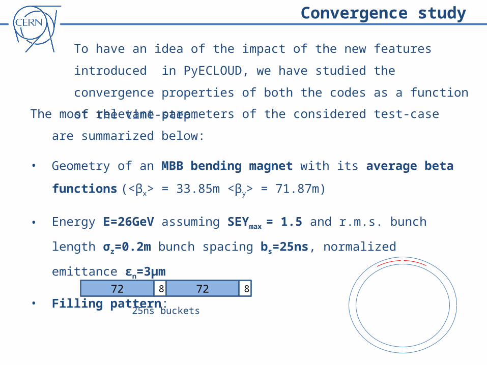
Convergence study
The most relevant parameters of the considered test-case are summarized below:
• Geometry of an MBB bending magnet with its average beta functions (<βx> =
33.85m <βy> = 71.87m)
• Energy E=26GeV assuming SEYmax = 1.5 and r.m.s. bunch length σz=0.2m bunch
spacing bs=25ns, normalized emittance εn=3μm
• Filling pattern:
To have an idea of the impact of the new features introduced in PyECLOUD, we
have studied the convergence properties of both the codes as a function of the
time-step.
72 8
25ns buckets
72 8
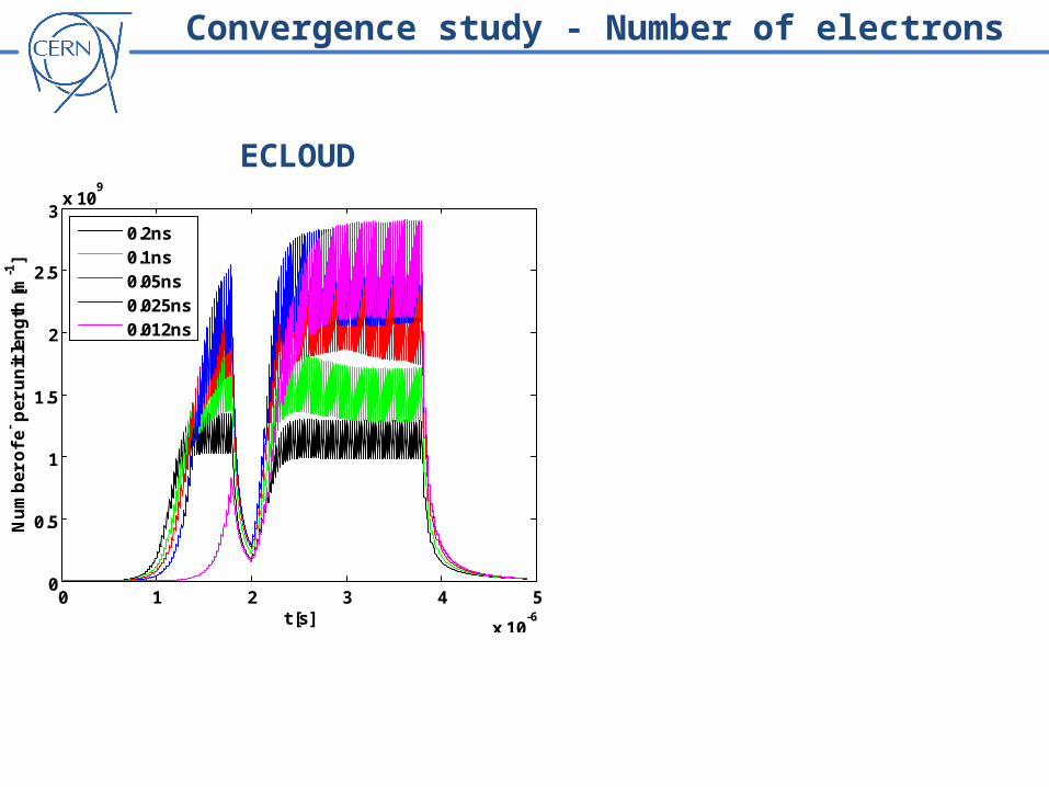
Convergence study - Number of electrons
0 1 2 3 4 5
x 10-6
0
0.5
1
1.5
2
2.5
3x 10
9
t [s]
Nu
mb
er
of
e- p
er
un
it le
ng
th [
m-1
]
0.2ns0.1ns0.05ns0.025ns0.012ns
ECLOUD
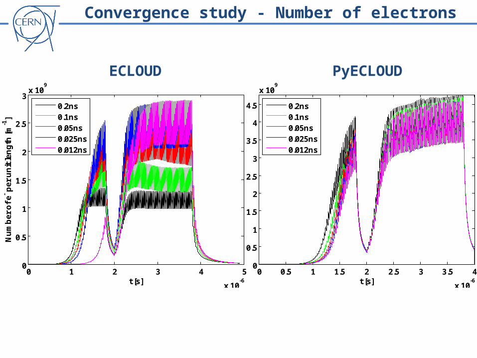
Convergence study - Number of electrons
0 0.5 1 1.5 2 2.5 3 3.5 4
x 10-6
0
0.5
1
1.5
2
2.5
3
3.5
4
4.5
x 109
t [s]
Nu
mb
er
of
e- p
er
un
it le
ng
th [
m-1
]
0.2ns0.1ns0.05ns0.025ns0.012ns
0 1 2 3 4 5
x 10-6
0
0.5
1
1.5
2
2.5
3x 10
9
t [s]
Nu
mb
er
of
e- p
er
un
it le
ng
th [
m-1
]
0.2ns0.1ns0.05ns0.025ns0.012ns
ECLOUD PyECLOUD
20 40 60 80 100 120 140 1600
0.5
1
1.5
2
2.5
3
3.5
4
4.5
Bunch passage
En
erg
y d
ep
os
itio
n [
W/m
]
0.2ns0.1ns0.05ns0.025ns0.012ns
20 40 60 80 100 120 140 160 180
0.5
1
1.5
2
2.5
3
3.5
Bunch passage
En
erg
y d
ep
os
itio
n [
W/m
]
0.2ns0.1ns0.05ns0.025ns
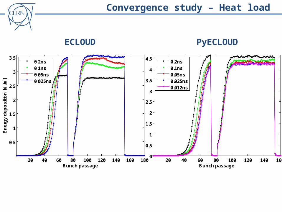
Convergence study – Heat load
ECLOUD PyECLOUD
0 0.5 1 1.5 2 2.5 3 3.5
x 10-6
0
2
4
6
8
10
12
14
16
18x 10
12
t [s]
e- d
en
sit
y a
t th
e c
en
ter
of
the
ch
am
be
r [m
-3]
0.2ns0.1ns0.05ns0.025ns0.012ns
0.5 1 1.5 2 2.5 3 3.5 4 4.5
x 10-6
0.5
1
1.5
2
2.5
3
x 1013
t [s]
e- d
en
sit
y a
t th
e c
en
ter
of
the
ch
am
be
r [m
-3]
0.2ns0.1ns0.05ns0.025ns
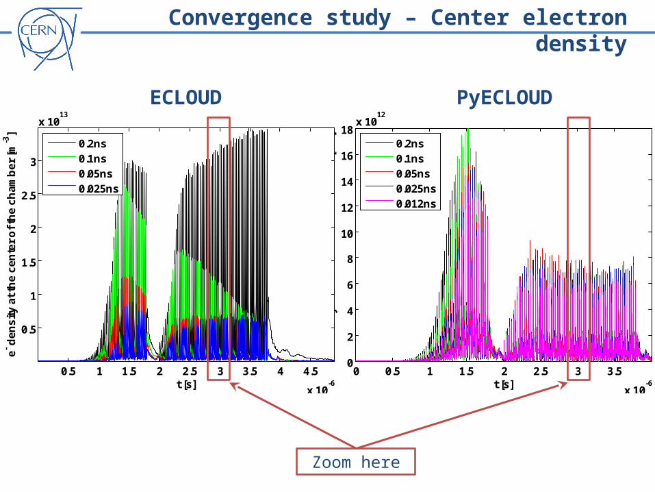
Convergence study – Center electron density
Zoom here
ECLOUD PyECLOUD
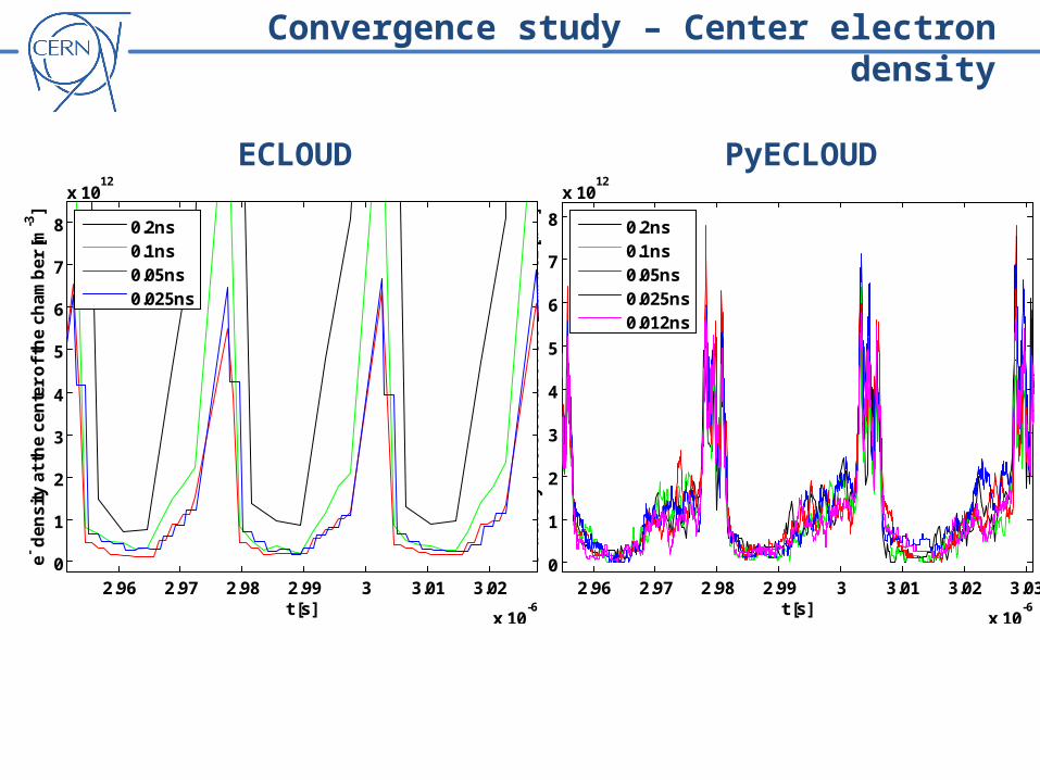
2.96 2.97 2.98 2.99 3 3.01 3.02 3.03
x 10-6
0
1
2
3
4
5
6
7
8
x 1012
t [s]
e- d
en
sit
y a
t th
e c
en
ter
of
the
ch
am
be
r [m
-3]
0.2ns0.1ns0.05ns0.025ns0.012ns
2.96 2.97 2.98 2.99 3 3.01 3.02
x 10-6
0
1
2
3
4
5
6
7
8
x 1012
t [s]
e- d
en
sit
y a
t th
e c
en
ter
of
the
ch
am
be
r [m
-3]
0.2ns0.1ns0.05ns0.025ns
Convergence study – Center electron density
ECLOUD PyECLOUD
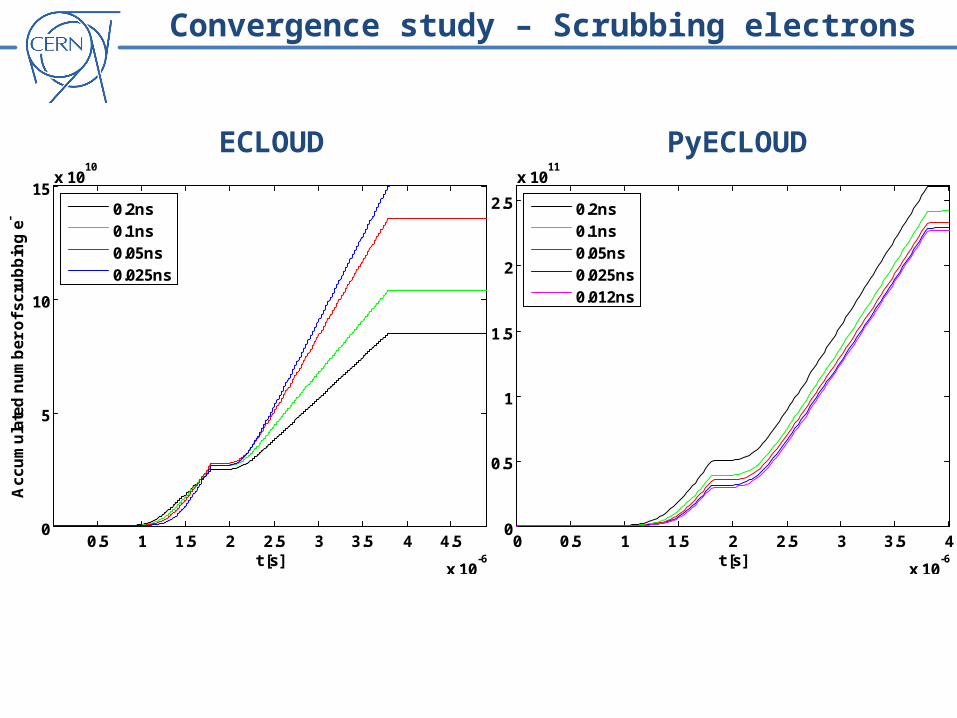
0 0.5 1 1.5 2 2.5 3 3.5 4
x 10-6
0
0.5
1
1.5
2
2.5
x 1011
t [s]
Ac
cu
mu
late
d n
um
be
r o
f s
cru
bb
ing
e-
0.2ns0.1ns0.05ns0.025ns0.012ns
0.5 1 1.5 2 2.5 3 3.5 4 4.5
x 10-6
0
5
10
15x 10
10
t [s]
Ac
cu
mu
late
d n
um
be
r o
f s
cru
bb
ing
e-
0.2ns0.1ns0.05ns0.025ns
Convergence study – Scrubbing electrons
ECLOUD PyECLOUD
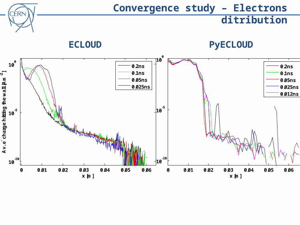
0 0.01 0.02 0.03 0.04 0.05 0.06
10-10
10-5
100
x [m]
Av
. e- c
ha
rge
hit
tin
g t
he
wa
ll [A
m-2
]
0.2ns0.1ns0.05ns0.025ns0.012ns
0 0.01 0.02 0.03 0.04 0.05 0.06
10-10
10-5
100
x [m]
Av
. e- c
ha
rge
hit
tin
g t
he
wa
ll [A
m-2
]
0.2ns0.1ns0.05ns0.025ns
Convergence study – Electrons ditribution
ECLOUD PyECLOUD
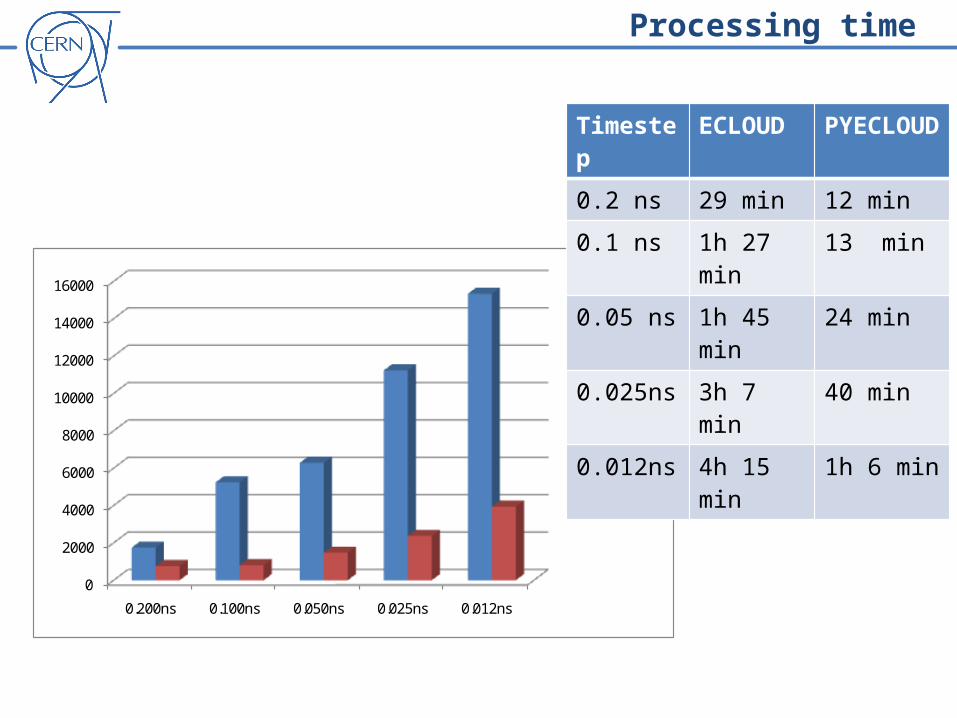
0
2000
4000
6000
8000
10000
12000
14000
16000
0.200ns 0.100ns 0.050ns 0.025ns 0.012ns
ECLOUD
PYECLOUD
Timestep ECLOUD PYECLOUD
0.2 ns 29 min 12 min
0.1 ns 1h 27 min 13 min
0.05 ns 1h 45 min 24 min
0.025ns 3h 7 min 40 min
0.012ns 4h 15 min 1h 6 min
Processing time
Outline
• Why a new code for electron cloud build-up simulation?
• From ECLOUD to PyECLOUD
o Management of macroparticle size and number
o back-tracking algorithm for the impacting electrons
o Beam field calculation
o Space charge field
• Preliminary convergence study
• PyECLOUD at work
• Conclusion and future work
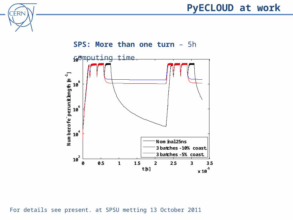
PyECLOUD at work
0 0.5 1 1.5 2 2.5 3 3.5
x 10-5
102
104
106
108
1010
t [s]
Nu
mb
er
of e
- per
un
it le
ng
th [m
-1]
Nominal 25ns3 batches - 10% coast.3 batches - 5% coast.
SPS: More than one turn – 5h computing time
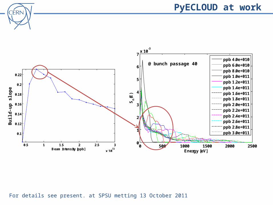
For details see present. at SPSU metting 13 October 2011
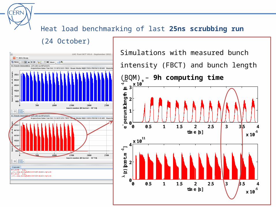
Heat load benchmarking of last 25ns scrubbing run (24 October)
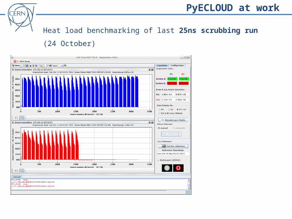
PyECLOUD at work
Heat load benchmarking of last 25ns scrubbing run (24 October)
0 0.5 1 1.5 2 2.5 3 3.5 4
x 10-5
0
1
2
3x 10
9
time [s]
e- p
er
un
it le
ng
th [
m-1
]
0 0.5 1 1.5 2 2.5 3 3.5 4
x 10-5
0
2
4x 10
11
time [s]
(z
) [p
rot.
m-1
]
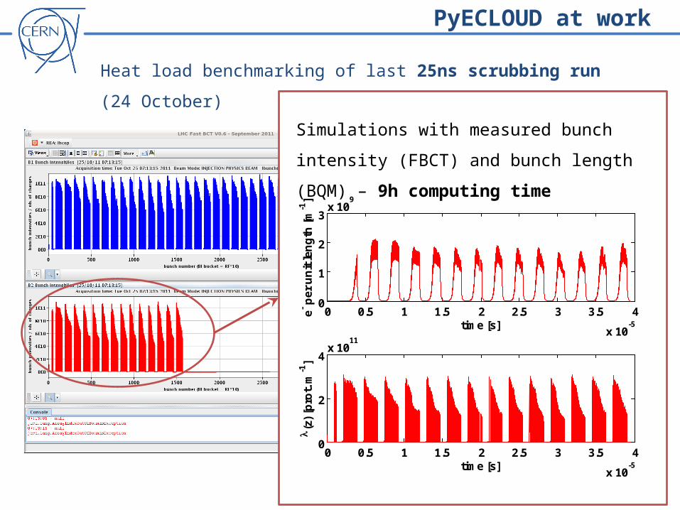
Simulations with measured bunch intensity (FBCT)
and bunch length (BQM) – 9h computing time
PyECLOUD at work
Heat load benchmarking of last 25ns scrubbing run (24 October)
0 0.5 1 1.5 2 2.5 3 3.5 4
x 10-5
0
1
2
3x 10
9
time [s]
e- p
er
un
it le
ng
th [
m-1
]
0 0.5 1 1.5 2 2.5 3 3.5 4
x 10-5
0
2
4x 10
11
time [s]
(z
) [p
rot.
m-1
]
Simulations with measured bunch intensity (FBCT)
and bunch length (BQM) – 9h computing time
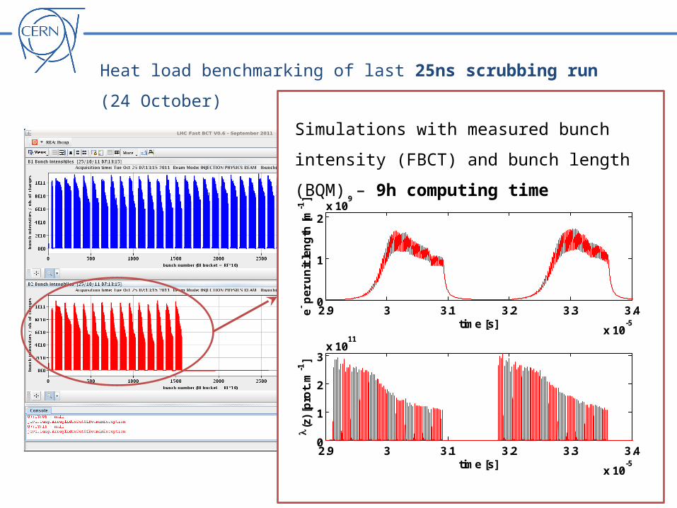
Heat load benchmarking of last 25ns scrubbing run (24 October)
2.9 3 3.1 3.2 3.3 3.4
x 10-5
0
1
2x 10
9
time [s]
e- p
er
un
it le
ng
th [
m-1
]
2.9 3 3.1 3.2 3.3 3.4
x 10-5
0
1
2
3x 10
11
time [s]
(z
) [p
rot.
m-1
]
Simulations with measured bunch intensity (FBCT)
and bunch length (BQM) – 9h computing time
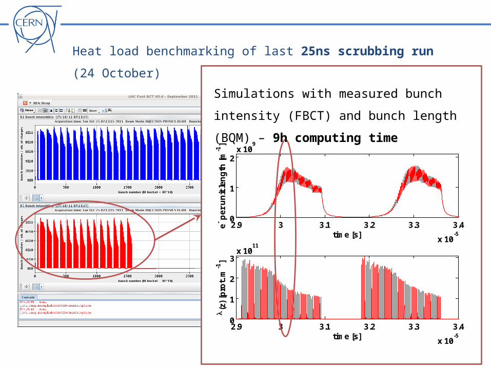
Heat load benchmarking of last 25ns scrubbing run (24 October)
2.9 3 3.1 3.2 3.3 3.4
x 10-5
0
1
2x 10
9
time [s]
e- p
er
un
it le
ng
th [
m-1
]
2.9 3 3.1 3.2 3.3 3.4
x 10-5
0
1
2
3x 10
11
time [s]
(z
) [p
rot.
m-1
]
Simulations with measured bunch intensity (FBCT)
and bunch length (BQM) – 9h computing time
3 3.002 3.004 3.006 3.008 3.01 3.012 3.014 3.016
x 10-5
0
1
2x 10
9
time [s]
e- p
er
un
it le
ng
th [
m-1
]
3 3.002 3.004 3.006 3.008 3.01 3.012 3.014 3.016
x 10-5
0
1
2
3x 10
11
time [s]
(z
) [p
rot.
m-1
]
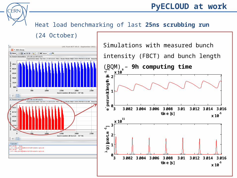
Heat load benchmarking of last 25ns scrubbing run (24 October)
Simulations with measured bunch intensity (FBCT)
and bunch length (BQM) – 9h computing time
PyECLOUD at work
For details see present. at SPSU metting 13 October 2011
0 500 1000 1500 2000 25000
1
2
3
4
5
6
7x 10
-3
Energy [eV]
Sn(E
)
ppb 4.0e+010ppb 6.0e+010ppb 8.0e+010ppb 1.0e+011ppb 1.2e+011ppb 1.4e+011ppb 1.6e+011ppb 1.8e+011ppb 2.0e+011ppb 2.2e+011ppb 2.4e+011ppb 2.6e+011ppb 2.8e+011ppb 3.0e+011
0.5 1 1.5 2 2.5 3
x 1011
0.1
0.12
0.14
0.16
0.18
0.2
0.22
n
Beam intensity [ppb]
Build
-up
slop
e
@ bunch passage 40
PyECLOUD at work
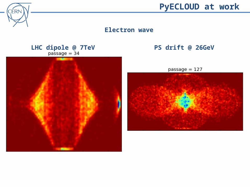
Electron wave
LHC dipole @ 7TeV PS drift @ 26GeV
PyECLOUD at work
Outline
• Why a new code for electron cloud build-up simulation?
• From ECLOUD to PyECLOUD
o Management of macroparticle size and number
o Back-tracking algorithm for the impacting electrons
o Beam field calculation
o Space charge field
• Preliminary convergence study
• PyECLOUD at work
• Conclusion and future work
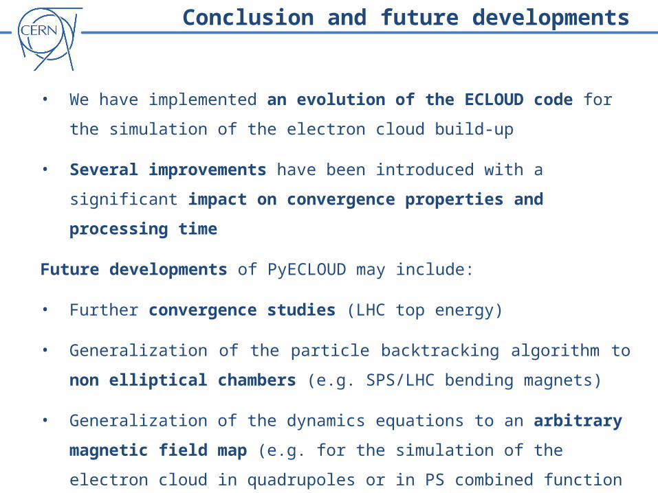
Conclusion and future developments
• We have implemented an evolution of the ECLOUD code for the simulation of the
electron cloud build-up
• Several improvements have been introduced with a significant impact on
convergence properties and processing time
Future developments of PyECLOUD may include:
• Further convergence studies (LHC top energy)
• Generalization of the particle backtracking algorithm to non elliptical chambers
(e.g. SPS/LHC bending magnets)
• Generalization of the dynamics equations to an arbitrary magnetic field map (e.g.
for the simulation of the electron cloud in quadrupoles or in PS combined function
magnets)

Thanks for your attention!
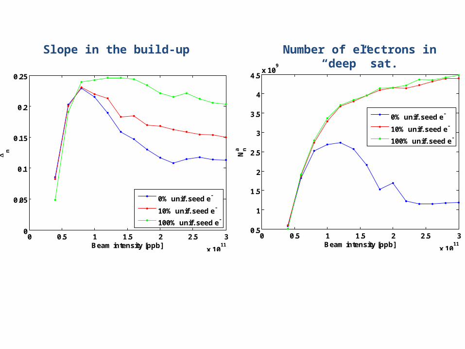
Slope in the build-up
0 0.5 1 1.5 2 2.5 3
x 1011
0
0.05
0.1
0.15
0.2
0.25
n
Beam intensity [ppb]
0% unif. seed e-
10% unif. seed e-
100% unif. seed e-
0 0.5 1 1.5 2 2.5 3
x 1011
0.5
1
1.5
2
2.5
3
3.5
4
4.5x 10
9
Na n
Beam intensity [ppb]
0% unif. seed e-
10% unif. seed e-
100% unif. seed e-
Number of electrons in “deep” sat.
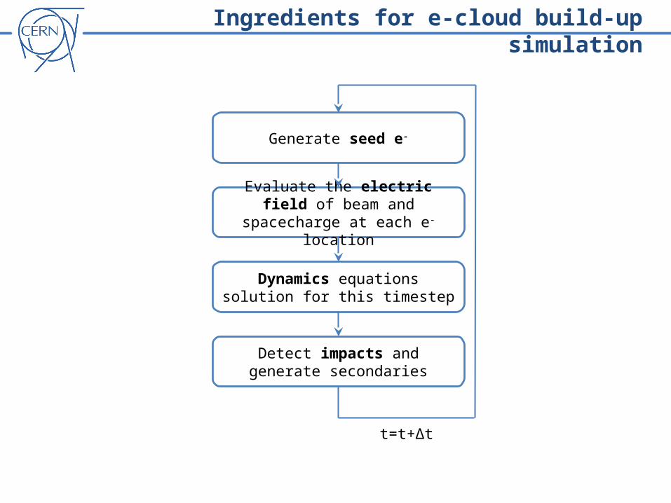
t=t+Δt
Evaluate the electric field of beam and spacecharge at each e- location
Generate seed e-
Dynamics equations solution for this timestep
Detect impacts and generate secondaries
Ingredients for e-cloud build-up simulation
Recommended