1
Prediction of Transmission Distortion for
Wireless Video Communication: Part I:
AnalysisZhifeng Chen and Dapeng Wu
Department of Electrical and Computer Engineering, University of Florida, Gainesville, Florida
32611
Abstract
In the wireless video communication system, transmission distortion, caused by packet transmission
errors, is a non-linear time-variant function of video frame statistics, channel condition and system
parameters. By modeling the transmission distortion process as output of the random video sequence
and channel error processes, the system can be modeled as an equivalent non-linear time-variant system.
In this paper, for the first time, we identify the governing law that describes how the transmission
distortion process evolves over time, and analytically derive it as a closed-form function of frame statistics,
channel condition, and system parameters through a divide-and-conquer approach. Besides deriving
the transmission distortion formula, this paper also identifies two important properties of transmission
distortion for the first time. The first property is that the clipping noise, produced by non-linear clipping,
causes decay of propagated error. The second property is that the correlation between motion vector
concealment error and propagated error is negative, and has dominant impact on transmission distortion
among all other correlations. In this paper, we also identify the relationship between our result and
existing models, and specify the conditions, under which those models are accurate.
Index Terms
Wireless video, transmission distortion, clipping noise, slice data partitioning, Unequal Error Protec-
tion (UEP), time-varing channel.
Please direct all correspondence to Prof. Dapeng Wu, University of Florida, Dept. of Electrical & Computer Engineering,
P.O.Box 116130, Gainesville, FL 32611, USA. Tel. (352) 392-4954. Fax (352) 392-0044. Email: [email protected]. Homepage:
http://www.wu.ece.ufl.edu.
August 11, 2010 DRAFT

2
I. INTRODUCTION
Both multimedia technology and mobile communications have experienced massive growth and com-
mercial success in recent years. As the two technologies converge, wireless video, such as video phone
and mobile TV in 3G/4G systems, is expected to achieve unprecedented growth and worldwide success.
However, different from the traditional video coding system, transmitting video over wireless with good
quality or low end-to-end distortion is particularly challenging since the received video is subject to not
only quantization error but also transmission error. In a wireless video communication system, end-to-end
distortion consists of two parts: quantization distortion and transmission distortion. Quantization distortion
is caused by quantization errors during the encoding process, and has been extensively studied in rate
distortion theory [1], [2]. Transmission distortion is caused by packet errors during the transmission of
a video sequence, and it is the major part of the end-to-end distortion in delay-sensitive wireless video
communication1 under high packet error probability (PEP), e.g., in a wireless fading channel.
The capability of predicting transmission distortion at the transmitter can assist in designing video
encoding and transmission schemes that achieve maximum video quality under resource constraints.
Specifically, transmission distortion prediction can be used in the following three applications in video
encoding and transmission: 1) mode selection, which is to find the best intra/inter-prediction mode for
encoding a macroblock (MB) with the minimum rate-distortion (R-D) cost given the instantaneous PEP,
2) cross-layer encoding rate control, which is to control the instantaneously encoded bit rate for a real-
time encoder to minimize the frame-level end-to-end distortion given the instantaneous PEP, e.g., in
video conferencing, 3) packet scheduling, which chooses a subset of packets of the pre-coded video to
transmit and intentionally discards the remaining packets to minimize the GOP-level (Group of Picture)
end-to-end distortion given the average PEP and average burst length, e.g., in streaming pre-coded video
over networks. All the three applications require a formula for predicting how transmission distortion
is affected by their respective control policy, in order to choose the optimal mode or encoding rate or
transmission schedule.
However, predicting transmission distortion poses a great challenge due to the spatio-temporal corre-
lation inside the input video sequence, the nonlinearity of both the encoder and the decoder, and varying
PEP in time-varying channels. In a typical video codec, the temporal correlation among consecutive
frames and the spatial correlation among the adjacent pixels of one frame are exploited to improve the
1Delay-sensitive wireless video communication usually does not allow retransmission to correct packet errors since
retransmission may cause long delay.
August 11, 2010 DRAFT

3
coding efficiency. Nevertheless, such a coding scheme brings much difficulty in predicting transmission
distortion because a packet error will degrade not only the video quality of the current frame but also the
following frames due to error propagation. In addition, as we will see in Section IV, the nonlinearity of
both the encoder and the decoder makes the instantaneous transmission distortion not equal to the sum
of distortions caused by individual error events. Furthermore, in a wireless fading channel, the PEP is
time-varying, which makes the error process a non-stationary random process and hence, as a function
of the error process, the distortion process is also a non-stationary random process.
In this paper, we derived the transmission distortion formulae for wireless video communication
systems. With consideration of spatio-temporal correlation, nonlinear codec and time-varying channel,
our distortion prediction formulae provide, for the first time, the following capabilities: 1) support of
prediction at different levels (e.g., pixel/frame/GOP level), 2) support of prediction for multi-reference
motion compensation, 3) support of prediction under slice data partitioning, 4) support of prediction
under arbitrary slice-level packetization with Flexible Macroblock Ordering (FMO) mechanism, 5) being
applicable to time-varying channels, 6) one unified formula for both I-MB and P-MB, and 7) support
of prediction for both low motion and high motion video sequences. Besides deriving the transmission
distortion formulae, this paper also identified two important properties of transmission distortion for the
first time: 1) clipping noise, produced by non-linear clipping, causes decay of propagated error; 2) the
correlation between motion vector concealment error and propagated error is negative, and has dominant
impact on transmission distortion, among all the correlations between any two of the four components
in transmission error. We also discussed the relationship between our formula and existing models.
The rest of the paper is organized as follows. Section II reviews existing works for estimating distortion
caused by packet transmission error. Section III presents the preliminaries of our system model under
study to facilitate the derivations in the later sections, and illustrates the limitations of existing transmission
distortion models. In Section IV, we derive the transmission distortion formula as a function of frame
statistics, channel condition, and system parameters. Section V discusses the relationship between our
formula and the existing models. In Section VI, we extend formulae for PTD and FTD from single-
reference to multi-reference. Section VII concludes the paper.
II. RELATED WORKS
According to the aforementioned three applications, the existing algorithms for estimating transmission
distortion can be categorized into the following three classes: 1) pixel-level or block-level algorithms
(applied to mode selection), e.g., Recursive Optimal Per-pixel Estimate (ROPE) algorithm [3] and Law
August 11, 2010 DRAFT

4
of Large Number (LLN) algorithm [4], [5]; 2) frame-level or packet-level or slice-level algorithms
(applied to cross-layer encoding rate control) [6], [7], [8], [9]; 3) GOP-level or sequence-level algorithms
(applied to packet scheduling) [10], [11], [12], [13], [14]. Although the existing distortion estimation
algorithms work at different levels, they share some common properties, which come from the inherent
characteristics of wireless video communication system, that is, spatio-temporal correlation, nonlinear
codec and time-varying channel. In this paper, we use the divide-and-conquer approach to decompose
complicated transmission distortion into four components, and analyze their effects on transmission
distortion individually. This divide-and-conquer approach enables us to identify the governing law that
describes how the transmission distortion process evolves over time.
Stuhlmuller et al. [6] observed that the distortion caused by the propagated error decays over time due to
spatial filtering and intra coding of MBs, and analytically derived a formula for estimating transmission
distortion under spatial filtering and intra coding. The effect of spatial filtering is analyzed under the
implicit assumption that MVs are always correctly received at the receiver, while the effect of intra
coding is modeled as a linear decay under another implicit assumption that the I-MBs are also always
correctly received at the receiver. However, these two assumptions are usually not valid in realistic delay-
sensitive wireless video communication. To address this, this paper derives the transmission distortion
formula under the condition that both I-MBs and MVs may be erroneous at the receiver. In addition,
we observe an interesting phenomenon that even without using the spatial filtering and intra coding, the
distortion caused by the propagated error still decays! We identify, for the first time, that this decay is
caused by non-linear clipping, which is used to clip those out-of-range2 reconstructed pixel after motion
compensation; this is the first of the two properties identified in this paper. While such out-of-range
values produced by the inverse transform of quantized transform coefficients is negligible at the encoder,
its counterpart produced by transmission error at the decoder has significant impact on transmission
distortion.
Some existing works [6], [7] estimate transmission distortion based on a linear time-invariant (LTI)
system model, which regards packet error as input and transmission distortion as output. The LTI model
simplifies the analysis of transmission distortion. However, it sacrifices accuracy in distortion estimation
since it neglects the effect of correlation between newly induced error and propagated error. Liang
et al. [14] studied the effect of correlation and observed that the LTI models [6], [7] underestimate
transmission distortion due to the positive correlation between two adjacent erroneous frames; however,
2A reconstructed pixel value may be out of the range of the original pixel value, e.g., [0, 255].
August 11, 2010 DRAFT

5
they did not consider the effect of motion vector (MV) error on transmission distortion and their algorithm
was not tested with high motion videos. To address these issues and find the cause of the under-estimation,
this paper classifies the transmission reconstructed error into three individual random errors, namely,
Residual Concealment Error (RCE), MV Concealment Error (MVCE), and propagated error; the first two
types of error are called newly induced error. We identify, for the first time, that MVCE is negatively
correlated with propagated error and this correlation has dominant impact on transmission distortion,
among all the correlations between any two of the three error types, for high motion videos; this is the
second of the two properties identified in this paper. For this reason, as long as MV transmission errors
exist in high motion videos, the LTI model over-estimates transmission distortion. We also quantifies the
effect of individual error types and their correlations on transmission distortion in this paper. Thanks
to the analysis of correlation effect, our distortion formula is accurate for both low motion video and
high motion video as verified by experimental results. Another merit of considering the effect of MV
error on transmission distortion is the applicability of our results to video communication with slice data
partitioning, where the residual and MV could be transmitted under Unequal Error Protection (UEP).
Refs. [3], [4], [8], [9] proposed some models to estimate transmission distortion under the consideration
that both MV and I-MB may experience transmission errors. However, the parameters in the linear
models [8], [9] can only be acquired by experimentally curve-fitting over multiple frames, which forbids
the models from estimating instantaneous distortion. In addition, the linear models [8], [9] still assume
there is no correlation between the newly induced error and propagated error. In Ref. [3], the ROPE
algorithm considers the correlation between MV concealment error and propagated error by recursively
calculating the second moment of the reconstructed pixel value. However, ROPE neglects the non-
linear clipping function and therefore over-estimates the distortion. In addition, the extension of ROPE
algorithm [15] to support the averaging operations, such as interpolation and deblocking filtering in
H.264, requires intensive computation of correlation coefficients due to the high correlation between
reconstructed values of adjacent pixels, and thereby prohibiting it from applying to H.264. In H.264
reference code JM14.0 [16], the LLN algorithm [4] is adopted since it is capable of supporting both
clipping and averaging operations. However, in order to predict transmission distortion, all possible error
events for each pixel in all frames should be simulated at the encoder, which significantly increases the
complexity of the encoder. Different from Refs. [3], [4], the divide-and-conquer approach in this paper
enables our formula to provide not only more accurate prediction but also lower complexity and higher
degree of extensibility. The multiple reference picture motion compensated prediction extended from the
single reference is analyzed in Section VI, and, for the first time, the effect of multiple references on
August 11, 2010 DRAFT

6
transmission distortion is quantified. In addition, the transmission distortion formula derived in this paper
is unified for both I-MBs and P-MBs, in contrast to two different formulae in Refs. [3], [8], [9].
Different from wired channels, wireless channels suffer from multipath fading, which can be regarded
as multiplicative random noise. Fading leads to time-varying PEP and burst errors in wireless video
communication. Ref. [6] uses a two-state stationary Markov chain to model burst errors. However, even
if the channel gain is stationary, packet error process is a non-stationary random process. Specifically,
since PEP is a function of the channel gain [17], which is not constant in a wireless fading channel,
instantaneous PEP is also not constant. This means the probability distribution of packet error state
is time-varying in wireless fading channels, that is, the packet error process is a non-stationary random
process. Hence the Markov chain in Ref. [6] is neither stationary, nor ergodic for wireless fading channel.
As a result, averaging the burst length and PEP as in Ref. [6] cannot accurately predict instantaneous
distortion. To address this, this paper derives the formula for Pixel-level Transmission Distortion (PTD) by
considering non-stationarity over time. Regarding the Frame-level Transmission Distortion (FTD), since
two adjacent MBs may be assigned to two different packets, under the slice-level packetization and FMO
mechanism in H.264 [18], [19], their error probability could be different. However, existing frame-level
distortion models [6], [7], [8], [9] assume all pixels in the same frame experience the same channel
condition. As a result, the applicable scope of those models are limited to video with small resolution.
In contrast, this paper derives the formula for FTD by considering non-stationarity over space. Due to
consideration of non-stationarity over time and over space, our formula provides an accurate prediction
of transmission distortion in a time-varying channel.
III. SYSTEM DESCRIPTION
A. Structure of a Wireless Video Communication System
Fig. 1 shows the structure of a typical wireless video communication system. It consists of an encoder,
two channels and a decoder where residual packets and MV packets are transmitted over their respective
channels. If residual packets or MV packets are erroneous, the error concealment module will be activated.
In typical video encoders such as H.263/264 and MPEG-2/4 encoders, the functional blocks can be divided
into two classes: 1) basic parts, such as predictive coding, transform, quantization, entropy coding, motion
compensation, and clipping; and 2) performance-enhanced parts, such as interpolation filtering, deblocking
filtering, B-frame, multi-reference prediction, etc. Although the up-to-date video encoder includes more
and more performance-enhanced parts, the basic parts do not change. In this paper, we use the structure
in Fig. 1 for transmission distortion analysis.
August 11, 2010 DRAFT
7
Videocapture
Input
T/Q-Q-1/T-1
ResidualChannel
+
Motioncompensation
Memory
Motionestimation
MVChannel
Q-1/T-1
+
Motioncompensation
MV Errorconcealment
ChannelEncoder Decoder
Videodisplay
Output
Clipping Clipping
Memory
keu
kuvm
(
keuˆ
kfu1ˆ −kfu
1ˆ −+k
kfumvu
1~
~ −+k
kfuvmu
keu~
kfu
~
1~ −kfu
Residual ErrorConcealment
keuˆ
keu(
kfu
kumv
S(r)
S(m)
‘0’
‘0’
‘1’
‘1’
Fig. 1. System structure, where T, Q, Q−1, and T−1 denote transform, quantization, inverse quantization, and inverse transform,
respectively.
Note that in this system, both residual channel and MV channel are application-layer channels; specif-
ically, both channels consist of entropy coding and entropy decoding, networking layers3, and physical
layer (including channel encoding, modulation, wireless fading channel, demodulation, channel decoding).
Although the residual channel and MV channel usually share the same physical-layer channel, the two
application-layer channels may have different parameter settings (e.g., different channel code-rate) for
the slice data partitioning under UEP. For this reason, our formula obtained from the structure in Fig. 1
can be used to estimate transmission distortion for an encoder with slice data partitioning.
B. Clipping Noise
In this subsection, we examine the effect of clipping noise on the reconstruction pixel value along
each pixel trajectory over time (frames). All pixel positions in a video sequence form a three-dimensional
spatio-temporal domain, i.e., two dimensions in spatial domain and one dimension in temporal domain.
Each pixel can be uniquely represented by uk in this three-dimensional time-space, where k means the
k-th frame in temporal domain and u is a two-dimensional vector in spatial domain. The philosophy
3Here, networking layers can include any layers other than physical layer.
August 11, 2010 DRAFT

8
behind inter-coding of a video sequence is to represent the video sequence by virtual motion of each
pixel, i.e., each pixel recursively moves from position vk−1 to position uk. The difference between these
two positions is a two-dimensional vector called MV of pixel uk, i.e., mvku = vk−1−uk. The difference
between the pixel values of these two positions is called residual of pixel uk, that is, eku = fk
u− fk−1u+mvk
u
4.
Recursively, each pixel in the k-th frame has one and only one reference pixel trajectory backward towards
the latest I-frame.
At the encoder, after transform, quantization, inverse quantization, and inverse transform for the
residual, the reconstructed pixel value for uk may be out-of-range and should be clipped as
fku = Γ(fk−1
u+mvku
+ eku), (1)
where Γ(·) function is a clipping function defined by
Γ(x) =
γL, x < γL
x, γL ≤ x ≤ γH
γH , x > γH ,
(2)
where γL and γH are user-specified low threshold and high threshold, respectively. Usually, γL = 0 and
γH = 255.
The residual and MV at the decoder may be different from their counterparts at the encoder because
of channel impairments. Denote mvku and ek
u the MV and residual at the decoder, respectively. Then, the
reference pixel position for uk at the decoder is vk−1 = uk + mvku, and the reconstructed pixel value
for uk at the decoder is
fku = Γ(fk−1
u+gmvku
+ eku). (3)
In error-free channels, the reconstructed pixel value at the receiver is exactly the same as the recon-
structed pixel value at the transmitter, because there is no transmission error and hence no transmission
distortion. However, in error-prone channels, we know from (3) that fku is a function of three factors: the
received residual eku, the received MV mvk
u, and the propagated error fk−1u+gmvk
u
. The received residual eku
depends on three factors, namely, 1) the transmitted residual eku, 2) the residual packet error state, which
depends on instantaneous residual channel condition, and 3) the residual error concealment algorithm if
the received residual packet is erroneous. Similarly, the received MV mvku depends on 1) the transmitted
mvku, 2) the MV packet error state, which depends on instantaneous MV channel condition, and 3) the
4For simplicity of notation, we move the superscript k of u to the superscript k of f whenever u is the subscript of f .
August 11, 2010 DRAFT
9
TABLE I
NOTATIONS
uk : Three-dimensional vector that denotes a pixel position in an video sequence
fku : Value of the pixel uk
eku : Residual of the pixel uk
mvku : MV of the pixel uk
∆ku : Clipping noise of the pixel uk
εku : Residual concealment error of the pixel uk
ξku : MV concealment error of the pixel uk
ζku : Transmission reconstructed error of the pixel uk
Sku : Error state of the pixel uk
P ku : Error probability of the pixel uk
Dku : Transmission distortion of the pixel uk
Dk : Transmission distortion of the k-th frame
Vk : Set of all the pixels in the k-th frame
|V| : Number of elements in set V (cardinality of V)
αk : Propagation factor of the k-th frame
βk : Percentage of I-MBs in the k-th frame
λk : Correlation ratio of the k-th frame
wk(j): pixel percentage of using frame k − j as reference in the k-th frame
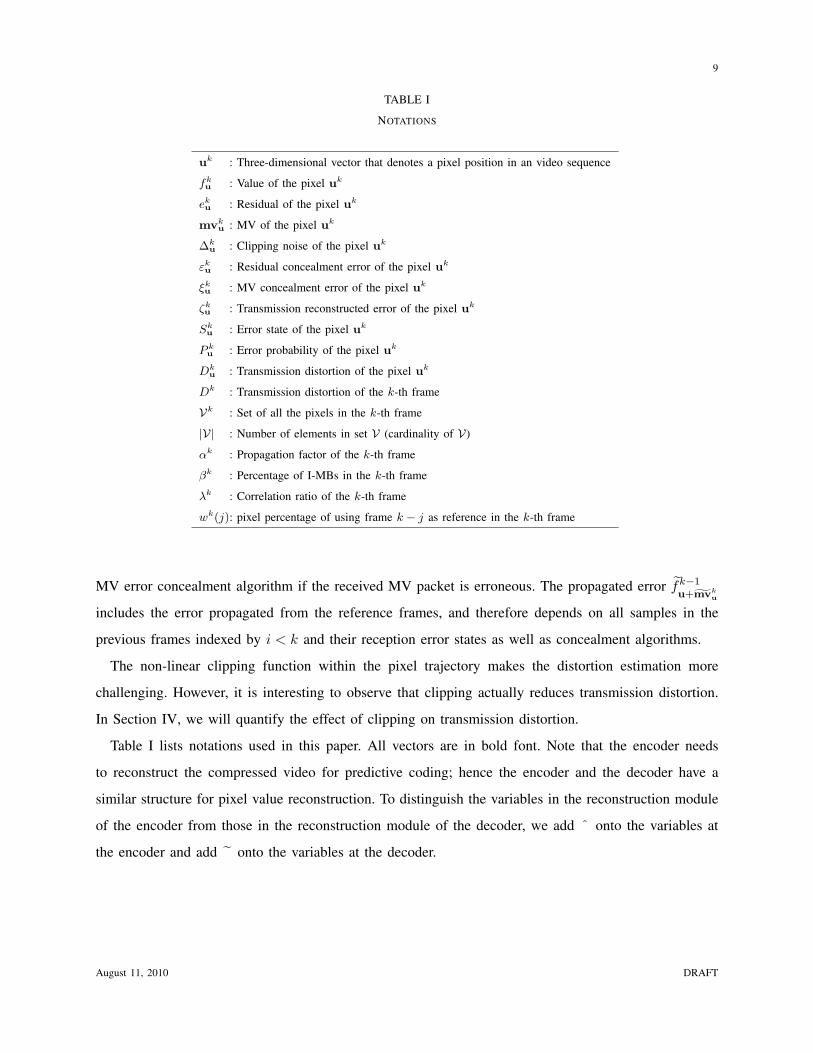
MV error concealment algorithm if the received MV packet is erroneous. The propagated error fk−1u+gmvk
u
includes the error propagated from the reference frames, and therefore depends on all samples in the
previous frames indexed by i < k and their reception error states as well as concealment algorithms.
The non-linear clipping function within the pixel trajectory makes the distortion estimation more
challenging. However, it is interesting to observe that clipping actually reduces transmission distortion.
In Section IV, we will quantify the effect of clipping on transmission distortion.
Table I lists notations used in this paper. All vectors are in bold font. Note that the encoder needs
to reconstruct the compressed video for predictive coding; hence the encoder and the decoder have a
similar structure for pixel value reconstruction. To distinguish the variables in the reconstruction module
of the encoder from those in the reconstruction module of the decoder, we add ˆ onto the variables at
the encoder and add ˜ onto the variables at the decoder.
August 11, 2010 DRAFT

10
C. Definition of Transmission Distortion
In this subsection, we define PTD and FTD to be derived in Section IV. To calculate FTD, we need
some notations from set theory. In a video sequence, all pixel positions in the k-th frame form a two-
dimensional vector set Vk, and we denote the number of elements in set Vk by |Vk|. So, for any pixel
at position u in the k-th frame, i.e., u ∈ Vk, its reference pixel position is chosen from set Vk−1 for
single-reference.
For a transmitter with feedback acknowledgement of whether a packet is correctly received at the
receiver (called acknowledgement feedback), fku at the decoder side can be perfectly reconstructed by
the transmitter, as long as the transmitter knows the error concealment algorithm used by the receiver.
Then, the transmission distortion for the k-th frame can be calculated by mean squared error (MSE) as
MSEk =1|Vk| ·
∑
u∈Vk
[(fku − fk
u)2]. (4)
For the encoder, every pixel intensity fku of the random input video sequence is a random variable. For
any encoder with hybrid coding (see Fig. 1), the residual eku, MV mvk
u, and reconstructed pixel value fku
are functions of fku; so they are also random variables before motion estimation5. Given the Probability
Mass Function (PMF) of fku and fk
u , we define the transmission distortion for pixel uk or PTD by
Dku , E[(fk
u − fku)2], (5)
and we define the transmission distortion for the k-th frame or FTD by
Dk , E[1|Vk| ·
∑
u∈Vk
(fku − fk
u)2]. (6)
It is easy to prove that the relationship between FTD and PTD is characterized by
Dk =1|Vk| ·
∑
u∈Vk
Dku. (7)
If the number of bits used to compress a frame is too large to be contained in one packet, the bits of the
frame are split into multiple packets. In a time-varying channel, different packet of the same frame may
experience different packet error probability (PEP). If pixel uk and pixel vk belong to different packets,
the PMF of fku may be different from the PMF of fk
v even if fku and fk
v are identically distributed. In other
words, Dku may be different from Dk
v even if pixel uk and pixel vk are in the neighboring MBs when
5In applications such as cross-layer encoding rate control, distortion estimation for rate-distortion optimized bit allocation is
required before motion estimation.
August 11, 2010 DRAFT

11
FMO is activated. As a result, FTD Dk in (7) may be different from PTD Dku in (5). For this reason, we
will derive formulae for both PTD and FTD, respectively. Note that most existing frame-level distortion
models [6], [7], [8], [9] assume that all pixels in the same frame experience the same channel condition
and simply use (5) for FTD; however this assumption is not valid for high-resolution/high-quality video
transmission over a time-varying channel.
In fact, (7) is a general form for distortions of all levels. If |V| = 1, (7) reduces to (5). For slice/packet-
level distortion, V is the set of the pixels contained in a slice/packet. For GOP-level distortion, V is the
set of the pixels contained in a GOP. In this paper, we only show how to derive formulae for PTD and
FTD. Our methodology is also applicable to deriving formulae for slice/packet/GOP-level distortion by
using appropriate V .
D. Limitations of the Existing Transmission Distortion Models
In this subsection, we show that clipping noise has significant impact on transmission distortion, and
neglect of clipping noise in existing models results in inaccurate estimation of transmission distortion.
We define the clipping noise for pixel uk at the encoder as
∆ku , (fk−1
u+mvku
+ eku)− Γ(fk−1
u+mvku
+ eku), (8)
and the clipping noise for pixel uk at the decoder as
∆ku , (fk−1
u+gmvku
+ eku)− Γ(fk−1
u+gmvku
+ eku). (9)
Using (1), Eq. (8) becomes
fku = fk−1
u+mvku
+ eku − ∆k
u, (10)
and using (3), Eq. (9) becomes
fku = fk−1
u+gmvku
+ eku − ∆k
u, (11)
where ∆ku only depends on the video content and encoder structure, e.g., motion estimation, quantization,
mode decision and clipping function; and ∆ku depends on not only the video content and encoder structure,
but also channel conditions and decoder structure, e.g., error concealment and clipping function.
In most existing works, both ∆ku and ∆k
u are neglected, i.e., these works assume fku = fk−1
u+mvku+ek
u and
fku = fk−1
u+gmvku
+ eku. However, this assumption is only valid for stored video or error-free communication.
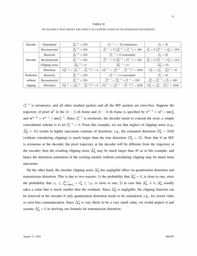
For error-prone communication, decoder clipping noise ∆ku has a significant impact on transmission
distortion and hence should not be neglected. To illustrate this, Table II shows an example for the system
in Fig. 1, where only the residual packet in the (k − 1)-th frame is erroneous at the decoder (i.e.,
August 11, 2010 DRAFT
12
TABLE II
AN EXAMPLE THAT SHOWS THE EFFECT OF CLIPPING NOISE ON TRANSMISSION DISTORTION.
Encoder Transmitted fk−2w = 250 ek−1
v = −50 (erroneous) eku = 50
Reconstructed fk−2w = 250 fk−1
v = Γ(fk−2w + ek−1
v ) = 200 fku = Γ(fk−1
v + eku) = 250
Received efk−2w = 250 eek−1
v = 0 (concealed) eeku = 50
Decoder Reconstructed efk−2w = 250 efk−1
v = Γ( efk−2w + eek−1
v ) = 250 efku = Γ( efk−1
v + eeku) = 255
Clipping noise e∆k−2w = 0 e∆k−1
v = 0 e∆ku = 45
Distortion Dk−2w = (fk−2
w − efk−2w )2 = 0 Dk−1
v = (fk−1v − efk−1
v )2 = 2500 Dku = (fk
u − efku)2 = 25
Prediction Received efk−2w = 250 eek−1
v = 0 (concealed) eeku = 50
without Reconstructed efk−2w = 250 efk−1
v = efk−2w + eek−1
v = 250 efku = efk−1
v + eeku = 300
clipping Distortion Dk−2w = (fk−2
w − efk−2w )2 = 0 Dk−1
v = (fk−1v − efk−1
v )2 = 2500 Dku = (fk
u − efku)2 = 2500
ek−1v is erroneous), and all other residual packets and all the MV packets are error-free. Suppose the
trajectory of pixel uk in the (k − 1)-th frame and (k − 2)-th frame is specified by vk−1 = uk + mvku
and wk−2 = vk−1 + mvk−1v . Since ek−1
v is erroneous, the decoder needs to conceal the error; a simple
concealment scheme is to let ek−1v = 0. From this example, we see that neglect of clipping noise (e.g.,
∆ku = 45) results in highly inaccurate estimate of distortion, e.g., the estimated distortion Dk
u = 2500
(without considering clipping) is much larger than the true distortion Dku = 25. Note that if an MV
is erroneous at the decoder, the pixel trajectory at the decoder will be different from the trajectory at
the encoder; then the resulting clipping noise ∆ku may be much larger than 45 as in this example, and
hence the distortion estimation of the existing models without considering clipping may be much more
inaccurate.
On the other hand, the encoder clipping noise ∆ku has negligible effect on quantization distortion and
transmission distortion. This is due to two reasons: 1) the probability that ∆ku = 0, is close to one, since
the probability that γL ≤ fk−1u+mvk
u+ ek
u ≤ γH , is close to one; 2) in case that ∆ku 6= 0, ∆k
u usually
takes a value that is much smaller than the residuals. Since ∆ku is negligible, the clipping function can
be removed at the encoder if only quantization distortion needs to be considered, e.g., for stored video
or error-free communication. Since ∆ku is very likely to be a very small value, we would neglect it and
assume ∆ku = 0 in deriving our formula for transmission distortion.
August 11, 2010 DRAFT
13
IV. TRANSMISSION DISTORTION FORMULAE
In this section, we derive formulae for PTD and FTD. The section is organized as below. Section IV-A
presents an overview of our approach to analyzing PTD and FTD. Then we elaborate on the derivation
details in Section IV-B through Section IV-E. Specifically, Section IV-B quantifies the effect of RCE
on transmission distortion; Section IV-C quantifies the effect of MVCE on transmission distortion;
Section IV-D quantifies the effect of propagated error and clipping noise on transmission distortion;
Section IV-E quantifies the effect of correlations (between any two of the error sources) on transmission
distortion. Finally, Section IV-F summarizes the key results of this paper, i.e., the formulae for PTD and
FTD.
A. Overview of the Approach to Analyzing PTD and FTD
To analyze PTD and FTD, we take a divide-and-conquer approach. We first divide transmission
reconstructed error into four components: three random errors (RCE, MVCE and propagated error) due
to their different physical causes, and clipping noise, which is a non-linear function of these three random
errors. This error decomposition allows us to further decompose transmission distortion into four terms,
i.e., distortion caused by 1) RCE, 2) MVCE, 3) propagated error plus clipping noise, and 4) correlations
between any two of the error sources, respectively. This distortion decomposition facilitates the derivation
of a simple and accurate closed-form formula for each of the four distortion terms. Next, we elaborate
on error decomposition and distortion decomposition.
Define transmission reconstructed error for pixel uk by ζku , fk
u − fku . From (10) and (11), we obtain
ζku = (ek
u + fk−1u+mvk
u− ∆k
u)− (eku + fk−1
u+gmvku
− ∆ku)
= (eku − ek
u) + (fk−1u+mvk
u− fk−1
u+gmvku
) + (fk−1u+gmvk
u
− fk−1u+gmvk
u
)− (∆ku − ∆k
u).(12)
Define RCE εku by εk
u , eku − ek
u, and define MVCE ξku by ξk
u , fk−1u+mvk
u− fk−1
u+gmvku
. Note that
fk−1u+gmvk
u
− fk−1u+gmvk
u
= ζk−1u+gmvk
u
, which is the transmission reconstructed error of the concealed reference
pixel in the reference frame; we call ζk−1u+gmvk
u
propagated error. As mentioned in Section III-D, we assume
∆ku = 0. Therefore, (12) becomes
ζku = εk
u + ξku + ζk−1
u+gmvku
+ ∆ku. (13)
(13) is our proposed error decomposition.
August 11, 2010 DRAFT

14
Combining (5) and (13), we have
Dku = E[(εk
u + ξku + ζk−1
u+gmvku
+ ∆ku)2]
= E[(εku)2] + E[(ξk
u)2] + E[(ζk−1u+gmvk
u
+ ∆ku)2]
+ 2E[εku · ξk
u] + 2E[εku · (ζk−1
u+gmvku
+ ∆ku)] + 2E[ξk
u · (ζk−1u+gmvk
u
+ ∆ku)].
(14)
Denote Dku(r) , E[(εk
u)2], Dku(m) , E[(ξk
u)2], Dku(P ) , E[(ζk−1
u+gmvku
+ ∆ku)2] and Dk
u(c) , 2E[εku ·
ξku] + 2E[εk
u · (ζk−1u+gmvk
u
+ ∆ku)] + 2E[ξk
u · (ζk−1u+gmvk
u
+ ∆ku)]. Then, (14) becomes
Dku = Dk
u(r) + Dku(m) + Dk
u(P ) + Dku(c). (15)
(15) is our proposed distortion decomposition for PTD. The reason why we combine propagated error
and clipping noise into one term (called clipped propagated error) is because clipping noise is mainly
caused by propagated error and such decomposition will simplify the formulae.
There are three major reasons for our decompositions in (13) and (15). First, if we directly substitute
the terms in (5) by (10) and (11), it will produce 5 second moments and 10 cross-correlation terms
(assuming ∆ku = 0); since there are 8 possible error events due to three individual random errors, there
are a total of 8× (5+10) = 120 terms for PTD, making the analysis highly complicated. In contrast, our
decompositions in (13) and (15) significantly simplify the analysis. Second, each term in (13) and (15)
has a clear physical meaning, which leads to accurate estimation algorithms with low complexity. Third,
such decompositions allow our formulae to be easily extended for supporting advanced video codec with
more performance-enhanced parts, e.g., multi-reference prediction and interpolation filtering.
To derive the formula for FTD, from (7) and (15), we obtain
Dk = Dk(r) + Dk(m) + Dk(P ) + Dk(c), (16)
where
Dk(r) =1|V| ·
∑
u∈VDk
u(r), (17)
Dk(m) =1|V| ·
∑
u∈VDk
u(m), (18)
Dk(P ) =1|V| ·
∑
u∈VDk
u(P ), (19)
Dk(c) =1|V| ·
∑
u∈VDk
u(c). (20)
(16) is our proposed distortion decomposition for FTD.
August 11, 2010 DRAFT
15
Usually, the set Vk in a video sequence is the same for all frame k, i.e., V1 = · · · = Vk for all k > 1.
Hence, we remove the frame index k and denote the set of pixel positions of an arbitrary frame by V .
Note that in H.264, a reference pixel may be in a position out of picture boundary; however, the set of
reference pixels, which is larger than the input pixel set, is still the same for all frame k.
B. Analysis of Distortion Caused by RCE
In this subsection, we first derive the pixel-level residual caused distortion Dku(r). Then we derive the
frame-level residual caused distortion Dk(r).
1) Pixel-level Distortion Caused by RCE: We denote Sku as the state indicator of whether there is
transmission error for pixel uk after channel decoding. Note that as mentioned in Section III-A, both the
residual channel and the MV channel contain channel decoding; hence in this paper, the transmission
error in the residual channel or the MV channel is meant to be the error uncorrectable by the channel
decoding. To distinguish the residual error state and the MV error state, here we use Sku(r) to denote the
residual error state for pixel uk. That is, Sku(r) = 1 if ek
u is received with error, and Sku(r) = 0 if ek
u is
received without error. At the receiver, if there is no residual transmission error for pixel u, eku is equal
to eku. However, if the residual packets are received with error, we need to conceal the residual error at
the receiver. Denote eku the concealed residual when Sk
u(r) = 1, and we have,
eku =
eku, Sk
u(r) = 1
eku, Sk
u(r) = 0.(21)
Note that eku depends on ek
u and the residual concealment method, but does not depend on the channel
condition. From the definition of εku and (21), we have
εku = (ek
u − eku) · Sk
u(r) + (eku − ek
u) · (1− Sku(r))
= (eku − ek
u) · Sku(r).
(22)
eku depends on the input video sequence and the encoder structure, while Sk
u(r) depends on com-
munication system parameters such as delay bound, channel coding rate, transmission power, channel
gain of the wireless channel. Under our framework shown in Fig. 1, the input video sequence and the
encoder structure are independent of communication system parameters. Since eku and Sk
u(r) are solely
caused by independent sources, we assume eku and Sk
u(r) are independent. That is, we make the following
assumption.
Assumption 1: Sku(r) is independent of ek
u.
August 11, 2010 DRAFT

16
Assumption 1 means that whether eku will be correctly received or not, does not depend on the value of
eku. Denote εk
u , eku− ek
u; we have εku = εk
u ·Sku(r). Denote P k
u(r) as the residual pixel error probability
(XEP) for pixel uk, that is, P ku(r) , P{Sk
u(r) = 1}. Then, from (22) and Assumption 1, we have
Dku(r) = E[(εk
u)2] = E[(εku)2] · E[(Sk
u(r))2] = E[(εku)2] · (1 · P k
u(r)) = E[(εku)2] · P k
u(r). (23)
Hence, our formula for the pixel-level residual caused distortion is
Dku(r) = E[(εk
u)2] · P ku(r). (24)
2) Frame-level Distortion Caused by RCE: To derive the frame-level residual caused distortion, the
encoder needs to know the second moment of RCE for each pixel in that frame. However, if encoder knows
the characteristics of residual process and concealment method, the formulae will be much simplified. One
simple concealment method is to let eku = 0 for all erroneous pixels. A more general concealment method
is to use the neighboring pixels to conceal an erroneous pixel. So we make the following assumption.
Assumption 2: The residual eku is stationary with respect to 2D variable u in the same frame. In
addition, eku only depends on {ek
v : v ∈ Nu} where Nu is a fixed neighborhood of u.
In other words, Assumption 2 assumes that 1) eku is a 2D stationary stochastic process and the
distribution of eku is the same for all u ∈ V k, and 2) ek
u is also a 2D stationary stochastic process
since it only depends on the neighboring eku. Hence, ek
u − eku is also a 2D stationary stochastic process,
and its second moment E[(eku− ek
u)2] = E[(εku)2] is the same for all u ∈ V k. Therefore, we can drop u
from the notation, and let E[(εk)2] = E[(εku)2] for all u ∈ V k.
Denote Nki (r) as the number of pixels contained in the i-th residual packet of the k-th frame; denote
P ki (r) as PEP of the i-th residual packet of the k-th frame; denote Nk(r) as the total number of residual
packets of the k-th frame. Since for all pixels in the same packet, the residual XEP is equal to its PEP,
from (17) and (24), we have
Dk(r) =1|V|
∑
u∈Vk
E[(εku)2] · P k
u(r) (25)
=1|V|
∑
u∈Vk
E[(εk)2] · P ku(r) (26)
(a)=
E[(εk)2]|V|
Nk(r)∑
i=1
(P ki (r) ·Nk
i (r)) (27)
(b)= E[(εk)2] · P k(r). (28)
August 11, 2010 DRAFT
17
where (a) is due to P ku(r) = P k
i (r) for pixel u in the i-th residual packet; (b) is due to
P k(r) , 1|V|
Nk(r)∑
i=1
(P ki (r) ·Nk
i (r)). (29)
P k(r) is a weighted average over PEPs of all residual packets in the k-th frame, in which different
packets may contain different numbers of pixels. Hence, our formula for the frame-level residual caused
distortion is
Dk(r) = E[(εk)2] · P k(r). (30)
C. Analysis of Distortion Caused by MVCE
Similar to the derivations in Section IV-B1, in this subsection, we derive the formula for the pixel-level
MV caused distortion Dku(m), and the frame-level MV caused distortion Dk(m).
1) Pixel-level Distortion Caused by MVCE: Denote the MV error state for pixel uk by Sku(m), and
denote the concealed MV by mvku when Sk
u(m) = 1. Therefore, we have
mvku =
mvku, Sk
u(m) = 1
mvku, Sk
u(m) = 0.
(31)
Here, we use the temporal error concealment [20] to conceal MV errors. Denote ξku , fk−1
u+mvku− fk−1
u+mvku,
where ξku depends on the accuracy of MV concealment, and the spatial correlation between reference
pixel and concealed reference pixel at the encoder. We also make the following assumption.
Assumption 3: Sku(m) is independent of ξk
u.
Denote P ku(m) as the MV XEP for pixel uk, that is, P k
u(m) , P{Sku(m) = 1}, and following the
same derivation process in Section IV-B1, we can obtain
Dku(m) = E[(ξk
u)2] · P ku(m). (32)
Also note that in H.264 specification, there is no slice data partitioning for an instantaneous decoding
refresh (IDR) frame [21]; so Sku(r) and Sk
u(m) are fully correlated in an IDR-frame, that is, Sku(r) =
Sku(m), and hence P k
u(r) = P ku(m). This is also true for MB without slice data partitioning. For P-
MB with slice data partitioning in H.264, Sku(r) and Sk
u(m) are partially correlated. In other words,
if the MV packet is lost, the corresponding residual packet cannot be decoded even if it is correctly
received, since there is no slice header in the residual packet. Therefore, the residual channel and the
MV channel in Fig. 1 are actually correlated if the encoder follows H.264 specification. In this paper, we
August 11, 2010 DRAFT

18
study transmission distortion in a more general case where Sku(r) and Sk
u(m) can be either independent
or correlated.6
2) Frame-level Distortion Caused by MVCE: To derive the frame-level MV caused distortion, we also
make the following assumption.
Assumption 4: The second moment of ξku is the same for all u ∈ V k.
Under Assumption 4, we can drop u from the notation, and let E[(ξk)2] = E[(ξku)2] for all u ∈ V k.
Denote Nki (m) as the number of pixels contained in the i-th MV packet of the k-th frame; denote P k
i (m)
as PEP of the i-th MV packet of the k-th frame; denote Nk(m) as the total number of MV packets of
the k-th frame. Following the same derivation process in Section IV-B2, we obtain the frame-level MV
caused distortion for the k-th frame as
Dk(m) = E[(ξk)2] · P k(m), (33)
where P k(m) , 1|V|
∑Nkm
i=1(Pki (m) · Nk
i (m)), a weighted average over PEPs of all MV packets in the
k-th frame, in which different packets may contain different numbers of pixels.
D. Analysis of Distortion Caused by Propagated Error Plus Clipping Noise
In this subsection, we derive the distortion caused by error propagation in a non-linear decoder with
clipping. We first derive the pixel-level propagation and clipping caused distortion Dku(P ). Then we
derive the frame-level propagation and clipping caused distortion Dk(P ).
1) Pixel-level Distortion Caused by Propagated Error Plus Clipping Noise: First, we analyze the
pixel-level propagation and clipping caused distortion Dku(P ) in P-MBs. From the definition, we know
Dku(P ) depends on propagated error and clipping noise; and clipping noise is a function of RCE, MVCE
and propagated error. Hence, Dku(P ) depends on RCE, MVCE and propagated error. Let r,m, p denote
the event of occurrence of RCE, MVCE and propagated error respectively, and let r, m, p denote logical
NOT of r,m, p respectively (indicating no error). We use a triplet to denote the joint event of three types
of error; e.g., {r,m, p} denotes the event that all the three types of errors occur, and uk{r, m, p} denotes
the pixel uk experiencing none of the three types of errors.
When we analyze the condition that several error events may occur, the notation could be simplified by
the principle of formal logic. For example, ∆ku{r, m} denotes the clipping noise under the condition that
6To achieve this, we change the H.264 reference code JM14.0 by allowing residual packets to be used for decoder without
the corresponding MV packets being correctly received, that is, eku can be used to reconstruct efk
u even if mvku is not correctly
received.
August 11, 2010 DRAFT
19
there is neither RCE nor MVCE for pixel uk, while it is not certain whether the reference pixel has error.
Correspondingly, denote P ku{r, m} as the probability of event {r, m}, that is, P k
u{r, m} = P{Sku(r) =
0 and Sku(m) = 0}. From the definition of P k
u(r), the marginal probability P ku{r} = P k
u(r) and the
marginal probability P ku{r} = 1− P k
u(r). The same, P ku{m} = P k
u(m) and P ku{m} = 1− P k
u(m).
Define Dku(p) , E[(ζk−1
u+mvku
+ ∆ku{r, m})2]; and define αk
u , Dku(p)
Dk−1u+mvk
u
, which is called propagation
factor for pixel uk. The propagation factor αku defined in this paper is different from the propagation
factor [9], leakage [6], or attenuation factor [14], which are modeled as the effect of spatial filtering or
intra update; our propagation factor αku is also different from the fading factor [7], which is modeled as
the effect of using fraction of referenced pixels in the reference frame for motion prediction. Note that
Dku(p) is only a special case of Dk
u(P ) under the error event of {r, m} for pixel uk. However, most
existing models inappropriately use their propagation factor, obtained under the error event of {r, m}, to
replace Dku(P ) of all other error events directly.
To calculate E[(ζk−1u+gmvk
u
+ ∆ku)2] in (14), we need to analyze ∆k
u in four different error events for
pixel uk: 1) both residual and MV are erroneous, denoted by uk{r,m}; 2) residual is erroneous but MV
is correct, denoted by uk{r, m}; 3) residual is correct but MV is erroneous, denoted by uk{r, m}; and
4) both residual and MV are correct, denoted by uk{r, m}. So,
Dku(P ) = P k
u{r,m} · E[(ζk−1u+mvk
u+ ∆k
u{r,m})2] + P ku{r, m} · E[(ζk−1
u+mvku
+ ∆ku{r, m})2]
+ P ku{r, m} · E[(ζk−1
u+mvku
+ ∆ku{r, m})2] + P k
u{r, m} · E[(ζk−1u+mvk
u+ ∆k
u{r, m})2].(34)
Note that the concealed pixel value should be in the clipping function range, that is, Γ(fk−1u+gmvk
u
+ eku) =
fk−1u+gmvk
u
+ eku, so ∆k
u{r} = 0. Also note that if the MV channel is independent of the residual channel,
we have P ku{r,m} = P k
u(r) · P ku(m). However, as mentioned in Section IV-C1, in H.264 specification,
these two channels are correlated. In other words, P ku{r, m} = 0 and P k
u{r, m} = P ku{r} for P-MBs
with slice data partitioning in H.264. In such a case, (34) is simplified to
Dku(P ) = P k
u{r,m} ·Dk−1u+mvk
u+ P k
u{r, m} ·Dk−1u+mvk
u+ P k
u{r} ·Dku(p). (35)
In a more general case, where P ku{r, m} 6= 0, Eq. (35) is still valid. This is because P k
u{r, m} 6= 0
only happens under slice data partitioning condition, where P ku{r,m} ¿ P k
u{r, m} and E[(ζk−1u+mvk
u+
∆ku{r, m})2] ≈ E[(ζk−1
u+mvku
+ ∆ku{r, m})2] under UEP. Therefore, the last two terms in (34) is almost
equal to P ku{r} ·Dk
u(p).
Note that for P-MB without slice data partitioning, we have P ku{r, m} = P k
u{r,m} = 0, P ku{r,m} =
P ku{r} = P k
u{m} = P ku , and P k
u{r, m} = P ku{r} = P k
u{m} = 1 − P ku . Therefore, (35) can be further
August 11, 2010 DRAFT

20
simplified to
Dku(P ) = P k
u ·Dk−1u+mvk
u+ (1− P k
u) ·Dku(p). (36)
Also note that for I-MB, there will be no transmission distortion if it is correctly received, that is,
Dku(p) = 0. So (36) can be further simplified to
Dku(P ) = P k
u ·Dk−1u+mvk
u. (37)
Comparing (37) with (36), we see that I-MB is a special case of P-MB with Dku(p) = 0, that is, the
propagation factor αku = 0 according to the definition. It is important to note that Dk
u(P ) > 0 for I-MB.
In other words, I-MB also contains the distortion caused by propagation error since P ku 6= 0. However,
existing LTI models [6], [7] assume that there is no distortion caused by propagation error for I-MB,
which under-estimates the transmission distortion.
In the following part of this subsection, we derive the propagation factor αku for P-MB and prove some
important properties of clipping noise. To derive αku, we first give Lemma 1 as below.
Lemma 1: Given the PMF of the random variable ζk−1u+mvk
uand the value of fk
u , Dku(p) can be calculated
at the encoder by Dku(p) = E[Φ2(ζk−1
u+mvku, fk
u)], where Φ(x, y) is called error reduction function and
defined by
Φ(x, y) , y − Γ(y − x) =
y − γL, y − x < γL
x, γL ≤ y − x ≤ γH
y − γH , y − x > γH .
(38)
Lemma 1 is proved in Appendix A. In fact, we have found in our experiments that in any error
event, ζk−1u+mvk
uapproximately follows Laplacian distribution with zero mean. If we assume ζk−1
u+mvku
follows Laplacian distribution with zero mean, the calculation for Dku(p) becomes simpler since the only
unknown parameter for PMF of ζk−1u+mvk
uis its variance. Under this assumption, we have the following
proposition.
Proposition 1: The propagation factor α for propagated error with Laplacian distribution of zero-mean
and variance σ2 is given by
α = 1− 12e−
y−γLb (
y − γL
b+ 1)− 1
2e−
γH−y
b (γH − y
b+ 1), (39)
where y is the reconstructed pixel value, and b =√
22 σ.
Proposition 1 is proved in Appendix B. In the zero-mean Laplacian case, αku will only be a function
of fku and the variance of ζk−1
u+mvku, which is equal to Dk−1
u+mvku
in this case. Since Dk−1u+mvk
uhas already
August 11, 2010 DRAFT
21
0 5 10 15 20 25 30 35 400
200
400
600
800
1000
1200
Frame index
SS
E d
isto
rtio
n
Only the third frame is received with error
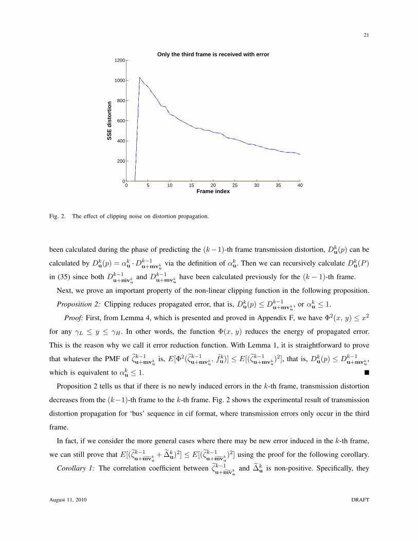
Fig. 2. The effect of clipping noise on distortion propagation.
been calculated during the phase of predicting the (k−1)-th frame transmission distortion, Dku(p) can be
calculated by Dku(p) = αk
u ·Dk−1u+mvk
uvia the definition of αk
u. Then we can recursively calculate Dku(P )
in (35) since both Dk−1u+mvk
uand Dk−1
u+mvku
have been calculated previously for the (k − 1)-th frame.
Next, we prove an important property of the non-linear clipping function in the following proposition.
Proposition 2: Clipping reduces propagated error, that is, Dku(p) ≤ Dk−1
u+mvku, or αk
u ≤ 1.
Proof: First, from Lemma 4, which is presented and proved in Appendix F, we have Φ2(x, y) ≤ x2
for any γL ≤ y ≤ γH . In other words, the function Φ(x, y) reduces the energy of propagated error.
This is the reason why we call it error reduction function. With Lemma 1, it is straightforward to prove
that whatever the PMF of ζk−1u+mvk
uis, E[Φ2(ζk−1
u+mvku, fk
u)] ≤ E[(ζk−1u+mvk
u)2], that is, Dk
u(p) ≤ Dk−1u+mvk
u,
which is equivalent to αku ≤ 1.
Proposition 2 tells us that if there is no newly induced errors in the k-th frame, transmission distortion
decreases from the (k−1)-th frame to the k-th frame. Fig. 2 shows the experimental result of transmission
distortion propagation for ‘bus’ sequence in cif format, where transmission errors only occur in the third
frame.
In fact, if we consider the more general cases where there may be new error induced in the k-th frame,
we can still prove that E[(ζk−1u+gmvk
u
+ ∆ku)2] ≤ E[(ζk−1
u+gmvku
)2] using the proof for the following corollary.
Corollary 1: The correlation coefficient between ζk−1u+gmvk
u
and ∆ku is non-positive. Specifically, they
August 11, 2010 DRAFT
22
are negatively correlated under the condition {r, p}, and uncorrelated under other conditions.
Corollary 1 is proved in Appendix H. This property is very important for designing a low complexity
algorithm to estimate propagation and clipping caused distortion in PTD, which will be presented in the
sequel paper [22].
2) Frame-level Distortion Caused by Propagated Error Plus Clipping Noise: In (35), Dk−1u+mvk
u6=
Dk−1u+mvk
udue to the non-stationarity of the error process over space. However, both the sum of Dk−1
u+mvku
over all pixels in the (k−1)-th frame and the sum of Dk−1u+mvk
uover all pixels in the (k−1)-th frame will
converge to Dk−1 due to the randomness of MV. The formula for frame-level propagation and clipping
caused distortion is given in Lemma 2.
Lemma 2: The frame-level propagation and clipping caused distortion in the k-th frame is
Dk(P ) = Dk−1 · P k(r) + Dk(p) · (1− P k(r))(1− βk), (40)
where Dk(p) , 1|V|
∑u∈Vk Dk
u(p) and P k(r) is defined in (29); βk is the percentage of I-MBs in the
k-th frame; Dk−1 is the transmission distortion in the (k − 1)-th frame.
Lemma 2 is proved in Appendix C. Define the propagation factor for the k-th frame αk , Dk(p)Dk−1 ;
then we have αk =P
u∈Vk αku·Dk−1
u+mvku
Dk−1 . Note that Dk−1u+mvk
umay be different for different pixels in the
(k − 1)-th frame due to the non-stationarity of error process over space. However, when the number
of pixels in the (k − 1)-th frame is sufficiently large, the sum of Dk−1u+mvk
uover all the pixels in the
(k−1)-th frame will converge to Dk−1. Therefore, we have αk =P
u∈Vk αku·Dk−1
u+mvkuP
u∈V Dk−1u+mvk
u
, which is a weighted
average of αku with the weight being Dk−1
u+mvku. As a result, Dk(p) ≤ Dk(P )7. However, most existing
works directly use Dk(P ) = Dk(p) in predicting transmission distortion. This is another reason why
LTI models [6], [7] under-estimate transmission distortion when there is no MV error. Details will be
discussed in Section V-B.
E. Analysis of Correlation Caused Distortion
In this subsection, we first derive the pixel-level correlation caused distortion Dku(c). Then we derive
the frame-level correlation caused distortion Dk(c).
7When the number of pixels in the (k − 1)-th frame is small,P
u∈Vk αku ·Dk−1
u+mvku
may be larger than Dk−1 although its
probability is small as observed in our experiments.
August 11, 2010 DRAFT

23
010
2030
40
0
10
20
30
40−0.5
0
0.5
1
Frame index
Temporal correlation between residuals in one trajectory
Frame index
Cor
rela
tion
coef
ficie
nt
Fig. 3. Temporal correlation between the residuals in one trajectory.
1) Pixel-level Correlation Caused Distortion: We analyze the correlation caused distortion Dku(c) at
the decoder in four different cases: i) for uk{r, m}, both εku = 0 and ξk
u = 0, so Dku(c) = 0; ii)
for uk{r, m}, ξku = 0 and Dk
u(c) = 2E[εku · (ζk−1
u+mvku
+ ∆ku{r, m})]; iii) for uk{r, m}, εk
u = 0 and
Dku(c) = 2E[ξk
u · (ζk−1u+mvk
u+ ∆k
u{r, m})]; iv) for uk{r,m}, Dku(c) = 2E[εk
u · ξku] + 2E[εk
u · (ζk−1u+mvk
u+
∆ku{r,m})]+2E[ξk
u · (ζk−1u+mvk
u+∆k
u{r,m})]. From Section IV-D1, we know ∆ku{r} = 0. So, we obtain
Dku(c) = P k
u{r, m} · 2E[εku · ζk−1
u+mvku] + P k
u{r, m} · 2E[ξku · (ζk−1
u+mvku
+ ∆ku{r,m})]
+ P ku{r,m} · (2E[εk
u · ξku] + 2E[εk
u · ζk−1u+mvk
u] + 2E[ξk
u · ζk−1u+mvk
u]).
(41)
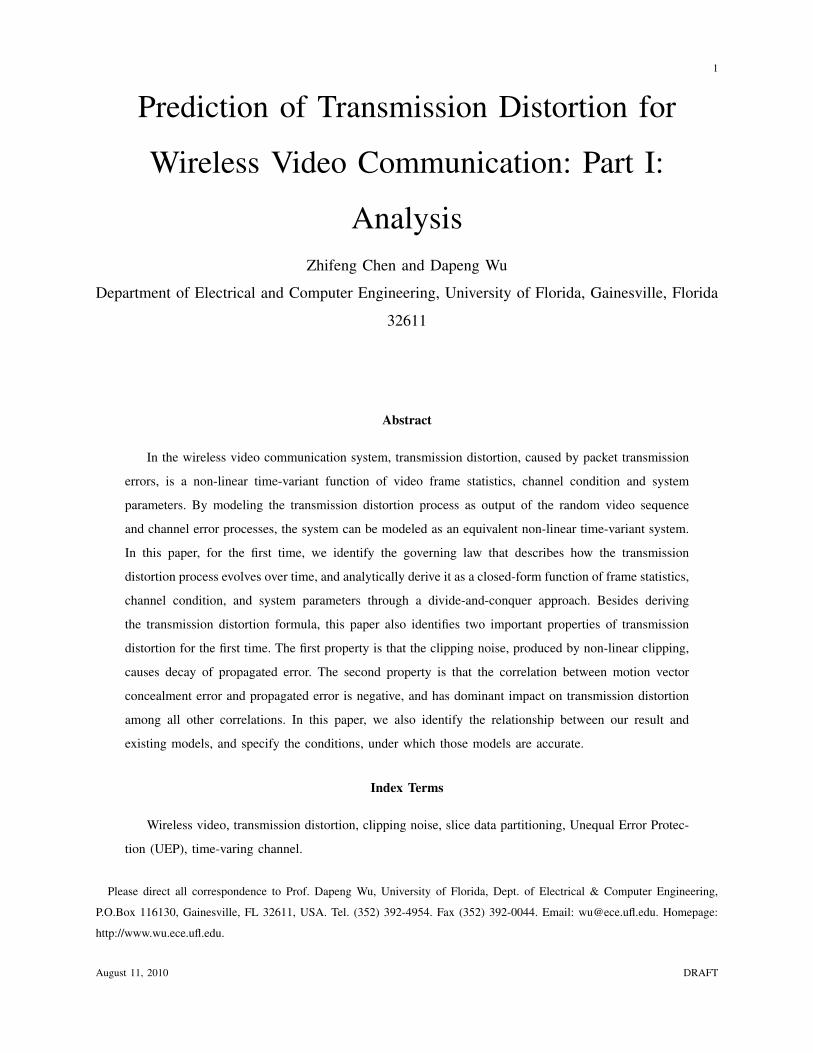
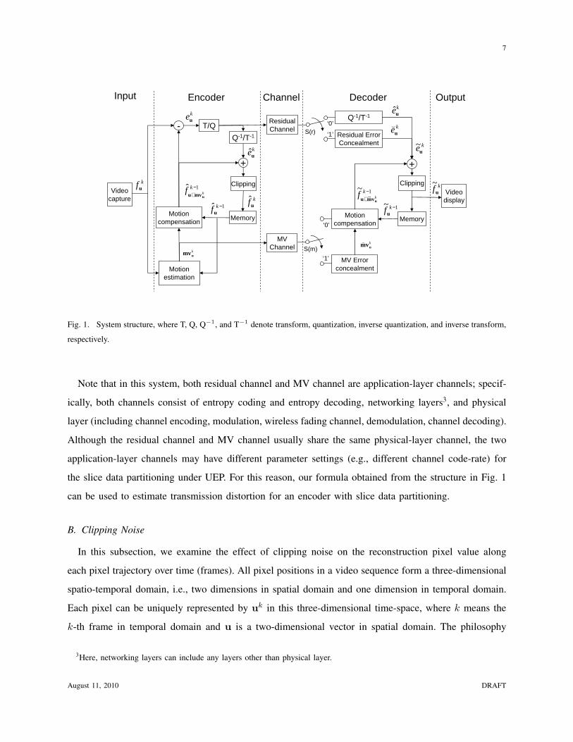
In our experiments, we find that in the trajectory of pixel uk, 1) the residual eku is approximately
uncorrelated with the residual in all other frames eiv, where i 6= k, as shown in Fig. 3 for ‘foreman’
sequence in cif format8; and 2) the residual eku is approximately uncorrelated with the MVCE of the
corresponding pixel ξku and the MVCE in all previous frames ξi
v, where i < k, as shown in Fig. 4
for ‘foreman’ sequence in cif format. Based on the above observations, we further assume that for any
i < k, eku is uncorrelated with ei
v and ξiv if vi is not in the trajectory of pixel uk, and make the following
assumption.
Assumption 5: eku is uncorrelated with ξk
u, and is uncorrelated with both eiv and ξi
v for any i < k.
8All other sequences show the same statistics for Fig. 3, Fig. 4, Fig. 5 and Fig. 6.
August 11, 2010 DRAFT
24
010
2030
40
010
2030
40−0.4
−0.2
0
0.2
0.4
MV frame index
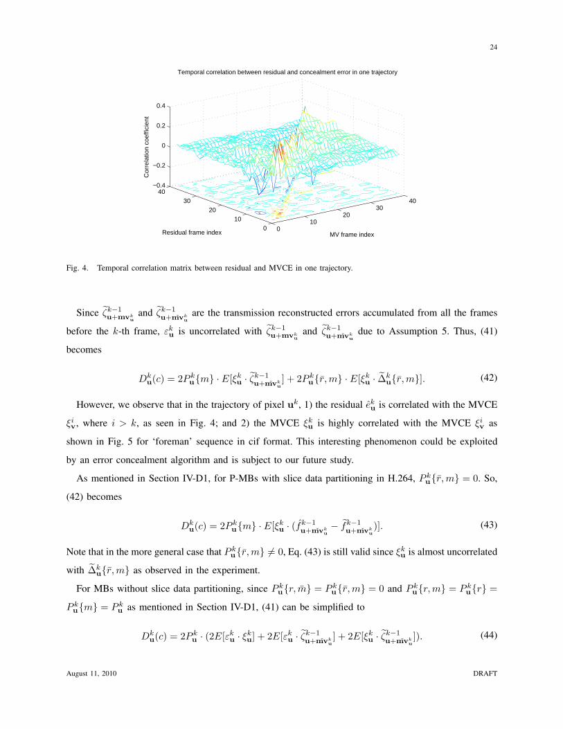
Temporal correlation between residual and concealment error in one trajectory
Residual frame index
Cor
rela
tion
coef
ficie
nt
Fig. 4. Temporal correlation matrix between residual and MVCE in one trajectory.
Since ζk−1u+mvk
uand ζk−1
u+mvku
are the transmission reconstructed errors accumulated from all the frames
before the k-th frame, εku is uncorrelated with ζk−1
u+mvku
and ζk−1u+mvk
udue to Assumption 5. Thus, (41)
becomes
Dku(c) = 2P k
u{m} · E[ξku · ζk−1
u+mvku] + 2P k
u{r, m} · E[ξku · ∆k
u{r,m}]. (42)
However, we observe that in the trajectory of pixel uk, 1) the residual eku is correlated with the MVCE
ξiv, where i > k, as seen in Fig. 4; and 2) the MVCE ξk
u is highly correlated with the MVCE ξiv as
shown in Fig. 5 for ‘foreman’ sequence in cif format. This interesting phenomenon could be exploited
by an error concealment algorithm and is subject to our future study.
As mentioned in Section IV-D1, for P-MBs with slice data partitioning in H.264, P ku{r,m} = 0. So,
(42) becomes
Dku(c) = 2P k
u{m} · E[ξku · (fk−1
u+mvku− fk−1
u+mvku)]. (43)
Note that in the more general case that P ku{r, m} 6= 0, Eq. (43) is still valid since ξk
u is almost uncorrelated
with ∆ku{r, m} as observed in the experiment.
For MBs without slice data partitioning, since P ku{r, m} = P k
u{r,m} = 0 and P ku{r,m} = P k
u{r} =
P ku{m} = P k
u as mentioned in Section IV-D1, (41) can be simplified to
Dku(c) = 2P k
u · (2E[εku · ξk
u] + 2E[εku · ζk−1
u+mvku] + 2E[ξk
u · ζk−1u+mvk
u]). (44)
August 11, 2010 DRAFT

25
010
2030
40
0
10
20
30
40−0.5
0
0.5
1
Frame index
Temporal correlation between concealment errors in one trajectory
Frame index
Cor
rela
tion
coef
ficie
nt
Fig. 5. Temporal correlation matrix between MVCEs in one trajectory.
Under Assumption 5, (44) reduces to (43).
Define λku ,
E[ξku·efk−1
u+mvku]
E[ξku·fk−1
u+mvku]; λk
u is a correlation ratio, that is, the ratio of the correlation between MVCE
and concealed reference pixel value at the decoder, to the correlation between MVCE and concealed
reference pixel value at the encoder. λku quantifies the effect of the correlation between the MVCE and
propagated error on transmission distortion.
Note that although we do not know the exact value of λku at the encoder, its range is
k−1∏
i=1
P iT(i){r, m} ≤ λk
u ≤ 1, (45)
where T(i) is the pixel position of the i-th frame in the trajectory, for example, T(k − 1) = uk + mvku
and T(k − 2) = vk−1 + mvk−1v . The left inequality in (45) holds in the extreme case that any error in
the trajectory will cause ξku and fk−1
u+mvku
to be uncorrelated, which is usually true for high motion video.
The right inequality in (45) holds in another extreme case that all errors in the trajectory do not affect
the correlation between ξku and fk−1
u+mvku, that is E[ξk
u · fk−1u+mvk
u] ≈ E[ξk
u · fk−1u+mvk
u] , which is usually true
for low motion video. The details on how to estimate λku will be presented in the sequel paper [22].
Using the definition of λku, we have the following proposition.
Proposition 3:
Dku(c) = (λk
u − 1) ·Dku(m). (46)
August 11, 2010 DRAFT
26
0 5 10 15 20 25 30 35 40
−0.25
−0.2
−0.15
−0.1
−0.05
0
0.05
0.1
0.15
0.2
0.25
Frame index
Measured ρ between ξk
uand fk−1
u+MVku
Estimated ρ between ξku
and fk−1
u+MVku
Measured ρ between ξku and fk−1
u+ˇ
MVku
Estimated ρ between ξku and fk−1
u+ˇ
MVku
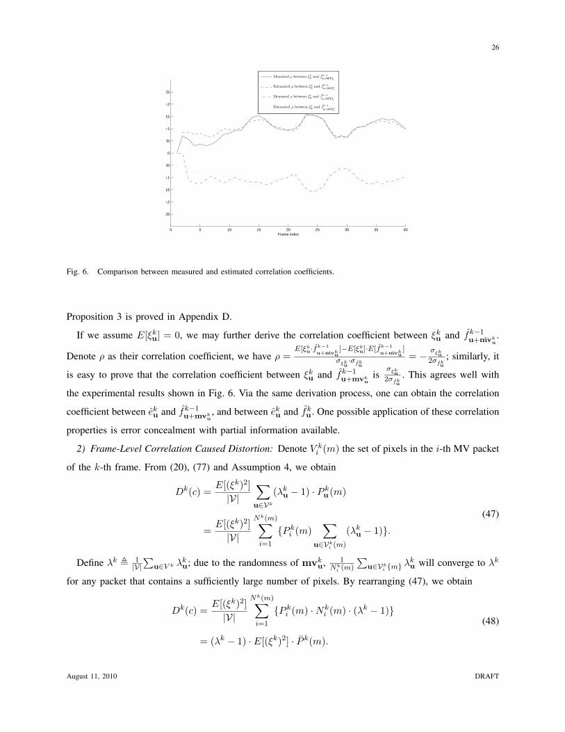
Fig. 6. Comparison between measured and estimated correlation coefficients.
Proposition 3 is proved in Appendix D.
If we assume E[ξku] = 0, we may further derive the correlation coefficient between ξk
u and fk−1u+mvk
u.
Denote ρ as their correlation coefficient, we have ρ =E[ξk
u·fk−1u+mvk
u]−E[ξk
u]·E[fk−1u+mvk
u]
σξku·σfk
u
= − σξku
2σfku
; similarly, it
is easy to prove that the correlation coefficient between ξku and fk−1
u+mvku
isσξk
u
2σfku
. This agrees well with
the experimental results shown in Fig. 6. Via the same derivation process, one can obtain the correlation
coefficient between eku and fk−1
u+mvku, and between ek
u and fku . One possible application of these correlation
properties is error concealment with partial information available.
2) Frame-Level Correlation Caused Distortion: Denote V ki (m) the set of pixels in the i-th MV packet
of the k-th frame. From (20), (77) and Assumption 4, we obtain
Dk(c) =E[(ξk)2]|V|
∑
u∈Vk
(λku − 1) · P k
u(m)
=E[(ξk)2]|V|
Nk(m)∑
i=1
{P ki (m)
∑
u∈Vki (m)
(λku − 1)}.
(47)
Define λk , 1|V|
∑u∈V k λk
u; due to the randomness of mvku, 1
Nki (m)
∑u∈Vk
i {m} λku will converge to λk
for any packet that contains a sufficiently large number of pixels. By rearranging (47), we obtain
Dk(c) =E[(ξk)2]|V|
Nk(m)∑
i=1
{P ki (m) ·Nk
i (m) · (λk − 1)}
= (λk − 1) · E[(ξk)2] · P k(m).
(48)
August 11, 2010 DRAFT
27
From (33), we know that E[(ξk)2] · P k(m) is exactly equal to Dk(m). Therefore, (48) is further
simplified to
Dk(c) = (λk − 1) ·Dk(m). (49)
F. Summary
In Section IV-A, we decomposed transmission distortion into four terms; we derived a formula for
each term in Sections IV-B through IV-E. In this section, we combine the formulae for the four terms
into a single formula.
1) Pixel-Level Transmission Distortion:
Theorem 1: Under single-reference prediction, the PTD of pixel uk is
Dku = Dk
u(r) + λku ·Dk
u(m) + P ku{r,m} ·Dk−1
u+mvku
+ P ku{r, m} ·Dk−1
u+mvku
+ P ku{r} · αk
u ·Dk−1u+mvk
u.
(50)
Proof: (50) can be obtained by plugging (24), (32), (35), and (77) into (15).
Corollary 2: Under single-reference prediction and no slice data partitioning, (50) is simplified to
Dku = P k
u · (E[(εku)2] + λk
u · E[(ξku)2] + Dk−1
u+mvku) + (1− P k
u) · αku ·Dk−1
u+mvku. (51)
2) Frame-Level Transmission Distortion:
Theorem 2: Under single-reference prediction, the FTD of the k-th frame is
Dk = Dk(r) + λk ·Dk(m) + P k(r) ·Dk−1 + (1− P k(r)) ·Dk(p) · (1− βk). (52)
Proof: (52) can be obtained by plugging (30), (33), (40) and (49) into (16).
Corollary 3: Under single-reference prediction and no slice data partitioning, the FTD of the k-th
frame is simplified to
Dk = Dk(r) + λk ·Dk(m) + P k ·Dk−1 + (1− P k) ·Dk(p) · (1− βk). (53)
V. RELATIONSHIP BETWEEN THEOREM 2 AND EXISTING TRANSMISSION DISTORTION MODELS
In this section, we will identify the relationship between Theorem 2 and their models, and specify
the conditions, under which those models are accurate. Note that in order to demonstrate the effect of
non-linear clipping on transmission distortion propagation, we disable intra update, that is, βk = 0 for
all the following cases.
August 11, 2010 DRAFT

28
A. Case 1: Only the (k−1)-th Frame Has Error, and the Subsequent Frames are All Correctly Received
In this case, the models proposed in Refs. [6], [9] state that when there is no intra coding and spatial
filtering, the propagation distortion will be the same for all the frames after the (k − 1)-th frame, i.e.,
Dn(p) = Dn−1 (∀ n ≥ k). However, this is not true as we proved in Proposition 2. Due to the clipping
function, we have αn ≤ 1 (∀ n ≥ k), i.e., Dn ≤ Dn−1 (∀ n ≥ k) in case the n-th frame is error-
free. Actually, from Appendix F, we know that the equality only holds under a very special case that
fku − γH ≤ ζk−1
u+mvku≤ fk
u − γL for all pixel u ∈ V k.
B. Case 2: Burst Errors in Consecutive Frames
In Ref. [14], authors observe that the transmission distortion caused by accumulated errors from consec-
utive frames is generally larger than the sum of those distortions caused by individual frame errors. This is
also observed in our experiment when there is no MV error. To explain this phenomenon, let us first look
at a simple case that residuals in the k-th frame are all erroneous, while the MVs in the k-th frame are all
correctly received. In this case, we obtain from (52) that Dk = Dk(r)+P k(r)·Dk−1+(1−P k(r))·Dk(p),
which is larger than the simple sum Dk(r) + Dk(p) as in the LTI model; the under-estimation caused
by the LTI model is due to Dk − (Dk(r) + Dk(p)) = (1− αk) · P k(r) ·Dk−1.
However, when MV is erroneous, the experimental result is quite different from that claimed in Ref. [14]
especially for the high motion video. In other words, the LTI model now causes over-estimation for a burst
error channel. In this case, the predicted transmission distortion can be calculated via (52) in Theorem 2
as Dk1 = Dk(r) + λk · Dk(m) + P k(r) · Dk−1
1 + (1 − P k(r)) · αk · Dk−11 , and by the LTI model as
Dk2 = Dk(r)+Dk(m)+αk ·Dk−1
2 . So, the prediction difference between Theorem 2 and the LTI model
is
Dk1 −Dk
2 = (1− αk) · P k(r) ·Dk−11 − (1− λk) · P k(m) · E[(ξk)2] + αk · (Dk−1
1 −Dk−12 ). (54)
At the beginning, D01 = D0
2 = 0, and Dk−1 << E[(ξk)2] when k is small. Therefore, the transmission
distortion caused by accumulated errors from consecutive frames will be smaller than the sum of the
distortions caused by individual frame errors, that is, Dk1 < Dk
2 . We may see from (54) that, due to the
propagation of over-estimation Dk−11 −Dk−1
2 from the (k−1)-th frame to the k-th frame, the accumulated
difference between Dk1 and Dk
2 will become larger and larger as k increases.
August 11, 2010 DRAFT

29
C. Case 3: Modeling Transmission Distortion as an Output of an LTI System with PEP as input
In Ref. [7], authors propose an LTI transmission distortion model based on their observations from
experiments. This LTI model ignores the effects of correlation between the newly induced error and the
propagated error, that is, λk = 1. This is only valid for low motion video. From (52), we obtain
Dk = Dk(r) + Dk(m) + (P k(r) + (1− P k(r)) · αk) ·Dk−1. (55)
Let ηk = P k(r)+(1− P k(r)) ·αk. If 1) there is no slice data partitioning, i.e., P k(m) = P k(r) = P k,
and 2) P k(r) = P k(r) (which means one frame is transmitted in one packet, or different packets
experience the same channel condition), then (55) becomes Dk = {E[(ξk)2]+E[(εk)2]}·P k +ηk ·Dk−1.
Let Ek , E[(ξk)2] + E[(εk)2]. Then the recursive formula results in
Dk =k∑
l=k−L
[(k∏
i=l+1
ηi) · (El · P l)], (56)
where L is the time interval between the k-th frame and the latest correctly received frame.
Denote the system by an operator H that maps the error input sequence {P k}, as a function of frame
index k, to the distortion output sequence {Dk}. Since generally Dk(p) is a nonlinear function of Dk−1,
as a ratio of Dk(p) and Dk−1, αk is still a function of Dk−1. As a result, ηk is a function of Dk−1.
That means the operator H is non-linear, i.e., the system is non-linear. In addition, since αk varies from
frame to frame as mentioned in Section IV-D2, the system is time-variant. In summary, H is generally
a non-linear time-variant system.
The LTI model assumes that 1) the operator H is linear, that is, H(a·P k1 +b·P k
2 ) = a·H(P k1 )+b·H(P k
2 ),
which is valid only when ηk does not depend on Dk−1; and 2) the operator H is time-invariant, that is,
Dk+δ = H(P k+δ), which is valid only when ηk is constant, i.e., both P k(r) and αk are constant. Under
these two assumptions, we have ηi = η, and we obtain∏k
i=l+1 ηi = (η)k−l. Let h[k] = (η)k, where h[k]
is the impulse response of the LTI model; then we obtain
Dk =k∑
l=k−L
[h[k − l] · (El · P l)]. (57)
From Proposition 2, it is easy to prove that 0 ≤ η ≤ 1; so h[k] is a decreasing function of time. We see
that (57) is a convolution between the error input sequence and the system impulse response. Actually, if
we let h[k] = e−γk, where γ = − log η, it is exactly the formula proposed in Ref. [7]. Note that (57) is a
very special case of (52) with the following limitations: 1) the video content has to be of low motion; 2)
there is no slice data partitioning or all pixels in the same frame experience the same channel condition;
3) ηk is a constant, that is, both P k(r) and the propagation factor αk are constant, which requires the
August 11, 2010 DRAFT
30
probability distributions of reconstructed pixel values in all frames should be the same. Note that the
physical meaning of ηk is not the actual propagation factor, but it is just a notation for simplifying the
formula.
VI. PTD AND FTD UNDER MULTI-REFERENCE PREDICTION
The PTD and FTD formulae in Section IV are for single-reference prediction. In this section, we
extend the formulae to multi-reference prediction.
A. Pixel-level Distortion under Multi-Reference Prediction
If multiple frames are allowed to be the references for motion estimation, the reconstructed pixel value
at the encoder in (1) becomes
fku = Γ(fk−j
u+mvku
+ eku). (58)
For the reconstructed pixel value at the decoder in (3), it is a bit different as below.
fku = Γ(fk−j′
u+gmvku
+ eku). (59)
If mvku is correctly received, mvk
u = mvku and fk−j′
u+gmvku
= fk−ju+mvk
u. However, if mvk
u is received with
error, the concealed MV has no difference from the single-reference case, that is, mvku = mvk
u and
fk−j′
u+gmvku
= fk−1u+mvk
u.
As a result, (12) becomes
ζku = (ek
u + fk−ju+mvk
u− ∆k
u)− (eku + fk−j′
u+gmvku
− ∆ku)
= (eku − ek
u) + (fk−ju+mvk
u− fk−j′
u+gmvku
) + (fk−j′
u+gmvku
− fk−j′
u+gmvku
)− (∆ku − ∆k
u).(60)
Following the same derivation process from Section IV-A to Section IV-E, the formulae for PTD under
multi-reference prediction are the same as those under single-reference prediction except the following
changes: 1) MVCE ξku , fk−j
u+mvku− fk−j′
u+gmvku
and clipping noise ∆ku , (fk−j′
u+gmvku
+ eku)−Γ(fk−j′
u+gmvku
+ eku);
2) Dku(m) and Dk
u(c) are given by (32) and (46), respectively, with a new definition of ξku , fk−j
u+mvku−
fk−1u+mvk
u; 3) Dk
u(p) , E[(ζk−ju+mvk
u+ ∆k
u{r, m})2], αku , Dk
u(p)
Dk−j
u+mvku
and
Dku(P ) = P k
u{r,m} ·Dk−1u+mvk
u+ P k
u{r, m} ·Dk−ju+mvk
u+ P k
u{r} ·Dku(p), (61)
compared to (35). The generalization of PTD formulae to multi-reference prediction is straightforward
since the multi-reference prediction case just has a larger set of reference pixels than the single-reference
case. Following the same derivation process, we have the following general theorem for PTD.
August 11, 2010 DRAFT
31
Theorem 3: Under multi-reference prediction, the PTD of pixel uk is
Dku = Dk
u(r) + λku ·Dk
u(m) + P ku{r,m} ·Dk−1
u+mvku
+ P ku{r, m} ·Dk−j
u+mvku
+ P ku{r} · αk
u ·Dk−ju+mvk
u.
(62)
Corollary 4: Under multi-reference prediction and no slice data partitioning, (62) is simplified to
Dku = P k
u · (E[(εku)2] + λk
u · E[(ξku)2] + Dk−1
u+mvku) + (1− P k
u) · αku ·Dk−j
u+mvku. (63)
B. Frame-level Distortion under Multi-Reference Prediction
Under multi-reference prediction, each block typically is allowed to choose its reference block in-
dependently; hence, different pixels in the same frame may have different reference frames. Define
V k(j) , {uk : uk = vk−j −mvku}, where j ∈ {1, 2, ..., J} and J is the number of reference frames;
i.e., V k(j) is the set of the pixels in the k-th frame, whose reference pixels are in the (k − j)-th frame.
Obviously,⋃J
j=1 V k(j) = V k and⋂J
j=1 V k(j) = ∅. Define wk(j) , |Vk(j)||Vk| . Note that V k and V k(j)
have the similar physical meanings but only the different cardinalities.
Dk(m) and Dk(c) are given by (33) and (49), respectively, with a new definition of ξk(j) , {ξku :
ξku = fk−j
u+mvku− fk−1
u+mvku}. and ξk =
∑Jj=1 wk(j) · ξk(j). Define the propagation factor of V k(j) by
αk(j) ,P
u∈V k(j) αku·Dk−j
u+mvkuP
u∈V k(j) Dk−j
u+mvku
. The following lemma gives the formula for Dk(P ).
Lemma 3: The frame-level propagation and clipping caused distortion in the k-th frame for the multi-
reference case is
Dk(P ) = Dk−1 · P k{r,m}+J∑
j=1
(P k(j){r, m} · wk(j) ·Dk−j)
+ (1− βk) ·J∑
j=1
(P k(j){r} · wk(j) · αk(j) ·Dk−j),
(64)
where βk is the percentage of I-MBs in the k-th frame; P k(j){r, m} is the weighted average of joint
PEPs of event {r, m} for the j-th sub-frame in the k-th frame. P k(j){r} is the weighted average of PEP
of event {r} for the j-th sub-frame in the k-th frame.
Lemma 3 is proved in Appendix E. With Lemma 3, we have the following general theorem for FTD.
Theorem 4: Under multi-reference prediction, the FTD of the k-th frame is
Dk = Dk(r) + λk ·Dk(m) + Dk−1 · P k{r,m}+J∑
j=1
(P k(j){r, m} · wk(j) ·Dk−j)
+ (1− βk) ·J∑
j=1
(P k(j){r} · wk(j) · αk(j) ·Dk−j).
(65)
August 11, 2010 DRAFT

32
Proof: (65) can be obtained by plugging (30), (33), (64) and (49) into (16).
It is easy to prove that (52) in Theorem 2 is a special case of (65) with J = 1 and wk(j) = 1. It is also
easy to prove that (62) in Theorem 3 is a special case of (65) with |V| = 1.
Corollary 5: Under multi-reference prediction and no slice data partitioning, (65) is simplified to
Dk = Dk(r) + λk ·Dk(m) + Dk−1 · P k{r}+ (1− βk) ·J∑
j=1
(P k(j){r} · wk(j) · αk(j) ·Dk−j). (66)
VII. CONCLUSION
In this paper, we derived the transmission distortion formulae for wireless video communication
systems. With consideration of spatio-temporal correlation, nonlinear codec and time-varying channel,
our formulae provide, for the first time, the following capabilities: 1) support of distortion prediction
at different levels (e.g., pixel/frame/GOP level), 2) support of accurate multi-reference prediction, 3)
support of slice data partitioning, 4) support of arbitrary slice-level packetization with FMO mechanism,
5) being applicable to time-varying channels, 6) one unified formula for both I-MB and P-MB, and
7) support of both low motion and high motion video sequences. Besides deriving the transmission
distortion formulae, this paper also identified two important properties of transmission distortion for the
first time: 1) clipping noise, produced by non-linear clipping, causes decay of propagated error; 2) the
correlation between motion vector concealment error and propagated error is negative, and has dominant
impact on transmission distortion, among all the correlations between any two of the four components
in transmission error. We also discussed the relationship between our formula and existing models. In
the sequel paper [22], we use the formulae derived in this paper to design algorithms for estimating
pixel-level and frame-level transmission distortion and apply the algorithms to video codec design; we
also verify the accuracy of the formulae derived in this paper through experiments; the application of
these formulae shows superior performance over existing models.
ACKNOWLEDGMENTS
This work was supported in part by an Intel gift, the US National Science Foundation under grant
DBI-0529012 and CNS-0643731. The authors would like to thank Jun Xu and Qian Chen for many
fruitful discussions related to this work and suggestions that helped to improve the presentation of this
paper.
August 11, 2010 DRAFT

33
APPENDIX
A. Proof of Lemma 1
Proof: From (11) and (13), we obtain fk−1u+gmvk
u
+ eku = fk
u − ξku − εk
u − ζk−1u+gmvk
u
,
Together with (9), we obtain
∆ku = (fk
u − ξku − εk
u − ζk−1u+gmvk
u
)− Γ(fku − ξk
u − εku − ζk−1
u+gmvku
). (67)
So, ζk−1u+gmvk
u
+ ∆ku = (fk
u − ξku − εk
u)− Γ(fku − ξk
u − εku − ζk−1
u+gmvku
), and
Dku(P ) = E[(ζk−1
u+gmvku
+ ∆ku)2] = E[Φ2(ζk−1
u+gmvku
, fku − ξk
u − εku)]. (68)
We know from the definition that Dku(p) is a special case of Dk
u(P ) under the condition {r, m}, which
means eku = ek
u, i.e. εku = 0, and mvk
u = mvku, i.e. ξk
u = 0. Therefore, we obtain
Dku(p) = E[Φ2(ζk−1
u+mvku, fk
u)]. (69)
B. Proof of Proposition 1
Proof: The probability density function of the random variable having a Laplacian distribution is
f(x|µ, b) = 12b exp
(− |x−µ|
b
). Since µ = 0, we have E[x2] = 2b2, and from (38), we obtain
E[x2]− E[Φ2(x, y)] =∫ +∞
y−γL
(x2 − (y − γL)2)12b
e−x
b dx +∫ y−γH
−∞[x2 − (y − γH)2]
12b
ex
b dx
= e−y−γL
b ((y − γL) · b + b2) + e−γH−y
b ((γH − y) · b + b2).
(70)
From the definition of propagation factor, we obtain α = E[Φ2(x, y)]E[x2] = 1 − 1
2e−y−γL
b (y−γL
b + 1) −12e−
γH−y
b (γH−yb + 1).
C. Proof of Lemma 2
Proof: For P-MBs with slice data partioning, from (19) and (35) we obtain
Dk(P ) =1|V|
∑
u∈Vk
(P ku{r,m} ·Dk−1
u+mvku) +
1|V|
∑
u∈Vk
(P ku{r, m} ·Dk−1
u+mvku) +
1|V|
∑
u∈Vk
(P ku{r} ·Dk
u(p)).
(71)
Denote V ki {r,m} the set of pixels in the k-th frame with the same XEP P k
i {r,m}; denote Nki {r,m}
the number of pixels in V ki {r,m}; denote Nk{r,m} the number of sets with different XEP P k
i {r,m}in the k-th frame.
August 11, 2010 DRAFT
34
We have
1|V|
∑
u∈Vk
(P ku{r,m} ·Dk−1
u+mvku) =
1|V|
Nk{r,m}∑
i=1
(P ki {r,m}
∑
u∈Vki {r,m}
Dk−1u+mvk
u). (72)
For large Nki {r,m}, we have 1
Nki {r,m}
∑u∈Vk
i {r,m}Dk−1u+mvk
uconverges to Dk−1, so the first term in the
right-hand side in (71) is Dk−1 · P k{r,m}, where P k{r,m} = 1|V|
∑Nk{r,m}i=1 (P k
i {r,m} ·Nki {r,m}).
Following the same process, we obtain the second term in the right-hand side in (71) as Dk−1·P k{r, m},
where P k{r, m} = 1|V|
∑Nk{r,m}i=1 (P k
i {r, m} ·Nki {r, m}); and
1|V|
∑
u∈Vk
(P ku{r} ·Dk
u(p)) =1|V|
Nk{r}∑
i=1
(P ki {r}
∑
u∈Vki {r}
Dku(p)). (73)
For large Nki {r}, we have 1
Nki {r}
∑u∈Vk
i {r}Dku(p) converges to Dk(p), so the third term in the right-hand
side in (71) is Dk(p) · (1− P k(r)).
Note that P ki {r,m}+ P k
i {r, m} = P ki {r} and Nk
i {r,m} = Nki {r, m}. So, we obtain
Dk(P ) = Dk−1 · P k(r) + Dk(p) · (1− P k(r)). (74)
For P-MBs without slice data partitioning, it is straightforward to acquire (74) from (36). For I-MBs,
from (37), it is also easy to obtain Dk(P ) = Dk−1 · P k(r). So, together with (74), we obtain (40).
D. Proof of Proposition 3
Proof: Using the definition of λku, (43) becomes
Dku(c) = 2P k
u{m} · (1− λku) · E[ξk
u · fk−1u+mvk
u]. (75)
Under the condition that the distance between mvku and mvk
u is small, for example, inside the same MB,
the statistics of fk−1u+mvk
uand fk−1
u+mvku
are almost the same. Therefore, we may assume E[(fk−1u+mvk
u)2] =
E[(fk−1u+mvk
u)2].
Since ξku = fk−1
u+mvku− fk−1
u+mvku, we have
E[(fk−1u+mvk
u)2] = E[(fk−1
u+mvku)2]
= E[(ξku + fk−1
u+mvku)2],
(76)
and therefore E[ξku · fk−1
u+mvku] = −E[(ξk
u)2]2
9.
9Note that following the same derivation process, we can prove E[ξku · fk−1
u+mvku] =
E[(ξku)2]
2.
August 11, 2010 DRAFT

35
Therefore, (75) can be simplify as
Dku(c) = (λk
u − 1) · E[(ξku)2] · P k
u(m). (77)
From (32), we know that E[(ξku)2]·P k
u(m) is exactly equal to Dku(m). Therefore, (77) is further simplified
to (46).
E. Proof of Lemma 3
Proof: For P-MBs with slice data partioning, from (19) and (61) we obtain
Dk(P ) =1|V|
∑
u∈Vk
(P ku{r,m} ·Dk−1
u+mvku) +
1|V|
∑
u∈Vk
(P ku{r, m} ·Dk−j
u+mvku) +
1|V|
∑
u∈Vk
(P ku{r} ·Dk
u(p)).
(78)
The first term in the right-hand side in (78) is exactly the same as the first term in the right-hand side
in (71), that is, it equal to Dk−1 · P k{r,m}, where P k{r,m} = 1|V|
∑Nk{r,m}i=1 (P k
i {r,m} ·Nki {r,m}).
Denote V ki (j){r, m} the set of pixels using the same reference frame k− j in the k-th frame with the
same XEP P ki (j){r, m}; denote Nk
i (j){r, m} the number of pixels in V ki (j){r, m}; denote Nk(j){r, m}
the number of sets with different XEP P ki (j){r, m} but the same reference frame k−j in the k-th frame.
We have
1|V|
∑
u∈Vk
(P ku{r, m} ·Dk−j
u+mvku) =
1|V|
Nk(j){r,m}∑
i=1
(P ki (j){r, m}
J∑
j=1
∑
u∈Vki (j){r,m}
Dk−ju+mvk
u). (79)
For large Nki (j){r, m}, we have 1
Nki (j){r,m}
∑u∈Vk
i (j){r,m}Dk−ju+mvk
uconverges to Dk−j , so (79) becomes
1|V|
∑
u∈Vk
(P ku{r, m} ·Dk−j
u+mvku) =
1|V|
Nk(j){r,m}∑
i=1
(P ki (j){r, m}
J∑
j=1
Nki (j){r, m} ·Dk−j). (80)
Similar to the definition in (29), we define the weighted average over joint PEPs, of event that residual
is received with error and MV is received without error, for the set of pixels using the same reference
frame k − j in the k-th frame as
P k(j){r, m} , 1|Vk(j)|
Nk(j){r,m}∑
i=1
(P ki (j){r, m} ·Nk
i (j){r, m}). (81)
We have
1|V|
∑
u∈Vk
(P ku{r, m} ·Dk−j
u+mvku) =
1|V|
J∑
j=1
(P k(j){r, m} · |Vk(j)| ·Dk−j)
=J∑
j=1
(P k(j){r, m} · wk(j) ·Dk−j).
(82)
August 11, 2010 DRAFT
36
Following the same derivation process, we obtain
1|V|
∑
u∈Vk
(P ku{r} ·Dk
u(p)) =J∑
j=1
(P k(j){r} · wk(j) · αk(j) ·Dk−j), (83)
where
P k(j){r} , 1|Vk(j)|
Nk(j){r}∑
i=1
(P ki (j){r} ·Nk
i (j){r}) (84)
is the weighted average over joint PEPs, of event that residual is received without error, for the set of
pixels using the same reference frame k − j in the k-th frame.
Therefore, we obtain
Dk(P ) = Dk−1 · P k{r,m}+J∑
j=1
(P k(j){r, m} · wk(j) ·Dk−j) +J∑
j=1
(P k(j){r} · wk(j) · αk(j) ·Dk−j).
(85)
For P-MBs without slice data partitioning, P k{r,m} = P k{r} and P k(j){r, m} = 0, therefore we have
Dk(P ) = Dk−1 · P k{r}+J∑
j=1
(P k(j){r} · wk(j) · αk(j) ·Dk−j). (86)
For I-MBs, from (37), it is also easy to obtain Dk(P ) = Dk−1 · P k(r). So, together with (85), we obtain
(64).
F. Lemma 4 and Its Proof
To prove Proposition 2, we need to use the following lemma.
Lemma 4: The error reduction function Φ(x, y) satisfies Φ2(x, y) ≤ x2 for any γL ≤ y ≤ γH .
Proof: From the definition in (38), we obtain
Φ2(x, y)− x2 =
(y − γL)2 − x2, x > y − γL
0, y − γH ≤ x ≤ y − γL
(y − γH)2 − x2, x < y − γH .
(87)
Since y ≥ γL, we obtain (y − γL)2 < x2 when x > y − γL. Similarly, since y ≤ γH , we obtain
(y − γH)2 < x2 when x < y − γH . Therefore Φ2(x, y) − x2 ≤ 0 for γL ≤ y ≤ γH . Fig. 7 shows a
pictorial example of the case that γH = 255, γL = 0 and y = 100.
August 11, 2010 DRAFT

37
−300 −200 −100 0 100 200 3000
1
2
3
4
5
6
7
8
9x 10
4
x
y=100, γH
=255, γL=0
x2
Φ2(x, y)
Fig. 7. Comparison of Φ2(x, y) and x2.
G. Lemma 5 and Its Proof
Before presenting the proof, we first give the definition of Ideal Codec.
Definition 1: Ideal Codec: both the true MV and concealed MV are within the search range, and the
position pointed by the true MV, i.e., u + mvku, is the best reference pixel, under the MMSE criteria,
for fku within the whole search range Vk−1
SR , that is, v = arg minv∈Vk−1
SR
{(fku − fk−1
v )2}.
To prove Corollary 1, we need to use the following lemma.
Lemma 5: In an ideal codec, ∆ku{p} = 0, In other words, if there is no propagated error, the clipping
noise for the pixel uk at the decoder is always zero no matter what kind of error event occurs in the k-th
frame.
Proof: In an ideal codec, we have (eku)2 = (fk
u−fk−1u+mvk
u)2 ≤ (fk
u−fk−1u+mvk
u)2. Due to the spatial and
temporal continuity of the natural video, we can prove by contradiction that in an ideal codec fku−fk−1
u+mvku
and fku − fk−1
u+mvku
have the same sign, that is either
fku − fk−1
u+mvku≥ ek
u ≥ 0, or fku − fk−1
u+mvku≤ ek
u ≤ 0. (88)
If the sign of fku − fk−1
u+mvku
and fku − fk−1
u+mvku
is not the same, then due to the spatial and temporal
continuity of the input video, there exists a better position v ∈ Vk−1 between mvku and mvk
u, and
August 11, 2010 DRAFT

38
therefore within the search range, so that (eku)2 ≥ (fk
u − fk−1v )2. In this case, encoder will choose v as
the best reference pixel within the search range. This contradicts the assumption that the best reference
pixel is u + mvku within the search range.
Therefore, from (88), we obtain
fku ≥ fk−1
u+mvku
+ eku ≥ fk−1
u+mvku, or fk
u ≤ fk−1u+mvk
u+ ek
u ≤ fk−1u+mvk
u. (89)
Since both fku and fk−1
u+mvku
are reconstructed pixel value, they are within the range γH ≥ fku, fk−1
u+mvku≥
γL. From (89), we have γH ≥ fk−1u+mvk
u+ ek
u ≥ γL, and thus Γ(fk−1u+mvk
u+ ek
u) = fk−1u+mvk
u+ ek
u. As a
result, we obtain ∆ku{r, m, p} = (fk−1
u+mvku
+ eku)− Γ(fk−1
u+mvku
+ eku) = 0.
Since ∆ku{r, m, p} = ∆k
u = 0, and from Section IV-D1, we know that ∆ku{r, p} = 0, hence we obtain
∆ku{p} = 0.
Remark 1: Note that Lemma 5 is proved under the assumption of pixel-level motion estimation. In
a practical encoder, block-level motion estimation is adopted with the criterion of minimizing the MSE
of the whole block, e.g., in H.263, or minimizing the cost of residual bits and MV bits, e.g., in H.264.
Therefore, some reference pixels in the block may not be the best reference pixel within the search range.
On the other hand, Rate Distortion Optimization (RDO) as used in H.264 may also cause some reference
pixels not to be the best reference pixels. However, the experiment results for all the test video sequences
show that the probability of ∆ku{r, m, p} 6= 0 is negligible.
H. Proof of Corollary 1
Proof: From (67), we obtain ∆ku{p} = (fk
u − ξku− εk
u)−Γ(fku − ξk
u− εku). Together with Lemma 5,
which is presented and proved in Appendix G, we have γL ≤ fku − ξk
u − εku ≤ γH . From Lemma 4 in
Appendix F, we have Φ2(x, y) ≤ x2 for any γL ≤ y ≤ γH ; together with (68), it is straightforward to
prove that E[(ζk−1u+gmvk
u
+ ∆ku)2] ≤ E[(ζk−1
u+gmvku
)2]. By expanding E[(ζk−1u+gmvk
u
+ ∆ku)2], we obtain
E[ζk−1u+gmvk
u
· ∆ku] ≤ −1
2E[(∆k
u)2] ≤ 0. (90)
The physical meaning of (90) is that ζk−1u+gmvk
u
and ∆ku are negatively correlated if ∆k
u 6= 0. Since
∆ku{r} = 0 as noted in Section IV-D1 and ∆k
u{p} = 0 as proved in Lemma 5, we know that ∆ku 6= 0 is
valid only for the error events {r, m, p} and {r, m, p}, and ∆ku = 0 for any other error event. In other
words, ζk−1u+gmvk
u
and ∆ku are negatively correlated under the condition {r, p}, and they are uncorrelated
under other conditions.
August 11, 2010 DRAFT

39
REFERENCES
[1] C. E. Shannon, “Coding theorems for a discrete source with a fidelity criterion,” IRE Nat. Conv. Rec. Part, vol. 4, pp.
142–163, 1959.
[2] T. Berger and J. Gibson, “Lossy source coding,” IEEE Transactions on Information Theory, vol. 44, no. 6, pp. 2693–2723,
1998.
[3] R. Zhang, S. L. Regunathan, and K. Rose, “Video coding with optimal inter/intra-mode switching for packet loss resilience,”
IEEE Journal on Selected Areas in Communications, vol. 18, no. 6, pp. 966–976, Jun. 2000.
[4] T. Stockhammer, M. Hannuksela, and T. Wiegand, “H. 264/AVC in wireless environments,” IEEE Transactions on Circuits
and Systems for Video Technology, vol. 13, no. 7, pp. 657–673, 2003.
[5] T. Stockhammer, T. Wiegand, and S. Wenger, “Optimized transmission of h.26l/jvt coded video over packet-lossy networks,”
in IEEE ICIP, 2002.
[6] K. Stuhlmuller, N. Farber, M. Link, and B. Girod, “Analysis of video transmission over lossy channels,” IEEE Journal on
Selected Areas in Communications, vol. 18, pp. 1012–1032, Jun. 2000.
[7] J. U. Dani, Z. He, and H. Xiong, “Transmission distortion modeling for wireless video communication,” in Proceedings
of IEEE Global Telecommunications Conference (GLOBECOM’05), 2005.
[8] Z. He, J. Cai, and C. W. Chen, “Joint source channel rate-distortion analysis for adaptive mode selection and rate control
in wireless video coding,” IEEE Transactions on Circuits and System for Video Technology, special issue on wireless video,
vol. 12, pp. 511–523, Jun. 2002.
[9] Y. Wang, Z. Wu, and J. M. Boyce, “Modeling of transmission-loss-induced distortion in decoded video,” IEEE Transactions
on Circuits and Systems for Video Technology, vol. 16, no. 6, pp. 716–732, Jun. 2006.
[10] J. Chakareski, J. Apostolopoulos, W.-T. Tan, S. Wee, and B. Girod, “Distortion chains for predicting the video distortion
for general packet loss patterns,” in Proc. ICASSP, 2004.
[11] J. Chakareski, J. Apostolopoulos, S. Wee, W.-T. Tan, and B. Girod, “Rate-distortion hint tracks for adaptive video streaming,”
IEEE transactions on circuits and systems for video technology, vol. 15, no. 10, pp. 1257–1269, 2005.
[12] C. Zhang, H. Yang, S. Yu, and X. Yang, “GOP-level transmission distortion modeling for mobile streaming video,” Signal
Processing: Image Communication, 2007.
[13] M. T. Ivrlac, L. U. Choi, E. Steinbach, and J. A. Nossek, “Models and analysis of streaming video transmission over
wireless fading channels,” Signal Processing: Image Communication, vol. 24, no. 8, pp. 651–665, Sep. 2009.
[14] Y. J. Liang, J. G. Apostolopoulos, and B. Girod, “Analysis of packet loss for compressed video: Effect of burst losses and
correlation between error frames,” IEEE Transactions on Circuits and Systems for Video Technology, vol. 18, no. 7, pp.
861–874, Jul. 2008.
[15] H. Yang and K. Rose, “Advances in recursive per-pixel end-to-end distortion estimation for robust video coding in H.
264/AVC,” IEEE Transactions on Circuits and Systems for Video Technology, vol. 17, no. 7, p. 845, 2007.
[16] “H.264/AVC reference software JM14.0,” May. 2008. [Online]. Available: http://iphome.hhi.de/suehring/tml/download
[17] A. Goldsmith, Wireless Communications. Cambridge University Press, 2005.
[18] S. Wenger, “H.264/AVC over IP,” IEEE Transactions on Circuits and Systems for Video Technology, vol. 13, no. 7, pp.
645– 656, Jul. 2003.
[19] T. Wiegand, G. J. Sullivan, G. Bjontegaard, and A. Luthra, “Overview of the h.264/AVC video coding standard,” IEEE
Transactions on Circuits and Systems for Video Technology, vol. 13, no. 7, pp. 560–576, Jul. 2003.
August 11, 2010 DRAFT

40
[20] D. Agrafiotis, D. R. Bull, and C. N. Canagarajah, “Enhanced error concealment with mode selection,” IEEE Transactions
on Circuits and Systems for Video Technology, vol. 16, no. 8, pp. 960–973, Aug. 2006.
[21] ITU-T Series H: Audiovidual and Multimedia Systems, Advanced video coding for generic audiovisual services, Nov. 2007.
[22] Z. Chen and D. Wu, “Prediction of Transmission Distortion for Wireless Video Communication: Part II: Algorithm and
Application,” 2010, http://www.wu.ece.ufl.edu/mypapers/journal-2.pdf.
August 11, 2010 DRAFT
Recommended