Physics of uncertainty, the Gibbs paradox and indistinguishable particles
Demetris Koutsoyiannis
Department of Water Resources and Environmental Engineering, School of Civil
Engineering, National Technical University of Athens, Greece ([email protected] –
http://www.itia.ntua.gr/dk)
Abstract. The idea that, in the microscopic world, particles are indistinguishable,
interchangeable and without identity has been central in quantum physics. The same
idea has been enrolled in statistical thermodynamics even in a classical framework of
analysis to make theoretical results agree with experience. In thermodynamics of
gases, this hypothesis is associated with several problems, logical and technical. For
this case, an alternative theoretical framework is provided, replacing the
indistinguishability hypothesis with standard probability and statistics. In this
framework, entropy is a probabilistic notion applied to thermodynamic systems and is
not extensive per se. Rather, the extensive entropy used in thermodynamics is the
difference of two probabilistic entropies. According to this simple view, no
paradoxical behaviours, such as the Gibbs paradox, appear. Such a simple
probabilistic view within a classical physical framework, in which entropy is none
other than uncertainty applicable irrespective of particle size, enables generalization of
mathematical descriptions of processes across any type and scale of systems ruled by
uncertainty.
Keywords. Uncertainty; Probability; Entropy; Gibbs paradox; Extensivity;
Indistinguishability; Maxwell-Boltzmann statistics.
1. Introduction
Φύσις κρύπτεσθαι φιλεῖ (Nature loves to hide; Heraclitus)
The idea that in the microscopic world the particles are indistinguishable, interchangeable and without
identity has been central in quantum physics and is supported by empirical evidence. Two objects are
identical whenever they have the same architecture and the same values of quantum numbers,
expressing their state. In typical quantum mechanical systems, the number of states (dimension of
Hilbert space) that describe what may happen in a finite volume is always finite (usually small) and
therefore the probability of having particles in identical states is non-zero.
The same idea has been enrolled in statistical thermodynamics even in a classical framework of
analysis [e.g. 1, 2, 3, 4] to help make theoretical results to agree with experience or perception, as well
as with pre-existing thermodynamic results. Namely, the indistinguishability hypothesis has been
central in determining the entropy in the kinetic theory of gases. In this case, the idea has been
accepted despite absence of direct experimental evidence supporting it [e.g., 5, p. 11]. It is well known
that in the kinetic theory of gases the energy and momentum are taken to be continuous variables, as in
classical physics, rather than discrete variables taking on a finite number of values as in quantum
physics. Therefore, the probability that any two particles in motion have the same velocity, momentum
and energy is zero and this can hardly justify their indistinguishability (even if the architecture of
particles is identical).
The indistinguishability hypothesis is not about whether or not we can distinguish or label particles.
It goes far beyond the fact that the particles are identical, implying that this property affects the
probabilistic behaviour of particles and the entropy of the system. Thus, the indistinguishability
hypothesis has resulted in three different probabilistic behaviours or models, typically referred to as
“statistics”, each one labelled by two names of some of the most respected physicists in history. All

2
three depart from standard probability and statistics, which we use in all sciences, including physics of
the macroscopic world. The typical probability-theoretic problem of placing N particles into M boxes
(representing particle states or locations) can serve as a cue for distinguishing the three models from
each other, as well from the standard probability model. Specifically, the number W of possible ways
of placing the particles according to the different models are [4, pp. 259-264, 319-320; 5 pp. 11, 61]:
Standard probabilistic model:
W = M N
(1)
Maxwell-Boltzmann statistics (lacking clear definition; see section 7):
WMB = W
N! =
M N
N! (2)
Bose-Einstein statistics (each of N indistinguishable bosons occupies each of M states with no
restriction on the occupation number in each state):
WBE =
N + M – 1
N =
(N + M – 1)!
N! (M – 1)! (3)
Fermi-Dirac statistics (each of N indistinguishable femions occupies each of M > N states with
the restriction that no more than one particle can occupy a specific state):
WFD =
M
N =
M!
N! (M – N)! (4)
In particular, the notion that triggered the introduction of Maxwell-Boltzmann statistics, which is
the focus of this study, was the entropy of systems of gas molecules, in which the typical model
resulted in an entropic form that was non-extensive, while classical thermodynamics demands that the
entropy be extensive. Here, an attempt is made to show that the typical probabilistic model (equation
(1)) can be reconciled with classical thermodynamics of gases without invoking indistinguishability,
and, at the same time, resolving in a natural way paradoxical results (the Gibbs paradox) associated
with indistinguishability. It is stressed that the study is focused on the inconsistencies of Maxwell-
Boltzmann statistics with respect to thermodynamics of gases and does not extend to phenomena
commonly treated by Bose-Einstein statistics and Fermi-Dirac statistics. It is also noted that the
rationale that the indistinguishability hypothesis should affect the calculation of the entropy in gases
has been disputed by van Kampen [6], Swendsen [7,8], Cheng [9], Versteegh and Dieks [10], and
Corti [11]. While this study draws conclusions similar with these studies, the approach used differs
both in the definition of entropy and its logistics. Namely:
(a) Instead of using Boltzmann’s framework, this study adopts a fully probabilistic approach
relying on Shannon’s [12] formal probabilistic framework that constitutes a generalization of
Boltzmann’s; the differences of the two are discussed below (section 2).
(b) In particular, the study derives entropy based on the probabilistic concepts of random
variables and expectation, and shows that no hypotheses differentiating a thermodynamic
system of gas from the standard probabilistic model is required to describe that system in
probabilistic entropic terms (section 3).
(c) Furthermore the study shows that the probabilistic entropy of a gas, which is none other than a
measure of the total uncertainty, is not (and cannot be) extensive; it derives the extensive
entropy used in thermodynamics as the difference of two probabilistic entropies (section 5);
and it shows that the descriptions of ideal gases by either the formal probabilistic entropy or
the extensive entropy are equivalent (section 6), except that the former is more powerful in
explaining mixing, thus removing the Gibbs paradox (section 8).
3
(d) Finally, the study offers a number of arguments, mostly not appearing in existing literature,
suggesting that the indistinguishability hypothesis results in several inconsistencies, both on
logical and technical grounds (section 7), while showing that the proposed probabilistic
framework is free of inconsistences and paradoxical results (sections 3, 7, 8) and enables its
generalization for processes across any type and scale of systems ruled by uncertainty.
2. The notion of entropy
While, historically, in classical thermodynamics, entropy was introduced as a conceptual,
deterministic and rather obscure notion, later, within statistical thermophysics, entropy has been given
a more rigid probabilistic meaning by Boltzmann and Gibbs, while Shannon used an essentially
similar, albeit more general, entropy definition to describe the information content, which he also
called entropy at von Neumann’s suggestion [2, 4, 13]. Despite the field being over a century old, the
meaning of entropy is still debated and a diversity of opinion among experts is encountered [14]. In
particular, despite having the same name, probabilistic (or information) entropy and thermodynamic
entropy are still regarded by many as two distinct notions. This conviction is encouraged by the fact
that the former is a dimensionless quantity and the latter has units (J/K), which however is only an
historical accident, related to the arbitrary introduction of temperature scales [15]. Accordingly, this
distinction has been disputed on the grounds that the “information entropy [is] shown to correspond to
thermodynamic entropy” [2], that “in principle we do not need a separate base unit for temperature,
the kelvin”, and that, in essence, thermodynamic entropy, like the information entropy, is
dimensionless [15].
In a recent book entitled “A Farewell to Entropy”, Ben-Naim [4] has attempted “not only to use the
principle of maximum entropy in predicting probability distributions [in statistical physics and
thermodynamics], but to replace altogether the concept of entropy with the more suitable concept of
information, or better yet, the missing information”. However, it may be a better idea to keep the name
entropy1 (rather than addressing a farewell and replacing it with “missing information” or other names,
including uncertainty), both in probability and in physics, also associating it with the following
necessary clarifications:
(a) Its definition (see below) relies on probability (abandoning the classical definition dS =
dQ/T, where S, Q and T denote entropy, heat and temperature, respectively).
(b) It is the basic thermodynamic quantity, which supports the definition of all other derived
thermodynamic quantities (e.g. the temperature is the inverse of the partial derivative of
entropy with respect to internal energy).
(c) It is a dimensionless quantity, thus, rendering the unit of kelvin an energy unit, a multiple of
the joule like the calorie and the Btu (i.e. 1 K = 0.138 06505 yJ = 1.3806505×10⁻²³
J; 1 calIT
= 4.1868 J; 1Btu = 1.05506 kJ, etc.). Despite that, as well as the recognition that the
introduction of the kelvin is an historical accident [15], there is no doubt that the kelvin will
continue to be used for temperature.
(d) It is interpreted as a measure of uncertainty (leaving aside obscure interpretations like
“disorder” [4]).
(e) Its tendency to become maximum (as contrasted with other quantities like mass, momentum
1 Actually, the property (e) below makes the term entropy ideal for the notion it describes. It is reminded that the
word is ancient Greek (ἐντροπία, a feminine noun, commonly meaning a turning towards, twist—also a trick,
dodge). It springs from the preposition ἐν (in) and the verb τρέπειν (to turn or direct towards a thing, to turn
round or about, to alter, to change, to overturn). As in Greek composition the preposition ἐν- often expresses the
possession of a quality, the scientific meaning of the term ἐντροπία is the possession of the potential for change.
4
and energy, which are conserved) is the driving force of natural change. This tendency is
formalized as the principle of maximum entropy [16], which we can regard as a physical
(ontological) principle obeyed by natural systems, as well as a logical (epistemological)
principle applicable in making inference about natural systems (in an optimistic view that
our logic in making inference about natural systems could be consistent with the behaviour
of the natural systems).
Recently, Swendsen [14] formulated twelve principles about the foundations of statistical
mechanics, which led him to advocate the use of Boltzmann’s definition of the entropy in terms of the
logarithm of the probability of macroscopic states for a composite system. Here these principles are all
respected, but it is shown that a more formal use of the probability theory, including a formal
probabilistic definition of entropy may be more productive and easier to apply, thus extending
Boltzmann’s account of the number of macroscopic states.
The formal probabilistic definition of entropy is quite economic as it only needs the notion of a
random variable2 z along with the associated probability mass function p(z) or probability density
function f(z). For a discrete random variable z taking values zj with probability mass function pj :=
p(zj), j = 1,…,w, where
j = 1
w
pj = 1 (5)
the entropy is a dimensionless nonnegative quantity defined as (e.g., [5]):
Φ[z] := E[–ln p(z)] = –j = 1
w
pj ln pj (6)
where E[ ] denotes expectation. The above definition follows from the fact that Φ as defined in (6)3 is
the only function (within a multiplicative factor) that satisfies the following simple and general
postulates about uncertainty, originally set up by Shannon [12], as reformulated by Jaynes [17, p.
347]:
(a) it is possible to set up a numerical measure Φ of the “amount of uncertainty’ which is
expressed as a real number;
(b) Φ is a continuous function of pj;
(c) if all the pj are equal (pj = 1/w) then Φ should be a monotonic increasing function of w;
(d) if there is more than one way of working out the value of Φ, then we should get the same
value for every possible way.
A more formal presentation of postulates slightly different from the above, but again leading to (6), is
given by Uffink [18; theorem 1], who emphasizes the consistency character of the notion of entropy
and its maximization.
It can further be noted that in the case of equiprobability, p = pj = 1/w, the entropy becomes
Φ[z] = –ln p = ln w (7)
This corresponds to the original Boltzmann’s definition of entropy. However, when compared to (7),
(6) provides a more general definition, applicable also to cases where (due to constraints)
2 Here the so-called Dutch convention is used, according to which an underlined symbol denotes a random
variable; the same symbol not underlined represents a value of the random variable. 3 The notation of entropy by Φ was done deliberately to avoid confusion with the classical thermodynamic
entropy S, which has some differences as discussed below.
5
equiprobability is not possible. In other words, in the general case, the entropy equals the expected
value of the minus logarithm of probability.
Extension of the above definition for the case of a continuous random variable z with probability
density function f(z), where
-∞
∞
f(z) dz = 1 (8)
is possible, although not contained in Shannon’s [12] original work. This extension involves some
additional difficulties. Specifically, if we discretize the domain of z into intervals of size δz, then (6)
would give an infinite value for the entropy as δz tends to zero (the quantity –ln p = –ln (f(z) δz)) will
tend to infinity). However, if we involve a (so-called) ‘background measure’ with density h(z) and
take the ratio (f(z) δz)/ (h(z) δz) = f(z)/h(z), then the logarithm of this ratio will generally not diverge.
This allows the definition of entropy for continuous variables as [17, p. 375; 18]:
Φ[z] := E[–ln(f(z)/h(z))] = –-∞
∞
ln(f(z)/h(z)) f(z) dz (9)
Again, the entropy is a dimensionless quantity, but its value depends on the chosen background
measure and can be either a positive or negative number [5] (in contrast to the case of a discrete
variable where entropy is strictly nonnegative). The function h(z), although usually omitted in
probability texts, is necessary in order to make the quantity f(z)/h(z) dimensionless so that taking the
logarithm be physically consistent. The background measure h(z) can be any probability density,
proper4 (with integral equal to 1, like in (8)) or improper (meaning that its integral does not converge).
Typically, it can be thought of as an (improper) Lebesgue density, i.e. a constant with dimensions
[h(z)] = [f(z)] = [z–1
]. It can further be noted that in the case of uniform probability density over a finite
interval (or volume, in a vector space) Ω, i.e. f(z) = 1/Ω, assuming also a constant background measure
density, h(z) = h, the entropy becomes
Φ[z] = ln (Ωh) (10)
Again this corresponds to the original Boltzmann’s definition of entropy, with Ω denoting the volume
of the accessible phase space. Yet (9) provides a more general definition than (10), applicable in every
case.
When there is risk of ambiguity, we will call Φ[z], for either a discrete or a continuous random
variable z, probabilistic entropy. While from first glance it seems irrelevant with thermodynamic
entropy, the next session exemplifies that the latter corresponds to, and can be derived from, the
former.
3. The entropy of a monoatomic gas
For demonstration of our framework we will derive the entropy of a simple system, a monoatomic gas,
using purely probabilistic reasoning. Apparently, the result is known (see section 4), but for our
purpose it is useful to make the derivation from scratch. We consider a motionless cube with edge a
(volume V = a3) containing spherical particles (monoatomic molecules, like helium) of mass m0 in fast
motion, whose exact position and velocity we cannot observe. A particle’s state is described by 6
variables, 3 indicating its position xi and 3 indicating its velocity ui, with i = 1, 2, 3. All are represented
4 If h(z) is proper, the quantity in (9) is known as relative entropy (also as Kullback–Leibler divergence,
information divergence, information gain). Here we do not use these terms and we do not regard h(z) as a proper
density but as an improper one necessary to acquire physical consistency if z is a continuous random variable.
6
as random variables, forming the vector z = (x1, x2, x3, u1, u2, u3). Here, we adhere to classical
description making no use of quantum mechanical or even relativistic assumptions. Hence, all six
coordinates are continuous variables, the number of possible microscopic states is uncountably infinite
and the accessible volume of the phase space Ω (also known in probability theory as the certain event)
is also infinite (see below—and also notice the difference with other derivations, e.g. [7], which
assume a finite phase space). This does not entail any difficulty, because we can calculate entropy
from (9) rather than (7) or (10).
We seek to find the probability density function f(z) and, through this, the entropy of a single
particle. This can be done by application of the principle of maximum entropy. Maximization requires
first to express mathematically the constraints about z. The constraints for the particle position are:
0 ≤ xi ≤ a, i = 1, 2, 3 (11)
The velocity components do not obey inequality constraints,5 but obey equality constraints of integral
type. Specifically, conservation of momentum implies that E[m0 ui] = m0 ∫Ω ui f(z) dz = 0, where the
integration space Ω is all phase space, i.e. (0, a) for each xi and (–∞, ∞) for each ui. Thus,
E[ui] = 0, i = 1, 2, 3 (12)
Likewise, conservation of energy implies that E[m0 ||u||2/2] = (m0 /2) ∫Ω ||u||
2 f(z) dz = ε, where ε is the
energy per particle and ||u||2 = u1
2 + u2
2 + u3
2; thus, the constraint is written as
E[||u||2] = 2ε/m0 (13)
We clarify that the expectation E[u] is the macroscopic velocity of the gas. Here it is zero because the
containing box is assumed motionless. Even if it were in motion, the macroscopic velocity would be
observed and there would be no reason to include it in the uncertainty framework, which, instead,
would be formulated in terms of the difference u – E[u]. Thus, the results would be the same as in the
examined motionless case. Also, the constraints will be the same irrespective of whether a particle
follows a free path or collides with other particles.
We form the entropy of z as in (9) recognizing that the constant density h(z) in ln (f(z)/h(z)) should
have units [z–1
] = [x–3
] [u–3
] = L–6
T3. To construct this, we utilize two physical constants, the Planck
constant h (dimensions L2 M T
–1) and an elementary mass mp (dimensions M). This is usually the
particle mass mp ≡ m0, but when we have different particles, it may be more consistent to have a
common reference mass, e.g. the proton mass. We observe that the quantity (mp/h)3 has the required
dimensions L–6
T3, thereby giving the entropy as:
Φ[z] = E[–ln((h/mp)3 f(z))]= – ∫Ω ln((h/mp)
3f(z)) f(z) dz (14)
Here we note that the adoption of the above form of h(z) was made for convenience and economy. In
statistical thermodynamics texts, such as those cited above, the Planck constant is given a more
fundamental meaning for entropy, also invoking Heisenberg’s uncertainty principle. Here it is used
only for the sake of dimensional consistence. No implicit assumption of a non-zero cell size based on
Planck’s constant is made, and not any non-classical concept is used, because the mathematical
framework based on (9) is for continuous variables.
Application of the principle of maximum entropy with constraints (8), (11), (12) and (13) will give
the density function of z as:
5 One could say that each ui (as well as ||u||) should be restricted in (–c, c), where c is the light speed, but this
would be neither necessary nor consistent with the classical framework adopted here. Also, due to finite energy,
ε, one could say that each ui is restricted; however the energy constraint is about the expected value of energy
and is formulated in (13) as an equality constraint rather an inequality one.
7
f(z) = (1/a)3 (3m0 / 4πε)
3/2exp(–3m0 ||u||
2/ 4ε), 0 ≤ xi ≤ a (15)
To see this we first recall [e.g. 5] that, under a set of integral constraints of the form
E[gj(z)] = ∫Ω gj(z) f(z) dz = ηj, j = 1, …, n (16)
the resulting maximum entropy distribution is
f(z) = exp(–λ0 – j = 1
n
λj gj(z)) (17)
where λ0 and λj are constants determined such as to satisfy (8) and (16), respectively. This entails that
the logarithm of f(z) will be a second order polynomial of z. By inspection, we can readily verify that
(15) satisfies this property and also satisfies all constraints (8), (11), (12) and (13).
From (15) we directly observe that the joint distribution f(z) is a product of functions of z’s
coordinates x1, x2, x3, u1, u2, u3. This means that all six random variables are jointly independent. The
independence results from entropy maximization. We also observe a symmetry with respect to the
three velocity coordinates, resulting in uniform distribution of the expected value of energy ε into ε/3
for each direction or degree of freedom; in other words, the equipartition principle is again a result of
entropy maximization.
Combining (14) and (15), the entropy is calculated as
Φ[z] = 3
2 ln
4πe
3
mp2
h2 m0
ε V2/3
=
3
2 ln
4πe
3
mp2
h2 m0
+
3
2 ln ε + ln V (18)
where e is the base of natural logarithms.
We can easily extend these results to find the density function and the entropy of N identical
monoatomic molecules which are in motion in the same cube. Their coordinates form a vector Z =
(z1,…, zN) with 3N location coordinates and 3N velocity coordinates; this could be rearranged as Z =
(X, U), with X = ((x1, x2, x3)1, …, (x1, x2, x3)N) and U = ((u1, u2, u3)1, …, (u1, u2, u3)N). If E is the total
kinetic energy of the N molecules and ε = E/N is the energy per particle, then conservation of energy
yields
E[||U|||2] =2E/m0 = 2Nε/m0 (19)
Application of the ME principle with constraints (8), (11), (12) and (19) will give:
f(Z) = (1/a)3N
(3m0 / 4πε) 3N/2
exp(–3m0 ||U||2/ 4ε) (20)
Hence, the entropy for N particles is:
Φ[Z] = 3N
2 ln
4πe
3
mp2
h2 m0
ε V 2/3
=
3N
2 ln
4πe
3
mp2
h2 m0
+
3N
2 ln ε + N ln V (21)
An interesting property that can be observed in (21) and has important consequences is that, for
constant energy per particle ε and constant volume V, the entropy is proportional to the number of
particles N, i.e., Φ[Z] = A N, where A depends on ε, V and the constants appearing in (21), but not on
N. Now, within the fixed volume V let us consider a part V΄ < V, whose boundaries are not walls, thus
allowing particles entering and leaving V΄. In this case, the number n of particles in V΄ is not fixed and
it can be regarded as a random variable. Due to uniformity, its average will be E[n] =: N´ = N V΄ / V.
For the volume V΄, the conditional entropy for known number of particles n is, obviously, Φ[Z´|n] =
A n, where in Z´ only those coordinates that fall within V´ are counted. Since entropy is an expected
value, the unconditional entropy will be
Φ[Z´] = n = 0
∞
Φ[Z´|n] p(n) = A n = 0
∞
n p(n) = A N´ (22)
8
where p(n) is the probability mass function of n and the sum of n p(n) is by definition the average of n.
This indicates that the entropy for the partial volume V΄ is given by the same formula that provides the
entropy of the fixed volume V. In other words, the same entropic expression is valid whether the
boundaries of a certain volume have fixed walls or are free of walls, where in the latter case the
average number of particles is used. This result would not hold true if there was no proportionality
between Φ and N.
4. The Sackur-Tetrode equation
We can compare the above result to the well-known Sackur-Tetrode equation (after H. M. Tetrode and
O. Sackur, who developed it independently at about the same time in 1912), which gives the standard
(Boltzmann) entropy S of a monatomic classical ideal gas [e.g. 4] as:
S/k = 3N
2 ln
4πe
3 m0
h2 + N +
3N
2 ln ε + N ln
V
N (23)
where k is Boltzmann’s constant. Comparing (21) with (23) we observe that (apart from the
involvement of the constant k and the assumption mp = m0) there is a single but important difference:
The last term N ln V in (21) is replaced by N ln (V/N) + N in the Sackur-Tetrode equation (23).
Clearly, according to this formula there is not proportionality between Φ and N. To obtain (23), the
hypothesis has been made that the gas particles are in fact indistinguishable [e.g. 3, 4], followed by
these steps:
(a) The typical probabilistic model is replaced by the Maxwell-Boltzmann statistics, which
differs from the former by a factor N! (eqn. (2)).
(b) Accordingly, a factor ln(N!), representing the entropy of “indistinguishability” is subtracted
from the entropy in (21).
(c) Using the Stirling approximation for large N, ln(N!) ≈ N ln(N) – N, the resulting entropy for
large N takes the form (23).
5. The proposed framework
The actual purpose behind invoking the “indistinguishability” hypothesis in the Sackur-Tetrode
equation was to make it identical with the classical thermodynamic entropy. However, we will show
that the classical thermodynamic entropy can be derived from the probabilistic entropy in a different,
more natural, manner, without this hypothesis. In this manner, we will keep the entropy φ of a single
particle as given in (18), i.e. a function of the energy per particle ε = E/N and the volume V:
φ = φ(ε, V) = φ(E/N, V) = Φ[z] (24)
and the total entropy of the N particles Φ as given in (21), i.e. a function of the number of particles N,
the total energy E = ε N and the volume V:
Φ = Φ(E, V, N) = Φ[Z] (25)
While obviously Φ/φ = N, the entropy per particle φ is not (and need not be) an intensive property,
because it does depend on the system size V. Also the total entropy Φ is not an extensive property
because it does not have the property Φ(αE, αV, αN) = α Φ(E, V, N), implied by definition of
extensivity [19]. Indeed, it can be readily seen that
Φ(αE, αV, αN) – α Φ(E, V, N) = αN ln α ≠ 0 (26)
The same result is obtained using the definition of extensivity by Tsallis [20], based on the limit of
Φ[Z]/N as N → ∞, which should be finite. However, as seen from (21), when N tends to ∞, so does V,
and thus the limit of Φ[Z]/N is infinite.
9
The fact that φ and Φ are not intensive and extensive quantities, respectively, does not invalidate
them, nor does it mean that we cannot define derived quantities with these properties. Actually, we
will easily do so, but before that it is useful to make some observations on the subjectivity or
objectivity of φ and Φ. We recall that in physics many quantities are subjective in the sense that they
depend on the observer. There may also be some objective quantities that are unaltered if the
observer’s choices change. Thus, the location coordinates (x1, x2, x3) depend on the observer’s choice
of the coordinate frame and change if this frame is translated or rotated; however the distance between
two points remains constant if the frame changes. Also, the velocity depends on the relative motion of
the frame of reference (e.g. the velocity of a car whose speedometer indicates 100 km/h is zero for an
observer moving with the car, 100 km/h for an observer sitting by the road and ~107 000 km/h for a
coordinate system attached to the sun; the kinetic energy, as well as changes thereof, depend on the
reference frame, too).
Surprisingly, however, the entropy Φ[Z] of the gas in a container of a fixed volume V, as given in
(21), does not change with the change of the reference frame, provided that the kinetic energy per gas
molecule ε is defined based on the difference of velocity u from its mean E[u], i.e., ε =
E[m0(||u − E[u]||)2/2]. In this case ε is also invariant, despite that u changes with the reference frame.
The invariance extends to the entropy maximizing distribution. Therefore, despite the fact that
entropies φ and Φ are based on probabilities, they are objective quantities that can be measured and
their magnitude does not depend on the reference frame. As we have seen, though, φ and Φ depend on
the volume V. In principle, this should not be a problem as the volume is also an objective quantity.
However to assign to a system the same entropy, total or per particle, two observers must refer to the
same volume. Again, if the studied system is specified, like in the above gas container example, the
specification of the volume is not a difficult task.
However, in very large systems, such as the atmosphere as a whole, where physical quantities
change with location, specification of the volume is not direct and homogeneity (independence of
expected values from location), as tacitly assumed in our gas container example, does not hold. Still
the equations we have derived are valid but at a local scale, i.e. at a small volume V for which
homogeneity can be assumed. It is convenient to use as local objective quantity the entropy of a single
particle. However, in this case the specification of the volume V will be subjective and thus φ(ε, V)
will also be subjective. To make this objective, we observe that the quantity φ(ε, V) – ln N =: φ*(ε, v)
where v := V/N, is invariant under change of V, provided that the density of particles N/V is fairly
uniform.
This leads to the definition of two derived quantities, which we call standardized entropies and
more specifically, intensive entropy and extensive entropy respectively:
φ*(ε, v) := φ(ε, v) = φ(ε, V) – ln N =
3
2 ln
4πe
3
mp2
h2 m0
+
3
2 ln ε + ln v (27)
Φ*(E,
V,
N) := N φ
*(ε, v) = Φ(E, V, N) – N ln N =
3N
2 ln
4πe
3
mp2
h2 m0
+
3N
2 ln E
N + N ln
V
N (28)
Like the energy per particle, ε, and the volume per particle, v, the standardized entropy per particle
φ*(ε, v), is an intensive property (hence its name) as it does not depend on the size of system that an
observer, justifiably or arbitrarily, considers. Also, like the total energy, E, the volume, V, and the
number of particles, N, which are extensive properties proportional one another (a system of volume
αV, where α is any positive number contains αN particles with a total energy αE), the extensive
entropy Φ*(E, V, N) is indeed an extensive property, as it is easily seen that
Φ*(αE, αV, αN) = α Φ
*(E, V, N) (29)
With reference to the standard thermodynamic entropy S, it can be readily verified that Φ* = S/k.
10
An interpretation of standardized entropies φ*(ε, v) and Φ
*(E, V, N) is that they are not strictly
(probabilistic) entropies, but differences of entropies, taken with the aim to define quantities invariant
under change of the observer’s choices (similar to taking differences of linear coordinates to make
them invariant under translation of the frame of reference). The reference entropies (with respect to
particle location), from which these differences are taken are ln N and N ln N = ln NN for φ
* and Φ
*,
respectively. Thus, φ* or Φ
* measures how much larger the entropy Φ[z] or Φ[Z], respectively, is from
the entropy of a simplified reference system, in which only the particle location, discretized into N
bins, counts (with the number N of bins here representing a discretization of the volume V that is not a
subjective choice of an observer). Clearly, in gases (and fluids in general) there are N and NN ways of
placing one and N particles, respectively, in the N bins, so that the reference entropies are ln N and
N ln N, respectively. Notably, in solids the locations of particles are fixed (only one possible way) and
thus the reference entropy is ln 1 = 0. Thus, φ* and Φ
* in solids become identical to φ and Φ,
respectively, which agrees with the classical result for solids.
An easy perception of φ*(ε, v) is that it is identical to the probabilistic entropy of a system with a
fixed volume equal to v. Also Φ*(E, V, N), is identical to the probabilistic entropy of a system of N
particles, each of which is restricted in a volume v.
6. Equivalence of descriptions by the two entropy measures
We consider again our example with N molecules in motion in a container of volume V and entropy
per particle φ. We make an arbitrary partition of the container into two parts A and B with volumes VA
and VB, respectively, with VA + VB = V. The partition is only mental—no material separation was
made. Therefore, at any time instance any particle can be either in part A with probability π, or in part
B with probability 1 – π.
We assume that we are given the information that a particle is in part A or B. We denote the
conditional entropy, for each of the two cases as φA and φB, respectively. The unconditional entropy
(for the unpartitioned volume) can be calculated from the conditional entropies (see proof in
Appendix) as
φ = π φA + (1 – π) φB + φπ, where φπ := –π ln π – (1 – π) ln (1 – π) (30)
Substituting NA/N for π and NB/N for (1 – π), where NA and NB are the expected number of particles in
parts A and B respectively, we get (see proofs in Appendix)
Φ = ΦA + ΦB + N ln N – NA ln NA – NB ln NB (31)
Φ* = Φ
*A + Φ
*B (32)
Equations (31) and (32) offer equivalent descriptions of our system, using either probabilistic
entropies Φ or extensive entropies Φ*. Apparently, (32) is simpler and therefore the description using
Φ* is more convenient when the number of particles N matters. However, (31) offers additional
insights and helps avoid paradoxical interpretations as will be discussed below.
7. Problems in the indistinguishability hypothesis
As we have seen in section 4, we can produce an entropic quantity S/k essentially equivalent to our
extensive entropy Φ* by employing the indistiguishability hypothesis and the related Maxwell-
Boltzmann statistics. There is an essential philosophical difference between the two approaches. In the
indistiguishability approach, the property of indistiguishability is assigned to our system as a property
that characterizes the essence of the microscopic particles immanent in their existence, which is
retained whether their mathematical description is quantum mechanical or classical. In the kinetic
theory of gases the mathematical description is classical, yet the invoked indistinguishability contrasts
11
microscopic to macroscopic particles or objects, in which no such property has ever been evidenced or
hypothesized. It even contrasts microscopic particles in fluids and in solids; in the latter, according to
the standard interpretation, particles are regarded distinguishable, providing insufficient explanation
about how the indistinguishable particles of a gas or liquid acquired an identity when the fluid froze
and became solid. A common argument offered as an explanation for this is that in a solid, particles
can be distinguished by their positions. This sounds quite reasonable and undisputable. However, it is
equally reasonable to assume that the same applies to a gas, that is, the particles have different
positions x (as well as different velocities u) also in the gaseous phase. The difference is that in a solid
the positions are almost constant while in a gas they are highly variable and unknown, which implies
higher entropy. If in a gas the particle positions (and velocities) were indistinguishable (would it mean
that all particles have the same x and u?), then apparently a different statistical treatment would be
demanded from the outset, rather than an ad hoc correction in the end of the derivation.
On the contrary, our approach, which defines the extensive entropy as a difference of entropies or,
equivalently, as the entropy standardized for the average volume per particle v, does not make any
ontological consideration within the classical physical framework, and does not introduce properties
differentiating microscopic particles from macroscopic ones, neither particles in fluids from those in
solids (recall that in the latter the reference entropy related to their location is zero). It simply
introduces the extensive entropy Φ* and the intensive entropy φ
* as entropic metrics more convenient
that the standard probabilistic ones, Φ and φ, respectively, yet offering descriptions equivalent with the
latter.
At first glance these may seem just philosophical implications, but there are also technical
problems in the indistiguishability approach. These problems can better be viewed with the help of
Figure 1 by applying equation (2) with a small number of particles, N, and a small number of boxes,
M, where M represents a discretization of the volume V. For example, taking M = 3 boxes and N = 2
particles, from (2) we obtain a number of possible arrangements WMB = 4.5, which is absurd (this
number cannot be non-integer). By increasing the number of particles, i.e. N = 9 for M = 3, WMB
becomes lower than 1 (WMB = 0.054), which is even more absurd, indicating a probability greater than
1 (1/WMB = 18.44).
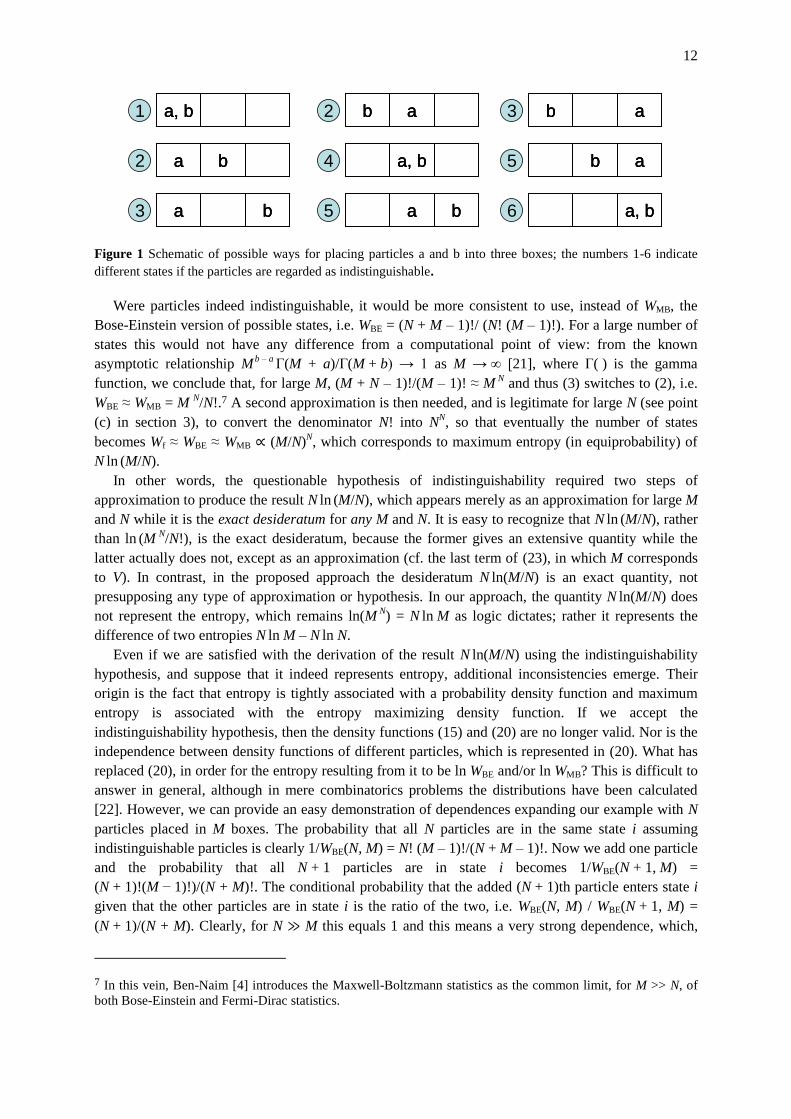
The question is then raised, what does WMB = M N/N! in the Maxwell-Boltzmann statistics really
represent? The answer is illustrated in Figure 1 for the case of N = 2 particles, labelled as a and b,
which are placed into M = 3 boxes. There are W = M N
= 9 possible arrangements. If we regard the
particles as indistinguishable, then the number of possible arrangements is reduced to 6, numbered
from 1 to 6 in Figure 1, where each of numbers 1, 4 and 6 appears once and each of numbers 2, 3 and
5 appear twice. The number 6 is predicted by the Bose-Einstein statistics, i.e. WBE = (N + M – 1)! /
[N! (M – 1)!)] = 4!/(2! 2!) = 6. Now, the number 1/WMB = N!/M N
= 2/9 is, clearly, the probability of
each of the cases 2, 3 and 5. In contrast, each of the cases 1, 4 and 6 has probability 1!/M N = 1/9, so
that all 6 cases indeed sum up to probability 1. We can then observe that the consideration behind
calculating these probabilities does not correspond to maximum entropy, as the possible events are not
equiprobable. Furthermore, the fact that these probabilities are calculated with a denominator M N
indicates that, in fact, the particles are not regarded indistinguishable6; if they were, then the
denominator should be 6, and if entropy was maximized for these 6 cases, then the numerator would
be 1. Thus the number WMB = M N
/N! in (2) seems like a computational trick rather than a result of
consistent analyses based on reasonable hypotheses.
6 In this vein, Papoulis [5] regards the Maxwell-Boltzmann statistics associated with distinguishable particles, in
contrast to statistical thermodynamics texts, such as those cited here, which associate it with indistinguishable
particles.
12
Figure 1 Schematic of possible ways for placing particles a and b into three boxes; the numbers 1-6 indicate
different states if the particles are regarded as indistinguishable.
Were particles indeed indistinguishable, it would be more consistent to use, instead of WMB, the
Bose-Einstein version of possible states, i.e. WBE = (N + M – 1)!/ (N! (M – 1)!). For a large number of
states this would not have any difference from a computational point of view: from the known
asymptotic relationship M b – a Γ(M + a)/Γ(M + b) → 1 as M → ∞ [21], where Γ( ) is the gamma
function, we conclude that, for large M, (M + N – 1)!/(M – 1)! ≈ M N
and thus (3) switches to (2), i.e.
WBE ≈ WMB = M N/N!.7 A second approximation is then needed, and is legitimate for large N (see point
(c) in section 3), to convert the denominator N! into NN, so that eventually the number of states
becomes Wf ≈ WBE ≈ WMB ∝ (M/N)N, which corresponds to maximum entropy (in equiprobability) of
N ln
(M/N).
In other words, the questionable hypothesis of indistinguishability required two steps of
approximation to produce the result N ln
(M/N), which appears merely as an approximation for large M
and N while it is the exact desideratum for any M and N. It is easy to recognize that N ln
(M/N), rather
than ln (M
N/N!), is the exact desideratum, because the former gives an extensive quantity while the
latter actually does not, except as an approximation (cf. the last term of (23), in which M corresponds
to V). In contrast, in the proposed approach the desideratum N ln(M/N) is an exact quantity, not
presupposing any type of approximation or hypothesis. In our approach, the quantity N ln(M/N) does
not represent the entropy, which remains ln(M N
) = N ln M as logic dictates; rather it represents the
difference of two entropies N ln M – N
ln N.
Even if we are satisfied with the derivation of the result N ln(M/N) using the indistinguishability
hypothesis, and suppose that it indeed represents entropy, additional inconsistencies emerge. Their
origin is the fact that entropy is tightly associated with a probability density function and maximum
entropy is associated with the entropy maximizing density function. If we accept the
indistinguishability hypothesis, then the density functions (15) and (20) are no longer valid. Nor is the
independence between density functions of different particles, which is represented in (20). What has
replaced (20), in order for the entropy resulting from it to be ln WBE and/or ln WMB? This is difficult to
answer in general, although in mere combinatorics problems the distributions have been calculated
[22]. However, we can provide an easy demonstration of dependences expanding our example with N
particles placed in M boxes. The probability that all N particles are in the same state i assuming
indistinguishable particles is clearly 1/WBE(N, M) = N! (M – 1)!/(N + M – 1)!. Now we add one particle
and the probability that all N + 1 particles are in state i becomes 1/WBE(N + 1, M) =
(N + 1)!(M − 1)!)/(N + M)!. The conditional probability that the added (N + 1)th particle enters state i
given that the other particles are in state i is the ratio of the two, i.e. WBE(N, M) / WBE(N + 1, M) =
(N + 1)/(N + M). Clearly, for N ≫ M this equals 1 and this means a very strong dependence, which,
7 In this vein, Ben-Naim [4] introduces the Maxwell-Boltzmann statistics as the common limit, for M >> N, of
both Bose-Einstein and Fermi-Dirac statistics.
a, b
a b
a b
a, ba, b
a ba b
a ba b
b a
a, b
a b
b ab a
a, ba, b
a ba b
b a
b a
a, b
b ab a
b ab a
a, ba, b
1
2
3
2
4
5
3
5
6
13
while it is not mathematically impossible, it is physically quite implausible, considering locations of
gas molecules in a container (although it is relevant in other cases involving interacting particles, e.g.
Bose-Einstein condensation). In contrast, in our proposed approach, this conditional probability is
M N
/M N + 1
= 1/M, i.e. independent on N, as reasonably expected for a classical gas in a container.
One may argue that for classical particles in a container the number of particles is always smaller
than the number of possible states, which is infinite, and thus the condition N ≫ M cannot hold.
However, this argument can be refuted by recalling that the entropic mathematical framework is not
necessarily (and only) about the characteristic microscopic states of the particles (also known as
elementary events in probability theory). One can define the entropy for macroscopic states, which
correspond to collections of many, even uncountably many, microscopic states. The ability to make a
description of a system in terms of a partition (a number of mutually exclusive subsets of Ω whose
union equals Ω, where each of the subsets can contain many elementary events), else known as a
coarse grained description, is essential in the entopic framework [5]. Actually, partitioning is tightly
associated with including postulate (d) in the introduction of the entropy function, as described in
section 2; mathematically, this postulate is expressed in terms of a relationship in a partition
refinement [2, p. 3; 18, theorem 1]. As an example, we can coarse grain the description of the
container of particles in motion by defining a partition with only three elements, namely {A1, A2, A3},
with A1 = {z ∈ Ω: 0 ≤ x1 < a/3}, A2 = {z ∈ Ω: a/3 ≤ x1 < 2a/3}, A3 = {z ∈ Ω: 2a/3 ≤ x1 ≤ 1}, where x and
z have been defined in section 3 and a is the length of the container (notice that this partition is defined
considering just one of the coordinates of z, namely x1). In this case, A1 represents a composite event
that a particle is found at the leftmost third of the container, irrespective of the other coordinates and
its velocity. It does not represent a unique characteristic state of a particle (an elementary event) but,
rather it represents a collection of uncountably many events or states, arbitrarily assigned as a
(composite) event by us and thus not representing a characteristic property of the particle per se. The
entropic framework should be valid for this description too, in which M = 3, just as in the example of
Figure 1. In this case, the condition N ≫ M holds true and thus the inconsistency resulting from the
indistinguishability hypothesis is very relevant.
A common justification of the indistinguishability hypothesis has been that there is no way to label
the microscopic particles in a gas and thus they cannot be distinguished from each other. This is
generally correct but irrelevant: Labelling cannot affect the statistical properties and distribution. The
example of Figure 1 can again help us to see that the argument is pointless. In the figure we have
labelled the particles as a and b, and using either the principle of insufficient reason, or the principle of
maximum entropy, we can conclude that, for example, the state where both particles are placed in the
leftmost box is 1/9. We can experimentally test this theoretical result by repeating an experiment many
times, measuring how many times both particles are found in the leftmost box. Now let us erase the
labels and repeat the experiment. Note that the event that both particles are in the leftmost box does
not depend on labels and nothing relating to it will change when we erase the labels. Is it reasonable to
expect that its probability has increased to 1/6, because we erased the labels? We can imagine that a
supporter of the indistinguishability hypothesis would insist that the setting of the above thought
experiment is inappropriate for the microscopic world, in which labelling is not possible at all. But we
can refine the thought experiment to make it more relevant to the microscopic world, assuming two
particles moving in a chamber. Each of them is an atom of each of the two stable isotopes of helium,
so that we can have the possibility to label them by mass number (a = 3He, b =
4He) if we wish. In this
case perhaps we can all agree on the expectation that both atoms will be found in the leftmost third of
the chamber in 1/9 of the time. Now let us remove labelling, or replace the 3He atom with a
4He one to
make labelling impossible. Is it reasonable to expect that now we will find both particles in the
leftmost third of the chamber in 1/6 of the time? There is no doubt that in quantum systems of
interacting particles with a finite number of allowed characteristic states, the question can have a
14
positive answer. However, as explained above, in our classical description of non-interacting
particles, the leftmost third of the chamber does not represent a unique characteristic state of the
particles (an elementary event) but, rather, it represents a collection of uncountably many states (a
composite macroscopic event). Therefore a negative answer of the question is more plausible.
Verification of the negative answer is readily provided by computer simulations of classical systems of
gas particles. As aptly observed by Swendsen [7], if indistinguishability was relevant for this case, it
would require the correction of results obtained from simulating a system of distinguishable particles,
given that computer simulations inevitably use systems of distinguishable particles. A very useful and
enlightening computer application can be found in http://stp.clarku.edu/simulations
/approachtoequilibrium/box/index.html (see also [23]). For example, by setting N = 2, and running the
program for, say, 1000 time steps, we may see that in about 250 (= 1000/4) of them, and not in 333 (=
1000/3), both particles are found in the leftmost half of the box.
8. The Gibbs paradox
We consider two identical parts of a box separated by a diaphragm, each containing N identical
particles with energy E in a volume V. The entropy in each part is Φ(E, V, N). Since independence
between the two parts can be assumed, the total entropy is 2 Φ(E, V, N). If we remove the diaphragm,
the entropy clearly becomes Φ(2E, 2V, 2N) and according to (26) with α = 2, there is an increase of
entropy equal to 2N ln 2. The same result is obtained from (31) by replacing NA and NB with N (and N
with 2N). If we reinsert the diaphragm the entropy will become again 2 Φ(E, V, N) and there will be a
decrease of entropy, –2 N ln 2. These have been regarded as contradictions to thermodynamics, known
as the Gibbs paradox [8,24].
However, according to the probabilistic definition of entropy Φ and its interpretation as a measure
of uncertainty, there is no contradiction or paradox. The increase of entropy after removal of the
diaphragm, quantifies the fact that we have greater uncertainty about the location of each particle.
Initially, we knew each particle’s location with “precision” V and after the removal we lost
information, with the “precision” becoming 2V. The increase of entropy by 2N ln 2, objectively
expresses the lost information, and reflects the physical fact that the motion of each particle has a
bigger domain. Likewise, the decrease of entropy after reinsertion of the diaphragm (which cannot be
thought of as a spontaneous natural phenomenon) reflects the gain of information and the decreased
uncertainty about the position of a particle.
One may contend that the introduction of the diaphragm gives us no information at all about which
part any particular particle might be found in. Such an argument is interesting and in fact can be fully
addressed by the proposed probabilistic approach. Specifically, if we do not know whether a particle is
in one or the other part, then the entropy of the particle is φ as given in (30) and has not been affected
by the diaphragm. However, once the diaphragm is there and once we know that at some time the
particle is in a specific part, then the entropy of the particle has been reduced to φA < φ (the leftmost
term in (30)). The information that the specific particle is in the specific part at a specific time is
important because it is transferred to subsequent times. That is, if we know the part in which a particle
is and there is a diaphragm, then the entropy is φA now and in the future. In contrast, if the diaphragm
is absent, then knowing which part the particle is in makes the entropy φA now, but soon after in the
future this information is lost and the entropy becomes φ. Thus the introduction of the diaphragm is
associated with reduction of uncertainty.
All in all, with the proposed probabilistic framework there is no paradox at all. It is important to see
that the standardized (extensive) entropy Φ* does not change at all when the diaphragm is removed or
reinserted, which indicates full consistence with classical thermodynamics. (It is recalled that the
classical thermodynamic entropy S is identical to Φ*k rather than to Φk).
15
According to the proposed approach, this situation does not change if on either side of the
diaphragm the gases are different, thus removing the asymmetry (or discontinuity) in the two cases
where in the two boxes the gases are different or the same. Again the entropy Φ after the mixing (by
removal of the diaphragm) will be by 2N ln 2 greater than the sum of the entropies in the initial state.
And again, if we consider the mixture of gases as an equivalent single gas (as is the standard practice,
for instance, in the atmospheric mixture) the entropy Φ* will not change, in comparison to the initial
state. The latter is consistent with Ben-Naim’s [4] formulation, “Mixing, as well as demixing, are
something we see but that something has no effect on the MI of the system”, where MI (Missing
Information) actually corresponds to Φ* of our approach, as Ben-Naim uses the indistinguishability
hypothesis. However, since “we see” mixing, there must be an explanation why it happens, and this is
the increased entropy Φ.
9. Summary and concluding remarks
The established idea that, in the microscopic world, particles are indistinguishable and
interchangeable, when used within a classical physical (rather than quantum mechanical) framework,
proves to be problematic on logical and technical grounds. Abandoning this hypothesis does not create
problems but, rather, it helps avoid paradoxical results, such as the Gibbs paradox, associated with a
discontinuity of entropy in mixing gases with different or same particles. More importantly, it avoids a
discontinuity in logic when moving from the microscopic to the macroscopic world, while retaining a
classical framework of description. Such discontinuity cannot stand, as demonstrated by Swendsen
[7,8] using the example of colloids whose particles are large enough to obey classical mechanics and
cannot be regarded indistinguishable. There is no reason why the definition and expression of entropy
in colloids should not be the same as in typical thermodynamic systems, such as ideal gases.
The alternative framework proposed here is the application of the typical probabilistic entropy
definition to thermodynamic systems, such as an ideal gas, treating the particles’ positions and
velocities as random variables, with each particle assigned its own vector of random variables (thus
not using the indistinguishability hypothesis). The entropy calculated in this manner is no longer
extensive. This is not a problem, though. In fact, careful consideration of the probabilistic notion of
entropy reveals that the probabilistic entropy of a system composed of several parts that interact is not
the sum of the entropies of the parts, but includes an additional term, which is the entropy of the
partitioning (related to the probability distribution of a particle being in each part). Furthermore, it is
shown that we can easily adapt the probabilistic entropy to obtain an extensive quantity, which proves
to be identical with the extensive entropy used in classical thermodynamics. This extensive quantity is
the difference of two probabilistic entropies. The rationale in introducing it is to derive a quantity that
is invariant under the observer’s selection of the reference volume for the studied system. It is also
shown that the descriptions of a system by either the typical probabilistic entropy or the extensive
entropy are equivalent, but the quantity that naturally obeys the principle of maximum entropy is the
probabilistic entropy. This provides an explanation for the spontaneous occurrence of mixing, in
which the probabilistic entropy increases while the extensive entropy remains constant.
Is there any usefulness in replacing the typical interpretation of entropy, which includes the
indistinguishability hypothesis, with the proposed framework? A possible reply is that the proposed
interpretation enables potential generalization, rendering the typical formulation of the Second Law a
special case of the more general principle of maximum entropy. Formulating the entropy in pure
probabilistic terms, associating entropy with the notion of a random variable, and interpreting entropy
as none other than uncertainty, makes the same framework applicable in any uncertain system
described by random variables. Removing the barrier between the microscopic and the macroscopic
world, whenever classical descriptions are used in both, enables generalization of mathematical
16
descriptions of processes across any type and scale of systems ruled by uncertainty. Such
generalization is strongly needed in an era dominated by a delusion of the feasibility of deterministic
descriptions of complex systems and a quest for radical reduction of uncertainty, which may be
paralleled to a quest for a perpetual motion machine of the second kind (defined e.g. in ref. [25]). For
example, such generalization on a high level of macroscopization may help explain the marginal
distributional properties of hydrometeorological processes [26], the clustering of rainfall occurrence
[27] and the emergence of Hurst-Kolmogorov dynamics in geophysical and other processes [13, 28].
Acknowledgments The anonymous reviewers’ comments on an earlier version of the paper helped me
to improve the presentation, make the arguments more coherent and avoid some mistaken statements
of the original version. Equally helpful were the comments of an anonymous reviewer of a subsequent
version of the paper, whom I also thank for spotting some errors and for calling my attention to Refs.
[6, 9, 10 and 11]. The discussions with CJ and LM, and particularly their different views, helped me a
lot. I also thank Amilcare Porporato for his interest to read the paper, his detailed corrections and his
encouraging comments. Finally, I am grateful to the Editor Jos Uffink, who despite the rejection of the
original version of the paper (submitted in Jan. 2012) approved my request to resubmit a revision and
thus gave the paper a second chance, whose outcome was positive.
Appendix: Proof of equations (30)-(32)
To show that (30) holds true (cf. also Papoulis, 1991, p. 544) we observe that the unconditional
density f(z) is related to the conditional ones f(z|A) and f(z|B) by
f(z) = π f(z|A)‚ z in A
(1 – π) f(z|B)‚ z in B (33)
Denoting ∫A g(z) dz and ∫B g(z) dz the integral of a function g(z) over the intersection of the domain of z
with the volume A and volume B, respectively, the unconditional entropy will be
φ = Φ[z] = –∫A f(z) ln(f(z)/h(z))dz – ∫B f(z) ln(f(z)/h(z))dz =
= –∫A π f(z|A) ln(π f(z|A)/h(z))dz – ∫B (1 – π) f(z|B) ln((1 – π) f(z|B)/h(z))dz =
= –π ∫A f(z|A) ln(f(z|A)/h(z))dz – π ln π ∫A f(z|A)dz
– (1 – π) ∫B f(z|B) ln(f(z|B)/h(z))dz – (1 – π) ln(1 – π) ∫B f(z|B)dz
We observe that ∫A f(z|A) ln(f(z|A)/h(z))dz = φA and ∫B f(z|B) ln(f(z|B)/h(z))dz = φB, whereas ∫A f(z|A) dz
= ∫B f(z|B) dz = 1. Evidently, then, (30) follows directly.
Further, from (30) we get
φ = (NA/N) φA + (NB/N) φB – (NA/N) ln (NA/N) – (NB/N) ln (NB/N)
Nφ = NA φA + NB φB – NA ln NA – NB ln NB + N ln N
so that (31) follows directly. In turn, from (31) we obtain
φ – ln N = (NA/N) (φA – ln NA) + (NB/N) (φB – ln NB)
Nφ* = NAφ
*A + NB φ
*B
from which (32) follows directly.
References
[1] G. H.Wannier, Statistical Physics, Dover, New York, 532 pp., 1987.
[2] H. S. Robertson, Statistical Thermophysics, Prentice Hall, Englewood Cliffs, NJ, 582 pp., 1993.
[3] K. Stowe, Thermodynamics and Statistical Mechanics (2nd edn., Cambridge Univ. Press, Cambridge, 556 pp.
17
2007.
[4] A. Ben-Naim, A Farewell to Entropy: Statistical Thermodynamics Based on Information, World Scientific Pub.
Singapore, 384 pp., 2008.
[5] A. Papoulis, Probability, Random Variables and Stochastic Processes, 3rd edn., McGraw-Hill, New York, 1991.
[6] N. G. van Kampen, The Gibbs paradox, in Essays in Theoretical Physics, ed. by W. E. Parry, 303-312,
Pergamon, New York, 1984.
[7] R. H. Swendsen, Statistical mechanics of classical systems with distinguishable particles, Journal of Statistical
Physics, 107 (5/6), 1143-1166, 2002.
[8] R. H. Swendsen, Gibbs’ paradox and the definition of entropy, Entropy, 10 (1), 15-18, 2008.
[9] C.-H. Cheng, Thermodynamics of the system of distinguishable particles, Entropy, 11, 326-333, 2009.
[10] M. A. M. Versteegh and D. Dieks, The Gibbs paradox and the distinguishability of identical particles, Am. J.
Phys., 79, 741-746, 2011.
[11] D. S. Corti, Comment on “The Gibbs paradox and the distinguishability of identical particles,” by M. A. M.
Versteegh and D. Dieks, Am. J. Phys., 80, 170-173, 2012.
[12] C. E. Shannon, The mathematical theory of communication, Bell System Technical Journal, 27 (3), 379–423,
1948.
[13] D. Koutsoyiannis, Hurst-Kolmogorov dynamics as a result of extremal entropy production, Physica A, 390 (8),
1424–1432, 2011.
[14] R. H. Swendsen, How physicists disagree on the meaning of entropy, Am. J. Phys., 79 (4), 342-348, 2011.
[15] P. Atkins, Four Laws that Drive the Universe, Oxford Univ. Press, Oxford, 131 pp., 2007.
[16] E. T. Jaynes, Information theory and statistical mechanics, Physical Review, 106 (4), 620-630, 1957.
[17] E. T. Jaynes, Probability Theory: The Logic of Science, Cambridge Univ. Press, Cambridge, 728 pp., 2003.
[18] J. Uffink, Can the maximum entropy principle be explained as a consistency requirement?, Studies In History
and Philosophy of Modern Physics, 26 (3), 223-261, 1995.
[19] E. H. Lieb & J. Yngvason, The entropy of classical thermodynamics, in Entropy, ed. by A. Greven et al.
Princeton Univ. Press, Princeton, NJ, USA, 2003.
[20] C. Tsallis, Entropy, in Encyclopedia of Complexity and Systems Science, ed. by R.A. Meyers, Springer, Berlin,
2009.
[21] M. Abramowitz & I. Stegun, Handbook of Mathematical Functions (10th ed.), 1046 pp., US Government
Printing Office, Washington DC, USA, 1972.
[22] R. K. Niven, Origins of the combinatorial basis of entropy, Bayesian Inference and Maximum Entropy Methods
in Science And Engineering: 27th International Workshop on Bayesian Inference and Maximum Entropy
Methods in Science and Engineering, doi:10.1063/1.2821255, 954, 133-142, 2007.
[23] H. Gould and J. Tobochnik, Statistical and Thermal Physics With Computer Applications, Princeton University
Press, 511 pp., 2010.
[24] E. T. Jaynes, The Gibbs paradox, Maximum entropy and Bayesian methods: proceedings of the Eleventh
International Workshop on Maximum Entropy and Bayesian Methods of Statistical Analysis (Seattle, 1991), 1-
21, Kluwer, Dordrecht, 1992.
[25] D. Kondepudi & I. Prigogine, Modern Thermodynamics, From Heat Engines to Dissipative Structures, Wiley,
Chichester, 1998.
[26] D. Koutsoyiannis, Uncertainty, entropy, scaling and hydrological stochastics, 1, Marginal distributional
properties of hydrological processes and state scaling, Hydrol. Sci. J., 50 (3), 381–404, 2005.
[27] D. Koutsoyiannis, An entropic-stochastic representation of rainfall intermittency: The origin of clustering and
persistence, Water Resour. Res., 42 (1), W01401, doi: 10.1029/2005WR004175, 2006.
[28] D. Koutsoyiannis, A hymn to entropy (Invited talk), IUGG 2011, Melbourne, International Union of Geodesy
and Geophysics, 2011 (http://itia.ntua.gr/1136/).
Recommended