Patent Oppositions∗
Jonathan Levin
Stanford University
Richard Levin
Yale University
August 2002
Abstract
In recent years, patent protection has extended into new areas, giving
rise to serious concern about the lack of clear guidelines for patentability.
We analyze the effect of introducing a patent opposition process that would
allow patent validity to be challenged directly after a patent is granted. In
many cases, such a system would avoid costly litigation at a later date.
In other cases, the opposition process would increase the cost of conflict
resolution, but would also reward holders of valid patents and limit the
rewards to invalid patents. Our analysis suggests significant positive welfare
gains from the introduction of a patent opposition process.
∗We are indebted to the members and staff of the Intellectual Property committee of the
National Academy of Science’s board on Science, Technology and Economic Policy for stimulating
our thinking on this topic. We also thank Barry Nalebuff and Brian Wright for helpful comments.
Email: [email protected] and [email protected].
1 Introduction
In just over two decades, a succession of legislative and executive actions has
served to strengthen substantially the rights of patent holders.1 At the same
time, the number of patents issued in the United States has nearly tripled from
66,290 in 1980 to 184,172 in 2001. Although the surge in patenting has been
widely distributed across technologies and industries, decisions by the Patent and
Trademark Office and the courts have expanded patent rights into three important
areas of technology where previously the patentability of innovations had been
presumed dubious: genetics, software, and business methods.2 As in other areas
of innovation, patents in these fields must meet standards of usefulness, novelty
and non-obviousness. A serious concern, however, in newly emerging areas of
technology is that patent examiners may lack the expertise to assess the novelty
or non-obviousness of inventions, leading to a large number of patents likely to be
invalidated on closer scrutiny by the courts.
Although similar examples could be drawn from the early years of biotechnology
and software patenting, economists in particular will appreciate that many recently
granted patents on business methods fail to meet a common sense test for novelty
and nonobviousness. Presumably, this occurs because the relevant prior art is
unfamiliar to patent examiners trained in science and engineering. Consider U.S.
Patent No. 5,822,736, which claims as an invention the act of classifying products
in terms of their price sensitivities and charging higher mark-ups for those with low
price sensitivity, rather than a constant markup for all products. The prior art most
relevant to judging the novelty of this application is neither documented in earlier
patents nor found in the scientific and technical literature normally consulted by
patent examiners. Instead, it is found in textbooks on imperfect competition,
1Notable among these actions are the Bayh-Dole Patent and Trademark Amendments Act of
1980, the creation of the Court of Appeals for the Federal Circuit in 1982, the Hatch-Waxman
Drug Price Competition and Patent Restoration Act of 1984, the Process Patent Amendments
Act of 1988, and the Trade-Related Aspects of Intellectual Property Rights (TRIPS) Agreement
of 1994.2Three landmark cases regarding, respectively, genetics, software and business methods, are
Diamond v. Chakrabarty, 447 U.S. 303 (1980); Diamond v. Diehr, 450 U.S. 175 (1981); and
State Street Bank & Trust Co. v. Signature Financial Group, Inc. 149 F.3d 1368 (Fed Cir 1998).
1
public utility pricing or optimal taxation.
The almost certain unenforceability of this particular business method patent
may render it of limited economic value, but other debatable patents have al-
ready been employed to exclude potential entrants or extract royalties. A much
publicized example is Jay Walker’s patent (U.S. Patent No. 5,794,207) covering
the price-matching system used by Priceline. After several years of legal wran-
gling, Microsoft Expedia agreed to pay royalties for allegedly infringing on this
patent. Many economists, however, would object that Walker’s patent covers only
a slight variation on procurement mechanisms that have used for hundreds if not
thousands of years. Interestingly, in terms of prior art, Walker’s patent application
cites several previous patents but not a single book or academic article on auctions,
procurement or market exchange mechanisms.
If challenged in court, a patent on the “inverse elasticity rule” would likely be
invalidated for failing to meet the test of novelty or nonobviousness. The Walker
patent, a closer call, also might not survive such scrutiny. But current U.S. law
permits third party challenges only under very limited circumstances. An admin-
istrative procedure, re-examination, is used primarily by patentees to amend their
claims after becoming aware of uncited prior art, but it is also available to third
parties who seek to invalidate a patentee’s claims by identifying prior art, in the
form of an earlier patent or publication, that discloses the precise subject matter
of the claimed invention.3
Broader objections to a patent’s validity can be adjudicated only in response
to a patent holder’s attempts to enforce rights against an alleged infringer. In
response to an infringement suit, the alleged infringer may file a counter-claim
of invalidity. In response to a “desist or pay” letter, the alleged infringer may
seek a declaratory judgment to invalidate the patent. Generally speaking, such
proceedings are very expensive and time consuming. A recent survey estimated
the median cost of a litigated patent infringement suit at $1.5 million in cases
involving stakes of $1 million to $25 million; when the stakes exceed $25 million,
the median cost of a suit was estimated to be $3 million (American Intellectual
3Prior art invalidating the inverse elasticity patent could probably be found. On the other
hand, patents such as Walker’s that are close but not identical to past published ideas typically
cannot be overturned on re-examination.
2
Property Law Association, 2001). A typical infringement suit might take two to
five years from initial filing to final resolution.
What are the costs of uncertainty surrounding patent validity in areas of emerg-
ing technology? First, uncertainty may induce a considerable volume of costly
litigation. Second, in the absence of litigation, the holders of dubious patents
may be unjustly enriched and the entry of competitive products and services that
would enhance consumer welfare may be deterred. Third, uncertainty about what
is patentable in an emerging technology may discourage investment in innovation
and product development until the courts clarify the law, or, in the alternative,
inventors may choose to incur the cost of product development only to abandon the
market years later when their technology is deemed to infringe. In sum, one sus-
pects a timelier and more efficient method of establishing ground rules for patent
validity could benefit innovators, followers, and consumers alike.
One recently suggested remedy is to expand the rights of third parties to chal-
lenge the validity of a patent in a low-cost administrative procedure, before sinking
costly investments in the development of a potentially infringing product, process,
or service (See Merges, 1999, and R. Levin, 2002). Instead of the current re-
examination procedure, which allows post-grant challenges only on very narrow
grounds, the United States might adopt an opposition procedure more akin to
that practiced in Europe, where patents may be challenged on grounds of failing
to meet any of the relevant standards: novelty, nonobviousness, utility, written de-
scription, or enablement. The European system requires only minimal expenditure
by the parties. When interviewed, senior representatives of the European Patent
Office estimated expenditures by each party at less than $100,000. The time re-
quired for adjudication, however, is extremely long, nearly three years, owing to
very generous deadlines for filing of claims, counterclaims, and rebuttals.4
The idea of a streamlined, efficient U.S. administrative procedure for challenges
to patent validity is clearly gaining momentum in the response to mounting concern
about the quality of patents in new technology areas. In its recently released 21st
Century Strategic Plan, the Patent Office stated as one of its intended actions:
“Make patents more reliable by proposing amendments to patent laws to improve
4See Graham, Hall, Harhoff, and Mowery, 2002, for this and other detail on the European
Patent Office’s opposition procedure.
3

a [sic] post-grant review of patents.” (U.S. Patent and Trademark Office, 2002).
This paper makes a modest attempt to evaluate the potential costs and benefits
of introducing such a post-grant opposition process. In the next two sections, we
develop a simple model of patent enforcement and patent oppositions. We model
patent oppositions as essentially a cheaper and earlier way to obtain a ruling on
patent validity. The one further difference between patent opposition and litigation
captured by the model is that patent oppositions can be generated by potential
infringers, while litigation must be initiated or triggered by the patent holder. The
analysis divides naturally into two cases: one where the potentially infringing use
of the patent is rivalrous (i.e. competes directly with the patentee’s product) and
one where the uses are nonrivalrous (i.e. independent or complementary). The
key difference between these cases is that in the former, the patent holder wants
to deter entry while in the latter the patent holder simply wants to negotiate for
a large licensing fee.
We identify several effects of introducing an opposition process. First, if the
parties foresee costly litigation in the absence of an opposition, they have a clear
incentive to use the cheaper opposition process to resolve their dispute. This lowers
legal costs and potentially prevents wasteful expenditure on product development.
At the same time, giving the parties a lower cost method of resolving disputes can
lead to oppositions in cases when the entering firm might either have refrained
from development or been able to negotiate a license without litigation. These
new oppositions have a welfare cost in that the firms incur deadweight costs from
preparing their opposition suits. Nevertheless, these oppositions generate potential
benefits. They can prevent unwarranted patents from resulting in monopoly profits
and, more broadly, if decisions under the opposition process are more informed than
those made directly by the patent examiners, the rewards to patent holders end up
more closely aligned with the true novelty and nonobviousness of their invention.
From a dynamic welfare standpoint, this has the favorable effect of providing more
accurate rewards for innovation.
The model suggests that in some cases, introducing an opposition process will
have an unambiguous welfare benefit, while in other cases there will be a trade-off
between static welfare costs and static and dynamic welfare benefits. In Section
4, we use available information on the cost of litigation and plausible parameters
4
for market size and the cost of development to provide a rough quantitative sense
of the welfare effects. Our general conclusion is that the costs of introducing an
opposition system are likely to be small in relation to the potential benefits.
Section 5 concludes with a discussion of some aspects of the opposition process
not captured in our simple modelling approach. The model provides a reasonable
assessment of how an opposition system affects the gains and losses realized by
a single inventor, a single potential infringer, and their respective customers. It
ignores, however, substantial positive externalities from greater certainty and more
timely information about the likely validity of patents that would flow to other
parties contemplating innovation and entry in a new technology area. In this
respect, our analytic and quantitative findings probably understate the full social
benefit of introducing a low-cost, timely system for challenging patent validity.
2 A Model of Patent Enforcement
We start by developing a simple benchmark model from which we can investigate
the effect of an opposition process. There are two firms. Firm A has a newly
patented innovation, while Firm B would like to develop a product that appears
to infringe on A’s patent. The dilemma is that the legitimacy of A’s patent is
uncertain. In the event of litigation, B may be able to argue convincingly that
part or all of it should be voided.
The interaction between the firms unfolds as follows. Initially Firm B must
decide whether to develop its technology into a viable product. Let k denote the
costs of development. If B does not develop, A will be the monopoly user of its
technology. If B does develop, it can enter negotiations to license A’s technology.
If negotiations are successful, B pays a licensing fee (the precise amount will be
determined by bargaining) and both parties use the technology. If B does not
obtain a license, it may still introduce its product. In this event, A can either
allow B to market its product unhindered or file suit to enforce its intellectual
property rights. If it files suit, the parties enter litigation.
We adopt a simple formulation for thinking about litigation. In litigation,
each party incurs a cost L to prepare its case. At trial, the court assesses the
validity of A’s patent and whether B’s patent infringes upon it. We focus on the
5

determination of validity, since this is the aspect of patent disputes for which an
opposition process has relevance. Let pA and pB denote the subjective probabilities
that Firms A and B assign to the court upholding the patent and let p denote
the true objective probability of validity. We assume that the firms’ subjective
probabilities (but not the true objective probability) are commonly known though
not necessarily equal.5
If the court invalidates the relevant parts of Firm A’s patent, B is free to market
its product. In contrast, if the patent is upheld, A has the option of excluding B
from the market. Firm B may try again to negotiate a license but if it fails A
proceeds to market alone.
The firms’ profits depend on whether B’s product reaches the market and
whether they incur litigation costs. Let πA|B and πA denote the gross profits that
A will realize if B’s product does or does not reach the market. Let πB denote the
gross profits that B’s product will generate. In making decisions, the firms must
factor in these eventual profits as well as development costs, litigation costs and
licensing fees in the event of a licensing agreement.
We model licensing negotiations, both pre-litigation and post-litigation, using
the Nash bargaining solution. This means that if there are perceived gains to
licensing, each party captures its perceived payoff in the absence of a license and
the additional surplus generated by the agreement is divided equally.
The timing of the benchmark model is displayed in Figure 1. After develop-
ment, the firms can negotiate a license. If this fails, B must make a decision about
whether to enter and A can respond by litigating. If there is litigation, the court
rules on the patent’s validity at which point the parties have another opportunity
to negotiate a license.
In thinking about this benchmark situation and the effects of an opposition
5The assumption that pA, pB are commonly known, but not necessarily equal means that
firms will not update beliefs when they negotiate as in standard asymmetric information models.
Rather, they “agree to disagree” about patent validity. This is a simple way to capture the fact
that parties may sometimes end up in court rather than settle. Note that the uncertainty about
patent validity is the only uncertainty in the model – for instance, there is no uncertainty or
learning about whether B’s development will succeed or about the size of the product market.
Accounting for these realistic forms of uncertainty would change the quantitative, but not the
qualitative, conclusions of our model.
6
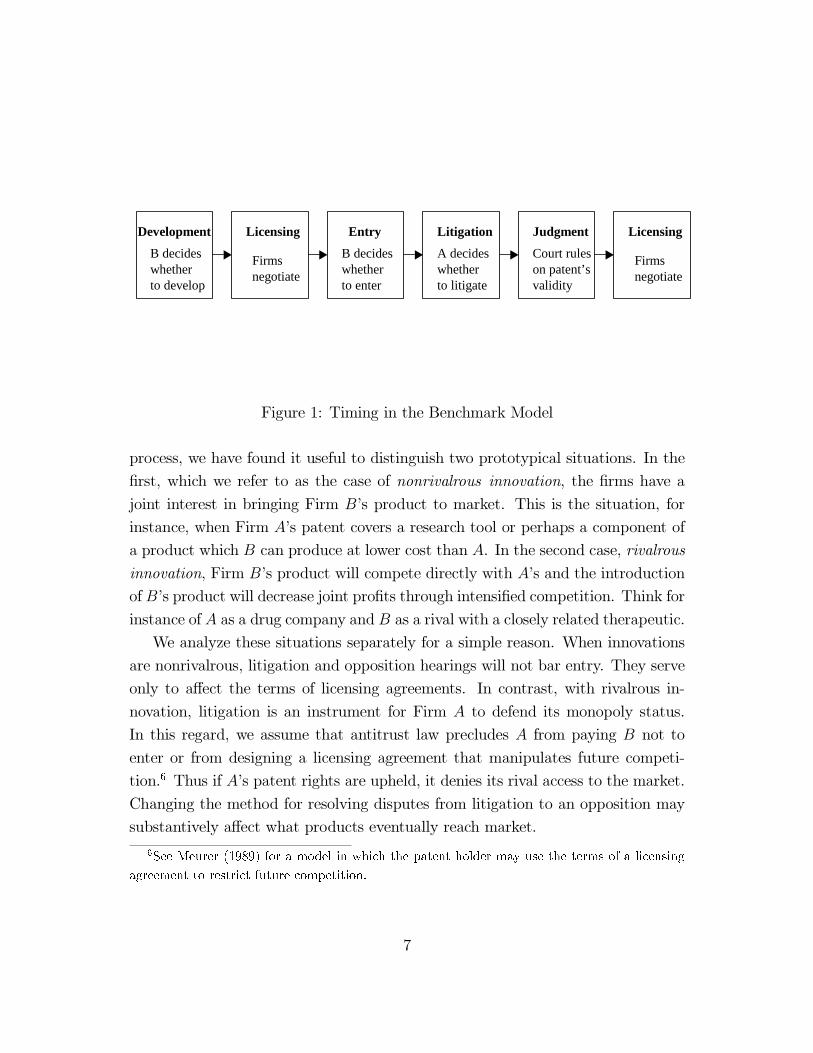
Development Licensing Entry Litigation Judgment Licensing
B decides whetherto develop
Firmsnegotiate
B decideswhetherto enter
A decideswhetherto litigate
Court rules on patent’s validity
Firmsnegotiate
Figure 1: Timing in the Benchmark Model
process, we have found it useful to distinguish two prototypical situations. In the
first, which we refer to as the case of nonrivalrous innovation, the firms have a
joint interest in bringing Firm B’s product to market. This is the situation, for
instance, when Firm A’s patent covers a research tool or perhaps a component of
a product which B can produce at lower cost than A. In the second case, rivalrous
innovation, Firm B’s product will compete directly with A’s and the introduction
ofB’s product will decrease joint profits through intensified competition. Think for
instance of A as a drug company and B as a rival with a closely related therapeutic.
We analyze these situations separately for a simple reason. When innovations
are nonrivalrous, litigation and opposition hearings will not bar entry. They serve
only to affect the terms of licensing agreements. In contrast, with rivalrous in-
novation, litigation is an instrument for Firm A to defend its monopoly status.
In this regard, we assume that antitrust law precludes A from paying B not to
enter or from designing a licensing agreement that manipulates future competi-
tion.6 Thus if A’s patent rights are upheld, it denies its rival access to the market.
Changing the method for resolving disputes from litigation to an opposition may
substantively affect what products eventually reach market.
6See Meurer (1989) for a model in which the patent holder may use the terms of a licensing
agreement to restrict future competition.
7
2.1 Nonrivalrous Innovation
We start by considering nonrivalrous innovation. To focus attention on this case,
we make the following parametric assumption, which is sufficient to ensure that
introducing Firm B’s product generates a joint gain for the two firms.
Assumption NR πA|B + πB − 2k ≥ πA.
In fact, this assumption is slightly stronger than is needed to ensure non-rivalry. A
weaker condition would be that πA|B+πB−k ≥ πA. The stronger condition has the
benefit of guaranteeing that Firm B will have a sufficient incentive to develop prior
to negotiating a license, rather than needing to seek a license prior to development.
Since the effect of an opposition proceeding turns out to be essentially the same
in this latter case, we omit it for the sake of clarity.7
To analyze the model, we work backward. First we describe what happens if
the parties wind up in litigation. We then consider whether litigation will occur
or whether B will negotiate a license or simply enter with impunity. Finally we
consider B’s incentives to develop its product.
Outcomes of Litigation. Suppose that Firm B introduces its product without a
license and Firm A pursues litigation. Two outcomes can result. If the court voids
the relevant sections of A’s patent, B can enter without paying for a license. If
the court upholds A’s patent, B must seek a license. Because the products are
nonrivalrous, there is a gain πA|B+πB−πA > 0 to be realized from an agreement.
Development costs do not appear in the calculation of the gain from introducing
B’s product because they have already been sunk. Nash Bargaining means that
this gain is split equally through a licensing fee FV :
FV =1
2
(πA − πA|B
)+
1
2πB.
Here we use the subscript V to refer to bargaining under the presumption that A’s
patent is valid.
7Note that our definition of non-rivalry does allow Firm A’s profits to decrease if B enters. A
more traditional notion of non-rivalry might require that πA|B ≥ πA. Our more encompassing
definition focuses on joint profitability, which is natural once one realizes that Firm A will be
capture some of Firm B’s profits through licensing fees.
8

Factoring in these two possible outcomes of litigation, we can calculate the
(subjective) expected payoffs to the two firms upon entering litigation. These are
πA|B − L+ pAFV for Firm A and πB − k − L− pBFV for Firm B.
Determinants of Litigation. We now back up and ask what will happen if Firm
B develops its technology.
The first question is whether A has a credible threat to litigate if B attempts
to market its product without a license. Since A’s subjective gains from litigation
are pAFV − L, it will want to pursue litigation only if
pAFV − L ≥ 0. (A)
If this inequality fails, Firm A has a weak patent – the benefit of enforcing it is
smaller than the litigation costs. If A’s patent is weak, Firm B can simply ignore
it and enter without fear or reprisal. Indeed, even if an opposition system is in
place, B would never want to use it since A’s patent is already of no meaningful
consequence. This makes the weak patent case relatively uninteresting from our
perspective. For this reason, we assume from here on that A’s patent is not weak.
Given that Firm A has a credible threat to litigate, we now ask whether litiga-
tion will actually occur. The parties will end up in court if and only if the following
two conditions are met:
πB − pBFV − L ≥ 0 (B)
and
(pA − pB)FV − 2L ≥ 0. (L)
The first condition says that Firm B would prefer to endure litigation than
withdraw its product. The second condition says that the two firms have a joint
incentive to resolve the patent’s validity in court rather than reach a licensing
agreement with validity unresolved. Note that this can only occur if the parties
disagree about the probable outcome in court (i.e. if pA � pB). Moreover, it is
more likely to occur if litigation costs are small relative to the value generated by
B’s product.
If either condition (B) or condition (L) fails, litigation will not occur. Rather
the parties will negotiate a license without resolving the patent’s validity. The
specific license fee is determined by Nash Bargaining with the parties splitting the
9

surplus above their threat points should negotiations fail. If (B) fails, Firm B does
not have a credible threat to litigate so Nash Bargaining results in a licensing fee
FV – in essence, the parties treat the patent as if it were valid. In contrast, if
Firm B has a credible threat to litigate but there is no joint gain to licensing after
litigating (i.e. (L) fails), the alternative to licensing is litigation. In this case, B
will pay a somewhat lower fee FU :
FU =1
2(pA + pB)FV .
Here, the subscript U refers to bargaining under uncertainty about the validity of
the patent. Intuitively, the licensing fee is lower when there is uncertainty about
the patent’s validity.
Development. The last piece of the model is to show that Firm B has an incentive
to develop its product regardless of whether it anticipates licensing or litigation.
The worst outcome for B is that (B) fails and it is forced to pay a licensing cost
FV . Even in this case, however,
πB − k − FV =1
2
(πA|B + πB − πA
)− k ≥ 0.
So B still has an incentive to develop its product, a conclusion that follows directly
from Assumption NR.
We can now summarize the benchmark outcomes when innovation is nonrival-
rous.
Proposition 1 Suppose innovation is nonrivalrous and that Firm A ’s patent is
not weak. The possible outcomes are:
• (Litigation) If both (B) and (L) hold, Firm B develops its product and there
is litigation to determine patent validity. If the patent is upheld, FirmB pays
FV for a license.
• (Licensing without Litigation) If either (B) or (L) fails, Firm B develops and
negotiates a license. The fee is either FU if (B)holds or FV if not.
The table below summarizes the (objective) payoffs to the two firms in each sce-
nario.
10

A’s profit B’s profit
Litigation πA|B + pFV − L πB − k − pFV − L
Licensing πA|B + {FU , FV } πB − k − {FU , FV }
2.2 Rivalrous Innovation
Next we consider the case of rivalrous innovation. To do this, we assume that
introducing Firm B’s product reduces joint profits. The following assumption is
sufficient to imply this.
Assumption R πA|B + πB/pA + 2L/pA < πA.
As in the previous section, this is slightly stronger than is needed. A weaker
condition that would guarantee rivalry is that πA|B + πB − k < πA. The stronger
condition implies that if FirmB chooses to enter, then not only will Firm A have an
incentive to litigate (ruling out the weak patent case), it will not want to license
just to avoid costly litigation. We rule out this latter situation in an effort to
keep the model as simple as possible. Nevertheless, it can be worked out and in
such a circumstance the effect of an opposition process corresponds closely to the
nonrivalrous environment described above.8
To analyze the possible outcomes, we again work backward. We first consider
what would happen in the event of litigation, then ask whether litigation will occur
if B develops, and finally consider the incentive to develop.
Outcomes of Litigation. If Firm B introduces its product and there is litigation,
there are two possible outcomes. If the court voids the patent, B can market
its product without paying any licensing fee. If the court upholds A’s patent,
the rivalry of the products means that A will deny B a license. Thus the firms’
(subjective) profit expectations entering litigation are pAπA+(1− pA)πA|B−L for
Firm A and (1− pB)πB − k − L for Firm B.
8There is also another reason why the firms might want to avoid litigation, which is that
if there are other potential entrants, Firm A may incur a larger cost from having its patent
invalidated than from just allowing B’s entry. We discuss the case of multiple entrants in Section
5.
11

Determinants of Litigation. Now consider what will happen should B develop its
product. If B attempts to introduce its product, Assumption R implies that A
will certainly want to initiate litigation because:
pA(πA − πA|B
)− L ≥ 0. (A)
That is, Assumption R rules out the weak patent case where Firm A is not willing
to defend its intellectual property rights.
At the same time, Firm B is willing to introduce its product and face litigation
if and only if
(1− pB)πB − L ≥ 0. (B)
If this inequality fails, the litigation cost outweighs B’s expected benefit from a
product introduction. If it holds, B will introduce its product and the parties will
end up in court. To see this, we note that under Assumption R, the sum of the
perceived gains from litigation necessarily outweigh the litigation costs so long as
(B) is satisfied. In particular, combining (B) and Assumption R shows that
pA(πA − πA|B
)− pBπB − 2L ≥ 0, (L)
so there is a joint gain to litigation versus a licensing agreement.
Development. Finally we consider Firm B’s incentive to develop. If B would not
introduce a product it developed, it should certainly not develop. On the other
hand, B’s subjective expected profits from litigation are greater than zero if
(1− pB)πB − L− k ≥ 0. (E)
Importantly, whenever (E) holds, so will (B). That is, if B is willing to develop in
expectation of litigation, it certainly wants to litigate having sunk the development
costs. Intuitively, B is more likely to develop and endure litigation if litigation
costs are relatively low, if A’s patent does not seem certain to be upheld, or if the
potential profits from entry are large.
It is now easy to summarize the equilibrium outcomes.
Proposition 2 Suppose that B’s product is rivalrous. The possible outcomes are:
12

• (Litigation) If (E) holds, Firm B will develop its product and there will be
litigation. Firm B will enter if and only if Firm A’s patent is voided.
• (Deterrence) If (E) fails, Firm B is deterred from developing by the threat
of ligation.
The following table summarizes the firm’s expected payoffs in the two cases.
A’s profit B’s profit
Litigation pπA + (1− p)πA|B − L (1− p)πB − k − L
No Entry πA 0
3 An Opposition Process
In this section, we introduce an opposition process that allows for the validity of
A’s patent to be assessed immediately following the granting of the patent. Then,
starting with the benchmark outcomes derived in the previous section, we examine
the effect of allowing for opposition hearings.
With an opposition process, the timing proceeds as follows. Following the grant
of the patent, Firm B is given the opportunity to challenge Firm A’s patent. Prior
to initiating a challenge, B can approach A and attempt to license its technology.
If B does not obtain a license, it must decide whether to challenge. If B declines to
challenge, everything unfolds exactly as in the earlier case – that is, B retains the
option of developing and either licensing or facing litigation. On the other hand,
if B initiates a challenge, the parties enter a formal opposition hearing.
We model the opposition proceeding essentially as a less expensive way of
verifying patent validity than litigation. In an opposition proceeding, each firm
incurs a cost C ≤ L to prepare its case. There are several reasons to believe that
the costs of an opposition would be lower than litigation should the U.S. adopt an
opposition process. First, an opposition hearing would be a relatively streamlined
administrative procedure rather than a judicial process with all the associated cost
of extensive discovery. Second, as noted above, the cost of an opposition in Europe
are estimated by European Patent Office officials to be less than 10% of the cost
of litigation. Although the crossover to the U.S. is imperfect, it suggests that an
13

opposition procedure could be made relatively inexpensive if that were a desired
goal.
Once the parties present their cases in an opposition hearing, an administrator
rules on the patent’s validity. We assume that the firms assign the same subjective
probabilities (pA and pB) to A’s patent being upheld in the opposition process as
in litigation, and also that the objective probability p is the same. Similarly if A’s
patent is upheld in the opposition, Firm B must obtain a license to market its
product. (In particular, Firm A need not endure another round of costly litigation
to enforce its property rights against B.) Conversely if the relevant parts of A’s
patent are voided, B can develop and market its product without fear of reprisal.
3.1 Nonrivalrous Innovation
We now derive the equilibrium outcomes with an opposition process and contrast
these to the benchmark outcomes without an opposition.
The first question is whether Firm B has any incentive to use the opposition
process. If not, the change will have no effect. Assume as before that Firm A’s
patent is not weak (in which case the patent can simply be ignored). Then Firm
B has an incentive to use the opposition process if and only if
πB − k − pBFV − C ≥ ΠB. (BC)
Here ΠB denotes FirmB’s subjective expected payoff should it decline to challenge.
That is, ΠB is the payoff derived for B in the previous section.
If Firm B has a credible threat to use the opposition process, an opposition
proceeding will still only occur if the parties do not have a joint gain from negotiat-
ing a settlement. The sum of their subjective expected payoffs from an opposition
hearing exceeds their joint payoff from licensing if and only if:
(pA − pB)FV − 2C ≥ 0. (C)
Note that this condition is precisely the same as characterizes whether there is a
joint gain from litigation, only the litigation cost L is replaced by the opposition
cost C.
14

If both (BC) and (C) hold, the result is an opposition proceeding. If the patent
is upheld, B will be forced to pay a fee FV for a license. On the other hand if (BC)
holds but (C) does not, there will be licensing under uncertainty at a fee FU .
From here, it is easy to see that the effect of introducing the opposition process
depends on the relevant no-opposition benchmark. If the result without an op-
position process was litigation, then because the incentives to enter an opposition
process are at least as strong as the incentives to enter litigation (since C ≤ L), the
new outcome will be an opposition hearing. Importantly, because an opposition
is less expensive than litigation, both firms benefit from the introduction of the
opposition process.
In contrast, suppose the result without an opposition process would be licensing
at a fee of either FV or FU . In this case, simple calculations show that both
(BC) and (C) may or may not hold. The new outcome depends on the exact
parameters. One possibility with the opposition system in place is that there is no
change. Another possibility is that Firm B goes from not having a credible threat
to fight the patent’s validity in litigation to having a credible threat to launch
an opposition. In this event, the licensing fee drops from FV to FU . The last
possibility is that an opposition proceeding occurs.
What is certain in all these cases is that Firm B’s expected payoff with the
opposition proceeding is at least as high as without it. This should be intuitive.
Introducing the opposition process gives Firm B an option – it can always decline
to challenge and still get its old payoff. On the other hand, A’s expected payoff may
increase or decrease. The case where litigation costs decrease benefits A; the case
where licensing fees decrease hurts A. The case where an opposition proceeding
replaces licensing certainly hurts A if the earlier licensing fee would have been FV ,
but could potentially benefit A if the licensing fee would have been FU .
In the simple static model we are looking at, the direct welfare effects are limited
to the cost of conflict resolution and the change in licensing fees. An important
point however is that the impact on A depends on whether its patent is valid. In
particular, the opposition process tends to help A if its patent is valid and hurt
it if its patent is invalid. Because the opposition process tends to more closely
align the rewards to innovation with truly novel inventions, it seems clear that in a
richer dynamic model where A was to make decisions about R&D expenditures and
15
patent filing, the opposition process would have an additional positive incentive
effect. We argue in Section 4 that this effect might be fairly large in practice
relative to the costs of oppositions.
The next result summarizes oppositions in the nonrivalrous case.
Proposition 3 Suppose products are nonrivalrous and that A’s patent is not
weak. The introduction of a opposition process will have the following effects
depending on the outcome in the benchmark case of no oppositions.
• (Litigation) If the benchmark outcome was litigation, the outcome with an
opposition process will be an opposition. Legal costs are reduced and both
firms benefit.
• (Licensing) If the benchmark outcome was licensing, the outcome with an
opposition process may be the same, or licensing prior to development, or
an opposition. Legal costs may be higher, but license fees will tend to go
down for invalid patents and up for valid patents. The social welfare effects
are ambiguous, because the dead weight loss from the opposition process is
offset by the increased incentive to file valid patents.
3.2 Rivalrous Innovation
We now turn to the case of rivalrous innovation and again consider the effects of
introducing the opposition process.
The first question again is whether Firm B has an incentive to make use of the
opposition procedure. Firm B is willing to initiate an opposition if and only if:
(1− pB)(πB − k)− C ≥ ΠB. (BC)
Again ΠB denotes Firm B’s subjective expected payoff in the absence of opposi-
tions.
Unlike in the nonrivalrous case, (BC) is not just a necessary condition for an
opposition proceeding to occur but also a sufficient condition. If (BC) holds, then
Assumption R implies that the joint benefit from the opposition proceeding exceeds
the costs. In particular, combining (BC) and Assumption R shows that:
pA(πA − πA|B
)− pB(πB − k)− 2C ≥ 0,
16

so there is no gain from licensing rather than facing the opposition process. Thus
if (BC) holds, the new outcome is an opposition, while if it fails the outcome is
unchanged from the no-opposition benchmark.
To see how the opposition process affects previous outcomes, imagine that the
result without an opposition process was litigation. In this case, B was willing
to face litigation for an opportunity to market its product so it will certainly be
willing to ante up the opposition costs. By using the opposition route rather than
the litigation route, B can also avoid sinking the development cost k in the event
that A’s patent is upheld rather than voided. It follows that previous litigation
over the validity of A’s patent will be replaced by opposition hearings.
In contrast, suppose the result without an opposition process was that Firm
B chose not to enter. Now the introduction of oppositions may encourage B to
initiate a challenge. Firm B can enter if the challenge succeeds. From a welfare
standpoint, this potential change has a cost, which is that both firms will have to
spend C on the challenge. It also has the benefit of increased competition. Though
B’s entry will decrease industry profits, the increase in consumer surplus typically
will exceed this loss. Thus the net welfare gain depends on whether the potential
increase in market surplus is greater than 2C.
As in the nonrivalrous case, Firm B always gains from the introduction of the
opposition process. Since it need not use the opposition option, it can certainly do
no worse. Firm A ’s situation is more complex. If it previously would have had to
litigate, it benefits from the cheaper opposition process. If it previously was able
to deter entry without litigation, it loses from having to pay the opposition costs
and loses substantially if its patent, which would not have been litigated, is held
invalid and its monopoly profits disappear.
Proposition 4 Suppose products are rivalrous. Depending on the benchmark
outcome, an opposition system has the following effects:
• (Litigation) If the outcome without oppositions was litigation, the new out-
come is an opposition hearing. This reduces dispute costs and saves on
wasted development costs in the event of a valid patent.
• (Deterrence) If the outcome without oppositions was deterred entry, the new
17

outcome may be an opposition. If it is, dispute costs increase but Firm B is
able to enter if the patent is invalid.
As in the nonrivalrous case, there is a potential dynamic welfare effect in ad-
dition to the static effects. The static welfare effects are limited to the cost of
conflict resolution, the possible reduction in monopoly power and the potential
savings on wasted development. Dynamically, the opposition process also serves
to reward valid patents and punish invalid patents. So again, the better alignment
of rewards with true innovation should tend to provide better incentives for R&D
and patent filing decisions.
4 Welfare Effects of a Opposition Process
Figure 2 summarizes the welfare effects of introducing an opposition system. The
first column distinguishes cases in which Firms A and B are nonrivalrous and
rivalrous. The second column classifies the possible behaviors under a regime
comparable to the current status quo. As the table illustrates, there are four
possible outcomes: litigation and licensing without litigation in the nonrivalrous
case, and litigation and deterrence without litigation in the rivalrous case.
The third column of the table indicates how behavior changes when Firm A’s
patent is subject to challenge in an opposition proceeding. There are now seven
possible outcomes, as described in Section 3 of this paper, and columns four and
five indicate the static welfare and dynamic incentive effects of each outcome.
One striking implication of our model, which is apparent from inspection of
Figure 2, is that once a challenge procedure is available, full-scale litigation never
occurs. This conclusion depends on several of the model’s assumptions concern-
ing full information that are unlikely to represent with accuracy every empirical
situation. For example, some patents are (allegedly) infringed, and thus may be-
come the subject of lawsuits, without the knowledge of the (alleged) infringer, who
may be ignorant that his product, process, or service is potentially covered by the
patent. Or, suppose that both Firms A and B initially agree that the probability
of a patent’s validity is very low. This is the weak patent case that we noted but
did not analyze, in which B’s entry is accommodated by A. In such a circum-
stance, B would not file a challenge, but if, subsequent to B’s entry, A revised its
18

The Welfare Economics of Patent Oppositions
Type of Innovation
Nonrivalrous
Behavior w/o Oppositions Behavior w/ Oppositions Static Wefare Effect Dynamic Wefare Effect
Litigation- license if valid- free entry if invalid
Licensing w/o Litigation
Opposition (1)- license if valid - free entry if invalid
Gain = 2(L-C) Positive
No Change (2)
License at FU not FV (3)
Opposition (4)- license if valid - free entry if invalid
None
None
Loss = 2C
None
Ambiguous
Positive due to sortingof valid/invalid patents.
Rivalrous
Litigation- monopoly if valid- free entry if invalid
Deterrence w/o Litigation
Opposition (5)- monopoly if valid - free entry if invalid
Gain = 2(L-C)+ k if valid
Positive
No Change (6)
Opposition (7)- monopoly if valid - free entry if invalid
None
Loss = 2C; Gain from eliminating monopoly if invalid.
None
Positive due to sortingof valid/invalid patents.
Figure 2: Welfare Effects
19

estimate of validity significantly upward, it might sue for infringement. Finally, an
opposition system would rule only on the validity of A’s patent or specific claims
within the patent. It would not pass judgment on whether a particular aspect of
B’s product infringed on A’s patent. For all these reasons, we clearly would not
expect an opposition system to supplant litigation entirely.
To get a sense of the likely magnitude of the welfare effects displayed in Figure
2, we constructed a simple simulation model, which we calibrated with empirically
plausible parameter estimates. The theoretical model contains nine parameters
(πA, πA|B, πB, pA, pB, p , L, C and k). We add three more in order to make
welfare calculations. The first of these additional parameters is the consumer
surplus generated by the entry of Firm B. The other two represent an attempt
to capture the dynamic incentive effects implicit in an otherwise static model.
Thus, we assume that Firm A’s profits not only enter directly into a social welfare
function that sums consumer and producer surpluses, but that extra weight is
given to A’s profits when it has a valid patent and some weight is subtracted when
it licenses or exclusively exploits an invalid patent.
With so many parameters to vary, a comprehensive presentation of simulation
results would be tedious. Therefore we limit ourselves to describing just two plau-
sible cases, one nonrivalrous and the other rivalrous. In both cases we assume that
the present value of Firm A’s monopoly profit from its patent is $100 million and
that Firm B must spend $20 million to develop its innovation. We also assume that
patent litigation costs each party $2.5 million, which, given the size of the market,
is consistent with the estimates reported by the American Intellectual Property
Law Association. We assume, given the U.S. propensity to spend on lawyers, that
the cost of an opposition proceeding would be 20% of the cost of litigation, or
$500,000 for each party. This is a conservative assumption in light of the report
of the European Patent Office that oppositions cost less than $100,000. Finally, in
both nonrivalrous and rivalrous examples, we assume that the objective probability
of the validity of Firm A’s patent is 0.55, corresponding to the empirical frequency
of validity calculated by Allison and Lemley (1998) on all litigated patent cases
from 1989 through 1996.
In the nonrivalrous case we assume that Firm B’s entry would yield it a gross
profit of $60 million and generate an equivalent amount of consumer surplus. We
20

also assume no decline in Firm A’s gross profit given B’s entry. This leaves us free
to examine what happens as we vary first the subjective probabilities of validity
and then the dynamic welfare parameters. For simplicity, we assume that the
subjective probabilities of A and B are symmetric around the objective probability
of 0.55.
Under these circumstances, if the firms have very similar expectations about
the validity of the patent, there will be no litigation prior to the introduction of a
challenge system and no use of the opposition procedure thereafter. This situation
is represented as Case (2) in Figure 2. The introduction of an opposition system
has no effect on either static or dynamic welfare.
If the expectations of the firms diverge by more than 0.032 but less than 0.166
(i.e., as Firm A’s subjective probability of validity increases from 0.566 to 0.633)
there would be no litigation prior to the introduction of a challenge system, but
Firm B would initiate an opposition proceeding. This situation is represented as
Case (4) in Figure 2. There is a net static welfare loss equal to the total cost of an
opposition proceeding, or $1 million. Still, the opposition process has advantages
because it sorts out valid from invalid patents. If, when the patent is valid, we
give an additional positive weight of only 14% to Firm A’s profit as a proxy for
the incentive effect, then the welfare benefits of an opposition system outweigh the
cost of a proceeding. If we subtract an equal percentage from A’s profit when its
patent is ruled invalid, we need add only an 8% weight to offset the cost of the
opposition proceeding. If we give substantial weight to these incentive effects, such
as counting as a component of social welfare 150% of A’s profit in the case of a
valid patent and only 50% if the patent is invalid, then introducing an opposition
system increases social welfare by $6.4 million.
The final possibility arises when the divergence in subjective probabilities ex-
ceeds 0.166 (i.e., Firm A’s subjective probability exceeds 0.633). In this instance,
there is an unambiguous social benefit of the difference between the total cost of
litigation and the total cost of opposition, as represented in Case (1) in Figure 2.
Given our assumptions, this produces a gain of $4 million. Since our model im-
plies that half the gain is realized by Firm A, there is a small (favorable) dynamic
incentive effect. In this case, however, the gain comes not from sorting valid from
invalid patents, but because Firm A captures a portion of the social saving.
21
To explore the rivalrous case, we vary only two parameters and assume that
the present value of post-entry gross profits of Firms A and B are now $45 million.
Again, if the subjective probabilities of validity are close together, litigation will
not occur, because Firm B’s entry can be deterred without it. In this instance,
if the difference in subjective probabilities does not exceed 0.1 (i.e., Firm A’s
subjective probability does not exceed 0.6), there will be no litigation but B will
challenge A if oppositions are permitted. As shown in Case (7) in Figure 2, there
is a static welfare loss equal to the total cost of the challenge ($1 million) if the
patent is valid. If the patent is not valid, there is a substantial net gain of $29
million, representing the incremental producer plus consumer surplus ($50 million)
created by B’s entry minus the development cost ($20 million) minus the cost of
the challenge ($1 million).
Finally, if Firms A and B have subjective probabilities that differ by more than
0.1, litigation will occur when oppositions are not permitted. If oppositions are
allowed, a challenge will be lodged and, as in Case (5) in Figure 2, there will be
an unambiguous gain in static welfare, amounting to $4 million if the patent is
invalid and $24 million if the patent is valid, because B will not sink the cost of
development if it loses a challenge.
In all, it would appear that the cost of introducing an opposition procedure
is quite small relative to the potential static welfare gains and dynamic incentive
effects. A static welfare loss arises only when a challenge is lodged under circum-
stances that would not have given rise to litigation, such as when the parties do
not differ greatly in their subjective expectations of the patent’s validity. In such
instances the loss is never greater than the cost of both parties participating in
the administrative proceeding, which, if European experience is any guide, is likely
to be modest. By contrast, both the potential static and dynamic welfare gains
that arise under other circumstances will be considerably larger. The low cost
opposition procedure will often supplant higher cost litigation; larger profits to the
innovator will provide a favorable dynamic incentive, and wasteful development
expenses may sometimes be avoided. All of these effects are likely to be larger in
magnitude than the cost of an opposition proceeding.
22
5 Discussion
The analysis of our two firm model of a patentee and potential entrant makes clear
that in this simple framework an opportunity to contest the validity of an issued
patent is likely to yield net social benefits. In the model, however, benefits and
costs are evaluated strictly by the standard welfare metrics in the product markets
occupied by Firms A and B, assuming that there are no additional firms that
might potentially infringe on A’s patent. As a result, the model fails to capture
several additional effects and likely benefits of introducing an opposition system.
First, opposition proceedings should speed the education of patent examiners
in emerging technologies. Third parties will tend to have far greater knowledge of
the prior art in fields that are new to the Patent and Trademark Office. Allowing
the testimony of outside experts to inform the opposition proceedings should have
substantial spillovers in pointing patent examiners to relevant bodies of prior art,
thus making them more likely to recognize non-novel or obvious inventions when
they first encounter them.
Second, in an emerging area of technology, a speedy clarification of what is
patentable and what is not confers substantial external benefit on those who wish
to employ the new technologies. Because precedent matters in litigation and would
presumably matter in opposition proceedings, a decision in one case, to the ex-
tent it articulates principles and gives reasons, has implications for many others.
Clarifying the standard of patentability in an area could have significant effects
on firms developing related technologies, even if these technologies are unlikely to
infringe on the patent being examined. Early decisions making clear the standard
of patentability would encourage prospective inventors to invest in technology that
is appropriable and shun costly investments in technology that might later prove
to be unprotected.
More narrowly, clarifying the validity of a patent has an obvious effect on future
users of the technology.9 In fact, it is not difficult to broaden our two firm model
9See Choi (1998) for a model where there is a single patent holder and several potential
infringers. Choi points out that a free-rider problem may arise in this environment, whereby
a potential infringer on a patent may hesitate to introduce its product in hopes that another
infringer on the same patent will enter first and the ensuing litigation will clarify the patent’s
validity. This kind of free-rider problem could also arise with an opposition process, though it
23

to allow for future infringers on A’s patent. One important change then is that
A’s future profits are likely to depend on whether or not a definitive decision is
handed down concerning the validity of its patent. In principle, this future patent
value effect might make A either more or less inclined to grant an early infringer
a license. To the extent that A becomes more inclined to grant a license, this can
lead to one new outcome not captured in the model – the firms may negotiate a
license even if B’s product is rivalrous. In this case, the introduction of oppositions
can result in a hearing when without the opposition process the result would have
been licensing, with consequent positive and negative welfare effects.
In closing, we note that we have offered little guidance about the specific design
of a system permitting post-grant review of patent validity. To be effective, such
a system should have a broader mandate than the current re-examination process,
which is not an adversary proceeding and which allows third party intervention on
only very limited grounds. Presumably, a more thoroughgoing U.S. system would
allow challenges to validity on any of the familiar grounds now available to litigants
in a court proceeding. The testimony of experts and the opportunity for cross-
examination would seem desirable as a means of probing questions of novelty and
nonobviousness. Still, it would be important to avoid extensive pre-hearing discov-
ery, unlimited pre-hearing motions, and protracted hearings. The costs of using
a challenge system should be kept substantially below that of full-scale infringe-
ment litigation or its benefits will become negligible. In designing an opposition
system, we would do well to examine the diverse experience with administrative
proceedings in various Federal agencies and imitate the best practices.
References
Allison, John and Mark Lemley, “Empirical Evidence on the Validity of Litigated
Patents,” American Intellectual Property Law Association Quarterly Journal,
1998, 26, 185—277.
American Intellectual Property Law Association, Economic Survey, 2001.
would be mitigated to the extent that the cost of oppositions can be kept low.
24

Choi, Jay Pil, “Patent Litigation as an Information Transmission Mechanism,”
American Economic Review, December 1998, 88, 1249-1263.
Graham, Stuart, Bronwyn Hall, Dietmar Harhoff and David Mowery, “Post-
Issue Patent ‘Quality Control’: A Comparative Study of US Patent Re-
Examinations and European Patent Oppositions,” U.C. Berkeley mimeo,
2002.
Levin, Richard, Testimony before the FTC-DOJ Joint Hearings on Competition
and Intellectual Property Law, Washington, D.C., February 6, 2002.
Merges, Richard, “As Many as Six Impossible Patents before Breakfast: Property
Rights for Business Methods and Patent System Reform,” Berkeley Technol-
ogy Law Journal, Spring 1999, 14, 577—616.
Meurer, Michael, “The Settlement of Patent Litigation,” Rand Journal of Eco-
nomics, Spring 1989, 20, 77—91.
U.S. Patent and Trademark Office, The 21st Century Strategic Plan, June 3, 2002.
25
Recommended