The 14th IFToMM World Congress, Taipei, Taiwan, October 25-30, 2015 DOI Number: 10.6567/IFToMM.14TH.WC.OS8.017

Parametrization-Independent Non-Uniform Fourier Approach to

Path Synthesis of Four-Bar Mechanism

Xiangyun Li1 Xu Zhong2 Q. J. Ge3

Southwest Jiaotong University Stony Brook University Stony Brook University

Chengdu, P. R. China Stony Brook, USA Stony Brook, USA

Abstract: This paper deals with the classical problem of

dimensional synthesis of planar four-bar linkages for path

generation. Using Fourier descriptors, a given path is

represented by harmonic series. Extensive research has

been done on this approach in mechanism synthesis with

the assumption that the path is assigned a prescribed

parametrization or timing beforehand, and the input link of

mechanisms rotates with constant angular velocity.

However, little research efforts have been put into pure

path synthesis independent of parametrization. In this

paper, we present an exact method that can efficiently and

accurately carry out the pure path matching using arc

length parametrization. Meanwhile, curve normalization

combined with artificial neural network is used to decouple

the design space, which leads naturally to a fast synthesis

approach. Keywords: Linkage synthesis, Fourier descriptors, Parametrization

I. Introduction

This paper studies the problem of dimensional

synthesis of planar four-bar linkages for path generation

using Fourier descriptors. Central to this problem is the

formulation of an error function that quantifies the

deviation of the generated path from the desired path in

terms of nine independent variables associated with the

design of a four-bar linkage. When the error function

attempts to use all nine variables to compare the shape, size,

location, and orientation of the two paths simultaneously, it

makes the resulting optimization routine highly inefficient.

Synthesis approach that has received increasing

attention lately is the use of Fourier descriptors for linkage

synthesis. This idea was first explored by Freudenstein [1]

in the context of function generation. The research was

followed by Funabashi [2], Farhang et al. [3], [4], Chu and

Cao [5], and McGarva [6], [7], and Ullah and Kota [8], and

Nie and Krovi [9]. Lately, Chu and Sun [10], [11], [12]

have extended Fourier descriptor based method to the

synthesis of spherical and spatial linkages. One of the key

feature of the Fourier descriptor based method is the ability

to decouple the nine design variables involved in path

generation. Ullah and Kota [8] was the first to present this

conclusion and used it to reduce the dimension of the search

space from nine to five. Recently, Wu et al. [13]

further reduced the search dimension from five to four.

1xiangyun.app@gmail.com

2zhongxu2@gmail.com 3qiaode.ge@stonybrook.edu

Another important feature is that while the path of a coupler

point depends on the choice of the coupler point, one may

extract a subset of Fourier descriptors of the path in such a

way that they depend only on the linkage dimensions but

not the choice of the coupler point. This means that for each

four bar linkage, one set of Fourier descriptors can be used

to tag all its coupler curves. Chu and Wang [14] made this

key observation and achieved significant reduction in the

size of the database for numerical atlas. Xie and Chen [15]

was the first to extend Fourier descriptor method to the

image space of kinematic mapping to solve the whole cycle

motion generation problem in four bar linkage synthesis. In

their work, image curve of a desired motion was indexed

with Fourier descriptors (FDs) which were used to be

matched with those of four-bar coupler motion. Neural

networks was used to establish the relationship between

FDs and dimensions of a four-bar linkage.

While the Fourier-based approach has been extensively

used to synthesize mechanism for path and motion

generation, it has its own limitation in such application:

dependency on parametrization or timing. Nie and Krovi [9]

noticed this problem and artfully utilized it to render

smallest number of harmonic components for synthesizing

coupled multi-link serial open chain with smallest number

of links. Vasiliu and Yannou [16] also mentioned para-

metrization issue in their paper but in effect handled the

problem of different samplings under a given para-

metrization, which is a sampling-independent method. In

general, Fourier transform is conducted against timing

parameter t in signal processing. However, problem arises

when it comes to geometry analysis. When processed by

Fourier Transform, different parametric forms of a task

curve would yield different Fourier descriptors. In Fig. 1,

the unit circle is assigned two different parametrizations

𝑧1(𝑡) and 𝑧2(𝑡) . The Fourier transform of 𝑧1(𝑡) is 𝑧1(𝑡)=

𝑒𝑗2π𝑡 while 𝑧2(𝑡) is decomposed as:

𝑧2(𝑡) = (0.1607 + 0.3138i) + (1)

(−0.0759 + 0.0285i) 𝑒−𝑗2π𝑡 + (0.6117 − 0.6020i) 𝑒𝑗2π𝑡 +

(0.0053 − 0.0018i) 𝑒−𝑗4π𝑡 + (0.3111 + 0.1758i) 𝑒𝑗4π𝑡 +

(−0.0045 + 0.0019i) 𝑒−𝑗6π𝑡 + (−0.0090 + 0.0674i) 𝑒𝑗6π𝑡

It is clear that two sets of Fourier descriptors are

completely different from each other, though they both

define the same geometric curve, i.e., the unit circle.

As with task curve, the mechanism coupler curve shares

the same problem. When the crank rotates, a curve would

be traced out by coupler point of the mechanism. For a

mechanism of fixed dimensions, different crank rotation

functions could lead to different parametrization or timing

for the coupler curve. Traditional ways of path synthesis

approaches (see Chu [14] and Wu [17]) assume that crank

always rotates with constant angular velocity and hence

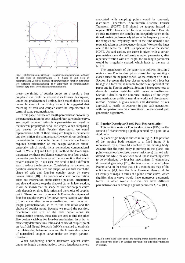
Fig. 1. Solid line: parametrization 1. Dash line: parametrization 2. a) Shape of unit circle in parametrization 1; b) Shape of unit circle in

parametrization 2; c) 𝑥 component of parametrization function 𝑧(t) under

two different parametrizations; d) 𝑦 component of parametrization

function 𝑧(t) under two different parametrizations

preset the timing of coupler curve. As a result, a best

coupler curve could be missed if its Fourier descriptors,

under that predetermined timing, don’t match those of task

curve. In view of the timing issue, it is suggested that

matching of task and coupler curve be implemented in

terms of same parametrization.

In this paper, we use arc length parametrization to unify

the parametrization for both task and four-bar coupler curve.

Arc length parametrization is a parametrization based on

the inherent property of curve: arc length. When comparing

two curves by their Fourier descriptors, we could

reparametrize both of them using arc length as parameter

and then initiate the comparison. However, direct arc length

parametrization for coupler curve of four-bar mechanism

requires determination of ten design variables simul-

taneously, which would incur tremendous computational

cost. In Wu’s [17] and Chu’s [14] method, the ten-design-

parameter synthesis problem is converted to a four-design-

parameter problem because of the assumption that crank

rotates constantly. In our case, we need to find a different

way to reduce the design cost. Considering that a curve has

position, orientation, size and shape, we can first match the

shape of task and four-bar coupler curve by curve

normalization [18]. The process of curve normalization

takes out information about curve’s position, orientation

and size and merely keep the shape of curve. In later section,

it will be shown that the shape of four-bar coupler curve

only depends on three link ratios and the choice of coupler

point. Therefore, we try to match Fourier descriptors of

four-bar coupler curve after curve normalization with that

of task curve after curve normalization, both under arc

length parametrization, so as to find link ratios and the

choice of coupler point. Because we record the position,

orientation and size of the task curve along its

normalization process, those data are used to find the other

five design variables for four-bar mechanism. In order to

efficiently determine link ratios and choice of coupler point,

an Artificial Neural Network (ANN) is trained to establish

the relationship between them and the Fourier descriptors

of normalized coupler curve under arc length parame-

trization.

When conducting Fourier transform against curve

under arc length parametrization, the arc length parameters

associated with sampling points could be unevenly

distributed. Therefore, Non-uniform Discrete Fourier

Transform (NDFT) [19] should be adopted instead of

regular DFT. There are two forms of non-uniform Discrete

Fourier transform: the samples are irregularly taken in the

time domain t but irregularly taken in the frequency domain;

the samples are irregularly taken in the time domain t but

regularly taken in the frequency domain. We take the latter

one in the sense that DFT is a special case of the second

NDFT. As said earlier, the curve is given with a certain

parametrization and a uniformly sampled parameter t; after

reparametrization with arc length, the arc length parameter

would be irregularly spaced, which leads to the use of

NDFT.

The organization of the paper is as follows. Section 2

reviews how Fourier descriptors is used for representing a

closed curve on the plane as well as the concept of NDFT.

Section 3 presents the loop closure equation of a four bar

linkage in a form that is suitable for the development of this

paper and its Fourier analysis. Section 4 introduces how to

decouple design variables with curve normalization.

Section 5 details on the numerical analysis of arc-length

parametrization, artificial neural networks and direct search

method. Section 6 gives results and discussion of our

approach to justify its accuracy in pure path generation,

with comparison against conventional Fourier-based path

generation algorithms.

II. Fourier Descriptor Based Path Representation

This section reviews Fourier descriptors (FDs) in the

context of characterizing a path generated by a point on a

rigid body.

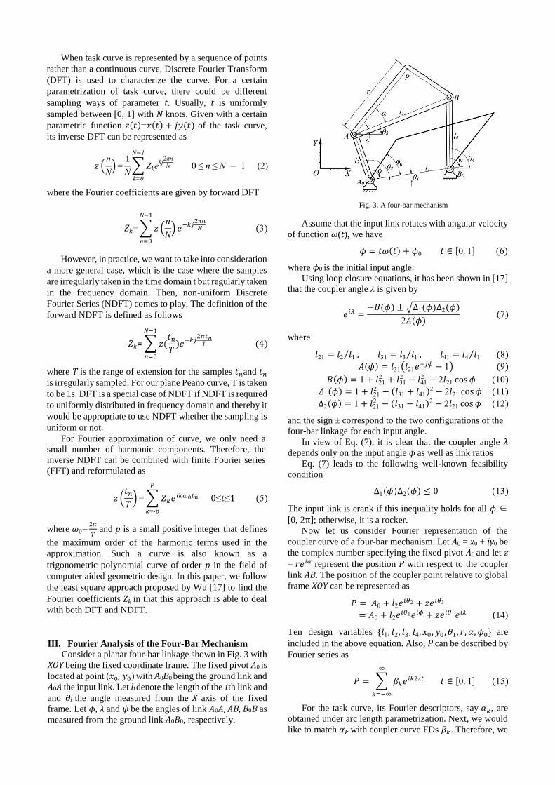
A planar rigid body is shown in in Fig. 2. The position

of the moving body relative to a fixed frame F is

represented by a frame M attached to the moving body.

Assume that the rigid body is moving in the plane, one

point v traces out the closed curve (task curve) marked with

dashed line while the one with solid line is matching curve

to be synthesized by four-bar mechanism. In elementary

differential geometry [20], the task curve is called plane

Peano curve in the sense that it is a continuous map of the

unit interval [0,1] into the plane. However, there could be

an infinity of maps in terms of a plane Peano curve, which

signifies that a curve would have numerous parametric

forms. In other words, a curve can have different

parametrizations or timings against parameter t, t ∈ [0,1].

Fig. 2. F is the fixed frame and M the moving frame. Dashed-line path is

generated by the point v on the rigid body and solid-line path synthesized

by linkage.

When task curve is represented by a sequence of points

rather than a continuous curve, Discrete Fourier Transform

(DFT) is used to characterize the curve. For a certain

parametrization of task curve, there could be different

sampling ways of parameter t. Usually, t is uniformly

sampled between [0, 1] with N knots. Given with a certain

parametric function 𝑧(𝑡)=𝑥(𝑡) + 𝑗𝑦(𝑡) of the task curve,

its inverse DFT can be represented as

𝑧 (n

N) =

1

N∑ Zke

kj2πnN

N−1

k=0

0 ≤ n ≤ N − 1 (2)

where the Fourier coefficients are given by forward DFT

Zk= ∑ 𝑧 (n

N) 𝑒−𝑘𝑗

2π𝑛𝑁 (3)

N−1

n=0

However, in practice, we want to take into consideration

a more general case, which is the case where the samples

are irregularly taken in the time domain t but regularly taken

in the frequency domain. Then, non-uniform Discrete

Fourier Series (NDFT) comes to play. The definition of the

forward NDFT is defined as follows

𝑍k= ∑ 𝑧(𝑡𝑛

𝑇)𝑒−𝑘𝑗

2𝜋𝑡𝑛𝑇

𝑁−1

𝑛=0

(4)

where T is the range of extension for the samples 𝑡𝑛and 𝑡𝑛

is irregularly sampled. For our plane Peano curve, T is taken

to be 1s. DFT is a special case of NDFT if NDFT is required

to uniformly distributed in frequency domain and thereby it

would be appropriate to use NDFT whether the sampling is

uniform or not.

For Fourier approximation of curve, we only need a

small number of harmonic components. Therefore, the

inverse NDFT can be combined with finite Fourier series

(FFT) and reformulated as

𝑧 (𝑡𝑛

𝑇) = ∑ 𝑍𝑘𝑒𝑖𝑘𝜔0𝑡𝑛

𝑝

𝑘=-𝑝

0≤𝑡≤1 (5)

where 𝜔0=2𝜋

𝑇 and p is a small positive integer that defines

the maximum order of the harmonic terms used in the

approximation. Such a curve is also known as a

trigonometric polynomial curve of order p in the field of

computer aided geometric design. In this paper, we follow

the least square approach proposed by Wu [17] to find the

Fourier coefficients Zk in that this approach is able to deal

with both DFT and NDFT.

III. Fourier Analysis of the Four-Bar Mechanism

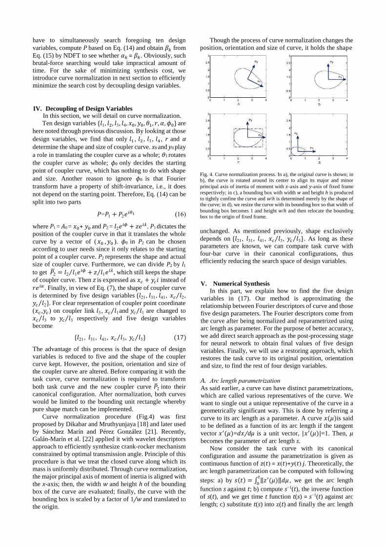
Consider a planar four-bar linkage shown in Fig. 3 with

XOY being the fixed coordinate frame. The fixed pivot A0 is

located at point (𝑥0, 𝑦0) with A0B0 being the ground link and

A0A the input link. Let li denote the length of the 𝑖th link and

and θi the angle measured from the 𝑋 axis of the fixed

frame. Let ϕ, λ and ψ be the angles of link A0A, AB, B0B as

measured from the ground link A0B0, respectively.

Fig. 3. A four-bar mechanism

Assume that the input link rotates with angular velocity

of function ω(t), we have

𝜙 = 𝑡𝜔(𝑡) + 𝜙0 𝑡 ∈ [0, 1] (6)

where ϕ0 is the initial input angle.

Using loop closure equations, it has been shown in [17]

that the coupler angle λ is given by

𝑒𝑖𝜆 =−𝐵(𝜙) ± √Δ1(𝜙)Δ2(𝜙)

2𝐴(𝜙) (7)

where

𝑙21 = 𝑙2 𝑙1⁄ , 𝑙31 = 𝑙3 𝑙1⁄ , 𝑙41 = 𝑙4 𝑙1⁄ (8)

𝐴(𝜙) = 𝑙31(𝑙21𝑒−𝑗𝜙 − 1) (9)

𝐵(𝜙) = 1 + 𝑙212 + 𝑙31

2 − 𝑙412 − 2𝑙21 cos 𝜙 (10)

𝛥1(𝜙) = 1 + 𝑙212 − (𝑙31 + 𝑙41)2 − 2𝑙21 cos 𝜙 (11)

Δ2(𝜙) = 1 + 𝑙212 − (𝑙31 − 𝑙41)2 − 2𝑙21 cos 𝜙 (12)

and the sign ± correspond to the two configurations of the

four-bar linkage for each input angle.

In view of Eq. (7), it is clear that the coupler angle λ depends only on the input angle ϕ as well as link ratios

Eq. (7) leads to the following well-known feasibility

condition

Δ1(𝜙)Δ2(𝜙) ≤ 0 (13)

The input link is crank if this inequality holds for all ϕ ∈

[0, 2π]; otherwise, it is a rocker.

Now let us consider Fourier representation of the

coupler curve of a four-bar mechanism. Let A0 = x0 + iy0 be

the complex number specifying the fixed pivot A0 and let z

= 𝑟𝑒𝑖𝛼 represent the position P with respect to the coupler

link AB. The position of the coupler point relative to global

frame XOY can be represented as

𝑃 = 𝐴0 + 𝑙2𝑒𝑖𝜃2 + 𝑧𝑒𝑖𝜃3

= 𝐴0 + 𝑙2𝑒𝑖𝜃1𝑒𝑖𝜙 + 𝑧𝑒𝑖𝜃1𝑒𝑖𝜆 (14)

Ten design variables {𝑙1, 𝑙2, 𝑙3, 𝑙4, 𝑥0, 𝑦0 , 𝜃1, 𝑟, 𝛼, 𝜙0} are

included in the above equation. Also, P can be described by

Fourier series as

𝑃 = ∑ 𝛽𝑘𝑒𝑖𝑘2π𝑡

∞

𝑘=−∞

𝑡 ∈ [0, 1] (15)

For the task curve, its Fourier descriptors, say 𝛼𝑘, are

obtained under arc length parametrization. Next, we would

like to match 𝛼𝑘 with coupler curve FDs 𝛽𝑘. Therefore, we

have to simultaneously search foregoing ten design

variables, compute P based on Eq. (14) and obtain 𝛽𝑘 from

Eq. (15) by NDFT to see whether 𝛼𝑘 = 𝛽𝑘. Obviously, such

brutal-force searching would take impractical amount of

time. For the sake of minimizing synthesis cost, we

introduce curve normalization in next section to efficiently

minimize the search cost by decoupling design variables.

IV. Decoupling of Design VariablesIn this section, we will detail on curve normalization.

Ten design variables {𝑙1, 𝑙2, 𝑙3, 𝑙4, 𝑥0, 𝑦0, 𝜃1, 𝑟, 𝛼, 𝜙0} are

here noted through previous discussion. By looking at those

design variables, we find that only 𝑙1 , 𝑙2 , 𝑙3 , 𝑙4 , r and α determine the shape and size of coupler curve. x0 and y0 play

a role in translating the coupler curve as a whole; θ1 rotates

the coupler curve as whole; ϕ0 only decides the starting

point of coupler curve, which has nothing to do with shape

and size. Another reason to ignore ϕ0 is that Fourier

transform have a property of shift-invariance, i.e., it does

not depend on the starting point. Therefore, Eq. (14) can be

split into two parts

𝑃=𝑃1 + 𝑃2𝑒𝑖𝜃1 (16)

where P1 = A0 = 𝑥0+ 𝑦0 and P2 = 𝑙2𝑒𝑖𝜙 + 𝑧𝑒𝑖𝜆. P1 dictates the

position of the coupler curve in that it translates the whole

curve by a vector of ( 𝑥0 , 𝑦0 ). ϕ0 in P2 can be chosen

according to user needs since it only relates to the starting

point of a coupler curve. P2 represents the shape and actual

size of coupler curve. Furthermore, we can divide P2 by l1

to get 𝑃2̅ = 𝑙2 𝑙1𝑒𝑖𝜙 + 𝑧 𝑙1𝑒𝑖𝜆⁄⁄ , which still keeps the shape

of coupler curve. Then z is expressed as 𝑥𝑐 + 𝑦𝑐𝑖 instead of

𝑟𝑒𝑖𝛼 . Finally, in view of Eq. (7), the shape of coupler curve

is determined by five design variables {𝑙21, 𝑙31, 𝑙41, 𝑥𝑐 𝑙2,⁄𝑦𝑐 𝑙2⁄ }. For clear representation of coupler point coordinate

(𝑥𝑐 ,𝑦𝑐 ) on coupler link 𝑙3 , 𝑥𝑐 𝑙1⁄ and 𝑦𝑐 𝑙1⁄ are changed to

𝑥𝑐 𝑙3⁄ to 𝑦𝑐 𝑙3⁄ respectively and five design variables

become

{𝑙21, 𝑙31, 𝑙41, 𝑥𝑐 𝑙3, ⁄ 𝑦𝑐 𝑙3}⁄ (17)

The advantage of this process is that the space of design

variables is reduced to five and the shape of the coupler

curve kept. However, the position, orientation and size of

the coupler curve are altered. Before comparing it with the

task curve, curve normalization is required to transform

both task curve and the new coupler curve �̅�2 into their

canonical configuration. After normalization, both curves

would be limited to the bounding unit rectangle whereby

pure shape match can be implemented.

Curve normalization procedure (Fig.4) was first

proposed by Dikabar and Mruthyunjaya [18] and later used

by Sánchez Marín and Pérez González [21]. Recently,

Galán-Marín et al. [22] applied it with wavelet descriptors

approach to efficiently synthesize crank-rocker mechanism

constrained by optimal transmission angle. Principle of this

procedure is that we treat the closed curve along which its

mass is uniformly distributed. Through curve normalization,

the major principal axis of moment of inertia is aligned with

the x-axis; then, the width w and height h of the bounding

box of the curve are evaluated; finally, the curve with the

bounding box is scaled by a factor of 1/w and translated to

the origin.

Though the process of curve normalization changes the

position, orientation and size of curve, it holds the shape

Fig. 4. Curve normalization process. In a), the original curve is shown; in b), the curve is rotated around its center to align its major and minor

principal axis of inertia of moment with 𝑥-axis and 𝑦-axis of fixed frame

respectively; in c), a bounding box with width w and height h is produced

to tightly confine the curve and w/h is determined merely by the shape of the curve; in d), we resize the curve with its bounding box so that width of

bounding box becomes 1 and height w/h and then relocate the bounding box to the origin of fixed frame.

unchanged. As mentioned previously, shape exclusively

depends on {𝑙21, 𝑙31, 𝑙41, 𝑥𝑐 𝑙3, ⁄ 𝑦𝑐 𝑙3}⁄ . As long as these

parameters are known, we can compare task curve with

four-bar curve in their canonical configurations, thus

efficiently reducing the search space of design variables.

V. Numerical Synthesis

In this part, we explain how to find the five design

variables in (17). Our method is approximating the

relationship between Fourier descriptors of curve and those

five design parameters. The Fourier descriptors come from

the curve after being normalized and reparametrized using

arc length as parameter. For the purpose of better accuracy,

we add direct search approach as the post-processing stage

for neural network to obtain final values of five design

variables. Finally, we will use a restoring approach, which

restores the task curve to its original position, orientation

and size, to find the rest of four design variables.

A. Arc length parametrization

As said earlier, a curve can have distinct parametrizations,

which are called various representatives of the curve. We

want to single out a unique representative of the curve in a

geometrically significant way. This is done by referring a

curve to its arc length as a parameter. A curve 𝑥(𝜇)is said

to be defined as a function of its arc length if the tangent

vector 𝑥′(𝜇)=d𝑥/dµ is a unit vector, |𝑥′(𝜇)|=1. Then, µ becomes the parameter of arc length s.

Now consider the task curve with its canonical

configuration and assume the parametrization is given as

continuous function of 𝑧(𝑡) = 𝑥(𝑡)+𝑦(𝑡) j. Theoretically, the

arc length parametrization can be computed with following

steps: a) by 𝑠(𝑡) = ∫ ‖𝑧′(𝜇)‖𝑑𝜇𝑡

0, we get the arc length

function s against t; b) compute s−1(t), the inverse function

of s(t), and we get time t function t(s) = s−1(t) against arc

length; c) substitute t(s) into z(t) and finally the arc length

parametrization z(s) is obtained. However, it’s impossible

to derive an explicit formula for s−1(t).

Nonetheless, z(t) is usually given as a sequence of N

points and thereby numerical approach can be used.

Assume we have the sequence of z(t) sampled as 𝑧(0

𝑁),

𝑧(1

𝑁), …, 𝑧(

𝑁−1

𝑁). Next, we treat the curve as polygonal

curve and compute the arc length as follows

𝑠(𝑛) = {

0, 𝑛=0 (18)

∑ ‖𝑧 (𝑘

𝑁) − 𝑧 (

𝑘 − 1

𝑁)‖

𝑛

𝑘=1

, 𝑛=1, …, 𝑁 − 1

For the sequence of 𝑧 (𝑛

𝑁) (n = 0, 1, …, N−1), we obtain

a corresponding sequence of s(n) by Eq.(18). Therefore, we

formulate the arc length parametrization 𝑧𝑠(𝑠)=𝑧𝑠(𝑠(𝑛)), 0 ≤ s(n) < L (L is the total length of curve). Applying DFT to

𝑧𝑠(𝑠) requires that the domain of s(n) be [0,1]. So we

normalize s(n) by a factor of 1 𝐿⁄ . One thing worth

attention here is that even though 𝑛 𝑁⁄ is uniformly spaced

between 0 and 1, there is no guarantee of uniformity for

𝑠(𝑛) 𝐿⁄ . Hence, NDFT instead of DFT should be employed.

B. Artificial Neural Network

Inspired by biological neural networks, an artificial neural

network is a computational structure consisting of a

collection of interconnected elements, known as neurons,

to define a function [23], [24]. The network function is

largely determined by the nature of the connections, which

can be adjusted to map an input space to the corresponding

desired output space.

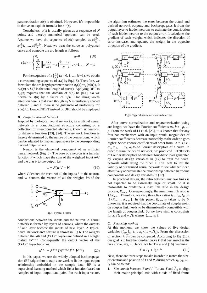
Neuron is the elemental component of an artificial

neural network (Fig. 5). The core of a neuron is a transfer

function F which maps the sum of the weighted input wT𝑰 and the bias b to the output, i.e.

c = F(𝒘𝑇𝑰 + 𝑏) (19)

where 𝑰 denotes the vector of all the inputs Ii to the neuron,

and w denotes the vector of all the weights Wi of the

Fig.5. Typical neuron

connections between the inputs and the neuron. A neural

network is formed by layers of neurons, where the outputs

of one layer become the inputs of next layer. A typical

neural network architecture is shown in Fig 6. The weights

between the kth and (k+1)th layers are defined in a weight

matrix Wk+1,k. Consequently the output vector of the

(k+1)th layer becomes

𝒄𝑘+1 = 𝑭𝑘+1 (𝑾𝑘+1,𝑘𝑰𝑘+1𝒃𝑘+1) (20)

In this paper, we use the widely-adopted backpropaga-

tion (BP) algorithm to train a network to fit the input-output

relationship embedded in the sample data. BP is a

supervised learning method which fits a function based on

samples of input-output data pairs. For each input vector,

the algorithm estimates the error between the actual and

desired network outputs, and backpropagates it from the

output layer to hidden neurons to estimate the contribution

of each hidden neuron to the output error. It calculates the

gradient of each weight, which indicates the direction of

error increase, and updates the weight in the opposite

direction of the gradient.

Fig.6. Typical neural network architecture

After curve normalization and reparametrization using

arc length, we have the Fourier coefficients αk, k = −p, ..., p. From the work of Li et al. [25], it is known that for any

four-bar mechanism with an input crank, magnitudes of

Fourier coefficients decrease noticeably as the order p goes

higher. So we choose coefficients of order from −3 to 3, i.e.,

α-3, α−2, ..., α2, α3 to be Fourier descriptors of a curve. In

order to train the neural network, we produced 101700 sets

of Fourier descriptors of different four-bar curves generated

by varying design variables in (17) to train the neural

network while using the other 101700 sets to test the

validity of our trained neural network to see whether it can

effectively approximate the relationship between harmonic

components and design variables in (17).

In practical design, the ratio between any two links is

not expected to be extremely large or small. So it is

reasonable to predefine a max link ratio in the design

process, 𝐾𝑚𝑎𝑥 . Correspondingly, the minimum link ratio is

1 𝐾𝑚𝑎𝑥⁄ . Therefore, we vary three link ratios 𝑙21, 𝑙31, 𝑙41 in[1 𝐾𝑚𝑎𝑥⁄ , 𝐾𝑚𝑎𝑥] . In this paper, 𝐾𝑚𝑎𝑥 is taken to be 6.

Likewise, it is required that the coordinate of coupler point

on coupler link needs to be dimensionally compatible with

the length of coupler link. So we have similar constraints

for 𝑥𝑐 𝑙3⁄ and 𝑦𝑐 𝑙3⁄ whose 𝜉𝑚𝑎𝑥 is 3.

C. Restoring method

At this moment, we know the values of five design

variables {𝑙21, 𝑙31, 𝑙41, 𝑥𝑐 𝑙3,⁄ 𝑦𝑐 𝑙3⁄ }. From the discussion

of section 4, 𝑃2 can be computed. According to Eq. (16),

our goal is to find the four-bar curve P that best matches the

task curve, say, T. Hence, we let T = P and (16) becomes:

𝑇 = 𝑃1 + 𝑃2𝑒𝑖𝜃1 (21)

Next, there are three steps to take in order to match the size,

orientation and position of T and P, during which 𝑥0, 𝑦0, 𝜃1,

𝑙2 can be found:

1. Size match between T and P. Rotate T and 𝑃2 to align

their major principal axis with 𝑥-axis of fixed frame

respectively and name the transformed curves as R(T)

and R (𝑃2 ). Compute the width or height of the

bounding boxes of R(T) and R(𝑃2) respectively and

denote the ratio as 𝑤1 𝑤2⁄ or ℎ1 ℎ2⁄ , which is the size

ratio between T and 𝑃2. According to Eq. (16), size of

P is determined by 𝑃2 and 𝑃2 is equal to 𝑙1𝑃2 .

Therefore, 𝑙1 = 𝑤1 𝑤2⁄ = ℎ1 ℎ2⁄ .

2. Orientation match between T and P. We obtain the

value of 𝑃2 at step 1 by 𝑙1𝑃2. According to Eq. (16), the

orientation difference between P and 𝑃2 lies on 𝜃1 .

Therefore, 𝜃1 is measured as the angle from the major

principal axis of 𝑃2 to that of T.

3. Position match between T and P. Until now, we know

𝑃2𝑒𝑖𝜃1. Then, we compute the center for T and 𝑃2𝑒𝑖𝜃1

correspondingly and denote them as 𝐶1 and 𝐶2 . The

distance vector from 𝐶2 to 𝐶1 equals to 𝑃1.

Up until now, values of nine design variables in (16) have

been found except for 𝜙0 . As said earlier, 𝜙0 only

determines the starting point of curve and is irrelevant to

position, orientation, size and shape of curve. In practical

use, the starting point can be chosen according to the needs

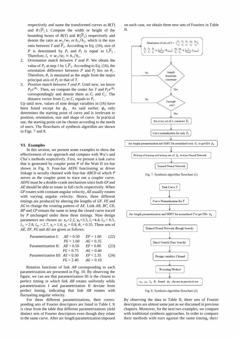
of users. The flowcharts of synthesis algorithm are shown

in Figs. 7 and 8.

VI. Examples

In this section, we present some examples to show the

effectiveness of our approach and compare with Wu’s and

Chu’s methods respectively. First, we present a task curve

that is generated by coupler point P of the Watt II six-bar

shown in Fig. 9. Four-bar AEFG functioning as driver

linkage is serially chained with four-bar ABCD of which P serves as the coupler point to trace out a coupler curve.

AEFG must be a double-crank mechanism since both GF and

AE should be able to rotate in full circle respectively. When

GF rotates with constant angular velocity, AE usually rotates

with varying angular velocity. Hence, three different

timings are produced by altering the lengths of GF, FE and

AG to change the rotating pattern of AE. Link AB, BC, CD,

BP and CP remain the same to keep the closed curve traced

by P unchanged under these three timings. Nine design

parameters are chosen as: 𝑥0=2.2, 𝑦0=3.5, 𝑙1=4.4, 𝑙21= 0.5, 𝑙31 = 2.8, 𝑙41 = 2.7, 𝑥𝑐= 1.0, 𝑦𝑐 = 0.8, 𝜃1 = 0.55. Three sets of

AE, EF, FG and AG are given as follows:

Parametrization I: AE = 0.50 EF = 1.60 (22)

FG = 1.60 AG = 0.35

Parametrization II: AE = 0.50 EF = 0.80 (23)

FG = 0.75 AG = 0.40

Parametrization III: AE = 0.50 EF = 2.35 (24)

FG = 2.40 AG = 0.10

Rotation functions of link AB corresponding to each

parametrization are presented in Fig. 10. By observing the

figure, we can see that parametrization III is the closest to

perfect timing in which link AB rotates uniformly while

parametrization I and parametrization II deviate from

perfect timing, indicating that link AB rotates with

fluctuating angular velocity.

For these different parametrizations, their corres-

ponding sets of Fourier descriptors are listed in Table I. It

is clear from the table that different parametrizations yield

distinct sets of Fourier descriptors even though they relate

to the same curve. After arc length parametrization imposed

on each case, we obtain three new sets of Fouriers in Table

II.

Fig. 7. Synthesis algorithm flowchart (1)

Fig. 8. Synthesis algorithm flowchart (2)

By observing the data in Table II, three sets of Fourier

descriptors are almost same just as we discussed in previous

chapters. Moreover, for the next two examples, we compare

with traditional synthesis approaches. In order to compare

their methods with ours against the same timing, their

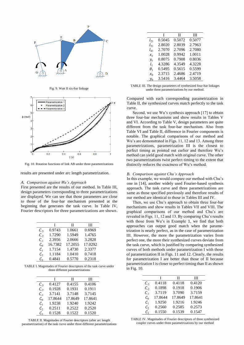
Fig. 9. Watt II six-bar linkage

Fig. 10. Rotation functions of link AB under three parametrizations

results are presented under arc length parametrization.

A. Comparison against Wu’s Approach

First presented are the results of our method. In Table III,

design parameters corresponding to three parametrizations

are displayed. We can see that those parameters are close

to those of the four-bar mechanism presented at the

beginning that generates the task curve. In Table IV,

Fourier descriptors for three parametrizations are shown.

I II III

𝐶-3 0.9743 1.0661 0.6969

𝐶-2 1.7290 1.5949 1.4765

𝐶-1 2.3956 2.0666 3.2828

𝐶0 16.7382 17.2055 17.0292

𝐶1 1.7154 1.4730 2.3377

𝐶2 1.1184 1.0410 0.7418

𝐶3 0.4841 0.5770 0.2318

TABLE I. Magnitudes of Fourier descriptors of the task curve under

three different parametrizations

I II III

𝐶-3 0.4127 0.4155 0.4106

𝐶-2 0.1928 0.1931 0.1911

𝐶-1 3.7141 3.7148 3.7145

𝐶0 17.8644 17.8649 17.8641

𝐶1 1.9238 1.9240 1.9242

𝐶2 0.2511 0.2522 0.2520

𝐶3 0.1528 0.1522 0.1520

TABLE II. Magnitudes of Fourier descriptors (after arc length

parametrization) of the task curve under three different parametrizations

I II III

𝑙21 0.5045 0.5072 0.5077

𝑙31 2.8020 2.8039 2.7963

𝑙41 2.7070 2.7096 2.7080

𝑥𝑐 1.0028 0.9942 1.0011

𝑦𝑐 0.8075 0.7908 0.8036

𝑙1 4.3286 4.3549 4.3228

𝜃1 0.5495 0.5615 0.5599

𝑥0 2.3715 2.4686 2.4719

𝑦0 3.5416 3.4464 3.5058

TABLE III. The design parameters of synthesized four-bar linkages

under three parametrizations by our method.

Compared with each corresponding parametrization in

Table II, the synthesized curves match perfectly to the task

curve.

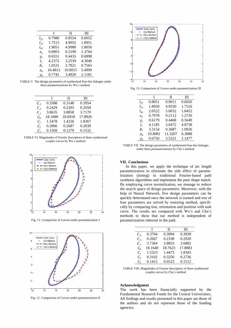
Second, we use Wu’s synthesis approach [17] to obtain

three four-bar mechanisms and show results in Tables V

and VI. According to Table V, design parameters are quite

different from the task four-bar mechanism. Also from

Table VI and Table II, difference in Fourier components is

notable. The graphical comparisons of our method and

Wu’s are demonstrated in Figs. 11, 12 and 13. Among three

parametrizations, parametrization III is the closest to

perfect timing as pointed out earlier and therefore Wu’s

method can yield good match with original curve. The other

two parametrizations twist perfect timing to the extent that

distinctly reduces the exactness of Wu’s method.

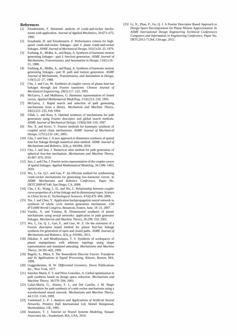
B. Comparison against Chu’s Approach

In this example, we would compare our method with Chu’s

one in [14], another widely used Fourier-based synthesis

approach. The task curve and three parametrizations are

same as those specified previously and therefore results of

our method are identical to those in Tables III and IV.

Then, we use Chu’s approach to obtain three four-bar

mechanisms and show results in Tables VII and VIII. The

graphical comparisons of our method and Chu’s are

revealed in Figs. 11, 12 and 13. By comparing Chu’s results

with those from Wu’s in Example 1, we find that both

approaches can output good match when the parame-

trization is nearly perfect, as in the case of parametrization

III. However, the more the parametrization varies from

perfect one, the more their synthesized curves deviate from

the task curve, which is justified by comparing synthesized

curves of both methods under parametrization I with those

of parametrization II in Figs. 11 and 12. Clearly, the results

for parametrization I are better than those of II because

parametrization I is closer to perfect timing than II as shown

in Fig. 10.

I II III

𝐶-3 0.4118 0.4118 0.4120

𝐶-2 0.1898 0.1918 0.1906

𝐶-1 3.7119 3.7090 3.7159

𝐶0 17.8644 17.8649 17.8641

𝐶1 1.9250 1.9216 1.9246

𝐶2 0.2560 0.2585 0.2573

𝐶3 0.1550 0.1539 0.1547

TABLE IV. Magnitudes of Fourier descriptors of three synthesized

coupler curves under three parametrizations by our method

I II III

𝑙21 0.7980 0.8554 0.6052

𝑙31 1.7515 4.9052 1.8951

𝑙41 1.9051 4.9980 1.8050

𝑥𝑐 0.8903 0.2190 1.3764

𝑦𝑐 0.6551 0.4433 0.6998

𝑙1 4.2372 3.2539 4.3040

𝜃1 1.0531 2.7821 0.7563

𝑥0 10.4813 10.8015 5.4999

𝑦0 0.7741 3.4920 2.1181

TABLE V. The design parameters of synthesized four-bar linkages under

three parametrizations by Wu’s method.

I II III

𝐶-3 0.3588 0.3148 0.3954

𝐶-2 0.2429 0.2303 0.2058

𝐶-1 3.8635 3.8858 3.7170

𝐶0 18.1680 18.6918 17.8926

𝐶1 1.5478 1.4226 1.8367

𝐶2 0.2866 0.2687 0.2839

𝐶3 0.1569 0.1279 0.1532

TABLE VI. Magnitudes of Fourier descriptors of three synthesized

coupler curves by Wu’s method

Fig. 11. Comparison of Curves under parametrization I

Fig. 12. Comparison of Curves under parametrization II

Fig. 13. Comparison of Curves under parametrization III

I II III

𝑙21 0.8051 0.9011 0.6050

𝑙31 1.8950 4.9550 1.7516

𝑙41 2.0522 5.0032 1.8452

𝑥𝑐 0.7978 0.2112 1.2720

𝑦𝑐 0.6179 0.4468 0.5649

𝑙1 4.1185 3.0472 4.8738

𝜃1 3.3154 0.3687 1.0926

𝑥0 10.8081 11.3207 6.3888

𝑦0 0.6750 3.5521 1.1477

TABLE VII. The design parameters of synthesized four-bar linkages

under three parametrizations by Chu’s method.

VII. Conclusions

In this paper, we apply the technique of arc length

parametrization to eliminate the side effect of parame-

trization (timing) in traditional Fourier-based path

synthesis algorithms and implement the pure shape match.

By employing curve normalization, we manage to reduce

the search space of design parameters. Moreover, with the

help of Neural Network, five design parameters can be

quickly determined once the network is trained and rest of

four parameters are solved by restoring method, specifi-

cally by comparing size, orientation and position with task

curve. The results are compared with Wu’s and Chu’s

methods to show that our method is independent of

parametrization inherent in the path.

I II III

𝐶-3 0.3704 0.3994 0.3939

𝐶-2 0.2667 0.2338 0.2020

𝐶-1 3.7364 3.8833 3.6882

𝐶0 18.1640 18.7623 17.8883

𝐶1 1.5323 1.4473 1.8343

𝐶2 0.3102 0.3250 0.2736

𝐶3 0.1415 0.0523 0.1512

TABLE VIII. Magnitudes of Fourier descriptors of three synthesized

coupler curves by Chu’s method

Acknowledgment

The work has been financially supported by the

Fundamental Research Funds for the Central Universities.

All findings and results presented in this paper are those of

the authors and do not represent those of the funding

agencies.

References [1] Freudenstein, F. Harmonic analysis of crank-and-rocker mecha-

nisms with application. Journal of Applied Mechanics, 26:673–675,

1960. [2] Funabashi, H. and Freudenstein, F. Performance criteria for high-

speed crank-and-rocker linkages—part I: plane crank-and-rocker

linkages. ASME Journal of Mechanical Design, 101(1):20–25, 1979. [3] Fanhang, K., Midha, A., and Bajaj, A. Synthesis of harmonic motion

generating linkages—part I: function generation. ASME Journal of

Mechanisms, Transmissions, and Automation in Design, 110(1):16–

21, 1988. [4] Fanhang, K., Midha, A., and Bajaj, A. Synthesis of harmonic motion

generating linkages—part II: path and motion generation. ASME

Journal of Mechanisms, Transmissions, and Automation in Design,

110(1):22–27, 1988. [5] Chu, J. and Cao, W. Synthesis of coupler curves of planar four-bar

linkages through fast Fourier transform. Chinese Journal of

Mechanical Engineering, 29(5):117–122, 1993. [6] McGarva, J. and Mullineux, G. Harmonic representation of closed

curves. Applied Mathematical Modelling, 17(4):213–218, 1993. [7] McGarva, J. Rapid search and selection of path generating

mechanisms from a library. Mechanism and Machine Theory,

29(2):223–235, Feb 1994. [8] Ullah, L. and Kota, S. Optimal synthesis of mechanisms for path

generation using Fourier descriptor and global search methods.

ASME Journal of Mechanical Design, 119(4):504–510, 1997. [9] Nie, X. and Krovi, V. Fourier methods for kinematic synthesis of

coupled serial chain mechanisms. ASME Journal of Mechanical

Design, 127(1):232–241, 2005. [10] Chu, J. and Sun, J. A new approach to dimension synthesis of spatial

four-bar linkage through numerical atlas method. ASME Journal of

Mechanisms and Robotics, 2(4), p. 041004, 2010. [11] Chu, J. and Sun, J. Numerical atlas method for path generation of

spherical four-bar mechanism. Mechanisms and Machine Theory,

45:867–879, 2010. [12] Sun, J. and Chu, J. Fourier series representation of the coupler curves

of spatial linkages. Applied Mathematical Modeling, 34:1396–1403,

2010. [13] Wu, J., Ge, Q.J., and Gao, F. An efficient method for synthesizing

crank-rocker mechanisms for generating low-harmonic curves. In

ASME Mechanisms and Robotics Conference, Paper No.

DETC2009-87140, San Diego, CA, 2009. [14] Chu, J. K., Wang, L. D., and Wu, C. Relationship between coupler

curve properties of a 4-bar linkage and its dimensional types. Science

in China Series E: Technological Sciences, 47(4):479–484, 2004. [15] Xie, J. and Chen, Y. Application backpropagation neural network to

synthesis of whole cycle motion generation mechanism. 12th

IFToMM World Congress, Besancon, France, June, 18–21, 2007. [16] Vasiliu, A. and Yannou, B. Dimensional synthesis of planar

mechanisms using neural networks: application to path generator

linkages. Mechanism and Machine Theory, 36:299–310, 2001. [17] Wu, J., Ge, Q. J., Gao, F., and Guo, W. Z. On the extension of a

Fourier descriptor based method for planar four-bar linkage

synthesis for generation of open and closed paths. ASME Journal of

Mechanisms and Robotics, 3(3), p. 031002, 2011. [18] Dikabar, S. and Mruthyunjaya, T. S. Synthesis of workspaces of

planar manipulators with arbitrary topology using shape

representation and simulated annealing. Mechanisms and Machine

Theory, 34:391-420, 1999. [19] Bagchi, S., Mitra, S. The Nonuniform Discrete Fourier Transform

and its Applications in Signal Processing, Kluwer, Boston, MA, 1999.

[20] Guggenheimer, H. W. Differential Geometry. Dover Publications

Inc., New York, 1977. [21] Sánchez Marín, F. T. and Pérez González, A. Global optimization in

path synthesis based on design space reduction. Mechanisms and

Machine Theory, 38:579–594, 2003. [22] Galán-Marín, G., Alonso, F. J., and Del Castillo, J. M. Shape

optimization for path synthesis of crank-rocker mechanisms using a

wavelet-based neural network. Mechanisms and Machine Theory,

44:1132–1143, 2009. [23] Veelenturf, L. P. J. Analysis and Applications of Artificial Neural

Networks, Prentice Hall International Ltd, Hemel Hempstead,

Hertfordshire, UK, 1995. [24] Anastasio, T. J. Tutorial on Neural Systems Modeling, Sinauer

Associates Inc., Sunderland, MA, USA, 2010.

[25] Li, X., Zhao, P., Ge, Q. J. A Fourier Descriptor Based Approach to

Design Space Decomposition for Planar Motion Approximation. In

ASME International Design Engineering Technical Conferences

Computers and Information in Engineering Conference, Paper No.

DETC2012-71264, Chicago, 2012.