1
Optimal supply chain design and management over a multi-period horizon under demand uncertainty. Part I: MINLP and MILP models
Maria Analia Rodriguez1, Aldo R. Vecchietti1, Iiro Harjunkoski2 and Ignacio E. Grossmann2
1INGAR (CONICET-UTN), Avellaneda 3657, Santa Fe 3000, Argentina
2ABB AG, Corporate Research Germany, Wallstadter Straße 59, 68526 Ladenburg, Germany 3Center for Advanced Process Decision-making, Department of Chemical Engineering, Carnegie Mellon
University, Pittsburgh, PA 15217, USA
Abstract An optimization model is proposed to redesign the supply chain of spare part delivery under demand
uncertainty in a specified planning horizon. Long term decisions involve new installations, expansions and
elimination of warehouses handling multiple products. It is considered which warehouses should be used as
repair work-shops to store, repair and deliver used units to customers. Tactical planning includes deciding
inventory, and the connection links between the supply chain nodes. At the tactical level it is determined how
demand of failing units is satisfied, and whether to use new or used parts. The uncertain demand is addressed by
defining the optimal amount of safety stock that guarantees certain service level at a customer plant. Due to the
nonlinear nature of the original formulation, a piece-wise linearization approach is applied to obtain a tight
lower bound of the optimal solution. The formulation is applied to the supply chain of electric motors.
Keywords: supply chain, demand uncertainty, inventory management, mixed integer non-linear
programming
1. Introduction
The integration of supply chain redesign and tactical decisions such as defining inventory levels and
how supply chain nodes are connected is a challenging problem that can greatly impact the financial
performance of a company. Rising transportation costs are key factors in decisions about where to place
factories and distribution centers, and how much inventory to store. In addition, optimal inventory
management has become a major goal in order to simultaneously reduce costs and improve customer
service in today’s increasingly competitive business environment (Daskin, Coullard and Shen, 2002). For
that reason, over the last few years, there has been an increasing interest in developing enterprise-wide
optimization (EWO) models to solve problems that are broad in scope and integrate several decision
levels (Grossmann, 2005). EWO involves optimizing the operations of supply, manufacturing and
distribution activities of a company to reduce costs, inventories and environmental impact, and to
maximize profits and responsiveness.
Given a supply chain where some plants and distribution centers are already installed, the
redesign problem consist of deciding on new investments as well as eliminating installed assets that
are not profitable. Considering these types of decisions as an isolated problem, without taking into
account certain tactical and operational decisions, could have a negative impact on the performance of
2
the supply chain. Investment decisions in a supply chain directly affect transportation and inventory
costs. Therefore, an integrated approach is required to obtain a more flexible and efficient supply
chain.
In the particular case of the electric motors industry, the relevance of this problem is given by
some key issues. On the one hand, electric motors are expensive products, so keeping them in
inventory means tying a significant amount of capital. On the other hand, a motor malfunction may
block the entire production of a customer’s plant, and therefore obtaining a spare motor as soon as
possible is critical. The same applies to e.g. wind generators, where energy is the only product.
Another special characteristic of this type of industry is given by the type of product. Most
contributions in the literature assume that products are only moved forward in the supply chain, and
only the demand of new products is considered. In this case, the situation is more complex. As usual,
demand can be originated by new customers or new investments at customer sites. However, in
addition, motors or other units that are already in use can fail. In this case, clients require replacing the
failed component. An important decision in this context is whether to replace failed parts with new
units or with repaired products. The latter give rise to reverse flows since failed units must be shipped
from the customers to the service centers for repair. An efficient inventory management of new and
used units in the supply chain warehouses is another challenge of this problem.
Customer plants typically have tens or more different types of motors or other units in their
production processes, and identical units can be used for a variety of purposes. According to the type
of unit and its application, the criticality of a given unit can be very different so the time a customer
can wait for a replacement is case dependent. If the time requirement is very tight, it might be
necessary to have some emergency stock at the customer sites.
Taking into account that e.g. a motor demand is uncertain and that it depends on the failure rate, a
responsive supply chain can only be guaranteed when an effective inventory management, as well as
an appropriate distribution and storage structure are planned together. Furthermore, demand
uncertainty might also have a relevant influence on the warehouse capacities. In that sense, if the plan
for storage capacity does not consider demand uncertainty, it might be infeasible to provide the spare
parts as required.
You and Grossmann (2010) propose an optimization model to design a multi-echelon supply
chain and the associated inventory systems under demand uncertainty in the chemical industry. The
original model is a Mixed Integer Non-Linear Programming problem (MINLP) with a non-convex
objective function for which they develop a spatial decomposition algorithm to obtain near global
optimal solutions with reasonable computational expense. The supply chain involves one product, and
design decisions consider the installation of new distribution centers, but no expansions or elimination
of installed warehouses are considered since the model assumes only one planning period. Our
approach extends this previous work introducing new considerations regarding the particular
3
industrial context for electric motors and other similar parts, and complexities from the modeling
point of view and novel concepts that were not considered before.
We develop an optimization model to redesign the supply chain of spare parts or units under
demand uncertainty from strategic and tactical perspectives in a planning horizon consisting of
multiple periods. The main objective is to redesign an optimal supply chain for the spare parts
minimizing costs and deciding where to place warehouses, which installed warehouses should be
eliminated, what are the stock capacities and safety stocks required, as well as how to connect the
different echelons of the supply chain in order to satisfy uncertain demand of spare parts.
The uncertain demand is addressed by defining the optimal amount of safety stock that guarantees
certain service level at a customer plant. In addition, the risk-pooling effect described by Eppen
(1979) is taken into account when defining inventory levels in distribution centers and customer
zones. One additional consideration is given by the inclusion of lost sales costs in the objective
function, which was extended from the work by Parker (1964). Due to the nonlinear and large size
nature of the original formulation, apiece-wise linearization algorithms applied to obtain the optimal
solution.
This article is organized as follows. In section 2, a brief literature review is presented showing
different approaches to represent de demand uncertainty as well as the analysis of inventory systems
under deterministic and uncertain contexts. The major objective of section 3 is to characterize and
describe the problem addressed in this article, giving some details regarding the challenges, industry
issues and main decisions considered. Section 4 presents the approach applied in this work to handle
demand uncertainty and some new considerations related to lost sales. The model formulation is
presented in section 5 while section 6 describes the solution approach. Sections 7 and 8 show results
and conclusions, respectively.
2. Literature Review
2.1. Previous works
Some previous work from the literature address similar problems as the one in this paper. Daskin
et al. (2002) introduce an inventory-location model in which supply chain design decisions integrate
inventory considerations in order to minimize investment and logistic costs under demand uncertainty.
It is assumed that the connection between plants and distribution centers is given. No limitation in
storage and production capacity is considered and all delivery times from supplier to distribution
centers are the same. Given these assumptions and since storage decisions at customer sites are
disregarded, the inventory structure is considered as a single echelon system. A similar approach can
be found in Shen et al. (2003). Extending this approach, You and Grossmann (2008) formulate an
MINLP model and develop effective algorithms for large-scale instances.
Santoso et al. (2005) propose a stochastic programming model and solution algorithm for solving
supply chain network design problems of realistic size. Their solution methodology integrates the
4
sample average approximation (SAA) scheme, with an accelerated Benders decomposition algorithm
to compute high quality solutions to large-scale stochastic supply chain design problems with a large
number of scenarios. The model decides which facilities to install, and how different nodes should be
linked in order to minimize investment, operating and transportation costs. However, inventory
management and the associated costs are neglected. Since design decisions are assumed over one
period, no expansion or elimination of processing facilities are considered. Bossert and Willems
(2007) extend the guaranteed service modeling framework in order to optimize the inventory policy in
a supply chain. Although they address numerous real world complexities regarding inventory
management, no design decisions are considered since the supply chain configuration is defined a
priori.
2.2. Approachesto model demand uncertainty
In order to cope with demand uncertainty, there are two main approaches to consider. The first
one uses a stochastic programming model where uncertainty is considered directly using a scenario
based approach (Sahinidis, 2004). Each scenario is associated with certain probability of occurrence
and represents one possible realization for the uncertain parameter. In general, there are two or more
stages in the decision process. In the first stage, ‘here and now’ decisions have to be made before the
uncertain parameter realization is known. In the second stage, ‘wait and see’ decisions are considered
which are associated with a recourse action because they can be made after the random parameter is
known. The main disadvantage of this method is that the model size tends to increase rapidly with the
number of scenarios considered. In addition, it is not always feasible to explicitly enumerate all
possible discrete values of the uncertain parameter.
The second approach is to use chance constraint approach in which each uncertain parameter is
treated as a random variable with a given probability distribution (Charnes and Cooper, 1963),
which is applied in several cases to model demand uncertainty (Gupta and Maranas, 2003, You and
Grossmann, 2008, Rodriguez and Vecchietti, 2011). Applying this approach the demand
uncertainty is considered by specifying a demand level above the mean that must be satisfied. In this
way, one strategy proposed by You and Grossmann (2008) is to define the safety stock as a decision
variable in the model and a guaranteed service level to reduce the shortage in the inventories. Even
though this approach does not involve scenarios, the model gives rise to non-linearities in the
formulation.
Given the type of problem considered, if a two-stage stochastic approach were used, the design
decision would be selected in a first stage, before demand is realized, and inventory levels would be
determined after demand is known. However, since the product under consideration can be critical to
a customer, the lead time that the customer has to wait until the unit is ready to be used is an
important variable. In fact, the lead time accepted by the customers might be rather short when a spare
part fails, so a recourse action would not be a feasible option in all cases. The second approach is
5
chosen because it defines a safety stock level at customer sites and warehouses in order to guarantee
the customer requirements.
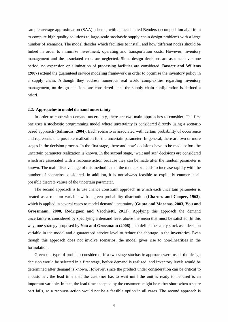
2.3. Inventory evolution vs. demand in the deterministic and the uncertain cases
From the inventory management point of view, one traditional strategy to handle inventory is to
consider a base stock policy which is also called order-up-to-level policy (Zipkin, 2000). Using this
method, the inventory is reviewed in every time period, and the amount ordered is determined by the
difference between the base stock level and the inventory level at the time of review. If the demand is
deterministic, a constant demand rate is assumed so that in every period the same amount is ordered,
which is exactly the total demand expected during the lead time period. This situation does not hold
when there is uncertainty. Uncertain demand means that the exact amount that will be ordered by
customers during the inventory period is not known in advance even though some probabilistic
information regarding the demand can be assumed. If the inventory level is not properly planned, and
the demand is greater than expected, lost sales or back-orders will take place. On the contrary, if the
demand is lower than forecasted, there will be an excess in the inventory level. Figures 1-a and 1-b
show different stock evolutions in time horizon, considering deterministic and uncertain demand,
respectively. In our approach, we determine a minimum level of products to keep in stock (safety
stock) in order to guarantee that certain demand increase will be satisfied. In this case, stock evolution
is shown in Figure 1-c.
Figure 1-a. Stock evolution with Figure 1-b. Stock evolution with uncertain demand deterministic demand
Figure 1-c. Stock evolution with uncertain demand and safety stock
-2
0
2
4
6
8
10
12
14
16
0 5 10 15 20
Inventory level
days
Units
in in
vent
ory
-4
-2
0
2
4
6
8
10
12
14
16
0 5 10 15 20
Inventory level
Units
in in
vent
ory
days
-4-202468
10121416
0 5 10 15 20
Inventory level with safety stock
Safety stock
days
Units
in in
vent
ory
Shortage
6
3. Supply chain redesign in the for spare parts
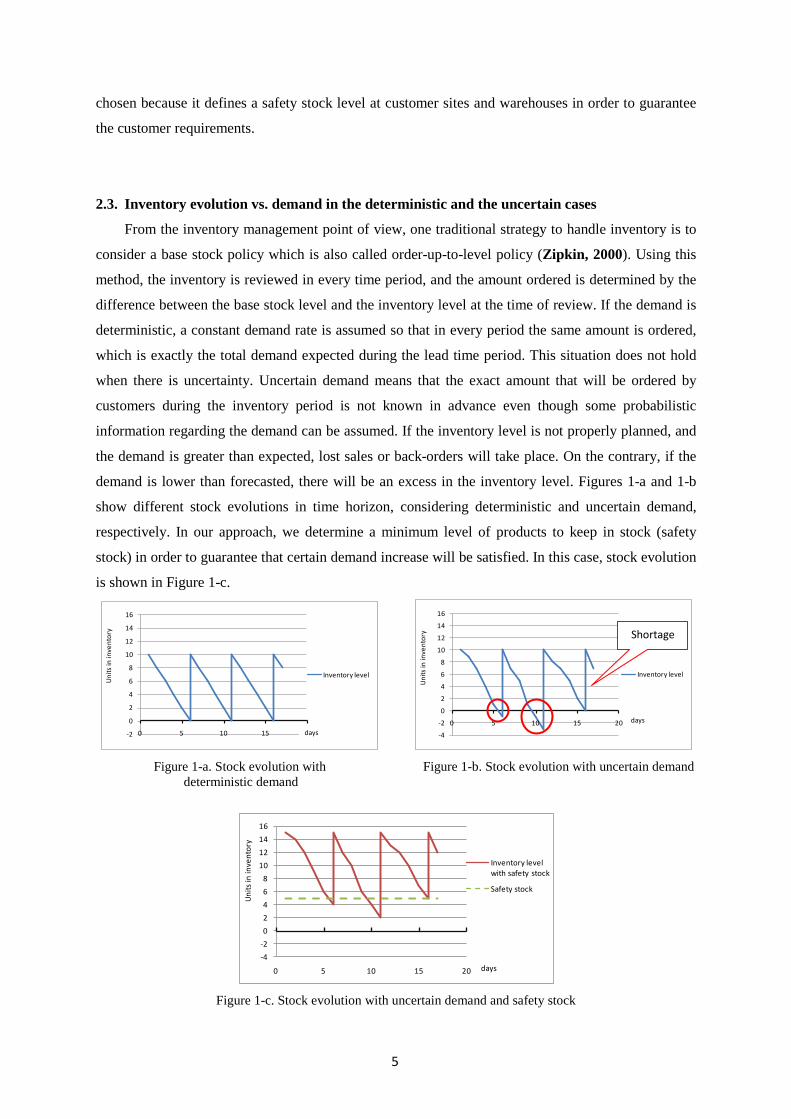
3.1. Traditional supply chain redesign decisions
A three echelon supply chain with a given set of factories and warehouses that produce and deliver
multiple spare units to end customers is considered.
Long term decisions involve new installations, expansions, and elimination of factories and
warehouses. It is also decided which warehouses should be used as repair work-shops in order to
store, repair and deliver the used (repaired) units to customers. In addition, the links between
factories, warehouses and end customers must be selected. We assume that several factories can
provide one warehouse with the same spare part, while each end customer is assumed to be served by
only one warehouse. Figure 2 represents the main design decisions in the supply chain structure, while
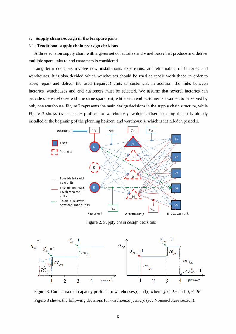
Figure 3 shows two capacity profiles for warehouse j1 which is fixed meaning that it is already
installed at the beginning of the planning horizon, and warehouse j2 which is installed in period 1.
Figure 2. Supply chain design decisions
Figure 3. Comparison of capacity profiles for warehouses j1 and j2 where 1j JF∈ and 2j JF∉
Figure 3 shows the following decisions for warehouses j1 and j2 (see Nomenclature section):
k5
i1
i2
i3
j1
j2
j3
j4
k1
k2
k3
k4
Factories i Warehouses j End Customer k
wit xijpt yjt zjktDecisions
Fixed
Potential
Possible links with new unitsPossible links with used (repaired) units
uikst vjkst
Possible links with new tailor made units
7
• Warehouse j1 is already installed in the supply chain and the initial capacity is given by
1jIC . It is expanded in the first period which is indicated by binary variable
1 11e
j ty = .
Capacity expansion is given by 1 1j tce . The same decision is made in period 3.
• Warehouse j2 is installed in period 1 which is indicated by 2 1
1j ty = . This capacity
expansion is given by 2 1j tce . This warehouse is expanded again in period 3. Therefore,
total capacity in period 3 is given by 2 3 2 1 2 3j t j t j tq ce ce= + . In period 4 this warehouse is
eliminated from the supply chain, this is decided by 2 4
1uj ty = and the capacity uninstalled is
given by 2 4j tuc .
3.2. Types of products
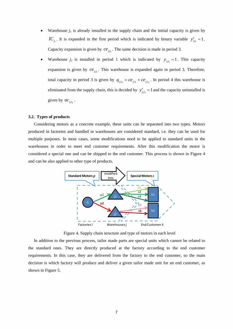
Considering motors as a concrete example, these units can be separated into two types. Motors
produced in factories and handled in warehouses are considered standard, i.e. they can be used for
multiple purposes. In most cases, some modifications need to be applied to standard units in the
warehouses in order to meet end customer requirements. After this modification the motor is
considered a special one and can be shipped to the end customer. This process is shown in Figure 4
and can be also applied to other type of products.
Figure 4. Supply chain structure and type of motors in each level
In addition to the previous process, tailor made parts are special units which cannot be related to
the standard ones. They are directly produced at the factory according to the end customer
requirements. In this case, they are delivered from the factory to the end customer, so the main
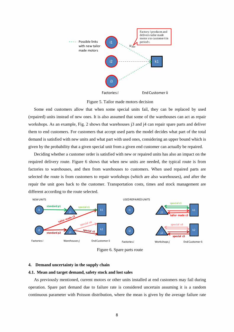
decision is which factory will produce and deliver a given tailor made unit for an end customer, as
shown in Figure 5.
i1
j1
j2
k1
Standard Motors p modified into
p1
p2
k2
s1 s2 s3
s4
s5
Special Motors s
Factories i Warehouses j End Customer k
8
Figure 5. Tailor made motors decision
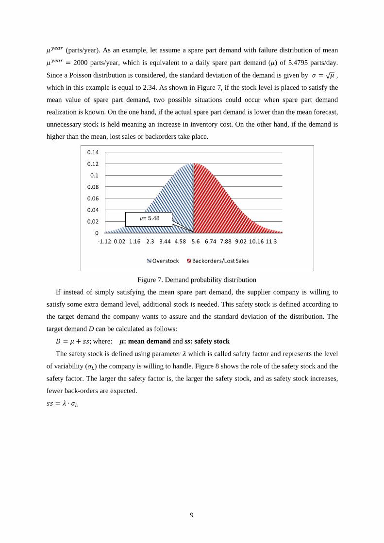
Some end customers allow that when some special units fail, they can be replaced by used
(repaired) units instead of new ones. It is also assumed that some of the warehouses can act as repair
workshops. As an example, Fig. 2 shows that warehouses j3 and j4 can repair spare parts and deliver
them to end customers. For customers that accept used parts the model decides what part of the total
demand is satisfied with new units and what part with used ones, considering an upper bound which is
given by the probability that a given special unit from a given end customer can actually be repaired.
Deciding whether a customer order is satisfied with new or repaired units has also an impact on the
required delivery route. Figure 6 shows that when new units are needed, the typical route is from
factories to warehouses, and then from warehouses to customers. When used repaired parts are
selected the route is from customers to repair workshops (which are also warehouses), and after the
repair the unit goes back to the customer. Transportation costs, times and stock management are
different according to the route selected.
Figure 6. Spare parts route
4. Demand uncertainty in the supply chain
4.1. Mean and target demand, safety stock and lost sales
As previously mentioned, current motors or other units installed at end customers may fail during
operation. Spare part demand due to failure rate is considered uncertain assuming it is a random
continuous parameter with Poisson distribution, where the mean is given by the average failure rate
i1
i2
i3
k1
uikst
Factories i End Customer k
Factory i produces and delivers tailor made motor s to customer k in period t.Possible links
with new tailor made motors
i1j1
j2
k1standard p1
k2
special s1
Factories i Warehouses j End Customer k
i2standard p2
NEW UNITS
i1j1
j2
k1
tailor made s3
k2
special s1
special s4
special s5
Factories i Workshops j End Customer k
i2
USED REPAIRED UNITS
9
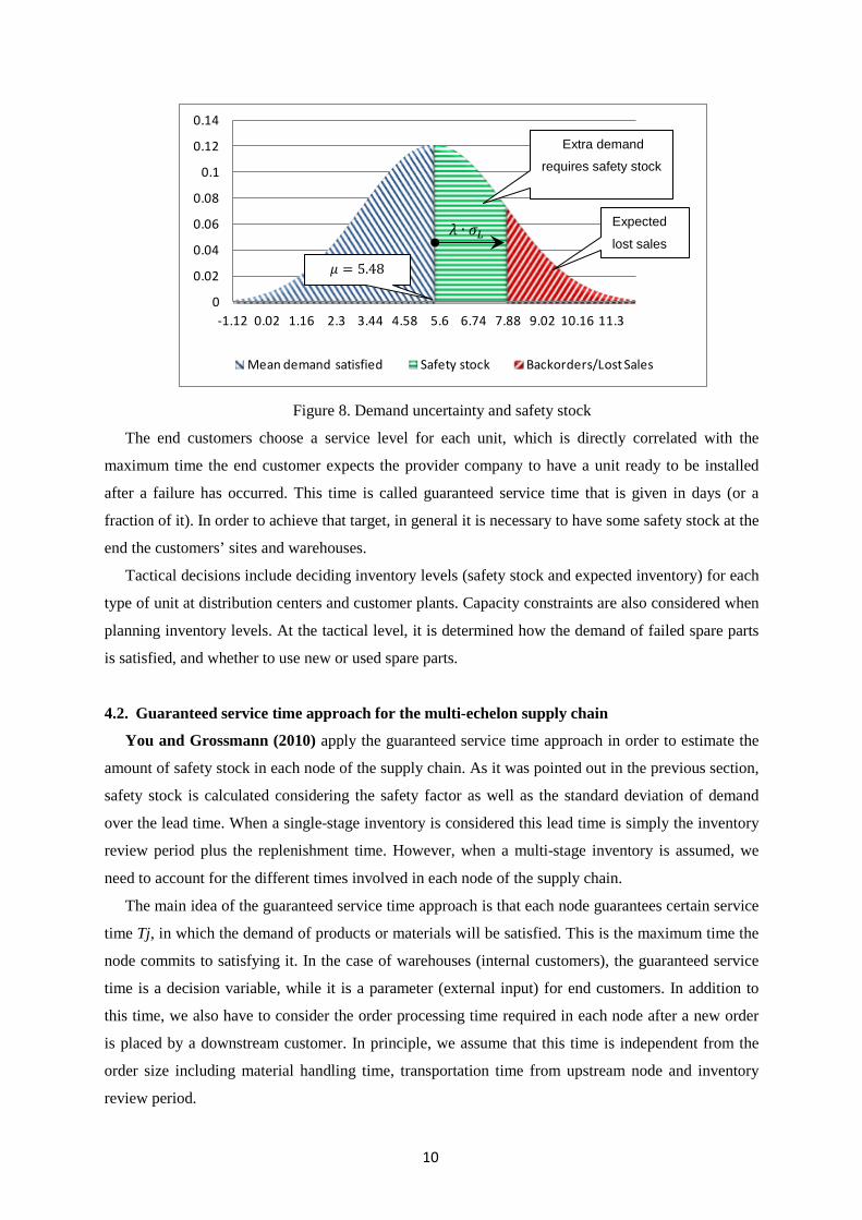
𝜇𝑦𝑒𝑎𝑟 (parts/year). As an example, let assume a spare part demand with failure distribution of mean
𝜇𝑦𝑒𝑎𝑟 = 2000 parts/year, which is equivalent to a daily spare part demand (𝜇) of 5.4795 parts/day.
Since a Poisson distribution is considered, the standard deviation of the demand is given by 𝜎 = √𝜇 ,
which in this example is equal to 2.34. As shown in Figure 7, if the stock level is placed to satisfy the
mean value of spare part demand, two possible situations could occur when spare part demand
realization is known. On the one hand, if the actual spare part demand is lower than the mean forecast,
unnecessary stock is held meaning an increase in inventory cost. On the other hand, if the demand is
higher than the mean, lost sales or backorders take place.
Figure 7. Demand probability distribution
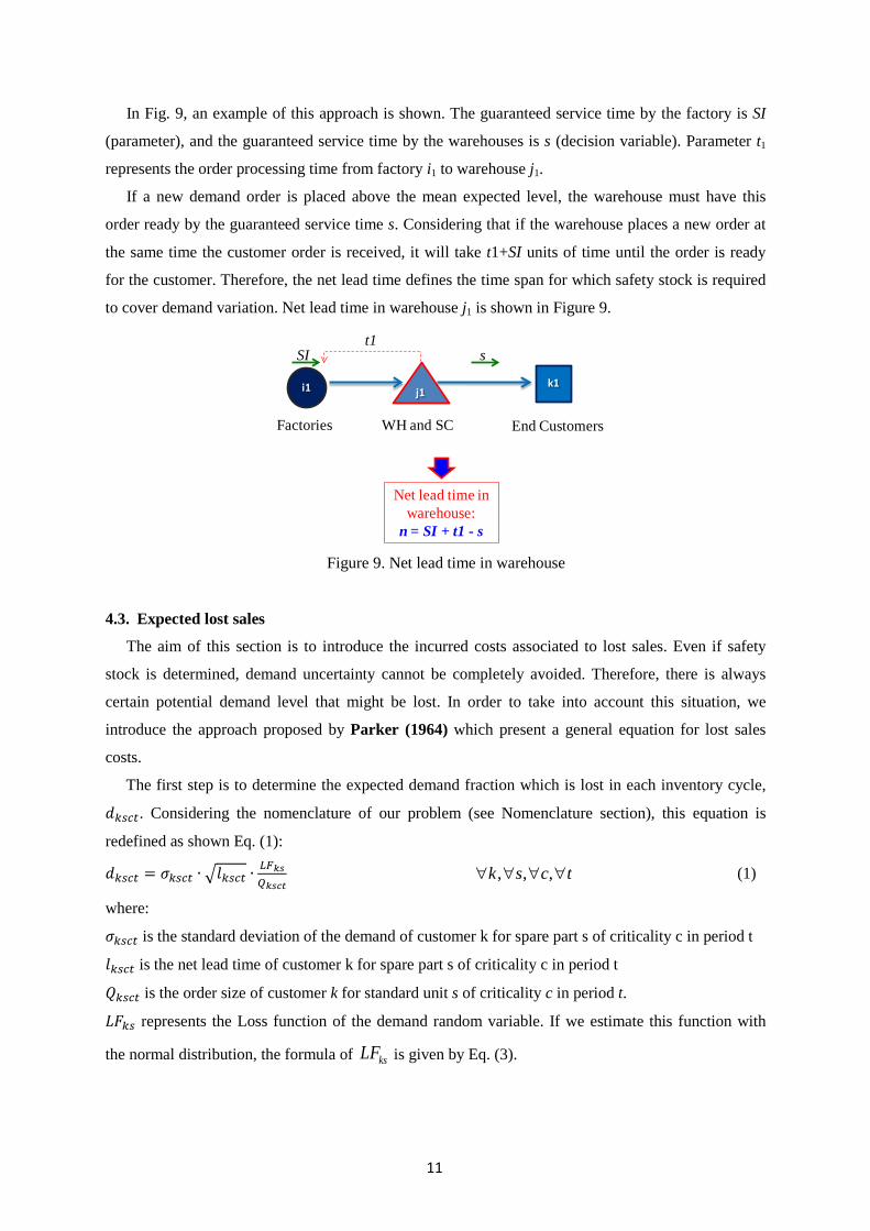
If instead of simply satisfying the mean spare part demand, the supplier company is willing to
satisfy some extra demand level, additional stock is needed. This safety stock is defined according to
the target demand the company wants to assure and the standard deviation of the distribution. The
target demand D can be calculated as follows:
𝐷 = 𝜇 + 𝑠𝑠; where: 𝝁: mean demand and ss: safety stock
The safety stock is defined using parameter 𝜆 which is called safety factor and represents the level
of variability (𝜎𝐿) the company is willing to handle. Figure 8 shows the role of the safety stock and the
safety factor. The larger the safety factor is, the larger the safety stock, and as safety stock increases,
fewer back-orders are expected.
𝑠𝑠 = 𝜆 ∙ 𝜎𝐿
0
0.02
0.04
0.06
0.08
0.1
0.12
0.14
-1.12 0.02 1.16 2.3 3.44 4.58 5.6 6.74 7.88 9.02 10.16 11.3
Overstock Backorders/Lost Sales
𝜇= 5.48
10
Figure 8. Demand uncertainty and safety stock
The end customers choose a service level for each unit, which is directly correlated with the
maximum time the end customer expects the provider company to have a unit ready to be installed
after a failure has occurred. This time is called guaranteed service time that is given in days (or a
fraction of it). In order to achieve that target, in general it is necessary to have some safety stock at the
end the customers’ sites and warehouses.
Tactical decisions include deciding inventory levels (safety stock and expected inventory) for each
type of unit at distribution centers and customer plants. Capacity constraints are also considered when
planning inventory levels. At the tactical level, it is determined how the demand of failed spare parts
is satisfied, and whether to use new or used spare parts.
4.2. Guaranteed service time approach for the multi-echelon supply chain
You and Grossmann (2010) apply the guaranteed service time approach in order to estimate the
amount of safety stock in each node of the supply chain. As it was pointed out in the previous section,
safety stock is calculated considering the safety factor as well as the standard deviation of demand
over the lead time. When a single-stage inventory is considered this lead time is simply the inventory
review period plus the replenishment time. However, when a multi-stage inventory is assumed, we
need to account for the different times involved in each node of the supply chain.
The main idea of the guaranteed service time approach is that each node guarantees certain service
time Tj, in which the demand of products or materials will be satisfied. This is the maximum time the
node commits to satisfying it. In the case of warehouses (internal customers), the guaranteed service
time is a decision variable, while it is a parameter (external input) for end customers. In addition to
this time, we also have to consider the order processing time required in each node after a new order
is placed by a downstream customer. In principle, we assume that this time is independent from the
order size including material handling time, transportation time from upstream node and inventory
review period.
0
0.02
0.04
0.06
0.08
0.1
0.12
0.14
-1.12 0.02 1.16 2.3 3.44 4.58 5.6 6.74 7.88 9.02 10.16 11.3
Mean demand satisfied Safety stock Backorders/Lost Sales
𝜇 = 5.48
Extra demand
requires safety stock
Expected
lost sales 𝜆 ∙ 𝜎𝐿
11
In Fig. 9, an example of this approach is shown. The guaranteed service time by the factory is SI
(parameter), and the guaranteed service time by the warehouses is s (decision variable). Parameter t1
represents the order processing time from factory i1 to warehouse j1.
If a new demand order is placed above the mean expected level, the warehouse must have this
order ready by the guaranteed service time s. Considering that if the warehouse places a new order at
the same time the customer order is received, it will take t1+SI units of time until the order is ready
for the customer. Therefore, the net lead time defines the time span for which safety stock is required
to cover demand variation. Net lead time in warehouse j1 is shown in Figure 9.
Figure 9. Net lead time in warehouse
4.3. Expected lost sales
The aim of this section is to introduce the incurred costs associated to lost sales. Even if safety
stock is determined, demand uncertainty cannot be completely avoided. Therefore, there is always
certain potential demand level that might be lost. In order to take into account this situation, we
introduce the approach proposed by Parker (1964) which present a general equation for lost sales
costs.
The first step is to determine the expected demand fraction which is lost in each inventory cycle,
𝑑𝑘𝑠𝑐𝑡. Considering the nomenclature of our problem (see Nomenclature section), this equation is
redefined as shown Eq. (1):
𝑑𝑘𝑠𝑐𝑡 = 𝜎𝑘𝑠𝑐𝑡 ∙ �𝑙𝑘𝑠𝑐𝑡 ∙𝐿𝐹𝑘𝑠𝑄𝑘𝑠𝑐𝑡
, , ,k s c t∀ ∀ ∀ ∀
(1)
where:
𝜎𝑘𝑠𝑐𝑡 is the standard deviation of the demand of customer k for spare part s of criticality c in period t
𝑙𝑘𝑠𝑐𝑡 is the net lead time of customer k for spare part s of criticality c in period t
𝑄𝑘𝑠𝑐𝑡 is the order size of customer k for standard unit s of criticality c in period t.
𝐿𝐹𝑘𝑠 represents the Loss function of the demand random variable. If we estimate this function with
the normal distribution, the formula of ksLF is given by Eq. (3).
i1 j1k1
Factories WH and SC End Customers
SIt1
s
Net lead time in warehouse:
n = SI + t1 - s
12
𝐿𝐹𝑘𝑠 = ∫ (𝑥 − 𝜆2𝑘𝑠) ∙ 𝑝(𝑥)𝑑𝑥∞𝜆2𝑘𝑠
,k s∀ ∀
(2)
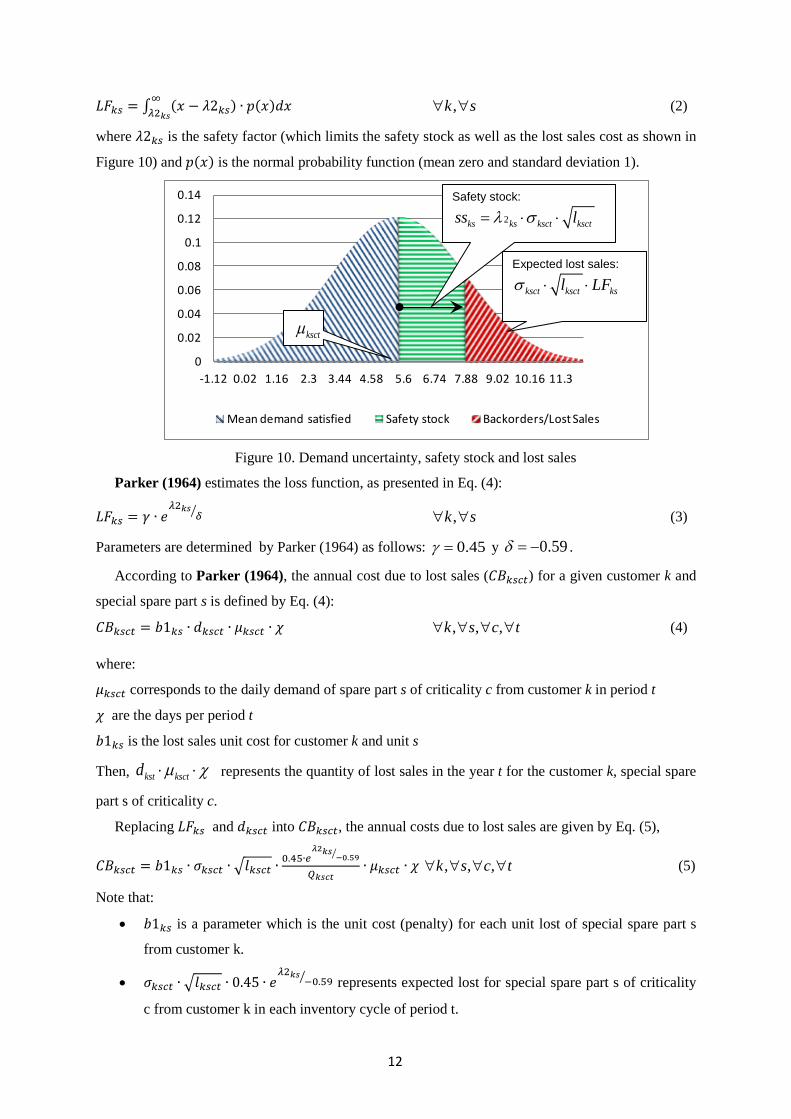
where 𝜆2𝑘𝑠 is the safety factor (which limits the safety stock as well as the lost sales cost as shown in
Figure 10) and 𝑝(𝑥) is the normal probability function (mean zero and standard deviation 1).
Figure 10. Demand uncertainty, safety stock and lost sales
Parker (1964) estimates the loss function, as presented in Eq. (4):
𝐿𝐹𝑘𝑠 = 𝛾 ∙ 𝑒𝜆2𝑘𝑠
𝛿� ,k s∀ ∀ (3)
Parameters are determined by Parker (1964) as follows: 0.45γ = y 0.59δ = − .
According to Parker (1964), the annual cost due to lost sales (𝐶𝐵𝑘𝑠𝑐𝑡) for a given customer k and
special spare part s is defined by Eq. (4):
𝐶𝐵𝑘𝑠𝑐𝑡 = 𝑏1𝑘𝑠 ∙ 𝑑𝑘𝑠𝑐𝑡 ∙ 𝜇𝑘𝑠𝑐𝑡 ∙ 𝜒
, , ,k s c t∀ ∀ ∀ ∀
(4) where:
𝜇𝑘𝑠𝑐𝑡 corresponds to the daily demand of spare part s of criticality c from customer k in period t
𝜒 are the days per period t
𝑏1𝑘𝑠 is the lost sales unit cost for customer k and unit s
Then, kst ksctd µ χ⋅ ⋅ represents the quantity of lost sales in the year t for the customer k, special spare
part s of criticality c.
Replacing 𝐿𝐹𝑘𝑠 and 𝑑𝑘𝑠𝑐𝑡 into 𝐶𝐵𝑘𝑠𝑐𝑡, the annual costs due to lost sales are given by Eq. (5),
𝐶𝐵𝑘𝑠𝑐𝑡 = 𝑏1𝑘𝑠 ∙ 𝜎𝑘𝑠𝑐𝑡 ∙ �𝑙𝑘𝑠𝑐𝑡 ∙0.45∙𝑒
𝜆2𝑘𝑠−0.59�
𝑄𝑘𝑠𝑐𝑡∙ 𝜇𝑘𝑠𝑐𝑡 ∙ 𝜒 , , ,k s c t∀ ∀ ∀ ∀
(5)
Note that:
• 𝑏1𝑘𝑠 is a parameter which is the unit cost (penalty) for each unit lost of special spare part s
from customer k.
• 𝜎𝑘𝑠𝑐𝑡 ∙ �𝑙𝑘𝑠𝑐𝑡 ∙ 0.45 ∙ 𝑒𝜆2𝑘𝑠
−0.59� represents expected lost for special spare part s of criticality
c from customer k in each inventory cycle of period t.
0
0.02
0.04
0.06
0.08
0.1
0.12
0.14
-1.12 0.02 1.16 2.3 3.44 4.58 5.6 6.74 7.88 9.02 10.16 11.3
Mean demand satisfied Safety stock Backorders/Lost Sales
ksctµ
Safety stock:
2ks ks ksct ksctss lλ σ ⋅⋅=
Expected lost sales:
ksct ksct ksl LFσ ⋅ ⋅
13
While:
• 𝜇𝑘𝑠𝑐𝑡∙𝜒𝑄𝑘𝑠𝑐𝑡
represents the number of cycles in the year.
Even though the safety factor 2ksλ is fixed (meaning that it is a parameter in the formulation),
since standard deviation during the net lead time is a variable (𝜎𝐿𝑇 = 𝜎𝑘𝑠𝑐𝑡 ∙ �𝑙𝑘𝑠𝑐𝑡), the cost of lost
sales is a variable as well. However, there is a difference between our model and the approach
proposed by Parker (1964) because the number of cycles per year is not given by 𝜇𝑘𝑠𝑐𝑡∙𝜒𝑄𝑘𝑠𝑐𝑡
, mainly for
two reasons:
• First, the order size 𝑄𝑘𝑠𝑐𝑡 is not a variable in our problem.
• Second, the inventory policy assumed is the periodic-review (order-up-to policy, base
stock level policy), which means that no equal amount is ordered in each cycle𝑄𝑘𝑠𝑐𝑡.
On the contrary, in each cycle the quantity ordered depends on the inventory position
at the time the order is placed.
Therefore, we propose to consider the number of cycles as follows: 𝜒
𝑡2𝑗𝑘𝑡∙ 𝑧𝑗𝑘𝑡
( ), , , ,psj k p s PS t∀ ∀ ∀ ∈ ∀
(6)
where χ indicates the number of days in the year,𝑡2𝑗𝑘𝑡indicates the total processing time (in days)
for a given standard spare part p in customer site k if the spare part is provided by warehouse j and
jktz is a binary variable which is one if warehouse j provides spare parts to customer k in period t.
This formula gives us the number of cycles per year.
Therefore, the annual cost of lost sales is given by Eq. (7).
𝐶𝐵𝑘𝑠𝑐𝑡 = 𝑏1𝑘𝑠 ∙ 𝜎𝑘𝑠𝑐𝑡 ∙ �𝑙𝑘𝑠𝑐𝑡 ∙ 0.45 ∙ 𝑒𝜆2𝑘𝑠
−0.59� ∙ 𝜒 ∙ ∑ 𝑧𝑗𝑘𝑡𝑡2𝑗𝑘𝑡𝑗 ( ), , , ,psk p s PS c t∀ ∀ ∈ ∀ ∀
(7)
5. Model formulation
5.1. MINLP multi-period problem
Given the supply chain structure presented in Figure 2, the following equations are applied to solve
the redesign problem. First, every customer k must be served by one warehouse j in each period t
according to Eq. (8).
∑ 𝑧𝑗𝑘𝑡𝑗 = 1
∀𝑘,∀𝑡
(8)
Regarding used repaired units, at most one repair work-shop j can be selected to repair unit s from
customer k in each period t, as shown in Eq. (9).
∑ 𝑣𝑗𝑘𝑠𝑡𝑗∈𝑆𝐶 ≤ 1
∀𝑘,∀𝑠,∀𝑡
(9)
As shown in Figure 5, tailor made units are directly supplied from factories to customers. Equation
(10) determines that only one factory i must produce and deliver tailor made spare parts s to each
customer k in period t.
14
∑ 𝑢𝑖𝑘𝑠𝑡𝑖 = 1 , ,k s t∀ ∀ ∀ (10)
Equation (11) determines that standard spare part p can be delivered from factory i to warehouse j
in period t if the warehouse was installed and never uninstalled in period t or before.
𝑥𝑖𝑗𝑝𝑡 ≤ ∑ 𝑦𝑗𝑡′𝑡′≤𝑡 − ∑ 𝑦𝑗𝑡′𝑢𝑡′≤𝑡
, , ,i j p t∀ ∀ ∀ ∀ (11)
Equation (12) determines that standard spare part p can be delivered from factory i to warehouse j
in period t if the factory i was installed and never uninstalled in period t or before.
𝑥𝑖𝑗𝑝𝑡 ≤ ∑ 𝑤𝑖𝑡′𝑡′≤𝑡 − ∑ 𝑤𝑖𝑡′𝑢𝑡′≤𝑡
, , ,i j p t∀ ∀ ∀ ∀ (12)
Equation (13) determines that tailor made unit s can be delivered from factory i to end customer k
in period t if the factory i was installed and never uninstalled in period t or before.
𝑢𝑖𝑘𝑠𝑡 ≤ ∑ 𝑤𝑖𝑡′𝑡′≤𝑡 − ∑ 𝑤𝑖𝑡′𝑢𝑡′≤𝑡
( ), , ,ksi k s KT t∀ ∀ ∈ ∀ (13)
According to Eq. (14), warehouse j in period t can be expanded if the warehouse was previously
installed.
𝑦𝑗𝑡𝑒 ≤ ∑ 𝑦𝑗𝑡′𝑡′≤𝑡 ,j t∀ ∀ (14)
Warehouse j in period t can be eliminated or uninstalled in Eq. (15) if the warehouse was
previously installed.
𝑦𝑗𝑡𝑢 ≤ ∑ 𝑦𝑗𝑡′𝑡′≤𝑡
,j t∀ ∀
(15)
Equation(16) establishes that factory i in period t can be expanded if the factory was previously
installed.
𝑤𝑖𝑡𝑒 ≤ ∑ 𝑤𝑖𝑡′𝑡′≤𝑡 ,i t∀ ∀ (16)
According to Eq. (17), factory i in period t can be eliminated or uninstalled if that factory was
previously installed.
𝑤𝑖𝑡𝑢 ≤ ∑ 𝑤𝑖𝑡′𝑡′≤𝑡
,i t∀ ∀
(17)
As shown in Eq. (18), a customer k can be served by a warehouse j in period t if that warehouse
has been previously installed, and was never uninstalled before and during that period.
𝑧𝑗𝑘𝑡 ≤ ∑ 𝑦𝑗𝑡′𝑡′≤𝑡 − ∑ 𝑦𝑗𝑡′𝑢𝑡′≤𝑡
, ,j k t∀ ∀ ∀
(18)
Similar to the previous constraint, Eq. (19)allows that a repair work-shop serves a customer k with
used units s in period t if that work-shop has been previously installed, and was never uninstalled
before and during that period.
𝑣𝑗𝑘𝑠𝑡 ≤ ∑ 𝑦𝑗𝑡′𝑡′≤𝑡 − ∑ 𝑦𝑗𝑡′𝑢𝑡′≤𝑡 ∀𝑗 ∈ 𝑆𝐶,∀𝑘,∀𝑠,∀𝑡
(19)
As it was previously mentioned, demand of units due to failure rate can be satisfied with new and
repaired used units. Constraint (20) establishes that total mean demand ksctµ must be satisfied either
with new ( newijkptµ ) or with used parts ( used
jkstµ ).
∑ ∑ 𝜇𝑖𝑗𝑘𝑝𝑡𝑛𝑒𝑤𝑗𝑖 + ∑ ∑ ∑ 𝜇𝑗𝑘𝑠𝑡𝑢𝑠𝑒𝑑
𝑗𝑠∈�𝐾𝑆𝐶𝑘𝑠𝑐∩𝑃𝑆𝑝𝑠∩𝐶𝑇𝑘𝑠�𝑠∉𝐾𝑇𝑘𝑠
𝑗∈𝑆𝐶 = ∑ ∑ 𝜇𝑘𝑠𝑐𝑡𝑐∈𝐾𝑆𝐶𝑘𝑠𝑐𝑠∈𝑃𝑆𝑝𝑠𝑠∉𝐾𝑇𝑘𝑠
, ,k p t∀ ∀ ∀ (20)
15
In case the customer does not allow repaired parts, Eq. (21) establishes that the total demand must
be satisfied with new units. Variable newijkptµ is needed in order to determine from which factory i and
warehouse j demand of customer k in period t is satisfied.
∑ ∑ 𝜇𝑖𝑗𝑘𝑝𝑡𝑛𝑒𝑤𝑗𝑖 = ∑ ∑ 𝜇𝑘𝑠𝑐𝑡𝑐∈𝐾𝑆𝐶𝑘𝑠𝑐𝑠∈𝑃𝑆𝑝𝑠
𝑠∉(𝐾𝑇𝑘𝑠∪𝐶𝑇𝑘𝑠) , ,k p t∀ ∀ ∀ (21)
In the case of tailor made parts, Eq. (22)is applied. The total demand for tailor made parts must be
satisfied either with new or used units. The main difference between standard and tailor made units
regarding model formulation is that tailor made spare parts are delivered directly from plants, while
standard spare parts are delivered from warehouses.
∑ 𝜏𝑖𝑘𝑠𝑡𝑛𝑒𝑤𝑖 + ∑ 𝜏𝑗𝑘𝑠𝑡𝑢𝑠𝑒𝑑
𝑗𝜖𝑆𝐶 = ∑ 𝜇𝑘𝑠𝑐𝑡𝑐∈𝐾𝑆𝐶𝑘𝑠𝑐
( , ) ,ksk s KT t∀ ∈ ∀
(22)
In the case that the customer does not allow repaired spare parts to satisfy tailor made units
demand, Eq. (23) determines that all units expected to fail are replaced by new units.
∑ 𝜏𝑖𝑘𝑠𝑡𝑛𝑒𝑤𝑖 = ∑ 𝜇𝑘𝑠𝑐𝑡𝑐∈𝐾𝑆𝐶𝑘𝑠𝑐 ∀(𝑘, 𝑠) ∉ (𝐾𝑇𝑘𝑠 ∪ 𝐶𝑇𝑘𝑠) (23)
Eq. (24)is a bilinear inequality that represents an upper bound for variable newijkptµ , where binary
variables ijptx and jktz represent the selected links in the supply chain. The first variable is one if
factory i produces and delivers standard unit p to warehouse j in period t, while the second is one if
warehouse j delivers units to end customer k in period t. Only if both variables are positive, then
demand of customer k can be satisfied with new units.
𝜇𝑖𝑗𝑘𝑝𝑡𝑛𝑒𝑤 ≤ ∑ ∑ 𝜇𝑘𝑠𝑐𝑡 ∙ 𝑥𝑖𝑗𝑝𝑡 ∙ 𝑧𝑗𝑘𝑡𝑐∈𝐾𝑆𝐶𝑘𝑠𝑐𝑠∈𝑃𝑆𝑝𝑠𝑠∉𝐾𝑇𝑘𝑠
, , , ,i j k p t∀ ∀ ∀ ∀ ∀ (24)
Eq. (25) has the same purpose as Eq. (24), it is an upper bound for mean demand level in each
node of the supply chain according to the selected links, in this case, for tailor made units.
𝜏𝑖𝑘𝑠𝑡𝑛𝑒𝑤 ≤ ∑ 𝜇𝑘𝑠𝑐𝑡𝑐∈𝐾𝑆𝐶𝑘𝑠𝑐 ∙ 𝑢𝑖𝑘𝑠𝑡 , ( , ) ,ksi k s KT t∀ ∀ ∈ ∀ (25)
Eq. (26) determines that if repair workshop j (also warehouse j) is selected to repair special unit s
of end customer k in period t, given by binary variable 𝑣𝑗𝑘𝑠𝑡, then the total amount of used spare parts
required is given by the expected demand level ksctµ multiplied by the repairing probability ksrp .
𝜇𝑗𝑘𝑝𝑡𝑢𝑠𝑒𝑑 = ∑ ∑ 𝜇𝑘𝑠𝑐𝑡 ∙ 𝑣𝑗𝑘𝑠𝑡 ∙ 𝑟𝑝𝑘𝑠𝑠∈�𝑃𝑆𝑝𝑠∩𝐶𝑇𝑘𝑠�𝑠∉𝐾𝑇𝑘𝑠
𝑐∈𝐾𝑆𝐶𝑘𝑠𝑐
, , ,j SC k p t∀ ∈ ∀ ∀ ∀
(26)
Some customers might also allow tailor made spare parts to be repaired. If that is the case, the total
amount of units satisfied with used repaired units is given by the total demand due to failure rate
multiplied by repairing probability. This constraint is given in Eq. (27).
𝜏𝑗𝑘𝑠𝑡𝑢𝑠𝑒𝑑 = ∑ 𝜇𝑘𝑠𝑐𝑡 ∙ 𝑣𝑗𝑘𝑠𝑡 ∙ 𝑟𝑝𝑘𝑠𝑐∈𝐾𝑆𝐶𝑘𝑠𝑐 , ( , ) ,ksj SC k s KT t∀ ∈ ∀ ∈ ∀ (27)
The net lead time of warehouse j, standard unit p in period t is determined in Eq. (28). As
mentioned, a safety stock level is defined in order to prevent a shortage in stock due to uncertain
16
demand increase. As explained in section 4.2, this safety stock level is calculated according to the net
lead time determined in Eq. (28).
𝑛𝑗𝑝𝑡 ≥ �𝑆𝐼𝑖𝑝 + 𝑡1𝑖𝑗𝑝� ∙ 𝑥𝑖𝑗𝑝𝑡 − 𝑠𝑗𝑝𝑡 , , ,i j p t∀ ∀ ∀ ∀ (28)
Net lead time of tailor made unit s and customer k in period t is calculated in Eq. (29). Similarly,
the net lead time of special spare parts s for each k in period t is determined in Eq. (30). While Eq.
(29) is linear, Eq. (30) involves a bilinear product of variable jpts by jktz .
𝑚𝑘𝑠𝑐𝑡 ≥ (𝐺𝐼𝑖𝑠 + 𝑡3𝑖𝑘𝑠) ∙ 𝑢𝑖𝑘𝑠𝑡 − 𝑅𝑘𝑠𝑐 ( ), ( , , ) ,ksc ksi k s c KSC KT t∀ ∀ ∈ ∩ ∀ (29)
𝑙𝑘𝑠𝑐𝑡 ≥ ∑ 𝑠𝑗𝑝𝑡 ∙ 𝑧𝑗𝑘𝑡𝑗 + ∑ 𝑡2𝑗𝑘𝑝 ∙ 𝑧𝑗𝑘𝑡𝑗 − 𝑅𝑘𝑠𝑐 , ( , , ) , ( , , ) ,ksc ksi k s c KSC k s c KT t∀ ∀ ∈ ∀ ∉ ∀ (30)
The safety stock of standard spare part p in warehouse j for each period t is determined by Eq.
(31). This variable is calculated multiplying the safety factor jpλ , standard deviation 𝜎𝑘𝑠𝑐𝑡 and the
square root of the net lead time of warehouse j, standard spare part p in period t.
𝑠𝑠𝑗𝑝𝑡 = 𝜆𝑗𝑝�∑ ∑ ∑ 𝑛𝑗𝑝𝑡 ∙ 𝑧𝑗𝑘𝑡 ∙ 𝜎𝑘𝑠𝑐𝑡2𝑐∈𝐾𝑆𝐶𝑘𝑠𝑐𝑠∈𝑃𝑆𝑝𝑠𝑠∉𝐾𝑇𝑘𝑠
𝑘 , ,j p t∀ ∀ ∀ (31)
As shown in Fig. 3, the capacity profile evolves during the planning horizon according to
investment decisions. In the case of warehouses, this variable is established in Eq. (32) as the capacity
level in the previous period, plus the expansion jtce in the present period minus the uninstalled
capacity jtuc in period t. It should be noted that expansions and elimination of warehouses cannot be
made simultaneously as shown later in Eq. (39). Note that when t=1, 1jtq − = jIC .
𝑞𝑗𝑡 = 𝑞𝑗𝑡−1 + 𝑐𝑒𝑗𝑡 − 𝑢𝑐𝑗𝑡 0, , where j jj t q IC∀ ∀ = (32)
Equation (33) determines that the maximum capacity expansion of warehouse j in each period t,
jtce , is given by UPjQDC when warehouse j is installed ( 1jty = ) or expanded ( 1e
jty = ).
𝑐𝑒𝑗𝑡 ≤ 𝑄𝐷𝐶𝑗𝑈𝑃 ∙ �𝑦𝑗𝑡 + 𝑦𝑗𝑡𝑒 � ,j t∀ ∀ (33)
In case a warehouse is already installed in period 1, Eq. (34) determines that the maximum
capacity expansion of warehouse j, jtce , is given by UPjQDC when warehouse j is expanded ( 1e
jty =
).
𝑐𝑒𝑗𝑡 ≤ 𝑄𝐷𝐶𝑗𝑈𝑃 ∙ 𝑦𝑗𝑡𝑒 , 1j JF t∀ ∈ = (34)
Maximum capacity in each period for warehouse j is given by Eq. (35). This upper bound is given
by the initial capacity, jIC , plus the maximum capacity expansion per period, UPjQDC , multiplied by
the number of periods t. Note also that if this warehouse is eliminated ( 1ujty = ), then capacity
0jtq = .
𝑞𝑗𝑡 ≤ �𝑄𝐷𝐶𝑗𝑈𝑃 ∙ 𝑡 + 𝐼𝐶𝑗� ∙ �1 − 𝑦𝑗𝑡𝑢� ,j t∀ ∀ (35)
17
Similarly, Eq. (36) determines an upper bound for the capacity that is uninstalled if warehouse j is
eliminated.
𝑢𝑐𝑗𝑡 ≤ �𝑄𝐷𝐶𝑗𝑈𝑃 ∙ 𝑡 + 𝐼𝐶𝑗� ∙ 𝑦𝑗𝑡𝑢 ,j t∀ ∀ (36)
According to Eq. (37), warehouse j can be installed only once in the time horizon.
∑ 𝑦𝑗𝑡𝑡 ≤ 1 j∀ (37)
Also, warehouse j can be uninstalled only once in the time horizon determined by Eq. (38).
∑ 𝑦𝑗𝑡𝑢𝑡 ≤ 1
j∀
(38)
Equations(39)and (40) establish that a warehouse j cannot be installed, uninstalled and expanded in
the same period. Only one decision at a time can be made. This constraint is applied for all
warehouses j that are not installed in the supply chain in period 1 (Eq. (39)), or for warehouses j in
any period greater than 1 (Eq. (40)).
𝑦𝑗𝑡 + 𝑦𝑗𝑡𝑢 + 𝑦𝑗𝑡𝑒 ≤ 1 , 1j JF t∀ ∉ =
(39)
𝑦𝑗𝑡 + 𝑦𝑗𝑡𝑢 + 𝑦𝑗𝑡𝑒 ≤ 1 , 1j t∀ ∀ >
(40)
Equation (41) establishes that a warehouse j cannot be uninstalled and expanded in period 1 if the
warehouse is already installed in the supply chain ( j JF∈ ). Only one decision at a time can be
made.
𝑦𝑗𝑡𝑢 + 𝑦𝑗𝑡𝑒 ≤ 1 , 1j JF t∀ ∈ = (41)
Capacity of factory i is defined in Eq. (42) as the capacity in the previous periods plus the capacity
expansion minus capacity elimination in the same period. Note that for t=1,𝑞𝑓𝑖𝑡−1 = 𝐼𝐶𝐹𝑖.
𝑞𝑓𝑖𝑡 = 𝑞𝑓𝑖𝑡−1 + 𝑐𝑒𝑓𝑖𝑡 − 𝑢𝑐𝑓𝑖𝑡 0, , where i ii t qf ICF∀ ∀ = (42)
Equation (43) determines that the maximum capacity expansion of factory i in each period t, itcef ,
is given by UPiQP when factory i is installed ( 1itw = ) or expanded ( 1e
itw = ).
𝑐𝑒𝑓𝑖𝑡 ≤ 𝑄𝑃𝑖𝑈𝑃 ∙ (𝑤𝑖𝑡 + 𝑤𝑖𝑡𝑒 ) ,i t∀ ∀ (43)
If the factory is fixed at the beginning of the horizon planning ( i IF∀ ∈ ), Eq. (44) determines that
the maximum capacity expansion of factory i in period 1, 1icef , is given by UPiQP only if i is
expanded in that period ( 1eitw = ).
𝑐𝑒𝑓𝑖𝑡 ≤ 𝑄𝑃𝑖𝑈𝑃 ∙ 𝑤𝑖𝑡𝑒 , 1i IF t∀ ∈ = (44)
Eq. (45) defines the maximum capacity in each period for factory i. This upper bound is given by
the initial capacity, iICF , plus the maximum capacity expansion per period, UPiQP , multiplied by the
number of periods t. Note also that if this factory is eliminated ( 1uitw = ), then capacity itqf is set to 0.
𝑞𝑓𝑖𝑡 ≤ �𝑄𝑃𝑖𝑈𝑃 ∙ 𝑡 + 𝐼𝐶𝐹𝑖� ∙ (1 −𝑤𝑖𝑡𝑢) ,i t∀ ∀ (45)
18
Similarly, Eq. (46) determines an upper bound for the capacity that is uninstalled when factory i is
eliminated.
𝑢𝑐𝑓𝑖𝑡 ≤ �𝑄𝑃𝑖𝑈𝑃 ∙ 𝑡 + 𝐼𝐶𝐹𝑖� ∙ 𝑤𝑖𝑡𝑢 ,i t∀ ∀ (46)
Factory i can be installed only once in the time horizon given by Eq. (47).
∑ 𝑤𝑖𝑡𝑡 ≤ 1 i∀ (47)
Also, factory i can be uninstalled only once in the time horizon according to Eq. (48).
∑ 𝑤𝑖𝑡𝑢𝑡 ≤ 1
i∀
(48)
Equations (49) and (50) establish that only one decision regarding installation, elimination or
expansion can be made in each period for a factory i. This constraint is applied for all factories i
which are not installed in the supply chain in period 1 (Eq. (49)) or for any factory i in any period
greater than 1 (Eq. (50)).
𝑤𝑖𝑡 + 𝑤𝑖𝑡𝑢 +𝑤𝑖𝑡𝑒 ≤ 1 , 1i IF t∀ ∉ =
(49)
𝑤𝑖𝑡 + 𝑤𝑖𝑡𝑢 +𝑤𝑖𝑡𝑒 ≤ 1 , 1i t∀ ∀ >
(50)
Equation (51) establishes that a factory i that is already installed in the supply chain ( i IF∈ ) can
be uninstalled or expanded in period 1 but only one of these decisions can be made.
𝑤𝑖𝑡𝑢 + 𝑤𝑖𝑡𝑒 ≤ 1 , 1i IF t∀ ∈ = (51)
Equation (52) determines that the maximum amount of stock-keeping units (SKU) in a warehouse
j in period t cannot exceed the capacity jtq which is the total amount of units that can be stored in the
warehouse j. This amount is calculated considering both pipeline inventory and safety stock. In order
to calculate the amount of new units in stock due to mean level inventory (Little, 1961), the daily
demand newijkptµ is multiplied by the processing time 1ijpt in warehouse j if the unit is delivered from
factory i. This amount is then multiplied by a size parameter pβ indicating the portion of stock
capacity a given standard unit p uses when it is stored. Similarly, in the case of used spare parts, the
amount of them in stock is calculated as the product of the daily demand satisfied with used spare
parts ( usedjkptµ in the case of standard spare parts and used
jkstτ in the case of tailor made units) multiplied
by the time they are stored in average in the warehouse before they go back to the customers, jptsu
and jsttu , respectively. Both quantities are then multiplied by the corresponding size factors ( pβ in
the case of standard units and 2sβ for tailor made). The portion of capacity used by the safety stock is
calculated in the last term multiplying the safety stock jptss (in units of spare parts) by the size factor
pβ .
∑ ∑ �∑ 𝜇𝑖𝑗𝑘𝑝𝑡𝑛𝑒𝑤𝑖 ∙ 𝑡1𝑖𝑗𝑝 + 𝜇𝑗𝑘𝑝𝑡𝑢𝑠𝑒𝑑 ∙ 𝑡𝑠𝑢𝑗𝑝�𝑝𝑘 ∙ 𝛽𝑝 +∑ ∑ 𝜏𝑗𝑘𝑠𝑡𝑢𝑠𝑒𝑑
𝑠 ∈(𝐾𝑇𝑘𝑠∩𝐶𝑇𝑘𝑠)𝑘 ∙ 𝑡𝑡𝑢𝑗𝑠 ∙ 𝛽2𝑠 + ∑ 𝑠𝑠𝑗𝑝𝑡𝑝 ∙
𝛽𝑝 ≤ 𝑞𝑗𝑡
,j t∀ ∀
(52)
19
Eq. (53)determines that daily demand satisfied with new units newijkptµ multiplied by capacity factor
pα cannot exceed the capacity of this factory.
∑ ∑ ∑ 𝜇𝑖𝑗𝑘𝑝𝑡𝑛𝑒𝑤𝑗𝑝𝑘 ∙ 𝛼𝑝 ≤ 𝑞𝑓𝑖𝑡 ,i t∀ ∀ (53)
The following equations, from Eq.(54) to (71), introduce the different cost terms used in the
objective function.
Equation (54) indicates total investment cost in new warehouses for each period, tTI . It should be
noted that if a warehouse is already installed ( j FJ∈ ) at the beginning of the horizon planning then
fjis zero. 𝑇𝐼𝑡 = ∑ 𝑓𝑗 ∙ 𝑦𝑗𝑡𝑗
t∀ (54)
Similarly, Eq.(55) indicates total investment cost per period in new factories, tTPI . If a factory is
already installed ( i FI∈ ) at the beginning of the horizon planning then fpi is zero. 𝑇𝑃𝐼𝑡 = ∑ 𝑓𝑝𝑖 ∙ 𝑤𝑖𝑡𝑖
t∀ (55)
Total operational fixed costs tTOF are given by Eq. (56). This fixed cost jofc must be paid while
a warehouse is installed, from the moment it is installed until it is eliminated. Therefore, if a
warehouse was uninstalled in any previous or present period this cost is no longer paid. This cost will
prevent to keep opened a warehouse which is not used.
𝑇𝑂𝐹𝑡 = ∑ 𝑜𝑓𝑐𝑗 ∙ �∑ 𝑦𝑗𝑡′𝑡′≤𝑡 − ∑ 𝑦𝑗𝑡′𝑢𝑡′≤𝑡 �𝑗 t∀ (56)
Similar to the case of warehouses, there is an operational fixed cost for factories. The total costs
tTPF is considered in Eq. (57). This fixed cost ipfc must be paid while the factory is installed, from
the moment it is installed until it is eliminated. The aim of this cost is to keep opened just factories
that are in used.
𝑇𝑃𝐹𝑡 = ∑ 𝑝𝑓𝑐𝑖 ∙ (∑ 𝑤𝑖𝑡′𝑡′≤𝑡 − ∑ 𝑤𝑖𝑡′𝑢𝑡′≤𝑡 )𝑖 t∀ (57)
Total investment expansion costs in each period tTE are determined in Eq. (58). This investment
cost jec must be paid whenever an expansion is decided ( 1ejty = ).
𝑇𝐸𝑡 = ∑ 𝑒𝑐𝑗 ∙ 𝑦𝑗𝑡𝑒𝑗 t∀ (58)
Total investment costs in each period for expansion of factories tTEP are determined in Eq. (59).
This investment cost 𝑒𝑐𝑝𝑖is considered in the period the expansion is decided ( 1eitw = ).
𝑇𝐸𝑃𝑡 = ∑ 𝑒𝑐𝑝𝑖 ∙ 𝑤𝑖𝑡𝑒𝑖 t∀ (59)
If a warehouse is uninstalled, then the fixed costs juc have to be paid. Total elimination cost in
each period ( tTU ) is calculated in Eq. (60).
𝑇𝑈𝑡 = ∑ 𝑢𝑐𝑗 ∙ 𝑦𝑗𝑡𝑢𝑗 t∀ (60)
20
As for warehouses, when a factory is uninstalled there is a fixed cost iucp to be paid. Total
elimination cost of factories in each period ( tTUP ) is calculated in Eq. (61).
𝑇𝑈𝑃𝑡 = ∑ 𝑢𝑐𝑝𝑖 ∙ 𝑤𝑖𝑡𝑢𝑖 t∀ (61)
Equation (62) determines the amount of total variable costs per period in the warehouses. It is
calculated as the product of the unit variable cost𝑔𝑗, the daily demand𝜇𝑖𝑗𝑘𝑝𝑡𝑛𝑒𝑤 and the number of days
per period 𝜒.
𝑇𝑂𝑉𝑡 = ∑ ∑ ∑ ∑ 𝑔𝑗 ∙ 𝜇𝑖𝑗𝑘𝑝𝑡𝑛𝑒𝑤 ∙ 𝜒𝑝𝑘𝑗𝑖 t∀ (62)
Similarly, Eq. (63) determines the amount of total variable costs per period in factories. It is
calculated as the product of the unit variable cost igp , the daily demand newijkptµ and the number of
days per period χ .
𝑇𝑃𝑉𝑡 = ∑ ∑ ∑ ∑ 𝑔𝑝𝑖 ∙ 𝜇𝑖𝑗𝑘𝑝𝑡𝑛𝑒𝑤 ∙ 𝜒𝑝𝑘𝑗𝑖 t∀ (63)
Repair cost in each period t, is given by Eq. (64). This cost is determined for standard and tailor
made units.
𝑇𝑅𝑡 = ∑ ∑ ∑ 𝑔𝑟𝑗𝑝 ∙ 𝜇𝑗𝑘𝑝𝑡𝑢𝑠𝑒𝑑 ∙ 𝜒𝑝𝑘𝑗𝜖𝑆𝐶 + ∑ ∑ ∑ 𝑔𝑟′𝑗𝑠 ∙ 𝜏𝑗𝑘𝑠𝑡𝑢𝑠𝑒𝑑 ∙ 𝜒𝑠𝜖𝐾𝑇𝑘𝑠𝑘𝑗𝜖𝑆𝐶 t∀ (64)
Transportation costs from factories are determined in Eq. (65). Unit transportation cost from
factories i to warehouses j 1ijc are multiplied by standard daily demand newijkptµ and the number of days
χ . In the case of tailor made spare parts, unit transportation cost from factories i to customer site k
3ikc is multiplied by the daily demand newikstτ and days per period χ .
𝑇𝑇𝐹𝑡 = ∑ ∑ ∑ ∑ 𝑐1𝑖𝑗 ∙ 𝜇𝑖𝑗𝑘𝑝𝑡𝑛𝑒𝑤 ∙ 𝜒𝑝𝑘𝑗𝜖𝑆𝐶𝑖 + ∑ ∑ ∑ 𝑐3𝑖𝑘 ∙ 𝜏𝑖𝑘𝑠𝑡𝑛𝑒𝑤 ∙ 𝜒𝑠𝜖𝐾𝑇𝑘𝑠𝑘𝑖 t∀ (65)
Transportation costs from warehouses are determined in Eq. (66). Unit transportation cost from
warehouses j to customers k 2 jkc are multiplied by standard daily demand newijkptµ and the number of
days χ . In the case of repaired standard and tailor made spare parts, the same unit transportation cost
is multiplied by 2 to consider the double route, from customers to workshops, and from workshops to
customers. This cost is multiplied by the daily demand satisfied with repaired used spare parts ( usedjkstτ
in the case of tailor made and usedjkptµ in the case of standard spare parts) and by the days per period χ .
𝑇𝑇𝑊𝑡 = ∑ ∑ ∑ ∑ 𝑐2𝑗𝑘 ∙ 𝜇𝑖𝑗𝑘𝑝𝑡𝑛𝑒𝑤 ∙ 𝜒𝑝𝑘𝑗𝑖 + ∑ ∑ 2 ∙ 𝑐2𝑗𝑘 ∙ 𝜒�∑ 𝜇𝑗𝑘𝑝𝑡𝑢𝑠𝑒𝑑 + ∑ 𝜏𝑗𝑘𝑠𝑡𝑢𝑠𝑒𝑑𝑠𝜖𝐾𝑇𝑘𝑠𝑝 �𝑘𝑗𝜖𝑆𝐶 t∀ (66)
Mean inventory costs in warehouses are calculated in Eq. (67) as the unit inventory cost per day
1 jpθ multiplied by the daily demand newijkptµ and the processing time 1ijpt .
𝑇𝑃𝑊𝑡 = ∑ ∑ ∑ ∑ 𝜃1𝑗𝑝 ∙ 𝜇𝑖𝑗𝑘𝑝𝑡𝑛𝑒𝑤 ∙ 𝑡1𝑖𝑗𝑝𝑝𝑘𝑗𝑖 t∀ (67)
21
Similarly, mean inventory costs at customer sites are calculated in Eq. (68)for special and tailor
made units. This cost is determined multiplying the unit inventory cost per day, 2kpθ and 𝜃3𝑘𝑝,
multiplied by the daily demand, newijkptµ and𝜏𝑖𝑘𝑠𝑡𝑛𝑒𝑤, and the processing time, 2 jkpt and 𝑡3𝑖𝑘𝑠, respectively.
𝑇𝑃𝐶𝑡 = ∑ ∑ ∑ ∑ 𝜃2𝑘𝑝 ∙ 𝜇𝑖𝑗𝑘𝑝𝑡𝑛𝑒𝑤 ∙ 𝑡2𝑗𝑘𝑝𝑝𝑘𝑗𝑖 + ∑ ∑ ∑ 𝜃3𝑘𝑝 ∙ 𝜏𝑖𝑘𝑠𝑡𝑛𝑒𝑤 ∙ 𝑡3𝑖𝑘𝑠𝑠𝜖𝐾𝑇𝑘𝑠𝑘𝑖 t∀ (68)
Safety stock costs are determined by Eq. (69). The first term indicates safety stock cost at
warehouses for standard units, the second term calculates safety stock cost at customer sites for
standard units, while the third term determines the safety stock cost at customer sites for tailor made
parts.
𝑇𝑆𝑆𝑡 =
∑ ∑ ℎ1𝑗𝑝 ∙ 𝑠𝑠𝑗𝑝𝑡𝑝𝑗 + ∑ ∑ ∑ ℎ2𝑘 ∙ 𝜆2𝑘𝑠 ∙ 𝜎𝑘𝑠𝑐𝑡 ∙ �𝑙𝑘𝑠𝑐𝑡𝑐𝜖𝐾𝑆𝐶𝑘𝑠𝑐𝑠∉𝐾𝑇𝑘𝑠𝑘 + ∑ ∑ ∑ ℎ2𝑘 ∙𝑐𝜖𝐾𝑆𝐶𝑘𝑠𝑐𝑠𝜖𝐾𝑇𝑘𝑠𝑘
𝜆2𝑘𝑠 ∙ 𝜎𝑘𝑠𝑐𝑡 ∙ �𝑚𝑘𝑠𝑐𝑡 t∀ (69)
As it was explained in Section 3.5, lost sales costs are also included in the objective function.
Equation (70) determines the lost sales cost for standard parts while Eq. (71) calculates this cost for
tailor made units.
𝑇𝐵𝑇𝑡 = ∑ ∑ ∑ 𝑏1𝑘𝑠 ∙ 0.45 ∙ 𝜎𝑘𝑠𝑐𝑡 ∙ �𝑙𝑘𝑠𝑐𝑡 ∙ 𝑒𝜆2𝑘𝑠
−0.59�𝑐𝜖𝐾𝑆𝐶𝑘𝑠𝑐𝑠∉𝐾𝑇𝑘𝑠𝑘 ∙ 𝜒 ∙ ∑ 𝑧𝑗𝑘𝑡
𝑡2𝑗𝑘𝑠𝑗 t∀ (70)
𝑇𝐵𝑆𝑡 = ∑ ∑ ∑ 𝑏1𝑘𝑠 ∙ 0.45 ∙ 𝜎𝑘𝑠𝑐𝑡 ∙ �𝑚𝑘𝑠𝑐𝑡 ∙ 𝑒𝜆2𝑘𝑠
−0.59�𝑐𝜖𝐾𝑆𝐶𝑘𝑠𝑐𝑠∈𝐾𝑇𝑘𝑠𝑘 ∙ 𝜒 ∙ ∑ 𝑢𝑖𝑘𝑠𝑡
𝑡3𝑖𝑘𝑠𝑖 t∀ (71)
Including all these costs, the objective function is given by Eq. (72).
Min C
𝐶 = ∑ 𝑇𝐼𝑡+𝑇𝑃𝐼𝑡+𝑇𝑂𝐹𝑡+𝑇𝑃𝐹𝑡+𝑇𝐸𝑡+𝑇𝐸𝑃𝑡+𝑇𝑈𝑡+𝑇𝑈𝑃𝑡+𝑇𝑂𝑉𝑡+𝑇𝑃𝑉𝑡+𝑇𝑅𝑡+𝑇𝑇𝐹𝑡+𝑇𝑇𝑊𝑡+𝑇𝑃𝑊𝑡+𝑇𝑃𝐶𝑡+𝑇𝑆𝑆𝑡+𝑇𝐵𝑇𝑡+𝑇𝐵𝑆𝑡(1+𝑖𝑟)𝑡𝑡 (72)
Finally, the original problem P0 is given by Eqs. (8)–(72). This is an MINLP formulation due to
bilinear terms in Eqs. (24)and(30), and square root terms in Eqs.(31) and (69)–(71).
5.2. Problem reformulation as an MILP
In this section, non-linear equations from problem P0 are transformed to obtain a linear relaxation.
In the case of bilinear term (products of binaries or continuous times binary variable) exact
reformulations are proposed, while a linear approximation is used for the square root terms which
yields a lower bound of the original functions.
Considering that 𝑥𝑖𝑗𝑝𝑡 and 𝑧𝑗𝑘𝑡 are binary variables, the nonlinear term appearing in Eq. (24) can
be replaced by a new variable 𝑥𝑧𝑖𝑗𝑘𝑝𝑡 adding the following equations:
𝑥𝑧𝑖𝑗𝑘𝑝𝑡 ≤ 𝑥𝑖𝑗𝑝𝑡 , , , ,i j k p t∀ ∀ ∀ ∀ ∀ (73)
𝑥𝑧𝑖𝑗𝑘𝑝𝑡 ≤ 𝑧𝑗𝑘𝑡 , , , ,i j k p t∀ ∀ ∀ ∀ ∀ (74)
𝑥𝑧𝑖𝑗𝑘𝑝𝑡 ≥ 𝑧𝑗𝑘𝑡 + 𝑥𝑖𝑗𝑝𝑡 − 1 , , , ,i j k p t∀ ∀ ∀ ∀ ∀ (75)
22
where0 ≤ 𝑥𝑧𝑖𝑗𝑘𝑝𝑡 ≤ 1
Equation (24) can be now replaced by:
𝜇𝑖𝑗𝑘𝑝𝑡𝑛𝑒𝑤 ≤ ∑ ∑ 𝜇𝑘𝑠𝑐𝑡 ∙ 𝑥𝑧𝑖𝑗𝑘𝑝𝑡𝑐∈𝐾𝑆𝐶𝑘𝑠𝑐𝑠∈𝑃𝑆𝑝𝑠𝑠∉𝐶𝑇𝑘𝑠
, , , ,i j k p t∀ ∀ ∀ ∀ ∀ (76)
Similarly, the bilinear term from Eq. (30) involving continuous variable 𝑠𝑗𝑝𝑡 and binary variable
𝑧𝑗𝑘𝑡, can be replaced by a new variable 𝑠𝑧𝑗𝑘𝑝𝑡. Auxiliary variable 𝑠𝑧1𝑗𝑘𝑝𝑡 is also introduced in the
formulation, as follows:
𝑠𝑧𝑗𝑘𝑝𝑡 ≤ 𝑧𝑗𝑘𝑡 ∙ 𝑠𝑗𝑝𝑡𝑈𝑃 , , ,j k p t∀ ∀ ∀ ∀ (77)
𝑠𝑧𝑗𝑘𝑝𝑡 ≤ �1 − 𝑧𝑗𝑘𝑡� ∙ 𝑠𝑗𝑝𝑡𝑈𝑃 , , ,j k p t∀ ∀ ∀ ∀ (78)
𝑠𝑗𝑝𝑡 ≥ 𝑠𝑧𝑗𝑘𝑝𝑡 + 𝑠𝑧1𝑗𝑘𝑝𝑡 , , ,j k p t∀ ∀ ∀ ∀ (79)
Eq. (30) is now replaced by (52):
𝑙𝑘𝑠𝑐𝑡 ≥ ∑ 𝑠𝑧𝑗𝑘𝑝𝑡𝑗 + ∑ 𝑡2𝑗𝑘𝑝 ∙ 𝑧𝑗𝑘𝑡𝑗 − 𝑅𝑘𝑠𝑐 , ( , , ) , ( , ) ,ksc ksi k s c KSC k s KT t∀ ∀ ∈ ∀ ∉ ∀ (80)
In the case of Eq. (31), since a bilinear term and a square root is involved, then the linearization is
given in two steps. First the bilinear term of 𝑧𝑗𝑘𝑡 ∙ 𝑛𝑗𝑝𝑡 is replaced by a new variable 𝑛𝑧𝑗𝑘𝑝𝑡. Also an
auxiliary variable 𝑛𝑧𝑗𝑘𝑝𝑡 is added.
𝑛𝑧𝑗𝑘𝑝𝑡 ≤ 𝑧𝑗𝑘𝑡 ∙ 𝑛𝑗𝑝𝑡𝑈𝑃 , , ,j k p t∀ ∀ ∀ ∀ (81)
𝑛𝑧𝑗𝑘𝑝𝑡 ≤ �1 − 𝑧𝑗𝑘𝑡� ∙ 𝑛𝑗𝑝𝑡𝑈𝑃 , , ,j k p t∀ ∀ ∀ ∀ (82)
𝑛𝑗𝑝𝑡 ≥ 𝑛𝑧𝑗𝑘𝑝𝑡 + 𝑛𝑧1𝑗𝑘𝑝𝑡 , , ,j k p t∀ ∀ ∀ ∀ (83)
Then, we define a new variable 𝑛𝑧𝑣𝑗𝑝𝑡 in order to transform the right hand side of Eq. (31) into an
univariate square root term.
𝑛𝑧𝑣𝑗𝑝𝑡 = ∑ ∑ ∑ 𝜎𝑘𝑠𝑐𝑡2 ∙ 𝑛𝑧𝑗𝑘𝑝𝑡𝑐∈𝐾𝑆𝐶𝑘𝑠𝑐𝑠∈𝑃𝑆𝑠∉𝐶𝑇
𝑘 , ,j p t∀ ∀ ∀ (84)
Now, Eq. (31) can be rewritten as a linear equation as follows:
𝑠𝑠𝑗𝑝𝑡 = 𝜆𝑗𝑝 ∙𝑛𝑧𝑣𝑗𝑝𝑡
�𝑛𝑧𝑣𝑗𝑝𝑡𝑈𝑃�
, ,j p t∀ ∀ ∀ (85)
It is worth to note that Eq. (85) provides a lower bound of the original Eq. (31).
Eq. (69) calculates safety stock costs and can be reformulated applying also a lower bound. In this
case, since in general the lower bound of the variables involved (𝑙𝑘𝑠𝑐𝑡and 𝑚𝑘𝑠𝑐𝑡) is greater than zero,
we can obtain a tighter approximation of the original equation, as proposed by Nyberg et al. (2013).
23
𝑇𝑆𝑆𝑡 = ∑ ∑ ℎ1𝑗𝑝 ∙ 𝑠𝑠𝑗𝑝𝑡𝑝𝑗 +∑ ∑ ∑ ℎ2𝑗𝑝 ∙ 𝜆2𝑘𝑠 ∙ 𝜎𝑘𝑠𝑐𝑡𝑐∈𝐾𝑆𝐶𝑘𝑐𝑠𝑠∉𝐶𝑇𝑘𝑠𝑘 ∙ �𝑙𝑘𝑠𝑐𝑡 ∙ ��𝑙𝑘𝑠𝑐𝑡
𝐿𝑂 −�𝑙𝑘𝑠𝑐𝑡𝑈𝑃
𝑙𝑘𝑠𝑐𝑡𝐿𝑂 −𝑙𝑘𝑠𝑐𝑡
𝑈𝑃 �+
�𝑙𝑘𝑠𝑐𝑡𝑈𝑃 − 𝑙𝑘𝑠𝑐𝑡𝑈𝑃 ∙ ��𝑙𝑘𝑠𝑐𝑡
𝐿𝑂 −�𝑙𝑘𝑠𝑐𝑡𝑈𝑃
𝑙𝑘𝑠𝑐𝑡𝐿𝑂 −𝑙𝑘𝑠𝑐𝑡
𝑈𝑃 �� + ∑ ∑ ∑ ℎ2𝑗𝑝 ∙ 𝜆2𝑘𝑠 ∙ 𝜎𝑘𝑠𝑐𝑡𝑐∈𝐾𝑆𝐶𝑘𝑐𝑠𝑠∈𝐶𝑇𝑘𝑠𝑘 ∙
�𝑚𝑘𝑠𝑐𝑡 ∙ ��𝑚𝑘𝑠𝑐𝑡
𝐿𝑂 −�\𝑚𝑘𝑠𝑐𝑡𝑈𝑃
𝑚𝑘𝑠𝑐𝑡𝐿𝑂 −𝑚𝑘𝑠𝑐𝑡
𝑈𝑃 �+ �𝑚𝑘𝑠𝑐𝑡𝑈𝑃 − 𝑚𝑘𝑠𝑐𝑡
𝑈𝑃 ∙ ��𝑚𝑘𝑠𝑐𝑡
𝐿𝑂 −�𝑚𝑘𝑠𝑐𝑡𝑈𝑃
𝑚𝑘𝑠𝑐𝑡𝐿𝑂 −𝑚𝑘𝑠𝑐𝑡
𝑈𝑃 �� t∀ (86)
Regarding the square root in Eq. (70) we can regroup the summation over set j as follows:
20.591 0.45
2ks ksct
t ks ksctk s c j jk
jkt
s
lTBS b e
zt
λσ χ−
⋅= ⋅ ⋅⋅ ⋅ ⋅∑∑∑ ∑ ( ), , , ,psk p s PS c t∀ ∀ ∈ ∀ ∀
(87)
Since { }0,1jktz ∈ , jktk jsct c ktks tl lz z=⋅ ⋅ , then we can introduce variable ' jksctl to replace the
bilinear product:
20.59
'1 0.45
2ks jksct
t ks ksctk s c j jks
lTBS b e
t
λσ χ−= ⋅⋅ ⋅ ⋅ ⋅∑∑∑ ∑ ( ), , , ,psk p s PS c t∀ ∀ ∈ ∀ ∀
(88)
Note that since 1jktj
z =∑ in Eq. (8), then:
' ksctj
jksct ll =∑ , , ,k s c t∀ ∀ ∀ ∀ (89)
' LOksctjk j tct ks l zl ≥ ⋅ , , ,k s c t∀ ∀ ∀ ∀ (90)
' UPksctjk j tct ks l zl ≤ ⋅ , , ,k s c t∀ ∀ ∀ ∀ (91)
Then, the same linear approximation applied to Eq. (70) can be now implemented for Eq. (71) as
shown in Eq.(92):
𝑇𝐵𝑆𝑡 = ∑ ∑ ∑ 𝑏1𝑘𝑠 ∙ 𝜎𝑘𝑠𝑐𝑡 ∙ 0.45 ∙ 𝑒𝜆2𝑘𝑠
−0.59� ∙ 𝜒 ∙ ∑𝑙′𝑗𝑘𝑠𝑐𝑡 �𝑙′𝑗𝑘𝑠𝑐𝑡
𝑈𝑃�
𝑡2𝑗𝑘𝑝𝑗𝑐𝑠𝑘 t∀ (92)
Similarly, for Eq. (71), variable 𝑚′𝑖𝑘𝑠𝑐𝑡 can be introduced to replace the bilinear product of
𝑚𝑘𝑠𝑐𝑡by 𝑢𝑖𝑘𝑠𝑡. Eqs. (93) – (95) are added to the formulation and Eq. (71) can be replaced by (96).
Note that since∑ 𝑢𝑖𝑘𝑠𝑡𝑖 = 1 in Eq. (10), then:
' kscti
iksct mm =∑ , , ,k s c t∀ ∀ ∀ ∀ (93)
' LOksiksct ct ikstm m u≥ ⋅ , , ,k s c t∀ ∀ ∀ ∀ (94)
' UPksiksct ct ikstm m u≤ ⋅ , , ,k s c t∀ ∀ ∀ ∀ (95)
𝑇𝐵𝑆𝑡 = ∑ ∑ ∑ 𝑏1𝑘𝑠 ∙ 𝜎𝑘𝑠𝑐𝑡 ∙ 0.45 ∙ 𝑒𝜆2𝑘𝑠
−0.59� ∙ 𝜒 ∙ ∑𝑚′𝑖𝑘𝑠𝑐𝑡 �𝑚′𝑗𝑘𝑠𝑐𝑡
𝑈𝑃�
𝑡3𝑖𝑘𝑠𝑖𝑐𝑠𝑘 ∀𝑡 (96)
24
Then, the MILP reformulation (P1) of the MINLP model (P0) is given by Eq. (8) – (23), (25)-
(29), (32) – (68), (72) – (86) and (89) – (96).
6. Solution approach
Due to the non-convex nature of P0, solving this MINLP formulation is not always
straightforward. For that reason, we solve the problem applying a set of steps detailed by You and
Grossmann (2010). First we solve the MILP model P1 which provides an initial lower bound to the
original formulation. Next, we fix the integer variables of P1 into P0 obtaining P0'. This model is now
a nonlinear programming (NLP) formulation which provides an upper bound to the original model. It
is solved using P1 solution as initial values for the continuous variables. The solution obtained from
P0' is used to provide a piece-wise linearization of the variables involved in the square root terms. The
aim of this procedure is to find a tighter lower bound in each MILP iteration. The solution of this
MILP is again used to formulate an NLP model and provide the initial values to the continuous
variables. This procedure is repeated until the gap between the lower and upper bounds is sufficiently
small.
7. Results
Three examples are presented in this section in order to illustrate the model formulation and
approach proposed. These examples are executed in GAMS 23.7 using DICOPT for the MINLP
models, CONOPT 3.14A for the NLP models and CPLEX 12.3 for the MILP models, over a CPU
Intel Core i7, 3.40 GHz with a 8 GB of RAM.
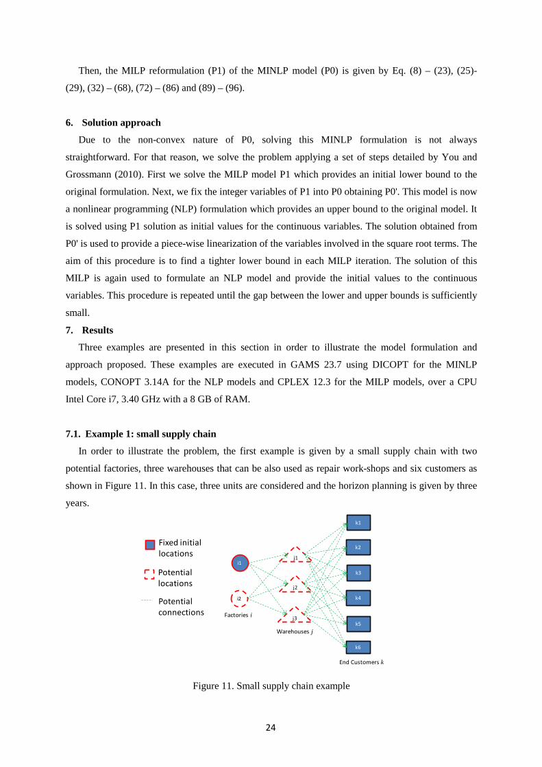
7.1. Example 1: small supply chain
In order to illustrate the problem, the first example is given by a small supply chain with two
potential factories, three warehouses that can be also used as repair work-shops and six customers as
shown in Figure 11. In this case, three units are considered and the horizon planning is given by three
years.
Figure 11. Small supply chain example
k5
i1
i2
j1
j2
j3
k1
k2
k3
k4
Fixed initial locations
Potential locations
k6
Potential connections Factories i
Warehouses j
End Customers k
25
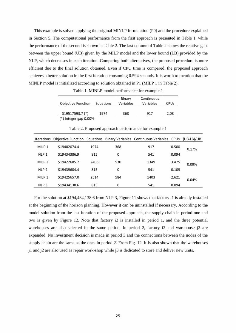
This example is solved applying the original MINLP formulation (P0) and the procedure explained
in Section 5. The computational performance from the first approach is presented in Table 1, while
the performance of the second is shown in Table 2. The last column of Table 2 shows the relative gap,
between the upper bound (UB) given by the MILP model and the lower bound (LB) provided by the
NLP, which decreases in each iteration. Comparing both alternatives, the proposed procedure is more
efficient due to the final solution obtained. Even if CPU time is compared, the proposed approach
achieves a better solution in the first iteration consuming 0.594 seconds. It is worth to mention that the
MINLP model is initialized according to solution obtained in P1 (MILP 1 in Table 2).
Table 1. MINLP model performance for example 1
Objective Function Equations Binary
Variables Continuous Variables CPUs
$19517593.7 (*) 1974 368 917 2.08 (*) Integer gap 0.00%
Table 2. Proposed approach performance for example 1
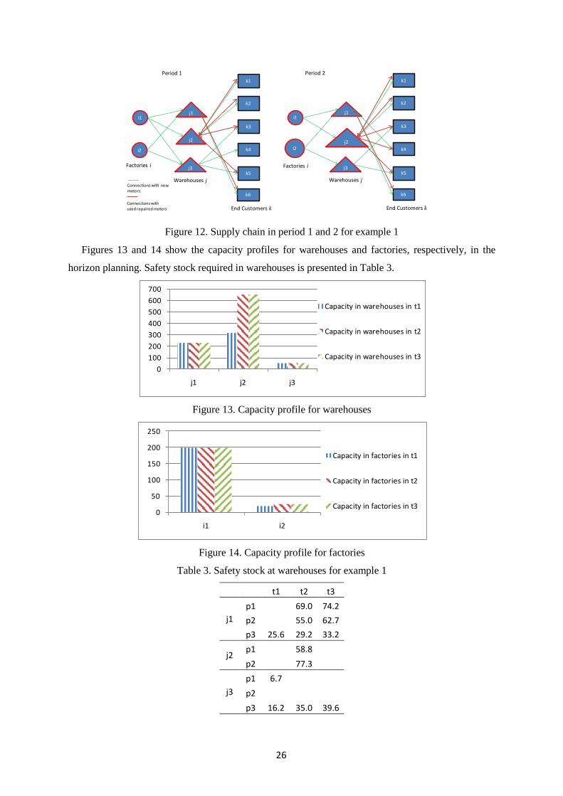
For the solution at $194,434,138.6 from NLP 3, Figure 11 shows that factory i1 is already installed
at the beginning of the horizon planning. However it can be uninstalled if necessary. According to the
model solution from the last iteration of the proposed approach, the supply chain in period one and
two is given by Figure 12. Note that factory i2 is installed in period 1, and the three potential
warehouses are also selected in the same period. In period 2, factory i2 and warehouse j2 are
expanded. No investment decision is made in period 3 and the connections between the nodes of the
supply chain are the same as the ones in period 2. From Fig. 12, it is also shown that the warehouses
j1 and j2 are also used as repair work-shop while j3 is dedicated to store and deliver new units.
Iterations Objective Function Equations Binary Variables Continuous Variables CPUs (UB-LB)/UB
MILP 1 $19402074.4 1974 368 917 0.500 0.17% NLP 1 $19434386.9 815 0 541 0.094
MILP 2 $19422685.7 2406 530 1349 3.475 0.09% NLP 2 $19439604.4 815 0 541 0.109
MILP 3 $19425657.0 2514 584 1403 2.621 0.04%
NLP 3 $19434138.6 815 0 541 0.094
26
Figure 12. Supply chain in period 1 and 2 for example 1
Figures 13 and 14 show the capacity profiles for warehouses and factories, respectively, in the
horizon planning. Safety stock required in warehouses is presented in Table 3.
Figure 13. Capacity profile for warehouses
Figure 14. Capacity profile for factories
Table 3. Safety stock at warehouses for example 1
t1 t2 t3
j1 p1 69.0 74.2 p2
55.0 62.7
p3 25.6 29.2 33.2
j2 p1 58.8 p2
77.3
j3 p1 6.7
p2 p3 16.2 35.0 39.6
k5
i1
i2
j1
j2
j3
k1
k2
k3
k4
k6
Factories i
Warehouses j
End Customers k
k5
i1
i2
j1
j2
j3
k1
k2
k3
k4
k6
Factories i
Warehouses j
End Customers k
Connections with new motors
Connections with used repaired motors
Period 1 Period 2
0100200300400500600700
j1 j2 j3
Capacity in warehouses in t1
Capacity in warehouses in t2
Capacity in warehouses in t3
0
50
100
150
200
250
i1 i2
Capacity in factories in t1
Capacity in factories in t2
Capacity in factories in t3
27
7.2. Example 2: Larger supply chain
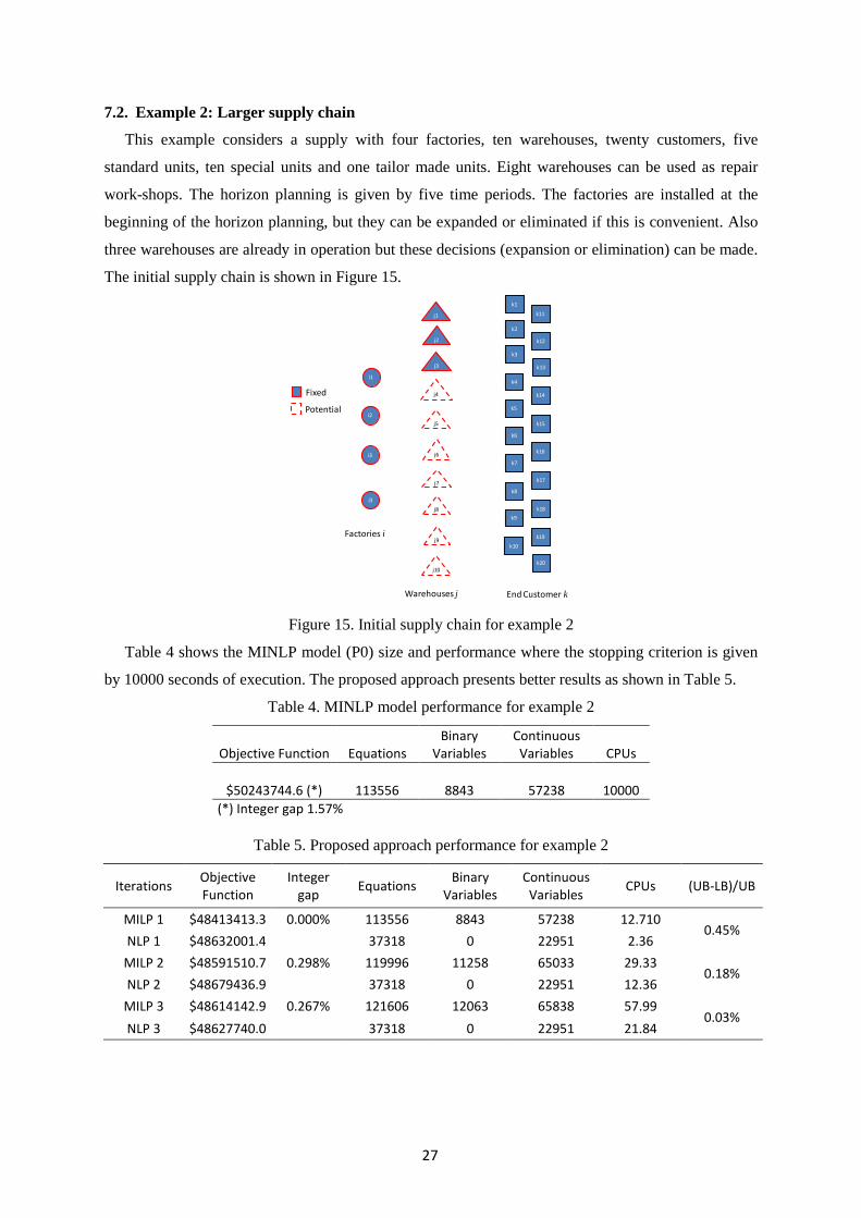
This example considers a supply with four factories, ten warehouses, twenty customers, five
standard units, ten special units and one tailor made units. Eight warehouses can be used as repair
work-shops. The horizon planning is given by five time periods. The factories are installed at the
beginning of the horizon planning, but they can be expanded or eliminated if this is convenient. Also
three warehouses are already in operation but these decisions (expansion or elimination) can be made.
The initial supply chain is shown in Figure 15.
Figure 15. Initial supply chain for example 2
Table 4 shows the MINLP model (P0) size and performance where the stopping criterion is given
by 10000 seconds of execution. The proposed approach presents better results as shown in Table 5.
Table 4. MINLP model performance for example 2
Objective Function Equations Binary
Variables Continuous Variables CPUs
$50243744.6 (*) 113556 8843 57238 10000 (*) Integer gap 1.57%
Table 5. Proposed approach performance for example 2
Iterations Objective Function
Integer gap Equations Binary
Variables Continuous Variables CPUs (UB-LB)/UB
MILP 1 $48413413.3 0.000% 113556 8843 57238 12.710 0.45%
NLP 1 $48632001.4 37318 0 22951 2.36 MILP 2 $48591510.7 0.298% 119996 11258 65033 29.33
0.18% NLP 2 $48679436.9 37318 0 22951 12.36
MILP 3 $48614142.9 0.267% 121606 12063 65838 57.99 0.03%
NLP 3 $48627740.0 37318 0 22951 21.84
k5
i1
i2
i3
j1
j2
j3
j4
k1
k2
k3
k4
Factories i
Warehouses j End Customer k
Fixed
Potential
i3
j5
j6
j7
j8
j9
j10
k10
k6
k7
k8
k9
k19
k11
k13
k15
k17
k20
k12
k14
k16
k18
28
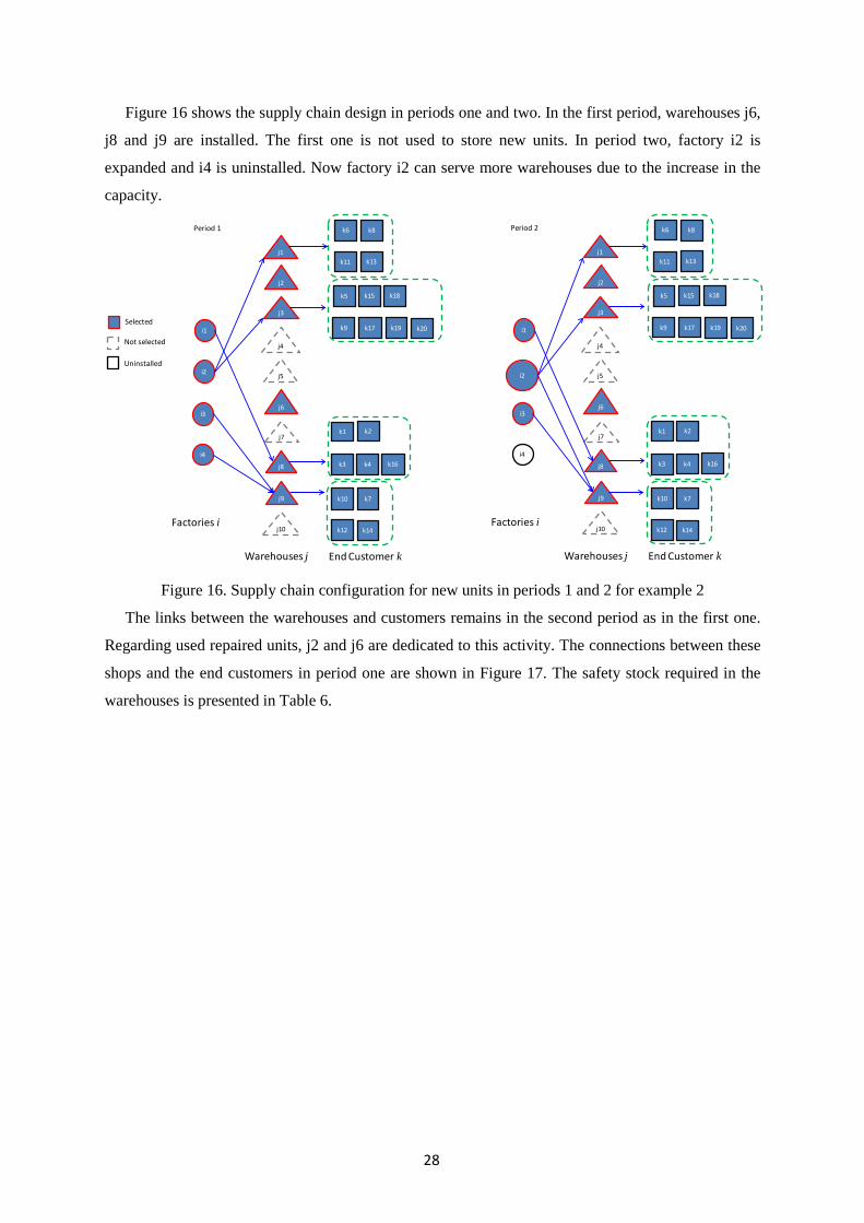
Figure 16 shows the supply chain design in periods one and two. In the first period, warehouses j6,
j8 and j9 are installed. The first one is not used to store new units. In period two, factory i2 is
expanded and i4 is uninstalled. Now factory i2 can serve more warehouses due to the increase in the
capacity.
Figure 16. Supply chain configuration for new units in periods 1 and 2 for example 2
The links between the warehouses and customers remains in the second period as in the first one.
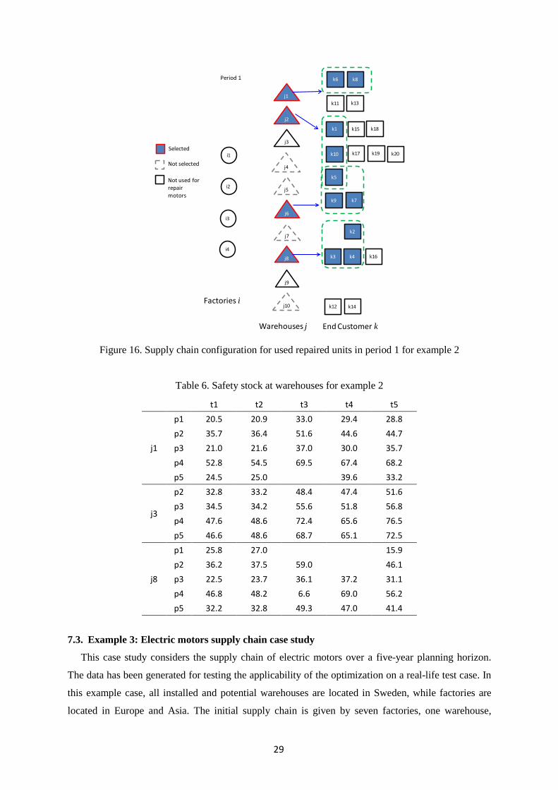
Regarding used repaired units, j2 and j6 are dedicated to this activity. The connections between these
shops and the end customers in period one are shown in Figure 17. The safety stock required in the
warehouses is presented in Table 6.
i1
i2
i3
j1
j2
j3
j4
k1 k2
Factories i
Warehouses j End Customer k
Selected
Not selected
i4
j5
j6
j7
j8
j9
j10
k10
k11
k15
k17 k20
k12 k14
k16k3
k18
k8
k19k9
k5
k4
k13
k7
k6Period 1
i1
i2
i3
j1
j2
j3
j4
k1 k2
Factories i
Warehouses j End Customer k
i4
j5
j6
j7
j8
j9
j10
k10
k11
k15
k17 k20
k12 k14
k16k3
k18
k8
k19k9
k5
k4
k13
k7
k6Period 2
Uninstalled
29
Figure 16. Supply chain configuration for used repaired units in period 1 for example 2
Table 6. Safety stock at warehouses for example 2
t1 t2 t3 t4 t5
j1
p1 20.5 20.9 33.0 29.4 28.8 p2 35.7 36.4 51.6 44.6 44.7 p3 21.0 21.6 37.0 30.0 35.7 p4 52.8 54.5 69.5 67.4 68.2 p5 24.5 25.0 39.6 33.2
j3
p2 32.8 33.2 48.4 47.4 51.6 p3 34.5 34.2 55.6 51.8 56.8 p4 47.6 48.6 72.4 65.6 76.5 p5 46.6 48.6 68.7 65.1 72.5
j8
p1 25.8 27.0 15.9 p2 36.2 37.5 59.0 46.1 p3 22.5 23.7 36.1 37.2 31.1 p4 46.8 48.2 6.6 69.0 56.2 p5 32.2 32.8 49.3 47.0 41.4
7.3. Example 3: Electric motors supply chain case study
This case study considers the supply chain of electric motors over a five-year planning horizon.
The data has been generated for testing the applicability of the optimization on a real-life test case. In
this example case, all installed and potential warehouses are located in Sweden, while factories are
located in Europe and Asia. The initial supply chain is given by seven factories, one warehouse,
i1
i2
i3
j1
j2
j3
j4
k1
k2
Factories i
Warehouses j End Customer k
Selected
Not selected
i4
j5
j6
j7
j8
j9
j10
k10
k11
k15
k17 k20
k12 k14
k16k3
k18
k8
k19
k9
k5
k4
k13
k7
k6Period 1
Not used for repair motors
30
which is not a repair workshop (j1) and 27 customers (k). No investments in new factories are allowed
and lost sales costs are disregarded. Four additional warehouses can be installed in any of the five
periods, and three of them can be repair workshops. A demand for 50 different motor types is
included in the model.
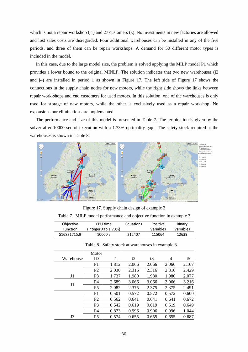
In this case, due to the large model size, the problem is solved applying the MILP model P1 which
provides a lower bound to the original MINLP. The solution indicates that two new warehouses (j3
and j4) are installed in period 1 as shown in Figure 17. The left side of Figure 17 shows the
connections in the supply chain nodes for new motors, while the right side shows the links between
repair work-shops and end customers for used motors. In this solution, one of the warehouses is only
used for storage of new motors, while the other is exclusively used as a repair workshop. No
expansions nor eliminations are implemented.
The performance and size of this model is presented in Table 7. The termination is given by the
solver after 10000 sec of execution with a 1.73% optimality gap. The safety stock required at the
warehouses is shown in Table 8.
Figure 17. Supply chain design of example 3
Table 7. MILP model performance and objective function in example 3
Table 8. Safety stock at warehouses in example 3
Warehouse Motor
ID t1 t2 t3 t4 t5
J1
P1 1.812 2.066 2.066 2.066 2.167 P2 2.030 2.316 2.316 2.316 2.429 P3 1.737 1.980 1.980 1.980 2.077
J1 P4 2.689 3.066 3.066 3.066 3.216 P5 2.082 2.375 2.375 2.375 2.491
J3
P1 0.501 0.572 0.572 0.572 0.600 P2 0.562 0.641 0.641 0.641 0.672 P3 0.542 0.619 0.619 0.619 0.649 P4 0.873 0.996 0.996 0.996 1.044 P5 0.574 0.655 0.655 0.655 0.687
Objective Function
CPU time (integer gap 1.73%)
Equations Positive Variables
Binary Variables
$16881715.9 10000 s 212407 115064 12639

31
8. Conclusions
We have developed an MINLP model to determine the optimal supply chain structure over a multi-
period horizon planning considering demand uncertainty. Network decisions include the selection of
new locations and the links that connect the different nodes in the supply chain in each period. Special
characteristics from the electric motors industry are considered such as the demand of failing units
that are at customer plants, and how this demand can be satisfied with new or used spare parts by the
company. However, this model is generic and can also be applied to other type of industries. Model
decisions such as new investment, capacity expansion and elimination of assets allow not only the
design, but also the evaluation and re-design of a supply chain that is already in operation. From the
inventory management perspective, safety stock, mean stock levels, capacity constraints and lost sales
costs are also taken into account to satisfy customer orders according to the company commitments.
Part II of this paper presents a decomposition approach in order to solve larger instances as well as to
obtain a lower gap in reasonable computational time.
Acknowledgments
The authors gratefully acknowledge financial support for ABB through the Center for Advanced
Process Decision-making, CONICET and Universidad Tecnologica Nacional.
Nomenclature
Sets
c Criticality levels of motors i Factories j Warehouses k End customers p Standard units s Special units t Time periods
ksCT Customers k that allow used repaired units to satisfy their demand of units JF Subset of warehouses j that are already installed (fixed) at the beginning of the horizon planning
kscKSC Customers k that order special units s of criticality c
ksKT Customers k that order tailor made units s psPS Special units s belonging to standard unit p
SC Subset of warehouses j that can be also considered as repair workshops
Binary variables
ikstu if factory i produces and delivers tailor made unit s to end customer k in period t
32
jkstv if repair workshop j repairs special units s from customer k in period t
itw if factory i is installed in period t e
itw if warehouse j is expanded in period t uitw if factory i is uninstalled (eliminated) in period t
ijptx if factory i produces and delivers standard units p to warehouse j in period t
jty if warehouse j is installed in period t ejty if warehouse j is expanded in period t ujty if warehouse j is uninstalled (eliminated) in period t
jktz if warehouse j delivers units to customer k in period t Positive variables
jtce capacity expansion of warehouse j in period t 𝑐𝑒𝑓𝑖𝑡capacity expansion of factory i in period t
ksctl net lead time of customer k for special unit s of criticality c in period t
' jksctl net lead time of customer k if special unit s of criticality c is provided by warehouse j in period t
ksctm net lead time of customer k for tailor made unit s of criticality c in period t
'iksctm net lead time of customer k if tailor made unit s of criticality c is provided by warehouse j in period t
jptn net lead time of warehouse j for standard unit p in period t
jtq capacity of warehouse j in period t 𝑞𝑓𝑖𝑡capacity of factory i in period t
jpts guaranteed service time of warehouse j to its successive nodes in the supply chain for standard unit p in period t
jptss safety stock of warehouse j for standard unit p in period t
jtuc capacity eliminated from warehouse j in period t (when the warehouse is uninstalled) 𝑢𝑐𝑓𝑖𝑡capacity eliminated from factory i in period t (when the factory is uninstalled)
newijkptµ amount of demand of standard units p from customer k satisfied with new units from factory
i and warehouse j usedjkstµ amount of demand of special units s from customer k satisfied with used units from repair
workshop j newikstτ amount of demand of tailor made units p from customer k satisfied with new units from
factory i usedjkstτ amount of demand of tailor made units s from customer k satisfied with used units from
repair workshop j
Parameters
1ksb unit annual lost sales cost for special unit s at customer k
1ijc unit transportation cost from factory i to warehouse j
33
2 jkc unit transportation cost from warehouse j to customer k
3ikc unit transportation cost from factory i to customer k
ksd Fraction of demand that is back ordered or lost (customer disservice) for special unit s from
end customer k jec expansion investment cost for warehouse j
𝑒𝑐𝑝𝑖expansion investment cost for factory i
jf investment cost for installing warehouse j
𝑓𝑝𝑖 investment cost for installing factory i
jg variable handling cost of warehouse j
isGI guaranteed service time of factory i for tailor made unit s
igp variable production cost of factory i
jpgr variable repairing cost of repair workshop j for standard unit p ' jsgr variable repairing cost of repair workshop j for tailor made unit s
1 jph unit safety stock cost for standard unit p in warehouse j
2kh unit safety stock cost at customer k
jIC initial capacity of warehouse j 𝐼𝐶𝐹𝑖initial capacity of factory i
ir interest rate
jofc operational fixed cost for warehouse j
𝑝𝑓𝑐𝑖operational fixed cost for factory i
ksQ Reorder quantity for special unit s from end customer k UPjQDC maximal capacity expansion in each period for warehouse j
UPiQP capacity of factory i
kscR guaranteed service time expected by customer k for special unit s of criticality c
ksrp repairing probability of special unit s from customer k
ipSI guaranteed service time of factory i for standard unit p
1ijpt order processing time of warehouse j for standard unit p if it is served by plant i, including material handling time in j, transportation time from plant i to j, and inventory review period in the warehouse 2 jkpt order processing time of customer k for standard unit p if it is served by warehouse j,
including material handling time in k, transportation time from warehouse j to k, and inventory review period in the customer site 3ikst order processing time of customer k for tailor made unit s if it is served by plant i, including
material handling time in k, transportation time from plant i to k, and inventory review period in the customer site
34
jptsu average time that used standard units p are kept in storage in warehouse j
jsttu average time that used tailor made units s are kept in storage in warehouse j
juc investment cost if warehouse j is uninstalled 𝑢𝑐𝑝𝑖investment cost if factory i is uninstalled
pα production factor rate for standard unit p
pβ size factor for standard unit p
2sβ size factory for special unit s
jpλ safety factor of warehouse j for standard unit p
2ksλ safety factor of customer k for special unit s
ksctµ mean demand of special units s of criticality c from customer k in period t 1 jpθ unit inventory cost for standard unit p in warehouse j
2kpθ unit inventory cost for standard unit p in customer k
ksctσ demand standard deviation of special units s of criticality c from customer k in period t χ days in the year
References Bossert, J.M. and Willems, S.P. A periodic-review modeling approach for guaranteed service supply chains.
Interfaces. 2007, 37, 5, 420–435.
Charnes, A. and Cooper, W.W. Deterministic equivalents for optimizing and satisfying under chance
constraints. Operations Research. 1963, 11, 18–39.
Daskin, M.S., Coullard, C.R. and Shen, Z.J.M. An Inventory-Location Model: Formulation, Solution
Algorithm and Computational Results. Annals of Operations Research 110, 83–106, 2002.Kluwer Academic
Publishers. The Netherlands.
Eppen, G.D. Effect of centralization on expected costs in a multi-location newsboy problem. Management
Science, 1979, 25, 5, 498–501.
Grossmann, I.E. Enterprise-wide Optimization: A New Frontier in Process Systems Engineering. AIChE
Journal, 2005, 51, 7, 1846–1857.
Gupta, A. and Maranas, C.D. Managing demand uncertainty in supply chain planning. Computers and
Chemical Engineering. 2003, 27, 1219–1227.
Little, J.D.C. A proof of the queueing formula L=λW. Operation Research. 1961, 9, 383–387.
Nyberg, A., Grossmann, I.E. and Westerlund, T. An Efficient Reformulation of the Multiechelon Stochastic
Inventory System with Uncertain Demands. AIChE Journal. 2013, 59, 23–28.
Parker, L.L. Economical reorder quantities and reorder points with uncertain demand. Naval Research
Logistics Quarterly. 1964, 11, 4, 351–358.
Rodriguez, M.A., Vecchietti, A. Multicriteria optimization model for supply process problem under
provision and demand uncertainty. Industrial and Engineering Chemistry Research. 2011, 50, 10630–10642.
35
Sahinidis, N.V. Optimization under uncertainty: state-of-the-art and opportunities. Computers and Chemical
Engineering. 2004, 28, 971–983.
Santoso, T., Ahmed, S., Goetschalckx, M. and Shapiro A. A stochastic programming approach for supply
chain network design under uncertainty. European Journal of Operational Research. 2005, 167, 96–115.
Shen, S.J.M., Coullard, C. and Daskin, M.S. A Joint Location-Inventory Model. Transportation Science.
2003, 37, 1, 40–55.
You, F. and Grossmann, I.E. Design of responsive supply chains under demand uncertainty. Computers and
Chemical Engineering. 2008, 32, 3090–3111.
You, F. and Grossmann, I.E. Integrated Multi-Echelon Supply Chain Design with Inventories Under
Uncertainty: MINLP Models, Computational Strategies. AIChE Journal, 2010, 56, 2, 419–440.
Zipkin, P.H. Foundations of Inventory Management. Boston, MA. McGraw-Hill, 2000.
Recommended