109 ' # '7& *#1 & 8 - Opencdn.intechopen.com/pdfs-wm/15529.pdf · Supply Chain Optimization: Centralized vs Decentralized Planning ... Optimal control policies are ... Supply Chain

3,350+OPEN ACCESS BOOKS

108,000+INTERNATIONAL

AUTHORS AND EDITORS114+ MILLION

DOWNLOADS

BOOKSDELIVERED TO

151 COUNTRIES

AUTHORS AMONG

TOP 1%MOST CITED SCIENTIST

12.2%AUTHORS AND EDITORS

FROM TOP 500 UNIVERSITIES

Selection of our books indexed in theBook Citation Index in Web of Science™

Core Collection (BKCI)

Chapter from the book Supply Chain ManagementDownloaded from: http://www.intechopen.com/books/supply-chain-management

PUBLISHED BY

World's largest Science,Technology & Medicine

Open Access book publisher

Interested in publishing with IntechOpen?Contact us at [email protected]

http://www.intechopen.com/books/supply-chain-management

mailto:[email protected]

1

Supply Chain Optimization: Centralized vs Decentralized Planning and Scheduling

Georgios K.D. Saharidis 1University of Thessaly, Department of Mechanical Engineering

2Kathikas Institute of Research and Technology 1Greece

2USA

1. Introduction

In supply chain management manufacturing flow lines consist of two or more work areas, arranged in series and/or in parallel, with intermediate storage areas. The first work area processes raw items and the last work area produces end items or products, which are stored in a storage area in anticipation of future demand. Firstly managers should analyze and organize the long term production optimizing the production planning of the supply chain. Secondly, they have to optimize the short term production analyzing and organizing the production scheduling of the supply chain and finally taking under consideration the stochasticity of the real world, managers have to analyze and organize the performance of the supply chain adopting the best control policy. In supply chain management production planning is the process of determining a tentative plan for how much production will occur in the next several time periods, during an interval of time called the planning horizon. Production planning also determines expected inventory levels, as well as the workforce and other resources necessary to implement the production plans. Production planning is done using an aggregate view of the production facility, the demand for products and even of time (ex. using monthly time periods). Production planning is commonly defined as the cross-functional process of devising an aggregate production plan for groups of products over a month or quarter, based on management targets for production, sales and inventory levels. This plan should meet operating requirements for fulfilling basic business profitability and market goals and provide the overall desired framework in developing the master production schedule and in evaluating capacity and resource requirements. In supply chain management production scheduling defines which products should be produced and which products should be consumed in each time instant over a given small time horizon; hence, it defines which run-mode to use and when to perform changeovers in order to meet the market needs and satisfy the demand. Large-scale scheduling problems arise frequently in supply chain management where the main objective is to assign sequence of tasks to processing units within certain time frame such that demand of each product is satisfied before its due date. For supply chain systems the aim of control is to optimize some performance measure, which typically comprises revenue from sales less the costs of inventory and those

www.intechopen.com

Supply Chain Management

4

associated with the delays in filling customer orders. Control is dynamic and affects the rate of accepted orders and the production rates of each work area according to the state of the system. Optimal control policies are often of the bang-bang type, that is, they determine when to start and when to stop production at each work area and whether to accept or deny an incoming order. A number of flow control policies have been developed in recent years (see, e.g., Liberopoulos and Dallery 2000, 2003). Flow control is a difficult problem, especially in flow lines of the supply chain type, in which the various work and storage areas belong to different companies. The problem becomes more difficult when it is possible for companies owning certain stages of the supply chain to purchase a number of items from subcontractors rather than producing these items in their plants. In general, a good planning, scheduling and control policy must be beneficial for the whole supply chain and for each participating company. In practice, however, each company tends to optimize its own production unit subject to certain constraints (e.g., contractual obligations) with little attention to the remaining stages of the supply chain. For example, if a factory of a supply chain purchases raw items regularly from another supply chain participant, then, during stockout periods, the company which owns that factory may occasionally find it more profitable to purchase a quantity immediately from some subcontractor outside the supply chain, rather than wait for the delivery of the same quantity from its regular supplier. Although similar policies (decentralized policies) can be individually optimal at each stage of the supply chain, the sum of the profits collected individually can be much lower than the maximum profit the system could make under a coordinated policy (centralized policies). The rest of this paper is organized as follows. Section 2 a literature review is presented. In section 3, 4 and 5 three cases studies are presented where centralized and decentralized optimization is applied and qualitative results are given. Section 5 draws conclusions.

2. Literature review

There are relatively few papers that have addressed planning and scheduling problems using centralized and decentralized optimization strategies providing a comparison of these two approaches. (Bassett et al., 1996) presented resource decomposition method to reduce problem complexity by dividing the scheduling problem into subsections based on its process recipes. They showed that the overall solution time using resource decomposition is significantly lower than the time needed to solve the global problem. However, their proposed resource decomposition method did not involve any feedback mechanism to incorporate “raw material” availability between sub sections. (Harjunkoski and Grossmann, 2001) presented a decomposition scheme for solving large scheduling problems for steel production which splits the original problem into sub-systems using the special features of steel making. Numerical results have shown that the proposed approach can be successfully applied to industrial scale problems. While global optimality cannot be guaranteed, comparison with theoretical estimates indicates that the method produces solutions within 1–3% of the global optimum. Finally, it should be noted that the general structure of the proposed approach naturally would allow the consideration of other types of problems, especially such, where the physical problem provides a basis for decomposition. (Gnoni et al., 2003) present a case study from the automotive industry dealing with the lot sizing and scheduling decisions in a multi-site manufacturing system with uncertain multi-

www.intechopen.com


5

product and multi-period demand. They use a hybrid approach which combines mixed-integer linear programming model and simulation to test local and global production strategies. The paper investigates the effects of demand variability on the economic performance of the whole production system, using both local and global optimization strategies. Two different situations are compared: the first one (decentralized) considers each manufacturing site as a stand-alone business unit using a local optimization strategy; the second one (centralized) considers the pool of sites as a single manufacturing system operating under a global optimization strategy. In the latter case, the problem is solved by jointly considering lot sizes and sequences of all sites in the supply chain. Results obtained are compared with simulations of an actual reference annual production plan. The local optimization strategy allows a cost reduction of about 19% compared to the reference actual situation. The global strategy leads to a further cost reduction of 3.5%, smaller variations of the cost around its mean value, and, in general, a better overall economic performance, although it causes local economic penalties at some sites. (Chen and Chen, 2005) study a two-echelon supply chain, in which a retailer maintains a stock of different products in order to meet deterministic demand and replenishes the stock by placing orders at a manufacturer who has a single production facility. The retailer’s problem is to decide when and how much to order for each product and the manufacturer’s problem is to schedule the production of each product. The authors examine centralized and decentralized control policies minimizing respectively total and individual operating costs, which include inventory holding, transportation, order processing, and production setup costs. The optimal decentralized policy is obtained by maximizing the retailer’s cost per unit time independently of the manufacturer’s cost. On the contrary, the centralized policy minimizes the total cost of the system. An algorithm is developed which determines the optimal order quantity and production cycle for each product. It should be noted that the same model is applicable to multi-echelon distribution/inventory systems in which a manufacturer supplies a single product to several retailers. Several numerical experiments demonstrate the performance of the proposed models. The numerical results show that the centralized policy significantly outperforms the decentralized policy. Finally, the authors present a savings sharing mechanism whereby the manufacturer provides the retailer with a quantity discount which achieves a Pareto improvement among both participants of the supply chain. (Kelly and Zyngier, 2008) presented a new technique for decomposing and rationalizing large decision-making problems into a common and consistent framework. The focus of this paper has been to present a heuristic, called the hierarchical decomposition heuristic (HDH), which can be used to find globally feasible solutions to usually large decentralized and distributed decision-making problems when a centralized approach is not possible. The HDH is primarily intended to be applied as a standalone tool for managing a decentralized and distributed system when only globally consistent solutions are necessary or as a lower bound to a maximization problem within a global optimization strategy such as Lagrangean decomposition. The HDH was applied to an illustrative example based on an actual industrial multi-site system as well as to three small motivating examples and was able to solve these problems faster than a centralized model of the same problems when using both coordinated and collaborative approaches. (Rupp et al., 2000) present a fine planning for supply chains in semiconductor manufacturing. It is generally accepted that production planning and control, in the make-to-order environment of application-specific integrated circuit production, is a difficult task,

www.intechopen.com


6

as it has to be optimal both for the local manufacturing units and for the whole supply chain network. Centralised MRP II systems which are in operation in most of today’s manufacturing enterprises are not flexible enough to satisfy the demands of this highly dynamic co-operative environment. In this paper Rupp et al. present a distributed planning methodology for semiconductor manufacturing supply chains. The developed system is based on an approach that leaves as much responsibility and expertise for optimisation as possible to the local planning systems while a global co-ordinating entity ensures best performance and efficiency of the whole supply chain.

3. Centralized vs decentralized deterministic planning: A case study of seasonal demand of aluminium doors

3.1 Problem description

In this section, we study the production planning problem in supply chain involving several

enterprises whose final products are doors and windows made out of aluminum and

compare two approaches to decision-making: decentralized versus centralized. The first

enterprise is in charge of purchasing the raw materials and producing a partially competed

product, whereas the second enterprise is in charge of designing the final form of the

product which needs several adjustments before being released to the market. Some of those

adjustments is the placement of several small parts, the addition of paint and the placement

of glass pieces.

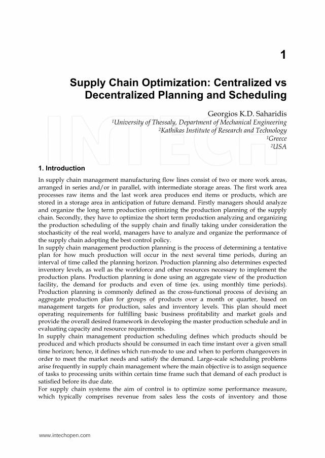
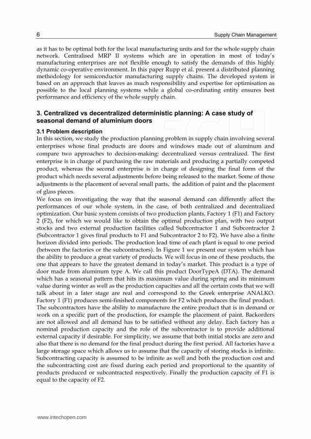
We focus on investigating the way that the seasonal demand can differently affect the performances of our whole system, in the case, of both centralized and decentralized optimization. Our basic system consists of two production plants, Factory 1 (F1) and Factory 2 (F2), for which we would like to obtain the optimal production plan, with two output stocks and two external production facilities called Subcontractor 1 and Subcontractor 2 (Subcontractor 1 gives final products to F1 and Subcontractor 2 to F2). We have also a finite horizon divided into periods. The production lead time of each plant is equal to one period (between the factories or the subcontractors). In Figure 1 we present our system which has the ability to produce a great variety of products. We will focus in one of these products, the one that appears to have the greatest demand in today’s market. This product is a type of door made from aluminum type A. We call this product DoorTypeA (DTA). The demand which has a seasonal pattern that hits its maximum value during spring and its minimum value during winter as well as the production capacities and all the certain costs that we will talk about in a later stage are real and correspond to the Greek enterprise ANALKO. Factory 1 (F1) produces semi-finished components for F2 which produces the final product. The subcontractors have the ability to manufacture the entire product that is in demand or work on a specific part of the production, for example the placement of paint. Backorders are not allowed and all demand has to be satisfied without any delay. Each factory has a nominal production capacity and the role of the subcontractor is to provide additional external capacity if desirable. For simplicity, we assume that both initial stocks are zero and also that there is no demand for the final product during the first period. All factories have a large storage space which allows us to assume that the capacity of storing stocks is infinite. Subcontracting capacity is assumed to be infinite as well and both the production cost and the subcontracting cost are fixed during each period and proportional to the quantity of products produced or subcontracted respectively. Finally the production capacity of F1 is equal to the capacity of F2.

www.intechopen.com


7

Fig. 1. The two-stage supply chain of ANALKO

On the one hand in the decentralized approach, we have two integrated local optimization problems from the end to the beginning. Namely, we first optimize the production plan of F2 and then that of F1. On the other hand, in centralized optimization we take into account all the characteristics of the production in the F1 and F2 simultaneously and then we optimize our system globally. The initial question is: What is to be gained by centralized optimization in contrast to decentralized?

3.2 Methodology

Two linear programming formulations are used to solve the above problems. In appendix A all decision variables and all parameters are presented:

3.2.1 Centralized optimization

The developed model, taking under consideration the final demand and the production capacity of two factories as well as the subcontracting and inventories costs, optimizes the overall operation of the supply chain. The objective function has the following form:

2

, , ,1 1 1 1

Z [ csc ]T T T

i i t i i t i i ti t t t

Min cp P h I SC= = = =

= + +∑ ∑ ∑ ∑ (1)

The constraints of the problem are mainly two: a) the material balance equations:

1, 1, 1 1, 1, 2, 2,t t t t t tI I P SC P SC−= + + − − , t∀ (2)

2, 2, 1 2, 2,t t t t tI I P SC d−= + + − , t∀ (3)

1, 2, 0t TI I= = (4)

and b) the capacity of production:

Pi,t ≤ production capacity of factory i during period t (5)

1, 2,1 0TP P= = (6)

3.2.2 Decentralized optimization

In decentralized optimization two linear mathematical models are developed. The fist one optimizes the production of Factory 2 satisfying the total demand in each period under the capacity and material balance constraints of its level:

www.intechopen.com


8

2 2, 2 2, 2 2,1 1 1

Z cscT T T

t t tt t t

Min cp P h I SC= = =

= + +∑ ∑ ∑ (7)

subject to balance equations:

2, 2, 1 2, 2,t t t t tI I P SC d−= + + − , t∀ (8)

2, 0TI = (9)

and production capacity:

P2,t ≤ production capacity of factory 2 during period t , t∀ (10)

2,1 0P = (11)

The second model optimizes the production of Factory 1 satisfying the total demand coming from Factory 2 in each period under the capacity and material balance constraints of its level:

1 1, 1 1, 1 1,1 1 1

Z cscT T T

t t tt t t


= + +∑ ∑ ∑ (12)

subject to balance equations:

1, 1, 1 1, 1, 2, 2,t t t t t tI I P SC P SC−= + + − − , t∀ (13)

1, 0tI = (14)

and production capacity:

P2,t ≤ production capacity of factory 2 during period t , t∀ (15)

1, 0TP = (16)

3.3 Qualitative results We have used these two models to explore certain qualitative behavior of our supply chain. First of all we proved that the system’s cost of centralized optimization is less than or equal to that of decentralized optimization (property 1). Proof: This property is valid because the solution of decentralized optimization is a feasible solution for the centralized optimization but not necessarily the optimal solution ■ In terms of each one factory’s costs, the F2’s production cost in local optimization is less than or equal to that of global (property 2). Proof: The solution of decentralized optimization is a feasible solution for the centralized optimization but not necessarily the optimal centralized solution ■ In terms of F1’s optimal solution and using property 1 and 2 it is proved that the production cost in decentralized optimization is greater than or equal to that of centralized optimization (property 3). In reality for the subcontractor the cost of production cost for one unit is about the same as that of an affiliate company. The subcontractor in accordance with the contract rules wishes

www.intechopen.com


9

to receive a set amount of earnings that will not fluctuate and will be independent of the market tendencies. Thus when the market needs change, the production cost and the subcontracting cost change but the fixed amount of earnings mentioned in the contract stays the same. The system’s optimal production plan is the same when the difference between the production cost and the subcontracting cost stays constant as well as the difference between the costs of local and global optimization is constant (property 4). Using this property we are not obliged to change the production plan when the production cost changes. In addition, in some cases, we could be able to avoid one of two analyses.

Proof: If for factory F2, 2 2 2 2 2csc csccp cp′ ′Δ = − = − where 2 2csc csc′≠ and 2 2cp cp′≠ then it is enough to demonstrate that the optimal value of the objective function as well as the optimal production plan are the same when the production cost and the subcontracting cost are 2 2,csccp and when the production cost and the subcontracting cost are 2 2,csccp′ ′ . For

2 2, csccp′ ′ , we take the following objective function:

2 2, 2 2, 2 2,1 1 1

Z cscT T T

t t tt t t


′ ′= + +∑ ∑ ∑ (17)

Subject to: Balance equations:

2, 2, 1 2, 2,t t t t tI I P SC d−= + + − , t∀ (18)

2, 0TI = (19)

Production capacity:

P2,t ≤ production capacity of factory 2 during period t, t∀ (20)

2,1 0P = (21)

It is also valid that:

2, 2,1 1

T T

t t tt t

P SC d= =

+ =∑ ∑ , t∀ (22)

2 2 2csc cp′ ′− = Δ (23)

Using equalities (22), (23) the objective function becomes:

2 2, 2 2, 2 2,1 1 1

Z [ ] cscT T T

t t t tt t t

Min cp d SC h I SC= = =

′ ′= − + + ⇒∑ ∑ ∑

2 2 2, 2 2 2, 2 21 1 1

Z (csc ) (csc )T T T

t t tt t t

Min cp d h I cp SC cp= = =

′ ′ ′ ′ ′= + + − ⇒ − = Δ∑ ∑ ∑

2 2 2, 2 2,1 1 1

Z T T T

t t tt t t

Min cp d h I SC= = =

′= + + Δ∑ ∑ ∑ (24)

www.intechopen.com


10

Following the same procedure and using as production cost and subcontracting cost 2csc ,

2cp the objective function becomes:

2 2 2, 2 2,

1 1 1

Z T T T

t t tt t t

Min cp d h I SC= = =

= + + Δ∑ ∑ ∑ (25)

Objective function (24) and (25) have the same components (except the constant term

21

T

tt

cp d=∑ which does not influence the optimization). This results the same minimum value

and exactly the same production plan due to the same group of constraints (13)-(14)■ When the centralized optimization gives an optimal solution for F2 to subcontract the extra demand regardless of F1’s plan, the decentralized optimization gives exactly the same solution (property 5). Proof: In this case F1 obtains the demand curve which is exactly the same to the curve of the final product. In the case of decentralized optimization (which gives the optimal solution for F2) in the worst scenario we will get a production plan which follow the demand or a mix plan (subcontracting and inventory). The satisfaction of the first curve (centralized optimization) is more expensive for F1 than the satisfaction of the second (decentralized optimization) because the supplementary (to the production capacity) demand is greater. For this reason the production cost of F1 in decentralized optimization is greater than or equal to the production cost of the centralized optimization and using property 2 we prove that centralized and decentralized optimal production cost for F1 should be the same ■ Finally, we have demonstrated that when at the decentralized optimization, the extra demand for F2 is satisfied from inventory then the centralized optimization has the same optimal plan (property 6). Proof: In this case of decentralized optimization, F1 has the best possible curve of demand because F2 satisfy the extra demand without subcontracting. In centralized optimization in the best scenario we take the same optimal solution for F2 or a mix policy. If we take the case of mix policy then the centralized optimal solution of F1 will be greater than or equal to the decentralized optimal solution and using property 3 we prove that centralized and decentralized optimal production cost for F1 should be the same■

4. Centralized vs decentralized deterministic scheduling: A case study from petrochemical industry

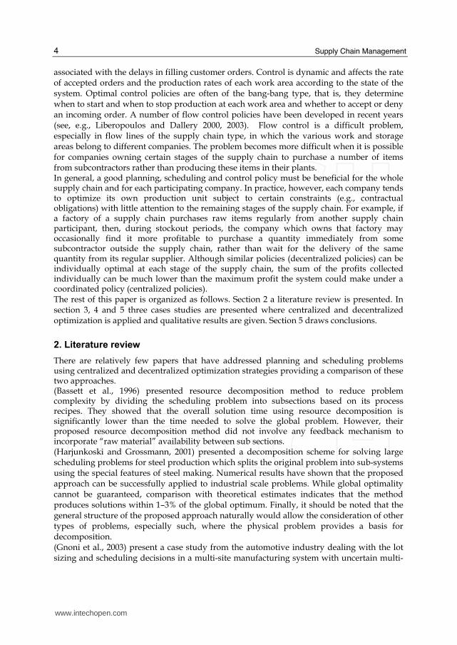
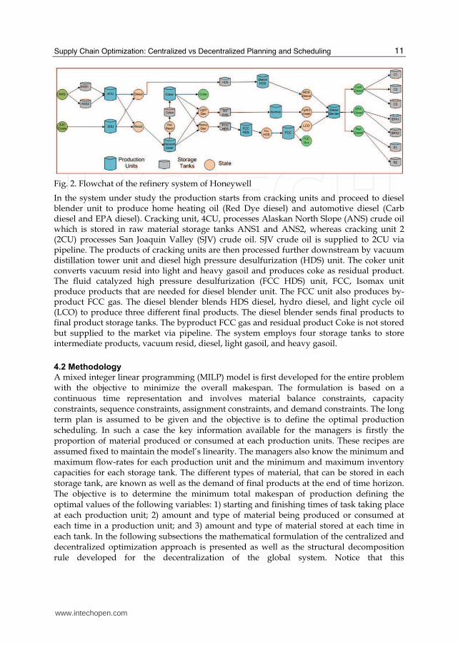
4.1 Problem description Refinery system considered here is composed of pipelines, a series of tanks to store the crude oil (and prepare the different mixtures), production units and tanks to store the raw materials and the intermediate and final products (see Figure 2). All the crude distillation units are considered continuous processes and it is assumed that unlimited supply of the raw material is available to system. The crude distillation unit produces different products according to the recipes. The production flow of our refinery system provided by Honeywell involves 9 units as shown in Figure 2. It starts from crude distillation units that consume raw materials ANS and SJV crude, to diesel blender that produces CARB diesel, EPA diesel and red dye diesel. The other two final products are coker and FCC gas. All the reactions are considered as continuous processes. We consider the operating rule for the storage tanks where material cannot flow out of the tank when material is flowing into the tank at any time interval, that is loading and unloading cannot happen simultaneously. This rule is imposed in many petrochemical companies for security and operating reasons.

www.intechopen.com


11

Fig. 2. Flowchat of the refinery system of Honeywell

In the system under study the production starts from cracking units and proceed to diesel blender unit to produce home heating oil (Red Dye diesel) and automotive diesel (Carb diesel and EPA diesel). Cracking unit, 4CU, processes Alaskan North Slope (ANS) crude oil which is stored in raw material storage tanks ANS1 and ANS2, whereas cracking unit 2 (2CU) processes San Joaquin Valley (SJV) crude oil. SJV crude oil is supplied to 2CU via pipeline. The products of cracking units are then processed further downstream by vacuum distillation tower unit and diesel high pressure desulfurization (HDS) unit. The coker unit converts vacuum resid into light and heavy gasoil and produces coke as residual product. The fluid catalyzed high pressure desulfurization (FCC HDS) unit, FCC, Isomax unit produce products that are needed for diesel blender unit. The FCC unit also produces byproduct FCC gas. The diesel blender blends HDS diesel, hydro diesel, and light cycle oil (LCO) to produce three different final products. The diesel blender sends final products to final product storage tanks. The byproduct FCC gas and residual product Coke is not stored but supplied to the market via pipeline. The system employs four storage tanks to store intermediate products, vacuum resid, diesel, light gasoil, and heavy gasoil.

4.2 Methodology

A mixed integer linear programming (MILP) model is first developed for the entire problem with the objective to minimize the overall makespan. The formulation is based on a continuous time representation and involves material balance constraints, capacity constraints, sequence constraints, assignment constraints, and demand constraints. The long term plan is assumed to be given and the objective is to define the optimal production scheduling. In such a case the key information available for the managers is firstly the proportion of material produced or consumed at each production units. These recipes are assumed fixed to maintain the model’s linearity. The managers also know the minimum and maximum flow-rates for each production unit and the minimum and maximum inventory capacities for each storage tank. The different types of material, that can be stored in each storage tank, are known as well as the demand of final products at the end of time horizon. The objective is to determine the minimum total makespan of production defining the optimal values of the following variables: 1) starting and finishing times of task taking place at each production unit; 2) amount and type of material being produced or consumed at each time in a production unit; and 3) amount and type of material stored at each time in each tank. In the following subsections the mathematical formulation of the centralized and decentralized optimization approach is presented as well as the structural decomposition rule developed for the decentralization of the global system. Notice that this

www.intechopen.com


12

decentralization rule is generally applicable in this type of system where intermediate stock areas (eg. tanks) appear and in the same time the production is a continuous process. In the end of this section an analytical mathematical proof is given in order to demonstrate that the application of this structural decomposition rule, for the decentralization of the system, gives the same optimal solution as the centralize optimization.

4.2.1 Centralized optimization

In this section the centralized mathematical model is presented. Notice that all parameters of the problem as well as the decision variables are given in appendix B. The objective function of the problem is the minimization of makespan (H). The most common motivation for optimizing the process using minimization of makespan as objective function is to improve customer services by accurately predicting order delivery dates.

min H (26)

Constraints (27) to (29) define binary variables wv, in, and out, which are 1 when reaction, input flow transfer to tanks and output flow transfer from tanks occur at event point n,

respectively. Otherwise, they become 0. Variable ( , , )in j jst n is equal to 1 if there is flow of

material from production unit (j) to storage tank (jst) at event point (n); otherwise it is equal to

0. Variable ( , , )out jst j n is equal to 1 if material is flowing from storage (jst) to unit (j) at

event point (n), otherwise it is equal to 0. Equations (28) and (29) are capacity constraints for storage tank. Constraints (28) state that if there is material inflow to tank (jst) at interval (n) then total amount of material inflow to the tank should not exceed the maximum storage capacity limit. Similarly, constraints (29) state that if there is outflow from tank (jst) at interval (n) then the total amount of material flowing out of tank should not exceed the storage limit at event point (n).

, , , ,*i j n i j nb U wv≤ (27)

max, , , ,inflow *j jst n jst j jst nV in≤ (28)

max, , , ,outflow *j jst n jst j jst nV out≤ (29)

Material balance constrains (30) state that the inventory of a storage tank at one event point

is equal to that at previous event point adjusted by the input and output stream amount.

, , 1 , , , , ,inflow inflow1jst jst

jst n jst n j jst n jst n j jst nj Jprodst j Jstprod

St St outflow− ∈ ∈= + + −∑ ∑ (30)

The production of a reactor (31) should be equal to the sum of amount of flows entering its

subsequent storage tanks and reactors, and the delivery to the market.

, , , , , , , ','

inflow unitflowJ j S j s

Ps i i j n j jst n s j j n

i I jst JSTprodst JST j Jseq Junitc

bρ∈ ∈ ∈

= +∑ ∑ ∑∩ ∩

, ,outflow2s j n+ (31)

Similarly, the consumption of a reactor (32) is equal to the sum of amount of streams coming

from preceding storage tanks and previous reactors, and stream coming from supply.

www.intechopen.com


13

, , , , ,*J j S

Cs i i j n jst j n

i I jst Jstprod JST

b outflowρ∈ ∈

= +∑ ∑∩

, , ', , ,'

inf 2j s

s j j n s j nj Jseq Junitp

unitflow low∈

+∑∩

(32)

Demand for each final product rs must be satisfied in centralized problem and also in decentralized problem. Constraints (33) state that production units must at least produce enough material to satisfy the demand by the end of the time horizon.

, , ,, ,

1 2s

jst n s j n sjst JST n j n

outflow outflow r∈

+ ≥∑ ∑ (33)

Constraints (34) enforce the requirement that material processed by unit (j) performing task (i) at any point (n) is bounded by the maximum and minimum rates of production. The maximum and minimum production rates multiply by the duration of task (i) performed at unit (j) give the maximum and minimum material being processed by unit (j) correspondingly.

min max, , , , , , , , , , , ,( ) ( )i j i j n i j n i j n i j i j n i j nR Tf Ts b R Tf Ts− ≤ ≤ − (34)

In the same reactor, one reaction must start after the previous reaction ends. If binary variable wv in inequality (35) is 1 then constraint is active. Otherwise the right side of the constraint is relaxed.

, , 1 ', , ', ,* (1 )i j n i j n i j nTs Tf U wv+ ≥ − − (35)

If both input and output streams exist at the same event point in a tank, then the output streams must start after the end of the input streams.

, , , , , ', , ',* (1 ) * (1 )j jst n j jst n jst j n jst j nTsf U in Tss U out− − ≤ + − (36)

When a reaction takes place in a reactor, its subsequent reactions must take place at the same time. Constraints (37) and (38) are active only when both binary variables are 1.

', ', , , ', ', , , ', ', , , ', ',* (2 ) * (2 )i j n i j n i j n i j n i j n i j n i j nTs U wv wv Ts Ts U wv wv− − − ≤ ≤ + − − (37)

', ', , , ', ', , , ', ', , , ', ',* (2 ) * (2 )i j n i j n i j n i j n i j n i j n i j nTf U wv wv Tf Tf U wv wv− − − ≤ ≤ + − − (38)

Also when one reaction takes place, the flow transfer to its subsequent tanks must occur simultaneously.

, , , , , , , , , , , , , ,* (2 ) * (2 )j jst n i j n j jst n i j n j jst n i j n j jst nTss U wv in Ts Tss U wv in− − − ≤ ≤ + − − (39)

, , , , , , , , , , , , , ,* (2 ) * (2 )j jst n i j n j jst n i j n j jst n i j n j jst nTsf U wv in Tf Tsf U wv in− − − ≤ ≤ + − − (40)

Similar constraints are written for the reaction and its preceding flow transfer from tanks to the reactor, as in constraints (41) and (42).

, , , , , , , , , , , , , ,* (2 ) * (2 )jst j n i j n jst j n i j n jst j n i j n jst j nTss U wv out Ts Tss U wv out− − − ≤ ≤ + − − (41)

, , , , , , , , , , , , , ,* (2 ) * (2 )jst j n i j n jst j n i j n jst j n i j n jst j nTsf U wv out Tf Tsf U wv out− − − ≤ ≤ + − − (42)

www.intechopen.com


14

Finally, the following constraints (43) define that all the time related variables are less than makespan (H).

, ,i j nTf H≤ , , ,j jst nTsf H≤ , , ,jst j nTsf H≤ (43)

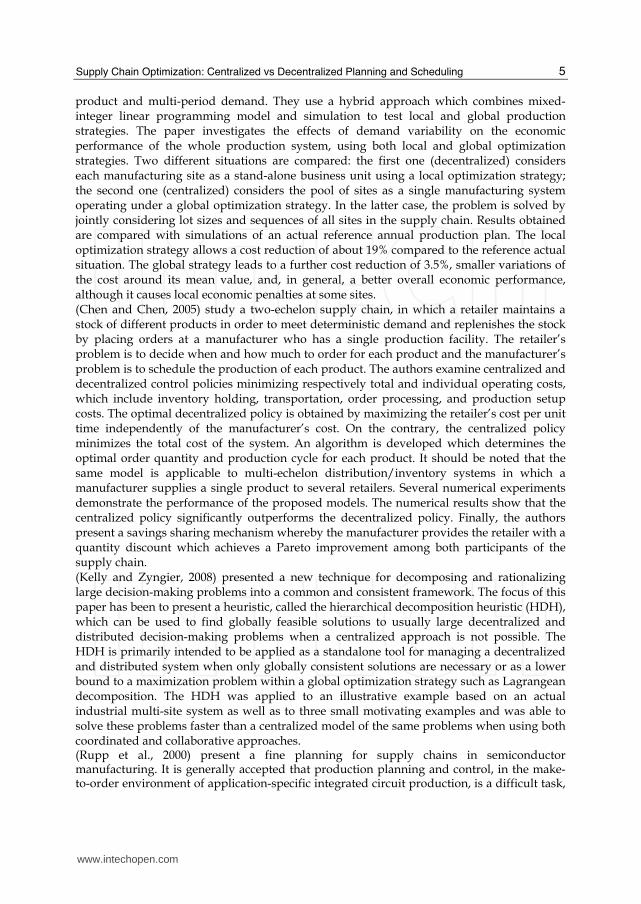
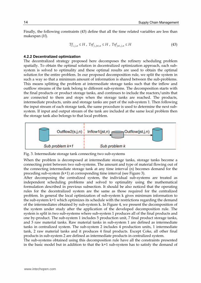
4.2.2 Decentralized optimization The decentralized strategy proposed here decomposes the refinery scheduling problem spatially. To obtain the optimal solution in decentralized optimization approach, each sub-system is solved to optimality and these optimal results are used to obtain the optimal solution for the entire problem. In our proposed decomposition rule, we split the system in such a way so that a minimum amount of information is shared between the sub-problems. This means splitting the problem at intermediate storage tanks such that the inflow and outflow streams of the tank belong to different sub-systems. The decomposition starts with the final products or product storage tanks, and continues to include the reactors/units that are connected to them and stops when the storage tanks are reached. The products, intermediate products, units and storage tanks are part of the sub-system 1. Then following the input stream of each storage tank, the same procedure is used to determine the next sub-system. If input and output stream of the tank are included at the same local problem then the storage tank also belongs to that local problem.

Fig. 3. Intermediate storage tank connecting two sub-systems

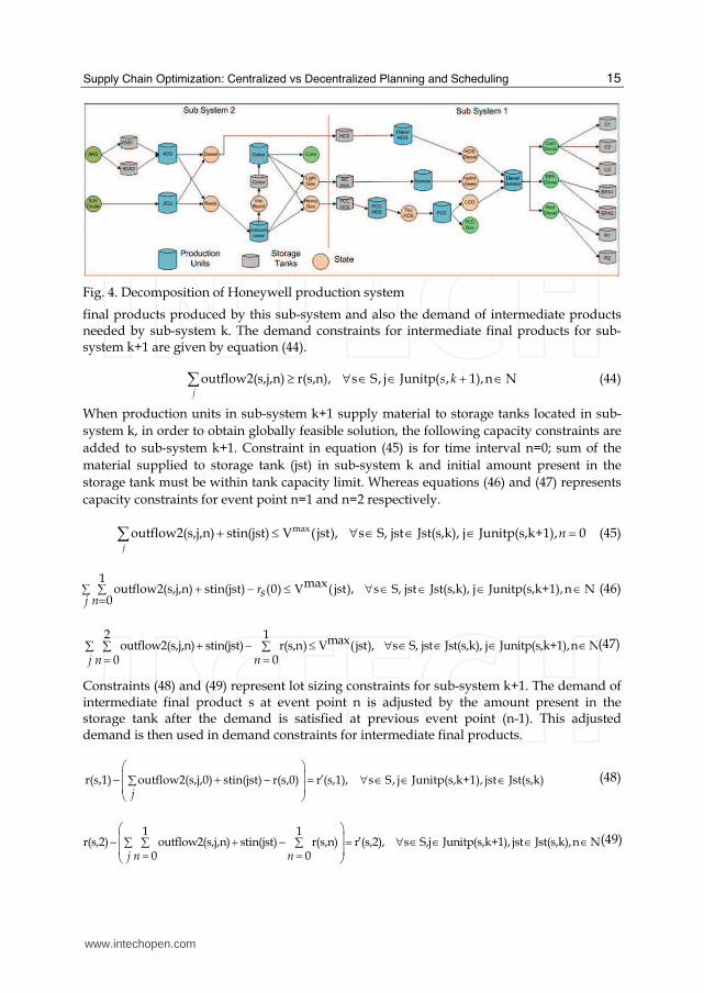
When the problem is decomposed at intermediate storage tanks, storage tanks become a connecting point between two sub-systems. The amount and type of material flowing out of the connecting intermediate storage tank at any time interval (n) becomes demand for the preceding sub-system (k+1) at corresponding time interval (see Figure 3). After decomposing the centralized system, the individual sub-systems are treated as independent scheduling problems and solved to optimality using the mathematical formulation described in previous subsection. It should be also noticed that the operating rules for the decentralized system are the same as those required for the centralized problem. In general the local optimization of sub-system k gives minimum information to the sub-system k+1 which optimizes its schedule with the restrictions regarding the demand of the intermediates obtained by sub-system k. In Figure 4, we present the decomposition of the system under study after the application of the developed decomposition rule. The system is split in two sub-systems where sub-system 1 produces all of the final products and one by-product. The sub-system 1 includes 5 production unit, 7 final product storage tanks, and 3 raw material tanks. Raw material tanks in sub-system 1 are defined as intermediate tanks in centralized system. The sub-system 2 includes 4 production units, 1 intermediate tank, 2 raw material tanks and it produces 4 final products. Except Coke, all other final products in sub-system 2 are defined as intermediate products in centralized system. The sub-systems obtained using this decomposition rule have all the constraints presented in the basic model but in addition to that the k+1 sub-system has to satisfy the demand of

www.intechopen.com


15

Fig. 4. Decomposition of Honeywell production system

final products produced by this sub-system and also the demand of intermediate products needed by sub-system k. The demand constraints for intermediate final products for sub-system k+1 are given by equation (44).

outflow2(s,j,n) r(s,n), s S, j Junitp( , 1),n Nj

s k≥ ∀ ∈ ∈ + ∈∑ (44)

When production units in sub-system k+1 supply material to storage tanks located in sub-

system k, in order to obtain globally feasible solution, the following capacity constraints are

added to sub-system k+1. Constraint in equation (45) is for time interval n=0; sum of the

material supplied to storage tank (jst) in sub-system k and initial amount present in the

storage tank must be within tank capacity limit. Whereas equations (46) and (47) represents

capacity constraints for event point n=1 and n=2 respectively.

maxoutflow2(s,j,n) stin(jst) V (jst), s S, jst Jst(s,k), j Junitp(s,k+1), 0j

n+ ≤ ∀ ∈ ∈ ∈ =∑ (45)

1 maxoutflow2(s,j,n) stin(jst) (0) V ( jst), s S, jst Jst(s,k), j Junitp(s,k+1),n N0

rsnj

+ − ≤ ∀ ∈ ∈ ∈ ∈∑ ∑= (46)

2 1 maxoutflow2(s,j,n) stin(jst) r(s,n) V (jst), s S, jst Jst(s,k), j Junitp(s,k+1),n N0 0j n n

+ − ≤ ∀ ∈ ∈ ∈ ∈∑ ∑ ∑= =(47)

Constraints (48) and (49) represent lot sizing constraints for sub-system k+1. The demand of intermediate final product s at event point n is adjusted by the amount present in the storage tank after the demand is satisfied at previous event point (n-1). This adjusted demand is then used in demand constraints for intermediate final products.

r(s,1) outflow2(s,j,0) stin(jst) r(s,0) r (s,1), s S, j Junitp(s,k+1), jst Jst(s,k)j

⎛ ⎞⎜ ⎟ ′− + − = ∀ ∈ ∈ ∈∑⎜ ⎟⎝ ⎠ (48)

1 1r(s,2) outflow2(s,j,n) stin(jst) r(s,n) r (s,2), s S,j Junitp(s,k+1), jst Jst(s,k),n N

0 0j n n

⎛ ⎞⎜ ⎟ ′− + − = ∀ ∈ ∈ ∈ ∈∑ ∑ ∑⎜ ⎟= =⎝ ⎠(49)

www.intechopen.com


16

The optimal time horizon of global problem is obtained by combining the optimal schedules

of sub-systems at each point (n) such that the material balance constraints are satisfied for

connecting intermediate storage tanks. Since sub-system k+1 satisfies the demand of sub-

system k, sub-system k+1 will happen before the sub-system k.

4.3 Qualitative results

In this section an analytical proof is presented in order to demonstrate that the

decentralization of the system under study using the rule presented in section 4.2.2 gives

exactly the same optimal makespam as the one obtained by centralized optimization. Proof: The makespam (HL: local makespam and HG: global makespam) is defined as follow:

,,

k

k

k zk z

H HH= ∑ where , , ,, ,,

( )k

f sk z i j ni j n

i n

HH T T= −∑ corresponds to zth group of kth sub-system.

The zth group is a group where all the j which belong to the zth group happen at the same time due to continuity of process operations. In the system under study applying the decomposition rule, we have 2 sub-systems which means k=2. For the 1st sub-system (k=1), z1=1,2 which means that we have 2 groups of units which do not operate at the same time (because of the coker tank). For the 2nd sub-system (k=2) all the units work at the same time z2=1. For z1=1: Vacum_tower, 2CU and 4CU, for z1=2: Coker and for z2=1: FCC HDS,

Isomax, FCC, Diesel HDS and Blender. If all the members of the sum ,,

k

k

k zk z

H HH= ∑ in

decentralized and centralized optimization are equal then L GH H= .

Without loss of generality, we are going to prove that for k=2 and z2=1 the centralized and

decentralized optimization gives the same optimal makespam. The same procedure can be

used to prove the case of k=1 and z1=1, 2.

We have to prove that for i,j which belong to z2=1, the equality 50 is valid:

, , , ,, , , ,, ,

( ) ( )f fs si j n i j ni j n i j n

i n i nL G

T T T T− = −∑ ∑ (50)

Proof of (50): If , , , ,i j n i j nn nL G

b b=∑ ∑ (51) then the equality (50) is valid ( 2,1 2,1L GHH HH= for

appropriate i,j). From constraints (34) we have for the decentralized model (34L) and centralized model (34G):

, , , , , , , ,, , , ,( ) ( )f fMIN s MAX si j L i j nL i j nL i j L i j nLi j n i j nR T T b R T T− ≤ ≤ − (34L)

, , , , , , , ,, , , ,( ) ( )f fMIN s MAX si j G i j nG i j nG i j G i j nGi j n i j nR T T b R T T− ≤ ≤ − (34G)

We sum (34L, 34G) over n and we get the following:

, , , , , , , ,, , , ,( ) ( )f fMIN s MAX si j L i j nL i j nL i j L i j nLi j n i j n

n n n

R T T b R T T− ≤ ≤ −∑ ∑ ∑ (34L')

, , , , , , , ,, , , ,( ) ( )f fMIN s MAX si j G i j nG i j nG i j G i j nGi j n i j n

n n n

R T T b R T T− ≤ ≤ −∑ ∑ ∑ (34G ')

We then make the following steps: (31L'-31G ') and (31G '-31L') and using (51) we prove (50).

www.intechopen.com


17

Proof of (51): In general only one unit j produces a product s. Thus, in constraints (33) only

one of the two parts exists because a product s is produced by a unique unit or is unloaded

from a tank or sum of tanks.

,,

1s

jst n sjst JST n

outflow r∈

≥∑ { }11,12,13s∈ (33A)

, ,,

2s j n sj n

outflow r≥∑ { }10,14s∈ (33B)

In decentralized and centralized optimization demand sr is the same which means that:

{ }, ,, ,

1 1 11,12,13s s

jst n jst njst JST n jst JST nL G

outflow outflow s∈ ∈

= ∈∑ ∑ (52)

{ }, , , ,, ,

2 2 10,14s j n s j nj n j nL G

outflow outflow s= ∈∑ ∑ (53)

We can obtain (52) and (53) by subtracting (33AL-33AG) and (33AG-33AL) where (33AL),

(33AG) are constraints (33A) for the decentralized and centralized case, respectively for (52)

and (33BL-33BG) and (33BG-33BL) (where (33BL), (33BG) are constraints (33B) for the

decentralized and centralized case) respectively for (53). It should be pointed out that the

sum over j in (53) can be eliminated because only one j produces the product s.

A general constraint of the system is that the production and the storage of a produced

product take place in the same time.

That means that: , , ,, ,

1 2s s

jst n s j njst JST n j n

outflow outflow∈

=∑ ∑ and eliminating the sum over j for the

same reason as in (53) we take: , , ,,

1 2s

jst n s j njst JST n n

outflow outflow∈

=∑ ∑ (54) for { }11,12,13s∈

and sj J∈ which is unique. From (53) and (54) we take:

{ }, , , ,2 2 , 10,11,12,13,14s j n s j nn nL G

outflow outflow s= ∈∑ ∑ (55). Let’s then consider the problem

constraints (31): { }, , , ,, 2 10,11,12,13,14j

pi j n s j ns i

i I

p b outflow s∈

= ∈∑ . Using constraints (27) only

one i happens at j in a certain period n. Then the sum over i can be relaxed:

{ }, , , ,, 2 10,11,12,13,14pi j n s j ns ip b outflow s= ∈ (56). Equation (56) is for the specific s which is

produced from a unique j from exact task i in a certain period n. Using equation (55) we have:

, , , ,2 2s j n s j nn nL G

outflow outflow=∑ ∑ ⇒ using (56) ⇒

, , , ,, ,p p

i j n i j ns i s in nL G

p b p b=∑ ∑ ⇒ , , , ,i j n i j nn nL G

b b=∑ ∑ ⇒

, , , ,, , , ,( ) ( )f fs si j n i j ni j n i j n

n nL G

T T T T− = −∑ ∑ ⇒ , , , ,, , , ,, ,

( ) ( )f fs si j n i j ni j n i j n

i n i nL G

T T T T− = −∑ ∑{ }, , 10,11,12,13,14j si I j J s∀ ∈ ∈ ∈ .

www.intechopen.com


18

That means that equality (50) is satisfied. Summarizing the presented proof is based on the fact that the total time needed to produce a group of products which are produced in the same period in units j of z group is the same in local and global optimization ■

5. Centralized vs decentralized control policies: A case study of aluminium doors with stochastic demand

5.1 Problem description

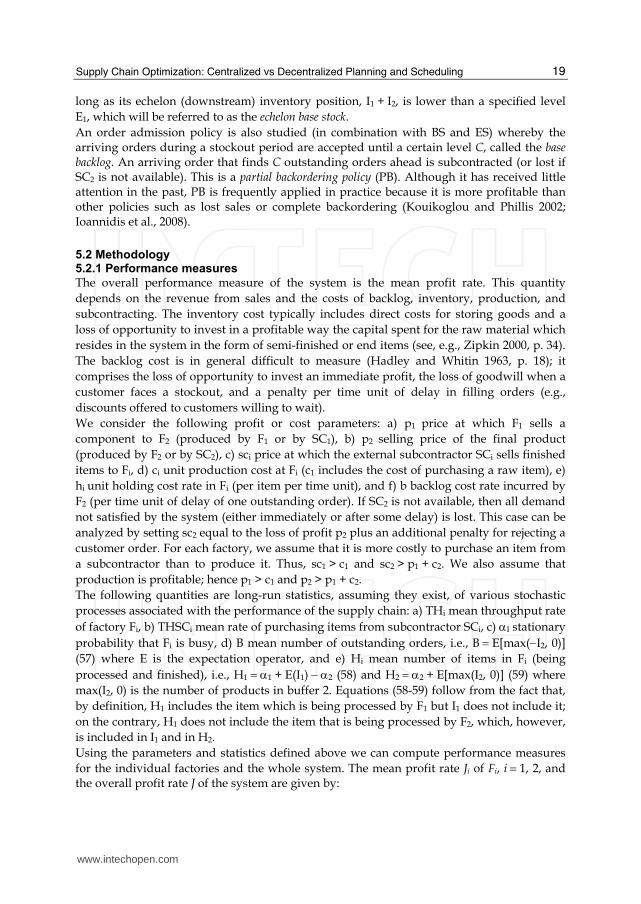
In this session, we examine a stochastic supply chain which corresponds at ANALKO enterprise. This supply chain is composed by two manufacturers that produce a single product type. The first manufacturer provides the basic component of the final product, and the second one makes the final product (see figure 4). Factory F1 purchases raw material, produces the basic component of product and places its finished items at buffer 1. The second factory makes final products and stores them in buffer 2 in anticipation of future demand. The processing times in each factory have exponential distributions and demand is a Poisson process with a constant rate. There is ample supply of raw items before the first factory so that F1 is never starved. There are also two external suppliers, subcontractor SC1 and, possibly, subcontractor SC2. SC1 can provide basic components to F2 whenever buffer 1 becomes empty. Thus, F2 is also never starved. SC2 can satisfy the demand during stockouts; if SC2 is not available, then all demand during stockouts is lost. Demand is satisfied by the finished goods inventory, if buffer 2 is not empty, otherwise it is either backlogged or satisfied by SC2. Whenever a demand is backlogged, backorder costs are incurred. Holding costs are incurred for the items held in buffer 1 and buffer 2 as well as for those being processed by F1 and F2. The objective is to control the release of items from each factory and each subcontractor to the downstream buffer so that the sum of the long-run average holding, backordering, and subcontracting costs is minimized. We use Markov chains to evaluate the performance of the supply chain under various control policies.

raw items factory F1

subcontractor SC1

buffer1

products

demand factory F2

subcontractor SC2

buffer2

FIRST COMPANY SECOND COMPANY

basic components

Fig. 4. The tow-stage supply chain of ANALKO

Let I1 denote the number of items in buffer 1 plus the item that is currently being processed

by F2, if any. Also, I2 is the inventory position of the second stage, that is, the number of

finished products in buffer 2 minus outstanding orders. Raw items that are being processed

by F1 are not counted in I1. The state variable I2 is positive when there are products in buffer

2; during stockout periods, I2 is negative, if there are outstanding orders to be filled, or zero

otherwise. Two production policies are examined: a) Base stock control (BS): Factory Fi, i = 1,

2, produces items whenever Ii is lower than a specified level Bi and stops otherwise. This

policy is commonly used in production systems, and b)Echelon base stock control (ES): Factory

F2 employs a base stock policy with threshold B2 as in BS, while F1 produces items only as

www.intechopen.com


19

long as its echelon (downstream) inventory position, I1 + I2, is lower than a specified level

E1, which will be referred to as the echelon base stock.

An order admission policy is also studied (in combination with BS and ES) whereby the arriving orders during a stockout period are accepted until a certain level C, called the base backlog. An arriving order that finds C outstanding orders ahead is subcontracted (or lost if SC2 is not available). This is a partial backordering policy (PB). Although it has received little attention in the past, PB is frequently applied in practice because it is more profitable than other policies such as lost sales or complete backordering (Kouikoglou and Phillis 2002; Ioannidis et al., 2008).

5.2 Methodology 5.2.1 Performance measures

The overall performance measure of the system is the mean profit rate. This quantity

depends on the revenue from sales and the costs of backlog, inventory, production, and

subcontracting. The inventory cost typically includes direct costs for storing goods and a

loss of opportunity to invest in a profitable way the capital spent for the raw material which

resides in the system in the form of semi-finished or end items (see, e.g., Zipkin 2000, p. 34).

The backlog cost is in general difficult to measure (Hadley and Whitin 1963, p. 18); it

comprises the loss of opportunity to invest an immediate profit, the loss of goodwill when a

customer faces a stockout, and a penalty per time unit of delay in filling orders (e.g.,

discounts offered to customers willing to wait).

We consider the following profit or cost parameters: a) p1 price at which F1 sells a

component to F2 (produced by F1 or by SC1), b) p2 selling price of the final product

(produced by F2 or by SC2), c) sci price at which the external subcontractor SCi sells finished

items to Fi, d) ci unit production cost at Fi (c1 includes the cost of purchasing a raw item), e)

hi unit holding cost rate in Fi (per item per time unit), and f) b backlog cost rate incurred by

F2 (per time unit of delay of one outstanding order). If SC2 is not available, then all demand

not satisfied by the system (either immediately or after some delay) is lost. This case can be

analyzed by setting sc2 equal to the loss of profit p2 plus an additional penalty for rejecting a

customer order. For each factory, we assume that it is more costly to purchase an item from

a subcontractor than to produce it. Thus, sc1 > c1 and sc2 > p1 + c2. We also assume that

production is profitable; hence p1 > c1 and p2 > p1 + c2.

The following quantities are long-run statistics, assuming they exist, of various stochastic

processes associated with the performance of the supply chain: a) THi mean throughput rate

of factory Fi, b) THSCi mean rate of purchasing items from subcontractor SCi, c) αI stationary

probability that Fi is busy, d) B mean number of outstanding orders, i.e., B = E[max(−I2, 0)]

(57) where E is the expectation operator, and e) Hi mean number of items in Fi (being

processed and finished), i.e., H1 = α1 + E(I1) − α2 (58) and H2 = α2 + E[max(I2, 0)] (59) where

max(I2, 0) is the number of products in buffer 2. Equations (58-59) follow from the fact that,

by definition, H1 includes the item which is being processed by F1 but I1 does not include it;

on the contrary, H1 does not include the item that is being processed by F2, which, however,

is included in I1 and in H2.

Using the parameters and statistics defined above we can compute performance measures

for the individual factories and the whole system. The mean profit rate Ji of Fi, i = 1, 2, and the overall profit rate J of the system are given by:

www.intechopen.com


20

J1 = (p1 − c1)TH1 + (p1 − sc1)THSC1 − h1H1 (60)

J2 = (p2 − c2 − p1)TH2 + (p2 − sc2)THSC2 − h2H2 − bB (61)

J = J1 + J2 (62)

In equations (57) and (58), the terms involving the throughput rates THi and THSCi represent net profits from sales of factory Fi. In equilibrium, the mean inflow rate of F2

equals its mean outflow rate, i.e., TH1 + THSC1 = TH2, and the mean demand rate equals TH2 + THSC2. If SC2 is not available, then THSC2 is the rate of rejected orders. Along with the policies BSPB and ESPB described in previous subsection, we consider two strategies the companies participating in ANALKO can adopt to maximize their profits: decentralized or local optimization and centralized or global optimization. In both cases, the objective is to determine C, B2, and B1 (under BSPB) or E1 (under ESPB) so as to maximize certain performance measures which are discussed next. Under decentralized optimization, factory F2 determines C and B2 which maximize its own profit rate J2. Recall that this factory is never starved. Therefore, regardless of the choice of B1 or E1, the second stage of the supply chain can be modeled as a single-stage queueing system in isolation in which the arrivals correspond to finished items leaving F2, the queue represents the products stored in buffer 2, and the departures correspond to customer orders. After specifying its control parameters, F2 communicates these values and also information about the demand to the first stage F1 which, in turn, seeks an optimal value for B1 or E1 so as to maximize J1. Under centralized optimization, the primary objective is to maximize the profit rate J of the system in all control parameters jointly. Intuitively, centralized optimization is overall more profitable than LO, i.e., JGO ≥ JLO. This can easily be shown by comparing the maximizing arguments (argmax) of profit equations. A general rule is that each company must benefit from being member of the supply chain. Under decentralized optimization, the second factory maximizes its own profit in an unconstrained manner, so J2LO ≥ J2GO. However, it follows from JGO ≥ JLO and (61) that J1GO ≥ J1LO. Thus, centralized optimization is more preferable than decentralized optimization for the first factory, provided that the second factory agrees to follow the same strategy. If the individual profits JiLO are acceptable for both factories, then LO could be used as a basis of a profit-sharing agreement: a) adopt centralized optimization, so that F1 accumulates more profit, and b) decrease the price p1 at which F1 sells to F2 so that, in the long run, factory Fi has a profit rate equal to JiLO plus a pre-agreed portion of the additional profit rate JGO − JLO. If, on the other hand, F1 is not willing to participate to a supply chain operating under decentralized optimization but it would be willing to do so under centralized optimization, then there are several possibilities for the two companies to reach (or not reach) a cooperation agreement, depending on the magnitude of the extra profit JGO − JLO and the profit margins of the company that owns F2. In general, such problems are difficult and often not well-posed because they are fraught with conflict of interests and subjectivity. In this paper, we assume that both companies are willing to adopt decentralized optimization, as is the case of ANALKO. The problem then is to investigate under which conditions the additional profit rate JGO − JLO would make it worth introducing centralized optimization and how the optimal control parameters can be computed.

5.2.2 Centralized and decentralized optimization

We assume that the processing times of F1 and F2 are independent, exponentially distributed

random variables with means 1/μi and the products are demanded one at a time according

www.intechopen.com


21

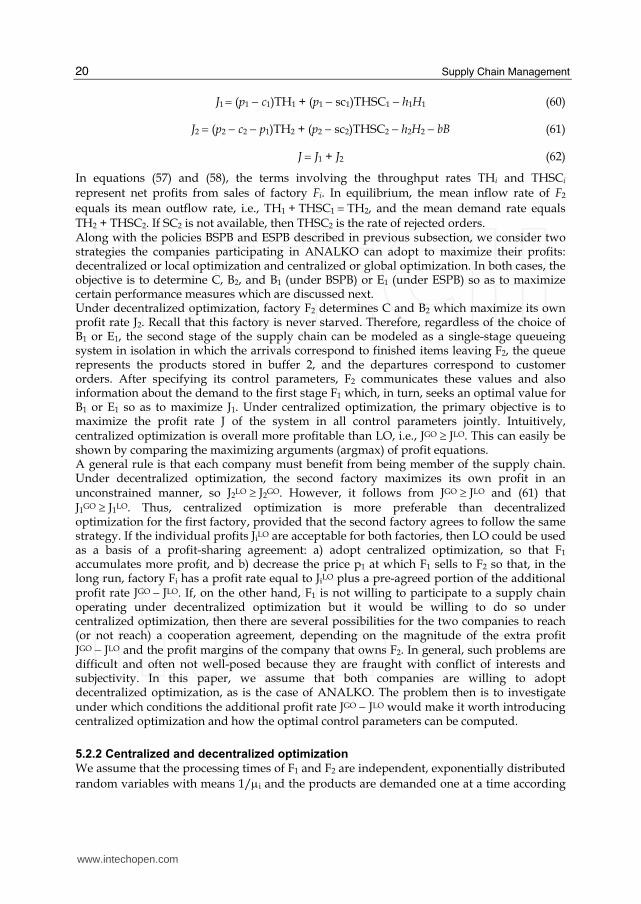
to a Poisson process with rate λ. In practice, the processing times often have lower variances than the exponential distribution. The assumption of exponential processing and interarrival times is adopted here in order to facilitate the analysis by Markov chain models. Systems with more general distributions can be evaluated using higher-dimensional Markovian models or simulation. The state of the system is the pair (I1, I2), i.e., the number of components which have not yet being processed by F2 and the inventory position of the second stage. The state variables provide information about the working status of each factory, and form a Markov chain whose dynamics depend on the production control policy as we shall discuss in the next two subsections. Modeling Base stock control with partial backordering: Factory F1 is working when I1 < B1.

Hence, a transition from state (I1, I2) to state (I1 + 1, I2) occurs with rate μ1, but these

transitions are disabled in states (B1, I2). A transition from state (I1, I2) to (I1 − 1, I2 + 1) occurs

with rate μ2 whenever I2 < B2. When I1 = 1, F2 is working on one item and buffer 1 is empty; in this case, if this item is produced before F1 sends another one to buffer 1, then the first company is obliged to deliver an item to F2 by purchasing one from SC1. We then have a

transition from state (1, I2) to (0, I2 + 1) with rate μ2, followed by an immediate transition to

(1, I2 + 1) which ensures that F2 will continue to produce. However, in state (1, B2 − 1), if F2 produces one item, then it stops producing thereafter since I2 reaches the base stock B2. Hence, there is no need to buy from SC1 and the new system state is (0, B2). Finally, we consider the state transitions triggered by a demand. According to the partial backordering

policy, an arriving customer order is rejected when I2 = −C, otherwise it is backordered and

the new state is I2 − 1. These transitions occur with rate λ. A diagram showing the state transitions explained above is shown in figure 5.

0, B2 1, B2 2, B2 B1 −1, B2 B1, B2

1, B2 −1 2, B2 −1 B1 −1,B2 −1 B1, B2 −1

1, −C+1 2, −C+1 B1 −1,−C+1 B1, −C+1

1, −C 2, −C B1 −1, −C B1, −C

1, −C+2 2, −C+2 B1 −1,−C+2 B1, −C+2

μ1

μ2

μ1

μ1

μ1 μ1 μ1

μ1

μ1

μ1

μ2

μ2

μ2

λ λ λ λ

λ λ λ λ

λ λ λ λ

μ2 μ2 μ2

μ2 μ2 μ2

μ2 μ2 μ2

μ2 μ2 μ2

λ λ λ λ

μ1

μ1

μ1

μ1

μ1

…

…

…

…

…

…

…

…

…

μ1 μ1

Fig. 5. Markov chain of the supply chain under BSPB.

The Chapman-Kolmogorov equations for the equilibrium probabilities P(I1, I2) are

I2 = B2: μ1P(0, B2) = μ2P(1, B2 − 1)

(λ + μ1)P(I1, B2) = μ1P(I1 − 1, B2) + μ2P(I1 + 1, B2 − 1) , 1 ≤ I1 ≤ B1 − 1,

λP(B1, B2) = μ1P(B1 − 1, B2)

B2 > I2 > −C: (λ + μ1 + μ2)P(1, I2) = μ2[P(1, I2 − 1) + P(2, I2 − 1)] + λP(1, I2 + 1)

www.intechopen.com


22

(λ + μ1 + μ2)P(I1, I2) = μ1P(I1 − 1, I2) + μ2P(I1 + 1, I2 − 1)

+ λP(I1, I2 + 1), 2 ≤ I1 ≤ B1 − 1,

(λ + μ2)P(B1, I2) = μ1P(B1 − 1, I2) + λP(B1, I2 + 1)

I2 = −C: (μ1 + μ2)P(1, −C) = λP(1, −C + 1)

(μ1 + μ2)P(I1, −C) = μ1P(I1 − 1, −C) + λP(I1, −C + 1), 2 ≤ I1 ≤ B1 − 1,

μ2P(B1, −C) = μ1P(B1 − 1, −C) + λP(B1, −C + 1).

We solve the first of the equations given above for P(0, B2) = (μ2/μ1)P(1, B2 − 1). We define

the column vectors PI2 = [P(1, I2) … P(B1, I2)]T for I2 = B2, B2 − 1, …, −C. The Chapman-

Kolmogorov equations can be written more compactly as:

A1PB2 = H1PB2−1 I2 = B2 (63)

API2 = GPI2+1 + HPI2−1 , I2 = B2 − 1, …, −C + 1 (64)

A0P−C = G0P−C+1, I2 = −C (65)

where A, A0, A1, H1, H, G, and G0 are matrices of suitable dimensions whose elements are the transition rates from and to the states of a given system level I2. This system of equations

can be solved sequentially: a) We solve equation (63) for PB2 = DB2PB2−1, where DB2 = A1−1H1,

b) then, we use the expression found in the previous iteration to solve equations (64) for

PI2 = DI2PI2−1, where DI2 = (A − GDI2+1)−1 and I2 = B2 − 1, B2 − 2, …, −C + 1, c) next, we

substitute P−C+1 = D−C+1P−C into equation (65) and compute P−C using the normalization

condition P(0, B2) +1 2

1 2

1 21

( , )B B

I I C

P I I= =−∑ ∑ = (μ2/μ1)P(1, B2 − 1) +

1 2

1 2

1 21

( , )B B

I I C

P I I= =−∑ ∑ = 1, and d)

finally, we compute the remaining probability vectors recursively from PI2 = DI2PI2−1, for

I2 = −C + 1, …, B2. From the equilibrium probabilities we can compute all the terms of

equations (60)−(62). We have:

THi = μiαi, THSC2 = λ − TH2, THSC1 = TH2 − TH1,

α1 = P(I1 < B1) = 1 − 2

2

1 2( , )B

I C

P B I=−∑ , α2 = P(I2 < B2) = 1 − 1

1

1 20

( , )B

I

P I B=∑ ,

E(I1) = 1

1 2

1 1 21 1

( , )B C

I I

I P I I−

= =∑ ∑ , E[max(−I2, 0)] = 1

2 1

2 1 21 1

( , )BC

I I

I P I I−=− =

⎡ ⎤− ⎢ ⎥⎢ ⎥⎣ ⎦∑ ∑ ,

E[max(I2, 0)] = B2P(0, B2) +2 1

2 1

2 1 21 1

( , )B B

I I

I P I I= =⎡ ⎤⎢ ⎥⎢ ⎥⎣ ⎦∑ ∑ .

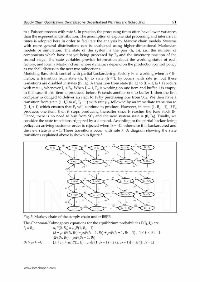
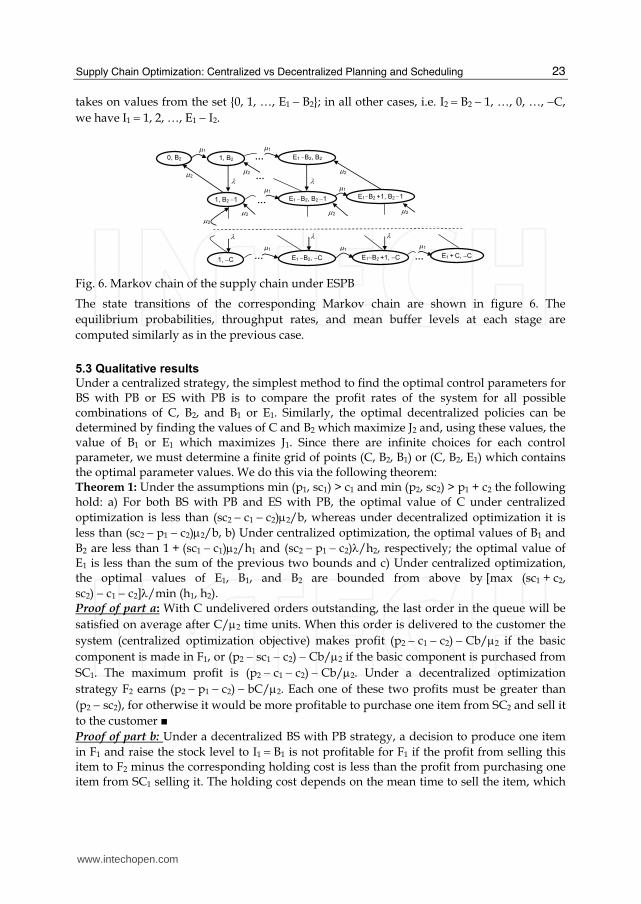
Upon substituting these quantities into equations (60)−(62) we compute J1, J2, and J. Modeling Echelon base stock control with partial backordering: The Markov chain has a

similar structure as previously, except that the maximum value of I1 is E1 − I2; so it is not

constant but it depends on the inventory position I2 of the second stage. When I2 = B2, I1

www.intechopen.com


23

takes on values from the set {0, 1, …, E1 − B2}; in all other cases, i.e. I2 = B2 − 1, …, 0, …, −C,

we have I1 = 1, 2, …, E1 − I2.

0, B2 1, B2 E1 −B2, B2

1, B2 −1 E1 −B2, B2 −1

1, −C E1 −B2, −C

μ1

μ2

μ2

λ λ

μ2

μ2

λ λ

μ1

μ1

E1−B2 +1, B2 −1

μ2

μ2

E1 + C, −Cμ1

E1−B2 +1, −C

λ

μ2

μ1

μ1 μ1

…

…

… …

…

Fig. 6. Markov chain of the supply chain under ESPB

The state transitions of the corresponding Markov chain are shown in figure 6. The

equilibrium probabilities, throughput rates, and mean buffer levels at each stage are

computed similarly as in the previous case.

5.3 Qualitative results

Under a centralized strategy, the simplest method to find the optimal control parameters for BS with PB or ES with PB is to compare the profit rates of the system for all possible combinations of C, B2, and B1 or E1. Similarly, the optimal decentralized policies can be determined by finding the values of C and B2 which maximize J2 and, using these values, the value of B1 or E1 which maximizes J1. Since there are infinite choices for each control parameter, we must determine a finite grid of points (C, B2, B1) or (C, B2, E1) which contains the optimal parameter values. We do this via the following theorem: Theorem 1: Under the assumptions min (p1, sc1) > c1 and min (p2, sc2) > p1 + c2 the following hold: a) For both BS with PB and ES with PB, the optimal value of C under centralized

optimization is less than (sc2 − c1 − c2)μ2/b, whereas under decentralized optimization it is

less than (sc2 − p1 − c2)μ2/b, b) Under centralized optimization, the optimal values of B1 and

B2 are less than 1 + (sc1 − c1)μ2/h1 and (sc2 − p1 − c2)λ/h2, respectively; the optimal value of E1 is less than the sum of the previous two bounds and c) Under centralized optimization, the optimal values of E1, B1, and B2 are bounded from above by [max (sc1 + c2,

sc2) − c1 − c2]λ/min (h1, h2). Proof of part a: With C undelivered orders outstanding, the last order in the queue will be

satisfied on average after C/μ2 time units. When this order is delivered to the customer the

system (centralized optimization objective) makes profit (p2 − c1 − c2) − Cb/μ2 if the basic

component is made in F1, or (p2 − sc1 − c2) − Cb/μ2 if the basic component is purchased from

SC1. The maximum profit is (p2 − c1 − c2) − Cb/μ2. Under a decentralized optimization

strategy F2 earns (p2 − p1 − c2) − bC/μ2. Each one of these two profits must be greater than

(p2 − sc2), for otherwise it would be more profitable to purchase one item from SC2 and sell it

to the customer ■

Proof of part b: Under a decentralized BS with PB strategy, a decision to produce one item

in F1 and raise the stock level to I1 = B1 is not profitable for F1 if the profit from selling this item to F2 minus the corresponding holding cost is less than the profit from purchasing one item from SC1 selling it. The holding cost depends on the mean time to sell the item, which

www.intechopen.com


24

is at least (B1 − 1)/μ2, assuming that F2, which is currently processing the first of the B1 items,

will not idle thereafter. Hence, we must have (p1 − c1) − h1(B1 − 1)/μ2 > (p1 − sc1). Using the

same argument for the second stage, we obtain (p2 − p1 − c2) − h2B2/λ > (p2 − sc2). From these inequalities we obtain the first two bounds of part (b). Under a decentralized ES with PB

strategy, we have E1 = max (I1 + I2) ≤ max (I1) + max (I2); the right side of the inequality is less than the sum of the previous two bounds and this concludes the proof ■ Proof of part c: Under a centralized strategy, a decision to produce an item in F1 leads to a

profit (p2 − c1 − c2) and a holding cost which is greater than min(h1, h2)(I1 + I2)/λ, where

I1 + I2 is the total inventory of the system and 1/λ is a lower bound on the mean time to sell

the item (relaxing the requirement that the item which is produced in F1 will experience an

additional delay at F2). The decision to produce the item in F1 is not profitable if the net

profit is less than the worst-case outsourcing profit p2 − max (sc1 + c2, sc2). So we have

(p2 − c1 − c2) − min (h1, h2)(I1 + I2)/λ ≥ p2 − max (sc1 + c2, sc2) from which we obtain the

bound on E1 = max (I1 + I2) given in part (c). Moreover, since max (I1 + I2) ≥ max (Ii) = Bi,

i = 1, 2, the same bound is also valid for Bi ■

Concluding, Theorem 1 ensures that the search space of optimal control parameters is

bounded. For example, suppose the extra cost for outsourcing from SC2 is sc2 − c1 − c2 = 10%

of the unit selling price, min (h1, h2) = 1% of the unit selling price per time unit, the mean

demand rate is λ = 5 products per time unit, and it holds that sc2 ≥ sc1 + c2, i.e., buying products from SC2 is more expensive than buying components from SC1 and processing them in F2 to make products. Then, from part (c) of Theorem 1, the upper bound on the

echelon surplus and the stock level I1 is 10 × 5/1 = 50. This is the maximum dimension of the

probability vectors and the transition matrices in equations (60−62).

6. Conclusion

It is known that decentralized planning results in loss of efficiency with respect to centralized planning. It is, however, difficult to quantify the difference between the two approaches within the context of production planning, production scheduling and control policies. In this chapter this issue was investigated in the setting of a two plant series production system of aluminum doors and a petrochemical multi-stage system. We have explored a “locally optimized” production planning procedure of ANALKO company where the downstream plant optimizes its production plan and the upstream plant follows his requests. Then we compared this decentralized optimized approach with centralized optimization where a single decision maker plans the production quantities of the supply chain in order to minimize total costs. Using our qualitative results, we have proved under which condition the two approaches give the same optimal solution. Future research could focus on development of efficient profit distribution strategies in case of centralized optimization. A structure decomposition strategy and formulation is also presented for short-term scheduling of refinery operations. An analytical mathematical proof is given in order to demonstrate that both optimization strategies result in the same optimal solution when the developed structural decomposition technique is applied. An interesting direction for the future is to examine the solutions given from centralized and decentralized strategy under different objective functions, such as maximization of profit, minimization of the inventory in the tanks.

www.intechopen.com


25

Finally, we have presented some Markovian queueing models to support the task of

coordinated decision making between two factories in a supply chain, which produces items

to stock to meet random demand. During stockout periods, each factory can purchase end

items from subcontractors. Production and subcontracting decisions in each factory are

made according to pull control policies. From theoretical results, it appears that managing

inventory levels and backorders jointly achieves higher profit than independently

determined control policies. Upper bounds for the control parameters are given follow by

analytical mathematical proofs. The study of multi-item, stochastic supply chains could be

another research direction. Since an exact analysis of multistage and/or multi-item supply

chains is usually hopeless, the development of efficient simulation algorithms and the

improvement of the accuracy of existing approximate analytical methods are the subjects of

ongoing research.

7. Appendixes

Appendix A:

Variables: T: Time Horizon (12 months), ,i tP : Production in factory iF during period t, ,i tI :

Inventory of factory iF during period t, ,i tSC : Subcontracting of factory iF during period t,

Parameters: icp : production cost of factory iF , ih : inventory cost of factory iF , csci : cost of

subcontracted products for factory iF , td : the demand of the final product during period t.

Appendix B

Sets: I : Tasks. J :Reactors, JST :Tanks, S :Materials, N : Event points, jI :Tasks that can

happen in unit j, iIseq ′ : Tasks that follow task i ′ ( i ′ produces s product that will be

consumed by i), jstJstprod :Units that follow tank jst, jstJprodst : Units that are followed by

tanks jst, sJunitp : Units that can produce material s, sJunitc :Units that consume material s,

jJseq ′ : Units that follow unit j′ (no storage in between), sJST : Tanks that can store material

s, jJSTprodst :Tanks that follow unit j, jJSTstprodt : Tanks that are followed by unit j.

Parameters: min

, jiR , max

, jiR :Min and Max production rate for unit j for task i, max

jstV :Maximum

capacity of tank jst, ,ps jρ , ,

cs jρ : Proportion of material s produced, and consumed from task i,

sr : Demand for material s at the end of the time horizon.

Decision Variables: i,j,nwv : Binary variables for task i at time point n, i,j,nb : Amount of

material in task i at unit j at time n, i,j,nTs : Time that task i starts in unit j at event point n,

i,j,nTf Time that task in finishes in unit j at event point n, j,jst,nin : Binary variable for flow

from unit j to tank jst, j,jst,n inflow : Amount of material flow from unit j to storage tank jst,

j,jst,nTss : Time that material starts to flow from unit j to tank jst at event point n, j,jst,n Tsf :

Time that material finishes to flow from unit j to tank jst at event point n, jst,j,nout : Binary

variable for flow from tank jst to unit j, jst,j,n outflow : Amount of material flow from storage

tank jst to unit j, jst,j,n Tss : Time that material starts to flow from tank jst to unit j at event

point n, jst,j,nTsf : Time that material finishes to flow from tank jst to unit j at event point n,

jst,n inflow1 : Inflow of raw material to storage tank jst at event point n, jst,n outflow1 :

Outflow of final product from storage tank jst at event point n, s,j,ninflow2 : Inflow of raw

material s to unit j at event point n, s,j,noutflow2 : Outflow of final product s from unit j at

event point n, s,j,jj,nunitflow : Flow of material from unit j to unit jj for consumption, jst,n st :

Amount of material in tank jst at event point n.

www.intechopen.com


26

8. References

Bassett, M.H., Pekny, J., & Reklaitis, G. (1996). Decomposition Techniques for the Solution of

Large-Scale Scheduling Problems. American Institute of Chemical Engineers

Journal 42(12),3373-3387.

Chen, J.M., & Chen, T.H. (2005). The Multi-item Replenishment Problem in a Two-Echelon

Supply Chain: The Effect of Centralization versus Decentralization. Computers &

Operations Research 32,3191-3207.

Gnoni, M., Iavagnilio, R., Mossa, G., Mummolo, G., & Leva, A.D. (2003). Prodcution

Planning of a Multi-site Manufacturing System by Hybrid Modeling: A Case Study

From the Automotive Industry. International Journal of Production Economics

85,251-262.

Hadley, G., Whitin, T.M., (1963). Analysis of Inventory Systems. Prentice Hall, Englewood

Cliffs, NJ.

Harjunkoski, I., & Grossmann, I.E. (2001). A Decomposition Approach For the Scheduling of

a Steel Plant Production. Computers and Chemical Engineering 25,1647-1660.

Ioannidis, S., Kouikoglou, V.S., Phillis, Y.A., (2008). Analysis of admission and inventory

control policies for production networks. IEEE Transactions on Automation Science

and Engineering, 5(2), 275–288.

Kelly, J.D., & Zyngier, D., (2008). Hierarchical Decomposition Heuristic for Scheduling:

Coordinated Reasoning for Decentralized And Distributed Decision-Making

Problems. Computers and Chemical Engineering 32: 2684-2705.

Kouikoglou, V.S., Phillis, Y.A., (2002). Design of product specifications and control policies

in a single-stage production system. IIE Transactions, 34, 590–600.

Liberopoulos, G., Dallery, Y., (2000). A unified framework for pull control mechanisms in

multi-stage manufacturing systems. Annals of Operations Research, 93, 325–355.

Liberopoulos, G., Dallery, Y., (2003). Comparative modelling of mutli-stage production-

inventory control policies with lot sizing. International Journal of Production

Research, 41, 1273–1298.

Rupp, M., Ristic, T.M., (2000) Fine planning for supply chains in semiconductor

manufacture. J. Materials Processing Technology 107: 390–397.

Zipkin, P.H., (2000). Foundations of Inventory Management. McGraw-Hill, New York.

www.intechopen.com

Supply Chain ManagementEdited by Dr. pengzhong Li

ISBN 978-953-307-184-8Hard cover, 590 pagesPublisher InTechPublished online 26, April, 2011Published in print edition April, 2011

InTech EuropeUniversity Campus STeP Ri Slavka Krautzeka 83/A 51000 Rijeka, Croatia Phone: +385 (51) 770 447 Fax: +385 (51) 686 166www.intechopen.com

InTech ChinaUnit 405, Office Block, Hotel Equatorial Shanghai No.65, Yan An Road (West), Shanghai, 200040, China

Phone: +86-21-62489820 Fax: +86-21-62489821

The purpose of supply chain management is to make production system manage production process, improvecustomer satisfaction and reduce total work cost. With indubitable significance, supply chain managementattracts extensive attention from businesses and academic scholars. Many important research findings andresults had been achieved. Research work of supply chain management involves all activities and processesincluding planning, coordination, operation, control and optimization of the whole supply chain system. Thisbook presents a collection of recent contributions of new methods and innovative ideas from the worldwideresearchers. It is aimed at providing a helpful reference of new ideas, original results and practical experiencesregarding this highly up-to-date field for researchers, scientists, engineers and students interested in supplychain management.

How to referenceIn order to correctly reference this scholarly work, feel free to copy and paste the following:

Georgios K.D. Saharidis (2011). Supply Chain Optimization: Centralized vs Decentralized Planning andScheduling, Supply Chain Management, Dr. pengzhong Li (Ed.), ISBN: 978-953-307-184-8, InTech, Availablefrom: http://www.intechopen.com/books/supply-chain-management/supply-chain-optimization-centralized-vs-decentralized-planning-and-scheduling

Documents

109 ' # '7& *#1 & 8 - Opencdn.intechopen.com/pdfs-wm/15529.pdf · Supply Chain Optimization: Centralized vs Decentralized Planning ... Optimal control policies are ... Supply Chain