On-line Supplementary Appendix
(not for publication)
Ethnic Inequality∗
Alberto F. Alesina
Harvard University, and IGIER, NBER, and CEPR
Stelios Michalopoulos
Brown University, and NBER
Elias Papaioannou
London Business School, CEPR, and NBER
October 21, 2014
Abstract
The Supplementary Appendix is split into four parts. Section 1 reports descriptive
and summary statistics for the newly constructed measures reflecting inequality across
ethnic homelands, administrative units, and 25 x 25 decimal-degree boxes. Section 2
reports a comprehensive set of sensitivity checks examining the association between ethnic
inequality and cross-country comparative development. Section 3 gives further evidence
and robustness checks on the origins of ethnic inequality. Section 4 offers additional results
on the association between differences in geographic endowments across ethnic homelands,
contemporary ethnic inequality, and comparative development.
∗We thank two anonymous referees, the Editor, Harald Uhlig, and several colleagues for proposing many ofthe sensitivity checks reported in this Supplementary Appendix. We would like to thank Nathan Fleming for
superlative research assistance. A special thanks also to Sebastian Hohmann for carefully checking all elements
of our codes. All errors are our sole responsibility.
0
1 Descriptive Evidence
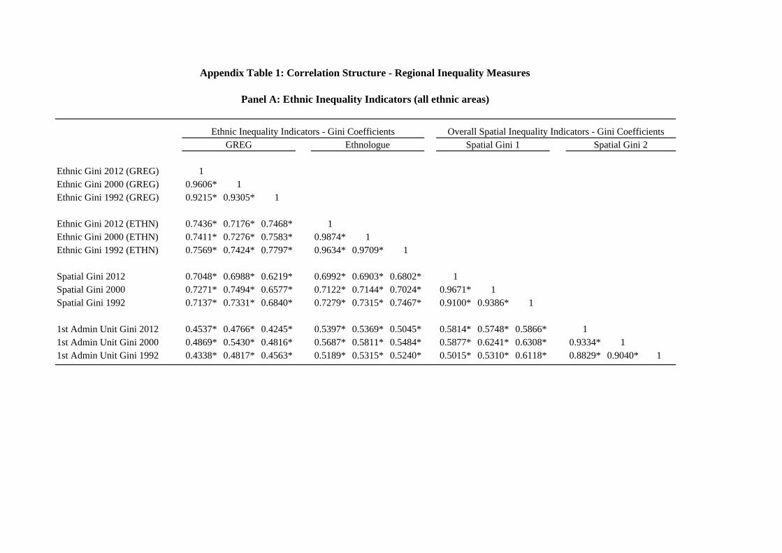
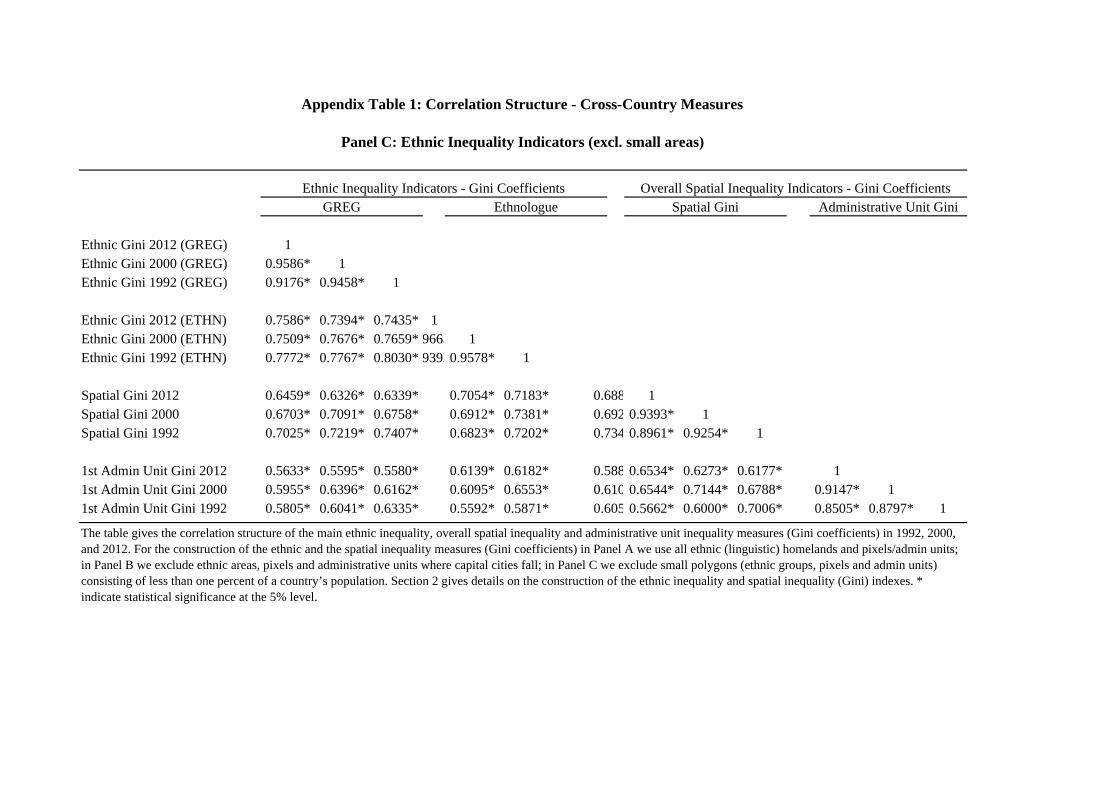
Appendix Table 1 reports the correlation structure between the newly constructed measures of
inequality across
1. ethnic groups based on the Atlas Narodov Mira (GREG),
2. linguistic groups using Ethnologue’s mapping,
3. pixels-boxes of 25 x 25 decimal degree ("virtual countries/homelands"), and
4. first-level administrative units.
The table gives the correlation matrix for three different points in time (1992, 2000 and
2012), and for three different sets of variables (samples). The first sample (Panel A), comprises
of all ethnic areas in each data set (GREG, Ethnologue, "virtual homelands/countries," and
first-level administrative units); the second sample (Panel B) excludes from the construction
of all inequality indexes areas where the capital cities fall; and the third sample (Panel C)
constructs Gini coefficients using data only from "large" polygons, i.e., those that constitute
at least 1% of the country’s population in 2000.
A couple of interesting patterns emerge. First, the correlation between the ethnic in-
equality proxies based on the Atlas Narodov Mira and Ethnologue is high, though far from
perfect (around 065 − 075). Second, all inequality measures (Gini coefficients) appear quitepersistent over time, although there has been some moderate decline in the past decade (see
Table 1).1 Third, the index capturing the overall degree of spatial inequality (based on boxes
of 25 x 25 decimal degrees) has a correlation coefficient with ethnic inequality (either based
on GREG or the Ethnologue) of roughly 070, whereas the respective statistic capturing the
correlation between ethnic inequality and inequality across first-level administrative units is
lower, around 040.
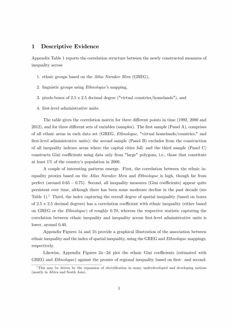
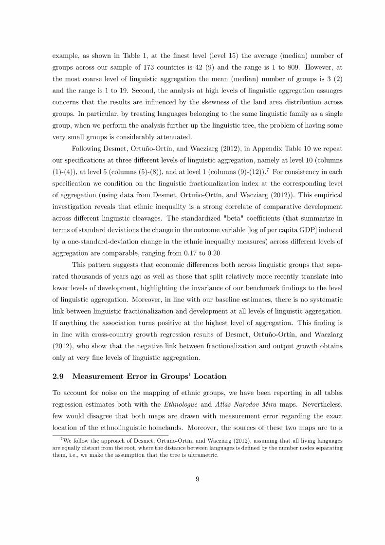
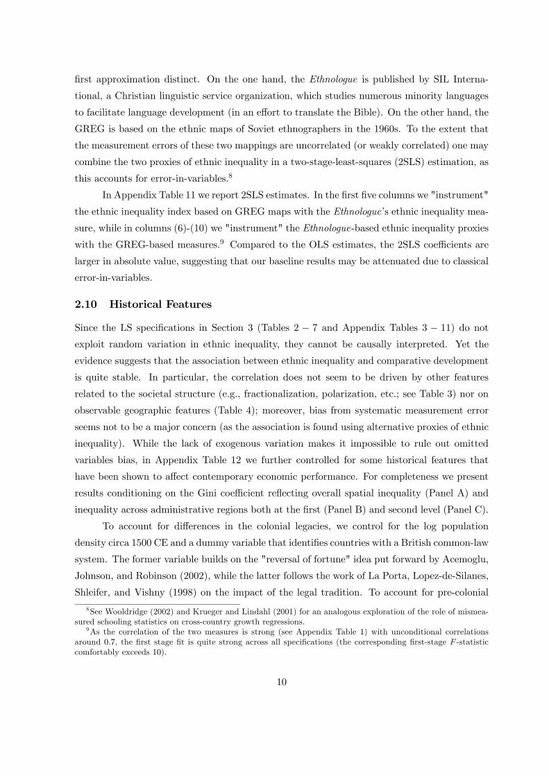
Appendix Figures 1a and 1b provide a graphical illustration of the association between
ethnic inequality and the index of spatial inequality, using the GREG and Ethnologue mappings,
respectively.
Likewise, Appendix Figures 2a−2d plot the ethnic Gini coefficients (estimated withGREG and Ethnologue) against the proxies of regional inequality based on first— and second-
1This may be driven by the expansion of electrification in many underdeveloped and developing nations
(mostly in Africa and South Asia).
1
level administrative units. There is an evident positive association; yet the correlation is far
from perfect.
AFG
AGO
ALB
ARE
ARG
ARM
ATG
AUS
AUT
AZE BDI
BEL
BEN BFA
BGDBGR
BHR BHS
BIHBLR
BLZ
BOLBRA
BRN
BTN
BWA
CAF
CAN
CHE
CHL
CHN
CIV
CMR
ZAR
COG
COL
COMCPV
CRI
CUB
CYP
CZE
DEU
DJI
DMA
DNK
DOM
DZA
ECU
EGYERI
ESP
EST
ETH
FIN
FJI
FRA
GAB
GBR
GEO
GHA
GIN
GMB
GNB GNQ
GRC
GRD
GTM
GUYHND
HRV
HTI
HUN
IDN
IND
IRL
IRN
IRQ
ISL
ISR
ITA
JAM
JOR
JPN
KAZ
KEN
KGZ
KHM
KNA KOR
KWT
LAO
LBN
LBR
LBY
LCA
LKA
LSO
LTU
LUX
LVA
MAR
MDA
MDG
MEXMKD
MLI
MLT
MNG
MOZ
MRT
MUS
MWI
MYS
NAM
NER
NGA
NIC
NLD
NOR
NPL
NZL
OMN
PAK
PAN
PER
PHL
PNG
POLPRT
PRY
QAT
ROM
RUS
RWA
SAU
SDN
SEN
SGP
SLBSLE
SLV
SOM
SUR
SVK
SVN
SWESWZ
SYC
SYR
TCD
TGO
THATJK
TKM
TON
TTO
TUN
TUR
TZA
UGA
UKR
URY
USA
UZB
VCT
VEN
VNM
VUTWSM
ZAF
ZMB
ZWE
0.0
00
0.2
00
0.4
00
0.6
00
0.8
00
1.0
00
Eth
nic
Ineq
ualit
y (G
ini C
oef
ficie
nt)
0.000 0.200 0.400 0.600 0.800 1.000Overall Spatial Inequality (Gini Coefficient)
Unc ond itional Relationship ( GRE G)
Ethnic Inequality and Spatial Inequality
Appendix Figure 1a
AFG AGO
ALB
ARE
ARG
ARMATG
AUS
AUT
AZE
BDI
BEL
BEN
BFA
BGD
BGR
BHR
BHS
BIH
BLR
BLZ
BOL
BRA
BRN
BTN
BWA
CAF
CAN
CHE
CHL
CHN
CIV
CMR ZARCOG
COL
COM
CPV
CRI
CUB
CYP
CZE
DEU
DJIDMA
DNK
DOM
DZA
ECU
EGY
ERI
ESP
EST
ETH
FIN
FJI
FRA
GAB
GBR
GEO
GHA
GIN
GMB
GNB
GNQ
GRC
GRD
GTM
GUY
HND
HRV HTI
HUN
IDN
IND
IRL
IRN
IRQ
ISL
ISRITA
JAM
JOR
JPN
KAZ
KEN
KGZ
KHM
KNA KOR
KWT
LAO
LBN
LBR
LBY
LCA
LKA
LSO
LTU
LUX LVA
MAR
MDA
MDG
MEX
MKD
MLI
MLT
MNG
MOZ
MRT
MUS
MWI
MYS
NAM
NERNGA
NIC
NLD
NOR
NPL
NZL
OMN
PAK
PAN
PER
PHL
PNG
POL
PRT
PRY
QAT
ROM
RUS
RWA
SAU
SDN
SEN
SGP
SLB
SLE
SLV
SOM
SUR
SVK
SVN
SWE
SWZSYC
SYR
TCD
TGO
THA
TJKTKM
TON
TTO
TUN
TUR
TZAUGA
UKR
URY
USA
UZB
VCT
VEN
VNM
VUT
WSM
ZAF
ZMB
ZWE
0.0
00
0.2
00
0.4
00
0.6
00
0.8
00
1.0
00
Eth
nic
Ineq
ualit
y (G
ini C
oef
ficie
nt)
0.000 0.200 0.400 0.600 0.800 1.000Overall Spatial Inequality (Gini Coefficient)
Uncond itional Relationship ( ETHNOLOGUE)
Ethnic Inequality and Spatial Inequality
Appendix Figure 1b
AFG
AGO
ALB
ARE
ARG
ARM
ATG
AUS
AUT
AZE BDI
BEL
BEN BFA
BGDBGR
BHR BHS
BIHBLR
BLZ
BOLBRA
BRN
BTN
BWA
CAF
CAN
CHE
CHL
CHN
CIV
CMR
ZAR
COG
COL
COM CPV
CRI
CUB
CYP
CZE
DEU
DJI
DMA
DNK
DOM
DZA
ECU
EGYERI
ESP
EST
ETH
FIN
FJI
FRA
GAB
GBR
GEO
GHA
GIN
GMB
GNB GNQ
GRC
GRD
GTM
GUYHND
HRV
HTI
HUN
IDN
IND
IRL
IRN
IRQ
ISL
ISR
ITA
JAM
JOR
JPN
KAZ
KEN
KGZ
KHM
KNA KOR
KWT
LAO
LBN
LBR
LBY
LCA
LKA
LSO
LTU
LUX
LVA
MAR
MDA
MDG
MEXMKD
MLI
MLT
MNG
MOZ
MRT
MUS
MWI
MYS
NAM
NER
NGA
NIC
NLD
NOR
NPL
NZL
OMN
PAK
PAN
PER
PHL
PNG
POLPRT
PRY
QAT
ROM
RUS
RWA
SAU
SDN
SEN
SGP
SLBSLE
SLV
SOM
SUR
SVK
SVN
SWESWZ
SYC
SYR
TCD
TGO
THATJK
TKM
TON
TTO
TUN
TUR
TZA
UGA
UKR
URY
USA
UZB
VCT
VEN
VNM
VUTWSM
ZAF
ZMB
ZWE
0.0
00
0.2
00
0.4
00
0.6
00
0.8
00
1.0
00
Eth
nic
Ineq
ualit
y (G
ini C
oef
ficie
nt)
0.000 0.200 0.400 0.600 0.800 1.000Inequality across Administrative Units, 1st-level (Gini Coef ficient)
Unc ond itional Relationship ( GRE G)
Ethnic Inequality and Inequality across Administrative Units
Appendix Figure 2a
AFG
AGO
ALB
ARGAUS
AUT
BDI
BEL
BEN BFA
BGDBGR
BIHBLR
BOLBRA
BRN
BTN
BWA
CAF
CAN
CHE
CHL
CHN
CIV
CMR
ZAR
COG
COLCRI
CUB
CZE
DEU
DJI
DNK
DOM
DZA
ECU
ERI
ESP
EST
ETH
FIN
FJI
FRA
GAB
GBR
GEO
GHA
GIN
GMB
GNB
GRC
GTM
GUYHND
HRV
HTI
HUN
IDN
IND
IRN
IRQ
ISL
ITA
JOR
JPN
KAZ
KEN
KHM
KOR
LAO
LBN
LBR
LKA
LTU
LUX
LVA
MAR
MDG
MEXMKD
MLI
MNG
MOZ
MRTMWI
MYS
NAM
NER
NGA
NIC
NLD
NOR
NPL
NZL
OMN
PAK
PAN
PER
PHL
PNG
POLPRT
PRY
RUS
RWA
SDN
SEN
SLE
SLV
SOM
SUR
SVK
SVN
SWE
SYR
TCD
TGO
THATJK
TUN
TUR
TZA
UGA
UKR
URY
USA
UZB
VEN
VNM
WSM
ZAF
ZMB
ZWE
0.0
00
0.2
00
0.4
00
0.6
00
0.8
00
1.0
00
Eth
nic
Ineq
ualit
y (G
ini C
oef
ficie
nt)
0.200 0.400 0.600 0.800 1.000Inequality across Administrative Units, 2nd-level (Gini Coefficient)
Unc ond itional Relationship ( GRE G)
Ethnic Inequality and Inequality across Administrative Units
Appendix Figure 2b
AFGAGO
ALB
ARE
ARG
ARM ATG
AUS
AUT
AZE
BDI
BEL
BEN
BFA
BGD
BGR
BHR
BHS
BIH
BLR
BLZ
BOL
BRA
BRN
BTN
BWA
CAF
CAN
CHE
CHL
CHN
CIV
CMR ZARCOG
COL
COM
CPV
CRI
CUB
CYP
CZE
DEU
DJIDMA
DNK
DOM
DZA
ECU
EGY
ERI
ESP
EST
ETH
FIN
FJI
FRA
GAB
GBR
GEO
GHA
GIN
GMB
GNB
GNQ
GRC
GRD
GTM
GUY
HND
HRV HTI
HUN
IDN
IND
IRL
IRN
IRQ
ISL
ISRITA
JAM
JOR
JPN
KAZ
KEN
KGZ
KHM
KNA KOR
KWT
LAO
LBN
LBR
LBY
LCA
LKA
LSO
LTU
LUXLVA
MAR
MDA
MDG
MEX
MKD
MLI
MLT
MNG
MOZ
MRT
MUS
MWI
MYS
NAM
NERNGA
NIC
NLD
NOR
NPL
NZL
OMN
PAK
PAN
PER
PHL
PNG
POL
PRT
PRY
QAT
ROM
RUS
RWA
SAU
SDN
SEN
SGP
SLB
SLE
SLV
SOM
SUR
SVK
SVN
SWE
SWZSYC
SYR
TCD
TGO
THA
TJK TKM
TON
TTO
TUN
TUR
TZAUGA
UKR
URY
USA
UZB
VCT
VEN
VNM
VUT
WSM
ZAF
ZMB
ZWE
0.0
00
0.2
00
0.4
00
0.6
00
0.8
00
1.0
00
Gin
i Eth
nic
Ine
qual
ity (
Gin
i Coe
ffic
ient
)
0.000 0.200 0.400 0.600 0.800 1.000Inequality across Adminisrative Regions, 1st -level (Gini Coefficient)
Uncond itional Relationship ( ETHNOLOGUE)
Ethnic Inequality and Inequality across Administrative Regions
Appendix Figure 2c
AFGAGO
ALB
ARG
AUS
AUT
BDI
BEL
BEN
BFA
BGD
BGR
BIH
BLR
BOL
BRA
BRN
BTN
BWA
CAF
CAN
CHE
CHL
CHN
CIV
CMR ZAR COG
COL
CRI
CUB
CZE
DEU
DJI
DNK
DOM
DZA
ECUERI
ESP
EST
ETH
FIN
FJI
FRA
GAB
GBR
GEO
GHA
GIN
GMB
GNB
GRC
GTM
GUY
HND
HRV HTI
HUN
IDN
IND
IRN
IRQ
ISL
ITA
JOR
JPN
KAZ
KEN
KHM
KOR
LAO
LBN
LBR
LKA
LTU
LUXLVA
MAR
MDG
MEX
MKD
MLIMNG
MOZ
MRT
MWI
MYS
NAM
NERNGA
NIC
NLD
NOR
NPL
NZL
OMN
PAK
PAN
PER
PHL
PNG
POL
PRT
PRYRUS
RWA
SDN
SEN
SLE
SLV
SOM
SUR
SVK
SVN
SWE
SYR
TCD
TGO
THA
TJK
TUN
TUR
TZAUGA
UKR
URY
USA
UZB
VEN
VNM
WSM
ZAF
ZMB
ZWE
0.0
00
0.2
00
0.4
00
0.6
00
0.8
00
1.0
00
Eth
nic
Ineq
ualit
y (G
ini C
oef
ficie
nt)
0.200 0.400 0.600 0.800 1.000Inequality across Adminisrative Regions, 2nd-level (Gini Coefficient)
Uncond itional Relationship ( ETHNOLOGUE)
Ethnic Inequality and Inequality across Administrative Regions
Appendix Figure 2d
2
In Appendix Table 2 we examine the association between the newly constructed measures
of ethnic and spatial inequality with (i) various measures of ethnic-linguistic diversity found
by previous research to be significant correlates of comparative development (Panel ) and (ii)
the level of economic development (as captured by the log of real GDP per capita in 2000)
and a Gini coefficient index capturing income inequality (Panel ).2 Panel reveals that
while the new measures of ethnic inequality correlate significantly with existing measures of
ethnic diversity, they capture something beyond this dimension, as the correlation coefficients
hover between 030 − 050. The correlation between the new proxies of ethnic inequality andethnic and linguistic segregation (Alesina and Zhuravskaya (2011)) or genetic diversity (Ashraf
and Galor (2013)) are lower (around 020). The ethnic inequality measures correlate strongly
(−050) with log GDP per capita, suggesting that under-development goes in tandem with an
unequal distribution of riches across ethnic homelands. In contrast, the correlation between
ethnic inequality and the standard measures (Gini coefficients) of income inequality is much
lower, around 020.
2 Ethnic Inequality and Economic Development
We have performed numerous sensitivity checks to explore the robustness of our finding in
Section 3 of the main part of the paper, showing a systematic negative association between
ethnic inequality and economic development across countries.
2.1 Baseline Estimates without Regional Fixed Effects
In all specifications in the main tables, we include a vector of region fixed effects (constants not
reported) so as to account for the sizable differences in comparative development and ethnic
inequality across these macro regions.3 Exploiting within-continent variation mitigates concerns
that the uncovered relationship is driven by differences in economic performance and ethnic
inequality across continents. Moreover, the inclusion of region-specific constants accounts for
measurement error in the underlying maps (Atlas Narodov Mira and Ethnologue) on the spatial
distribution of ethnic-linguistic groups around the world. For example, Ethnologue’s coverage
in Latin America is limited whereas it is extremely detailed for African countries.
As one may wonder whether or not accounting for these differences across regions changes
the observed pattern, we repeated estimation without including region fixed effects. In Appen-
dix Tables 3a and 3b we replicate the baseline specifications (reported in Tables 2a and 2b),
but omitting the region-specific constants. The association between cross-country comparative
2The Data Appendix lists detailed variable definitions and the respective sources.3 In our analysis, we follow World Bank’s regional classification.
3
development and ethnic inequality is quite strong. And while the overall degree of spatial in-
equality and fragmentation enter sometimes significantly, the regressions clearly point out that
it is inequality across ethnic homelands rather than the degree of spatial inequality or/and frac-
tionalization that is the key feature of under-development (columns (2)-(9)). For example, the
2 for the models associating log income per capita with the overall degree of spatial inequality
(column (3)) and fractionalization (column (5)) is 0176 and 011, respectively, much lower than
the analogous in-sample statistic with the ethnic inequality index (024). Moreover, compared
to the estimated coefficients in Tables 2a and 2b, the magnitude on the ethnic inequality in-
dex is quantitatively larger (most conservative estimates are −2 and −18 with GREG and
Ethnologue), suggesting that the cross-continental relationship between ethnic inequality and
comparative development is, if anything, stronger than the within-continent one we exploit in
the main part of the paper.
2.2 Alternative Measures of Ethnic Inequality in Different Samples
In Appendix Table 4, we report specifications linking the natural logarithm of GDP per capita
across countries to ethnic inequality when we exclude from the estimation both small in terms
of population groups and homelands that host the capital cities. By doing so the sample of
groups decreases substantially. For example, in the Atlas Narodov Mira when we exclude small
groups, 65% of the mapped ethnicities are not taken into account, whereas for the Ethnologue
the decline is even more dramatic; 82% of all mapped groups are less than 1% of their respective
countries’ populations and hence are not considered in the calculation of the ethnic Gini indexes.
The resulting set of groups further dwindles when we drop, on the top of relatively small
groups, those that host the capital cities (which may be multiple groups in few instances). This
additional restriction results in losing 25% of the cross-country sample, including countries like
Argentina or Armenia, for which there are no groups left to calculate ethnic Ginis for when these
two restrictions are put into place. So the sample is now limited to 130 countries. Interestingly,
even in this rather limited set of groups and countries economic disparities, as captured by
differences in luminosity per capita remain an inverse correlate of under-development. In Panel
we present specifications without continental fixed effects whereas in Panel we exploit
within-continent variation. We also control for inequality in group size (both in terms of
population and land area) to make sure that our estimates are not driven by differences in the
size across groups. Using the Ethnologue mapping the negative relationship between ethnic
inequality and comparative development is economically and statistically significant across all
specifications whereas using the Atlas Narodov Mira mapping the results are somewhat weaker,
though still the ethnic Gini index enters with a negative coefficient in all perturbations.
4
2.3 Excluding Single-Group Countries
In Appendix Table 5, we repeat the analysis, excluding countries that are populated by a single
ethnic (GREG) or linguistic (Ethnologue) group. In Panel we condition on the overall spatial
inequality index constructed using pixels-boxes of 25 x 25 decimal degrees, while in Panel
we control for inequality across first-level administrative units. To further examine the stability
of the estimates, we report results constructing inequality measures using all areas, dropping
areas where capitals fall, and dropping polygons of small ethnicities/boxes/administrative units
(defined as those with less than 1% of the country’s population). Across all permutations the
coefficient on the ethnic inequality (Gini) index is negative (around −1) and highly significant.This check explores the sensitivity of the association between ethnic inequality and comparative
development with respect to the intensive margin of ethnic diversity. The results suggest that,
looking at the latter, more ethnically unequal societies are also systematically less prosperous.
2.4 Using Radiance-Calibrated Levels of Luminosity
The underlying luminosity data are six-bit numbers ranging from 0 to 63.4 A concern of this
data series is the presence of top-coding which occurs in the urban cores of the developed
world. In these instances the ethnic inequality measures may be biased downward, especially
in rich countries with high urbanization (e.g., England, the US) where minorities (as defined
by GREG and the Ethnologue) are more likely to reside in less densely populated territories.
To account for saturation of recorded luminosity in very densely populated areas, we have
thus reconstructed all inequality measures, using as inputs the 2006 radiance-calibrated night-
time lights that do not suffer from top-coding, and repeated the empirical analysis. Appendix
Table 6 reports the results associating the log of real per capita GDP in 2006 with ethnic
inequality using the radiance-calibrated luminosity data. In Panel we condition on the index
capturing the overall degree of spatial inequality based on pixels of 25 x 25 degrees and in Panel
we condition on the Gini coefficient capturing inequality across first-level administrative
units. Using radiance-calibrated luminosity data has no material impact on our results. Across
all permutations the ethnic inequality measures enter with a significant coefficient, implying
that ethnic inequality is a key feature of under-development. Moreover, in line with our results
in the main part of the paper (Table 6-Panel ), inequality in development across first-level
administrative units is also a significant negative correlate of overall economic performance.
4For details on the luminosity data and some associated problems, see Henderson, Storeygard, and Weil
(2012), Chen and Nordhaus (2011), among others.
5
2.5 Accounting for the Resolution of the Raw Population Estimates
We also examined the robustness of our estimates to the quality of the underlying population
data used to construct the various inequality measures. The spatial resolution of the input
(usually census) polygons used to create the Gridded Population of the World (GPW) varies
across countries. The input polygons are subnational units (usually) at the administrative level
with a varying degree of resolution. The GPW does not model or reallocate the population,
but simply grids the data based on the original units at the smallest spatial size for which they
are available. For example, the GPW version 3 —that we use in estimating population across
different areas— uses a total of 399 747 subnational units as inputs around the world.
It is likely that states collecting fine-grained level population data are different in a variety
of dimensions compared to those that are not, for example, with respect to state capacity. An
inaccurate measure of population at the group level is likely to lead to mismeasured estimates
of luminosity per capita across groups potentially biasing our estimates. To mitigate such
concerns, we control for the coarseness of the GPW inputs units, augmenting the baseline
empirical model with the log of GPW "resolution" index. The resolution index can be thought
of as the average "cell size" for each country if all units in a country were square and of equal
size. The index is calculated as follows: Mean resolution in km = square root (country area
/ number of input units). Hence, a smaller “cell size,” i.e., a lower resolution, indicates a
higher quality of the underlying population estimates. Moreover, we constructed the mean
population density of each input unit as well as the number of subnational input units per
country. Conditional on the size and the total population of each country, these measures
provide alternative proxies for the quality of population data coverage.
In Appendix Table 7, we add these proxies of the coarseness of input units regard-
ing the construction of the population data sequentially to our specifications. Although in
some specifications some of these proxies of the underlying data quality enter with significant
point estimates,5 across all perturbations ethnic inequality enters with a precisely estimated
negative coefficient (range −08 − 12), suggesting that the underlying quality of the pop-ulation coverage is unlikely to be driving the observed association between ethnic inequality
and under-development. In line with our baseline estimates, the index of the overall degree
of spatial inequality enters with a negative though statistically insignificant coefficient (Panel
), further showing that it is inequality across ethnic homelands rather than the overall degree
of spatial inequality that correlates with underdevelopment. The Gini coefficient capturing
5For example, the resolution index enters with a negative (and in some permutations) significant coefficient,
implying that in countries with high quality population estimates (low resolution) development is higher. Like-
wise, the higher the number of administrative units used to compile the underlying population estimates, the
higher development is.
6
inequality in luminosity per capita across first-level administrative units enters with a nega-
tive and significant estimate (Panel ), suggesting that underdevelopment coevolves both with
ethnic inequality as well as inequality across politically defined units.
2.6 Using Alternative Local Population Estimates
The Gridded Population of the World (GPW) provides also an "adjusted" population density
at the grid level series. The difference between this and the simple (unadjusted) measure is
that for the adjusted population estimates at the grid level, the national-level populations from
the United Nations have been used to adjust the population estimates. While it is unclear
whether this adjustment reduces measurement error, and since in the benchmark tables we
use the non-adjusted population estimates, in Appendix Table 8 we report estimates using the
adjusted population series in the compilation of the inequality series in luminosity per capita.
As in our previous robustness checks, in Panel we condition on the overall spatial inequality
index based on 25 x 25 decimal degree boxes, while in Panel we account for inequality
across first-level administrative units. All our results remain intact. Across all specifications,
the ethnic inequality index enters with a statistically significant estimate. Moreover, there is
also a significant negative association between inequality across first-level administrative units
and income per capita.
2.7 Using Inequality Measures without Adjusting for Local Population
So far we have standardized luminosity of a homeland by its population to construct the
country-level Gini coefficients. In this section we show that we obtain a similar pattern when
we do not "standardize" light density by population, but account for differences in the size
of ethnic homelands, pixels/boxes, and administrative units, by independently controlling for
inequality in population and land area (as in Table 2). Using inequality in luminosity per square
kilometer is useful for at least two reasons. First, we allow for a flexible association between
development, luminosity, and population (without imposing any restriction a priori). Second,
these inequality measures are not contaminated by the measurement error induced from the
local population estimates. This approach is also closer to previous and parallel works that
use average luminosity per square kilometer in levels (without dividing by local population)
to proxy for development (e.g., Henderson, Storeygard, and Weil (2012), Hodler and Raschky
(2014), Fenske (2013), and Michalopoulos and Papaioannou (2013), among others).
Appendix Table 9 gives the results. For completeness we report estimates both with
the Atlas Narodov Mira mapping (columns (1)-(6)) and with the Ethnologue (columns (7)-
(1)2); using observations from all ethnic homelands, pixels/boxes, and administrative units
7
(in columns (1), (4), (7), and (10)), but also excluding areas where capitals fall (in (2), (5),
(8), and (11)) and small in terms of population areas (in (3), (6), (9), and (12)). Across all
permutations using the Ethnologue groups the ethnic Gini index enters with a robust negative
coefficient. The estimate (around −11 to −14) is also very similar to the baseline results(e.g., Tables 2− 5). The estimates associated with the Atlas Narodov Mira mappings are lessprecisely estimated and become insignificant when small groups are excluded.6 The coefficient
on the inequality measures capturing heterogeneity on the distribution of population (or land
area) across ethnic homelands is in most permutations statistically indistinguishable from zero
(coefficients not reported for brevity), further showing that it is inequality across ethnic lines in
economic performance rather than size (population and area) that correlates with country-level
development.
2.8 Ethnic Inequality at Different Levels of Linguistic Aggregation
One may wonder whether the inverse relationship between ethnic inequality and GDP per
capita is robust to alternative definitions of linguistic cleavages. We examined this issue in
detail. Our exploration is motivated by the informative work of Desmet, Ortuño-Ortín, and
Wacziarg (2012), who show that the effects of linguistic diversity on various political economy
outcomes (conflict, public goods, and economic growth) depend on the coarseness of linguistic
aggregation upon which diversity measures are based.
This sensitivity check is feasible in the context of the Ethnologue as we may trace the
entire linguistic tree of each group and hence we are able to aggregate languages at each
node. Ethnologue’s linguistic aggregation ranges from level 15, which is the finest one (and
the one we use in our baseline estimates), up to level 1, which is the coarsest level reporting
the macro family of each group. To put these different linguistic cleavages into perspective,
in our benchmark example (discussed in Section 2), Afghanistan has 39 groups at level 15 of
Ethnologue’s aggregation while there are only 4 groups at the coarsest level 1. Out of the 39
linguistic groups, 4 belong to the Altaic family, one to the Dravidian, one to the Afro-Asiatic,
and the rest to the Indo-European language family.
Besides exploring the role of ethnic inequality at various linguistic cleavages, performing
the analysis at higher levels of aggregation is useful for two additional reasons. First, we further
account for the fact that countries differ considerably in the number of linguistic groups. For
6A potential explanation for this pattern is the following. On the one hand, the Ethnologue maps the universe
of any documented language within a country (at least for the Old World). Hence, small groups in Ethnologue
may be extremely small and perhaps immaterial for understanding ethnic inequality in the country. On the other
hand, the Atlas Narodov Mira maps only a fourth of the groups compared to Ethnologue presumably the larger
and more important ones. This difference between the two mappings may explain why when dropping small
groups from the Ethnologue the estimated coefficients are largely unaffected whereas dropping small groups from
the Atlas Narodov Mira the resulting estimates become somewhat less precisely estimated.
8
example, as shown in Table 1, at the finest level (level 15) the average (median) number of
groups across our sample of 173 countries is 42 (9) and the range is 1 to 809. However, at
the most coarse level of linguistic aggregation the mean (median) number of groups is 3 (2)
and the range is 1 to 19. Second, the analysis at high levels of linguistic aggregation assuages
concerns that the results are influenced by the skewness of the land area distribution across
groups. In particular, by treating languages belonging to the same linguistic family as a single
group, when we perform the analysis further up the linguistic tree, the problem of having some
very small groups is considerably attenuated.
Following Desmet, Ortuño-Ortín, and Wacziarg (2012), in Appendix Table 10 we repeat
our specifications at three different levels of linguistic aggregation, namely at level 10 (columns
(1)-(4)), at level 5 (columns (5)-(8)), and at level 1 (columns (9)-(12)).7 For consistency in each
specification we condition on the linguistic fractionalization index at the corresponding level
of aggregation (using data from Desmet, Ortuño-Ortín, and Wacziarg (2012)). This empirical
investigation reveals that ethnic inequality is a strong correlate of comparative development
across different linguistic cleavages. The standardized "beta" coefficients (that summarize in
terms of standard deviations the change in the outcome variable [log of per capita GDP] induced
by a one-standard-deviation change in the ethnic inequality measures) across different levels of
aggregation are comparable, ranging from 017 to 020.
This pattern suggests that economic differences both across linguistic groups that sepa-
rated thousands of years ago as well as those that split relatively more recently translate into
lower levels of development, highlighting the invariance of our benchmark findings to the level
of linguistic aggregation. Moreover, in line with our baseline estimates, there is no systematic
link between linguistic fractionalization and development at all levels of linguistic aggregation.
If anything the association turns positive at the highest level of aggregation. This finding is
in line with cross-country growth regression results of Desmet, Ortuño-Ortín, and Wacziarg
(2012), who show that the negative link between fractionalization and output growth obtains
only at very fine levels of linguistic aggregation.
2.9 Measurement Error in Groups’ Location
To account for noise on the mapping of ethnic groups, we have been reporting in all tables
regression estimates both with the Ethnologue and Atlas Narodov Mira maps. Nevertheless,
few would disagree that both maps are drawn with measurement error regarding the exact
location of the ethnolinguistic homelands. Moreover, the sources of these two maps are to a
7We follow the approach of Desmet, Ortuño-Ortín, and Wacziarg (2012), assuming that all living languages
are equally distant from the root, where the distance between languages is defined by the number nodes separating
them, i.e., we make the assumption that the tree is ultrametric.
9
first approximation distinct. On the one hand, the Ethnologue is published by SIL Interna-
tional, a Christian linguistic service organization, which studies numerous minority languages
to facilitate language development (in an effort to translate the Bible). On the other hand, the
GREG is based on the ethnic maps of Soviet ethnographers in the 1960s. To the extent that
the measurement errors of these two mappings are uncorrelated (or weakly correlated) one may
combine the two proxies of ethnic inequality in a two-stage-least-squares (2SLS) estimation, as
this accounts for error-in-variables.8
In Appendix Table 11 we report 2SLS estimates. In the first five columns we "instrument"
the ethnic inequality index based on GREG maps with the Ethnologue’s ethnic inequality mea-
sure, while in columns (6)-(10) we "instrument" the Ethnologue-based ethnic inequality proxies
with the GREG-based measures.9 Compared to the OLS estimates, the 2SLS coefficients are
larger in absolute value, suggesting that our baseline results may be attenuated due to classical
error-in-variables.
2.10 Historical Features
Since the LS specifications in Section 3 (Tables 2 − 7 and Appendix Tables 3 − 11) do notexploit random variation in ethnic inequality, they cannot be causally interpreted. Yet the
evidence suggests that the association between ethnic inequality and comparative development
is quite stable. In particular, the correlation does not seem to be driven by other features
related to the societal structure (e.g., fractionalization, polarization, etc.; see Table 3) nor on
observable geographic features (Table 4); moreover, bias from systematic measurement error
seems not to be a major concern (as the association is found using alternative proxies of ethnic
inequality). While the lack of exogenous variation makes it impossible to rule out omitted
variables bias, in Appendix Table 12 we further controlled for some historical features that
have been shown to affect contemporary economic performance. For completeness we present
results conditioning on the Gini coefficient reflecting overall spatial inequality (Panel A) and
inequality across administrative regions both at the first (Panel B) and second level (Panel C).
To account for differences in the colonial legacies, we control for the log population
density circa 1500 CE and a dummy variable that identifies countries with a British common-law
system. The former variable builds on the "reversal of fortune" idea put forward by Acemoglu,
Johnson, and Robinson (2002), while the latter follows the work of La Porta, Lopez-de-Silanes,
Shleifer, and Vishny (1998) on the impact of the legal tradition. To account for pre-colonial
8See Wooldridge (2002) and Krueger and Lindahl (2001) for an analogous exploration of the role of mismea-
sured schooling statistics on cross-country growth regressions.9As the correlation of the two measures is strong (see Appendix Table 1) with unconditional correlations
around 07, the first stage fit is quite strong across all specifications (the corresponding first-stage -statistic
comfortably exceeds 10).
10
conditions, following Ashraf and Galor (2013) and Putterman and Weil (2010), we also control
for the log of the timing since the Neolithic revolution (ancestry adjusted) which takes into
account the experience of contemporary inhabitants within a country regarding the transition
to agriculture of their ancestors. Adding these historical controls has virtually no effect on
the estimates. The coefficient on the ethnic inequality index is more than two standard errors
below zero across all specifications. Moreover, the magnitude of the estimate is quite stable.
2.11 Regional Heterogeneity
The evidence produced so far points out that ethnic inequality is a robust and so far neglected
correlate of cross-country economic performance. While the inclusion of region-fixed effects en-
sures that our finding is not driven by continental differences in development and ethnic/spatial
inequality, it is interesting to examine whether some regions/continents are more important sta-
tistically than others in driving the association. For example, casual empiricism suggests that
ethnicity is more salient in Africa, the Middle-East, and Asia, as compared to Western Europe.
Moreover, in Europe and North America people of different groups often live in close proximity
whereas for Asian and African countries groups’ mixing is often low.
In Appendix Table 13 we examine the robustness of our findings when we drop iteratively
countries of each main (World Bank) region. In columns (1) and (7) we drop observations from
Western Europe and North America (USA and Canada). In columns (2) and (8) we exclude
countries from East Asia and the Pacific (EAP) and South Asia (SA). In specifications (3)
and (9) we do not consider countries in Sub-Saharan Africa. In columns (4) and (10) we drop
countries from the Middle East and North Africa region. In columns (5) and (11) we exclude
states from Eastern Europe and Central Asia, while in columns (6) and (12) we drop countries
in Latin America and the Caribbean. The coefficient on the ethnic inequality index is negative
and statistically significant across all permutations. This suggests that the main pattern we
have established so far is not driven by a single region. Nevertheless, a closer examination
reveals that the association between ethnic inequality and GDP per capita is stronger when we
drop Western Europe and North America and somewhat weaker when we drop Asian countries
and the Middle East and North Africa region.
More generally, one would expect our ethnic inequality index (as constructed) to be more
accurate for regions like Africa, the Middle East, and Asia where groups are more clearly de-
lineated and have little spatial overlap compared to countries in Western Europe and North
America where segregation along ethnic-linguistic lines is low. In Appendix Table 14 we ex-
amine the association between development and ethnic inequality within each region. While
the number of observations falls considerably —leading to imprecise estimates— there is clear
11
evidence that the relationship between ethnic inequality and GDP per capita is strongest for
countries in East and South Asia,10 the Middle East, and North Africa and Sub-Saharan Africa.
In contrast, the association is virtually non-existent for Western Europe and North America.
For countries in Eastern Europe and Central Asia, the association is negative but imprecisely
estimated whereas for Latin American countries, the correlation depends on the underlying
mapping of groups. Interestingly, when the GREG is used (which unlike Ethnologue reports
the location of immigrant languages that are the majority groups in Latin America today) there
is a negative and statistically significant association between ethnic inequality and comparative
development.
3 On the Origins of Ethnic Inequality
3.1 Colonial Origins
Given the strong correlation between ethnic inequality and income per capita, we tried identi-
fying the historical correlates of ethnic inequality, building on the literature assessing the legacy
of colonization on contemporary development. Appendix Table 15 reports the results. Ethnic
inequality does not seem to be driven by the legal framework that has been transplanted by col-
onizers (columns (1) and (6); see La Porta, Lopez-de-Silanes, Shleifer, and Vishny (1998)), the
type of colonization and colonial institutions as reflected in settler mortality (columns (2) and
(7); see Acemoglu, Johnson, and Robinson (2001)) or population density before colonization
(columns (3) and (8); see Acemoglu, Johnson, and Robinson (2002)), the share of Europeans
in the population (columns (4) and (9); see Hall and Jones (1999) and Putterman and Weil
(2010)), and ethnic partitioning and border artificiality (columns (5) and (10); see Alesina,
Easterly, and Matuszeski (2011)). These insignificant associations hint that the strong nega-
tive correlation between ethnic inequality and development does not reflect the role of colonial
history.11
3.2 Geographic Origins
As we show in Table 7, differences in geographic attributes across groups explain a sizeable
fraction of the variation in incomes across ethnic homelands (ethnic inequality). The geographic
10Since there are only 7 countries in South Asia (namely Afghanistan, Bangladesh, Bhutan, India, Nepal,
Pakistan, and Sri Lanka), we merge this region with the East Asia region that includes 21 countries (e.g.,
Indonesia, Japan, Cambodia, Lao, Mongolia, China, Malaysia).11There is also no systematic link between ethnic inequality and proxies of statehood (state antiquity index
of Bockstette, Chanda, and Putterman (2002)) or early national institutions (as proxied by the average value
of Polity’s executive constraints index in the first decade after independence, see Acemoglu, Johnson, Robinson,
and Yared (2008)).
12
features that we use in the main part of the paper are (average): land quality, temperature,
precipitation, distance to the coast, and elevation.
In Appendix Table 17, we augment the set of geographic variables, adding two more
attributes. Namely, the seasonality of temperature (measured as the difference between the
annual maximum and minimum temperatures) and variability (standard deviation) of precipi-
tation across ethnic homelands (Appendix Table 16 reports summary statistics). In line with
our results in the main part of the paper (Table 7), in most specifications the various geographic
Gini indicators enter with positive coefficients, suggesting that contemporary differences in de-
velopment across ethnic lines (as captured by per capita luminosity) have a sizable geographic
component. Regarding the new geographic covariates, inequality across ethnic homelands of
the variability of precipitation is not systematically linked to ethnic inequality. However, the
coefficient on the Gini index capturing inequality in temperature seasonality is positive and
significant in all permutations. In countries where the temperature range differs greatly across
ethnic territories, group inequality is also high. To the extent that a larger temperature range
allows for a wider set of crops to be cultivated this may be a channel via which inequality in
temperature seasonality may lead to differential economic performance across groups.12
3.3 A Composite Index of Geographic Inequality across Ethnic Homelands
based on a Richer Set of Variables
We investigated the robustness of our results in the second part of the paper (Section 4) link-
ing inequality in geographic endowments across ethnic regions to contemporary differences in
well-being across ethnic homelands (ethnic inequality) using a composite index that captures
geographic differences across these seven geographic traits (average land quality, mean temper-
ature, mean precipitation, distance to the coast, mean elevation, variability in precipitation,
and seasonality in temperature). As in Section 4 we extract the first principal component of
this richer set of geographic features and then examine its association with ethnic inequality.
The first principal component explains approximately 45% to 50% of the common variance of
the seven variables.
Using a richer set of geographic controls does not alter the pattern established in the
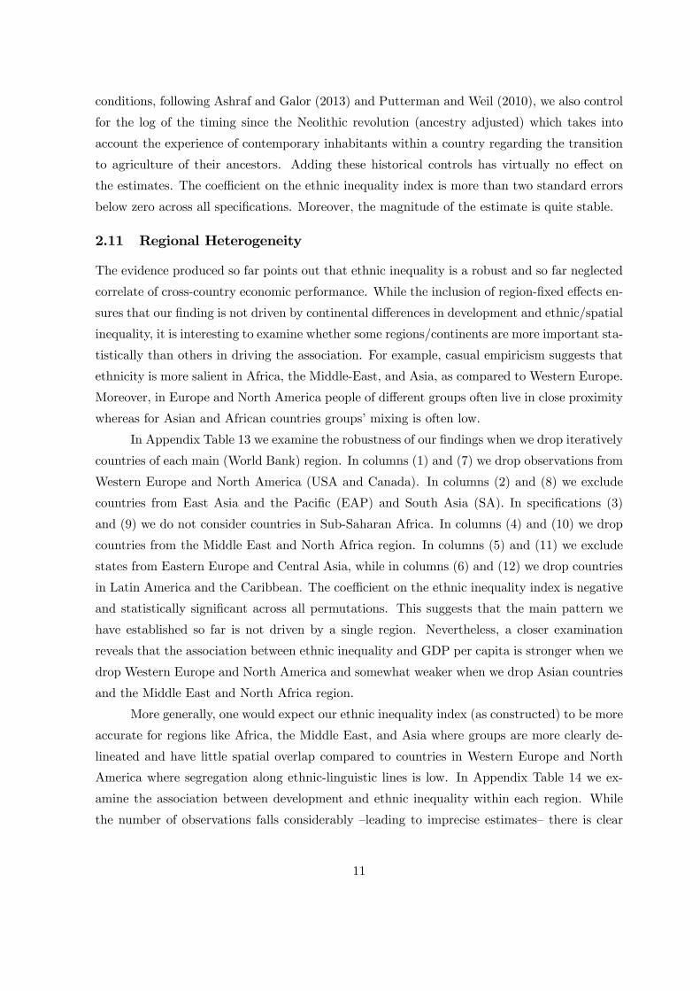
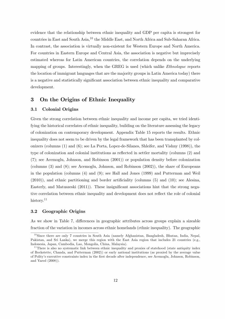
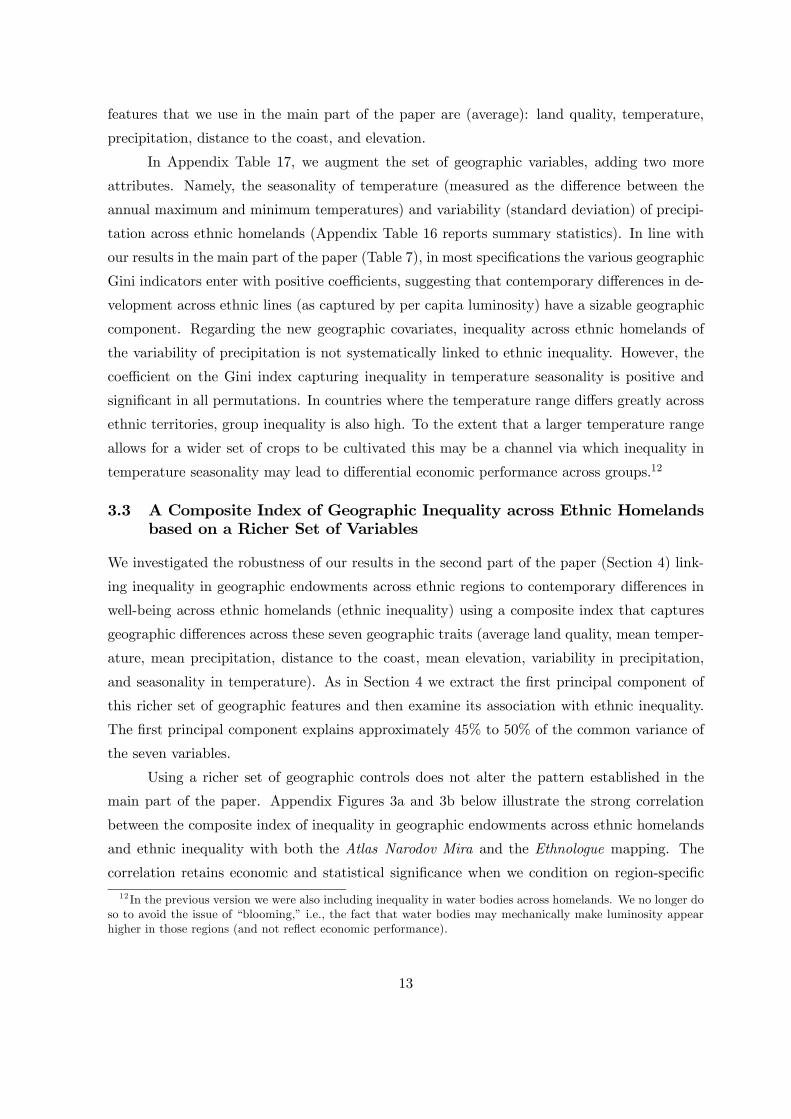
main part of the paper. Appendix Figures 3a and 3b below illustrate the strong correlation
between the composite index of inequality in geographic endowments across ethnic homelands
and ethnic inequality with both the Atlas Narodov Mira and the Ethnologue mapping. The
correlation retains economic and statistical significance when we condition on region-specific
12 In the previous version we were also including inequality in water bodies across homelands. We no longer do
so to avoid the issue of “blooming,” i.e., the fact that water bodies may mechanically make luminosity appear
higher in those regions (and not reflect economic performance).
13
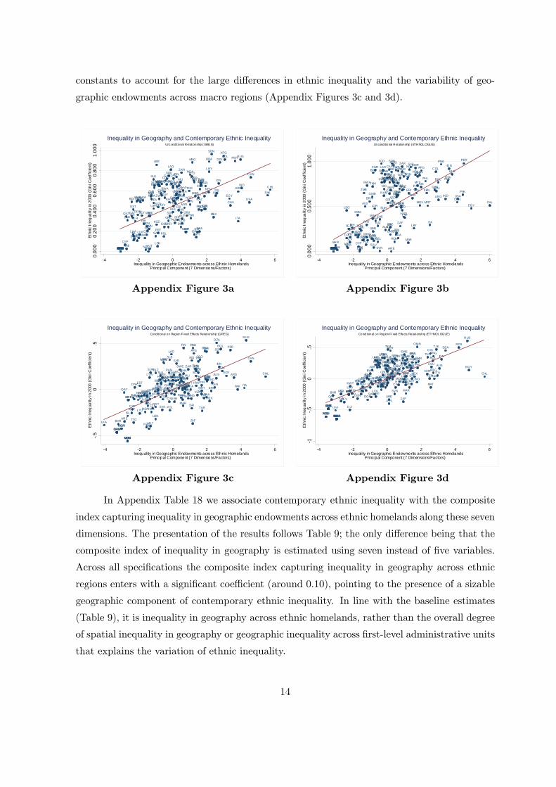
constants to account for the large differences in ethnic inequality and the variability of geo-
graphic endowments across macro regions (Appendix Figures 3c and 3d).
AFG
AGO
ALB
ARE
ARG
ARM
AUS
AUT
AZEBDI
BEL
BENBFA
BGDBGR
BHRBHS
BIHBLR
BLZ
BOLBRA
BRN
BTN
BWA
CAF
CAN
CHE
CHL
CHN
CIV
CMR
ZAR
COG
COL
COMCPV
CRI
CUB
CYP
CZE
DEU
DJI
DNK
DOM
DZA
ECU
EGYERI
ESP
EST
ETH
FIN
FJI
FRA
GAB
GBR
GEO
GHA
GIN
GMB
GNBGNQ
GRC
GTM
GUY HND
HRV
HTI
HUN
IDN
IND
IRL
IRN
IRQ
ISL
ISR
ITA
JAM
JOR
JPN
KAZ
KEN
KGZ
KHM
KOR
KWT
LAO
LBN
LBR
LBY
LKA
LSO
LTU
LUX
LVA
MAR
MDA
MDG
MEXMKD
MLI
MNG
MOZ
MRT
MUS
MWI
MYS
NAM
NER
NGA
NIC
NLD
NOR
NPL
NZL
OMN
PAK
PAN
PER
PHL
PNG
POLPRT
PRY
QAT
ROM
RUS
RWA
SAU
SDN
SEN
SGP
SLBSLE
SLV
SOM
SUR
SVK
SVN
SWESWZ
SYR
TCD
TGO
THATJK
TKM
TTO
TUN
TUR
TZA
UGA
UKR
URY
USA
UZB
VEN
VNM
VUTWSM
ZAF
ZMBZWE
0.0
00
0.2
00
0.4
00
0.6
00
0.8
00
1.0
00
Eth
nic
Ineq
ualit
y in
200
0 (
Gin
i Coe
ffic
ient
)
-4 -2 0 2 4 6Inequality in Geographic Endowments across Ethnic Homelands
Princ ipal Component (7 Dimensions/Factors)
Unc ond itional Relationship ( GRE G)
Inequality in Geography and Contemporary Ethnic Inequality
Appendix Figure 3a
AFGAGO
ALB
ARE
ARG
ARM
AUS
AUT
AZE
BDI
BEL
BEN
BFA
BGD
BGR
BHR
BHS
BIH
BLR
BLZ
BOL
BRA
BRN
BTN
BWA
CAF
CAN
CHE
CHL
CHN
CIV
CMRZARCOG
COL
COM
CPV
CRI
CUB
CYP
CZE
DEUDJI
DNK
DOM
DZA
ECU
EGY
ERI
ESP
EST
ETH
FIN
FJI
FRA
GAB
GBR
GEO
GHA
GIN
GMB
GNB
GNQ
GRC
GTM
GUY
HND
HRVHTI
HUN
IDN
IND
IRL
IRN
IRQ
ISL
ISRITA
JAM
JOR
JPN
KAZ
KEN
KGZ
KHM
KOR
KWT
LAO
LBN
LBR
LBY
LKA
LSO
LTU
LUX LVA
MAR
MDA
MDG
MEX
MKD
MLIMNG
MOZ
MRT
MUS
MWI
MYS
NAM
NERNGA
NIC
NLD
NOR
NPL
NZL
OMN
PAK
PAN
PER
PHL
PNG
POL
PRT
PRY
QAT
ROM
RUS
RWASAU
SDN
SEN
SGP
SLB
SLE
SLV
SOM
SUR
SVK
SVN
SWE
SWZ
SYR
TCD
TGO
THA
TJKTKM
TTO
TUN
TUR
TZAUGA
UKR
URY
USA
UZB
VEN
VNM
VUT
WSM
ZAF
ZMB
ZWE
0.0
00
0.5
00
1.0
00
Eth
nic
Ineq
ualit
y in
200
0 (
Gin
i Coe
ffic
ient
)
-4 -2 0 2 4 6Inequality in Geographic Endowments across Ethnic Homelands
Princ ipal Component (7 Dimensions/Factors)
Uncond itional Relationship ( ETHNOLOGUE)
Inequality in Geography and Contemporary Ethnic Inequality
Appendix Figure 3b
AFG
AGO
ALB
ARE
ARG
ARM
AUS
AUT
AZE
BDI
BELBENBFA
BGD
BGR
BHR
BHS
BIHBLR
BLZ
BOLBRA
BRN
BTN
BWA
CAF
CANCHE
CHL
CHN
CIV
CMR
ZAR
COG
COL
COMCPV
CRI
CUB
CYP CZE
DEUDJI
DNK
DOM
DZA
ECU EGY
ERI
ESP
EST
ETH
FIN
FJI FRA
GAB
GBR
GEO
GHA
GIN
GMB
GNBGNQ
GRCGTM
GUY HND
HRV
HTI
HUN
IDN
IND
IRL
IRN
IRQ
ISL
ISR
ITA
JAM
JOR
JPN
KAZ
KEN
KGZ
KHM
KOR
KWT
LAO
LBN
LBR
LBY
LKA
LSO
LTU
LUX
LVA
MAR
MDA
MDG
MEX
MKD
MLI
MNG
MOZMRT
MUS
MWIMYSNAM
NER
NGA
NIC
NLD
NOR
NPL
NZL
OMN
PAK
PAN
PER
PHL
PNG
POLPRT
PRYQAT
ROM
RUS
RWA
SAU
SDN
SEN
SGP
SLB
SLE
SLV
SOM
SUR
SVK
SVN
SWE
SWZ
SYR
TCD
TGO
THATJK
TKM
TTO
TUN
TUR
TZA
UGA
UKR
URY
USA
UZBVEN
VNM
VUTWSM
ZAF
ZMBZWE
-.5
0.5
Eth
nic
Ineq
ualit
y in
200
0 (
Gin
i Coe
ffic
ient
)
-4 -2 0 2 4 6Inequality in Geographic Endowments across Ethnic Homelands
Princ ipal Component (7 Dimensions/Factors)
Condi tional on Reg ion Fixed Effects Re lationship (GREG)
Inequality in Geography and Contemporary Ethnic Inequality
Appendix Figure 3c
AFG AGOALB
ARE
ARG
ARM
AUS
AUT
AZE
BDI
BEL
BEN
BFA
BGD BGR
BHR
BHS
BIH
BLR
BLZ
BOLBRA
BRN
BTN
BWA
CAF
CAN
CHE
CHLCHN
CIV
CMRZARCOG
COL
COM
CPV
CRI
CUB
CYPCZE
DEU
DJI
DNK
DOM
DZA
ECUEGY
ERI
ESP
EST
ETHFIN
FJI
FRA
GAB
GBR
GEO
GHA
GIN
GMB
GNB
GNQ
GRC
GTMGUY
HND
HRV
HTI
HUN
IDN
INDIRL
IRN
IRQ
ISL
ISR
ITA
JAM
JOR
JPN
KAZKEN
KGZ
KHM
KOR
KWT
LAO
LBN
LBR
LBY
LKA
LSO LTULUX LVA MARMDA
MDG
MEX
MKD
MLI
MNG
MOZ
MRT
MUS
MWI
MYS
NAM
NER NGANIC
NLD
NORNPL
NZL
OMN
PAK
PAN
PER
PHL
PNG
POL
PRT
PRY
QAT
ROM
RUS
RWA
SAU
SDN
SEN
SGP
SLB
SLE
SLV
SOM
SUR
SVK
SVN
SWE
SWZ
SYR
TCD
TGO
THA
TJKTKM
TTO
TUN
TUR
TZAUGA
UKR
URY
USA UZB
VEN
VNM
VUT
WSM
ZAF
ZMB
ZWE
-1-.
50
.5E
thni
c In
equa
lity
in 2
000
(G
ini C
oeff
icie
nt)
-4 -2 0 2 4 6Inequality in Geographic Endowments across Ethnic Homelands
Princ ipal Component (7 Dimensions/Factors)
Condi tional on Reg ion Fixed Effects Relationship (ETHNOLOGUE)
Inequality in Geography and Contemporary Ethnic Inequality
Appendix Figure 3d
In Appendix Table 18 we associate contemporary ethnic inequality with the composite
index capturing inequality in geographic endowments across ethnic homelands along these seven
dimensions. The presentation of the results follows Table 9; the only difference being that the
composite index of inequality in geography is estimated using seven instead of five variables.
Across all specifications the composite index capturing inequality in geography across ethnic
regions enters with a significant coefficient (around 010), pointing to the presence of a sizable
geographic component of contemporary ethnic inequality. In line with the baseline estimates
(Table 9), it is inequality in geography across ethnic homelands, rather than the overall degree
of spatial inequality in geography or geographic inequality across first-level administrative units
that explains the variation of ethnic inequality.
14
3.4 Other Robustness Checks
In Appendix Table 19 we associate ethnic inequality with the composite index reflecting in-
equality in geographic endowments across ethnic regions, conditioning also on the overall degree
of spatial inequality in lights per capita (in odd-numbered columns) and inequality in lights per
capita across first-level administrative regions (in even-numbered columns). The table reports
results both when geographic inequality measure is estimated across five and across seven ge-
ographic inputs, respectively. Even in these quite restrictive specifications, the coefficient on
the proxy of geographic differences across ethnic homelands enters positive and significant.
4 Inequality in Geography across Ethnic Lines, Ethnic Inequal-
ity, and Comparative Development
4.1 Ethnic-Specific Geographic Inequality and Development
Conditional on Spatial/Administrative Inequality in Luminosity
In Appendix Table 20 we associate the log of per capita GDP in 2000 with the composite proxy
of ethnic inequality across the (five) or (seven) geographic endowments, conditioning also on
the overall degree of spatial inequality in lights per capita and inequality in lights per capita
across first-level administrative regions. This allows us to examine whether ethnic inequality
in geography relates to economic development, when we account for the association between
income and spatial inequality either across randomly carved boxes or first-level administrative
units. In line with our estimates in Table 2 and especially Table 5, spatial inequality in
development and inequality in development across administrative units are significant correlates
of GDP. Yet, inequality in geography across ethnic lines is also systematically linked to under-
development.13
4.2 Inequality in Geography across a Richer Set and Development
In Appendix Table 21 we examine the association between the log of per capita GDP and
the composite index capturing inequality in geographic endowments across ethnic homelands
using seven underlying geographic measures. This table is thus a "mirror" image of Table
10 (where we estimated the composite index of inequality in geographic endowments across
ethnic homelands using five ethnic Ginis). Across all specifications the coefficient on the first
principal component, across the seven geographic elements that capture inequality in endow-
ments across ethnic homelands, is negative and highly significant.14 The negative correlation
13Note that the lack of significance in two specifications is driven by the lack of precision in the estimation
rather than a decline in the estimated coefficients.14Bootstrap standard errors that account for the fact that the principal component is a "generated regressor"
(containing estimation error) are very similar to White standard errors and are thus not reported for brevity.
15
between inequality in geographic endowments across ethnic homelands and development is not
driven by the overall degree of spatial inequality in geography across these 7 dimensions nor by
inequality in geographic endowments across first-level administrative units. The coefficients of
these two proxies of spatial inequality in geography are small and statistically indistinguishable
from zero. This further shows that it is inequality in geography across ethnic homelands rather
than the overall spatial one that correlates with underdevelopment.
4.3 Geographic Inequality across Ethnic Homelands, Ethnic Inequality, and
Development
Following the structure of Table 11, in Appendix Table 22 we examine whether the composite
index capturing inequality in geographic endowments across ethnic homelands has additional
power in explaining variation in the log of real GDP per capita beyond its association with
ethnic inequality (in lights per capita). In this regard we estimate cross-country regressions
associating the log of per capita GDP with both ethnic inequality (based on luminosity per
capita) and inequality in geography across ethnic regions (along seven geographic features).
The estimate on the Gini coefficient capturing ethnic inequality is negative (around −11) andsignificant at standard confidence levels. In contrast, the composite index capturing inequality
in the seven geographic features across ethnic homelands enters with a small, unstable, and
statistically indistinguishable from zero coefficient. These findings point out that the negative
association between ethnic-specific geographic inequality and cross-country GDP per capita
(shown in Table 10 and Appendix Tables 20 − 21) operates primarily via shaping ethnic in-equality (Table 9 and Appendix Tables 18− 19).
Since ethnic-specific inequality in geography does not seem to wield additional explana-
tory power on contemporary economic development once we account for ethnic inequality in
well-being (as captured by the luminosity per capita), we also estimated 2SLS models that as-
sociate ethnic inequality with inequality in geography across ethnic homelands in the first-stage
(Table 9 and Appendix Tables 18−19) and the log of GDP p.c. with the predicted-by-geographycomponent of ethnic inequality in the second-stage.
We should stress that this approach does not identify causal effects; yet it is useful as it
allows us to study the association between the geographic-component of ethnic inequality and
economic performance. Moreover, the 2SLS approach is useful in accounting for measurement
error in the ethnic inequality measure, stemming, for example, from the fact that lights per
capita may be an imperfect proxy of well-being. Appendix Table 23 reports the 2SLS esti-
mates. For brevity, we report results using in the first-stage the principal component of ethnic
inequality in geographic endowments across the five geographic features (elevation, land qual-
ity, distance to coast, precipitation, and temperature). The 2SLS estimates are negative and
16
significant across all specifications. The 2SLS magnitudes are quite similar to the LS estimates
(in Tables 2−6 and Appendix Tables 3−14), implying that the component of ethnic inequalitythat is shaped by differences in geography across ethnic homelands is also a negative correlate
of development.
4.4 Regional Heterogeneity
Motivated by the pattern shown in Appendix Tables 13 − 14 suggesting that the relationshipbetween ethnic inequality (as captured in lights per capita across ethnic-linguistic homelands)
and comparative development (as captured in the logarithm of real GDP p.c.) is stronger in
some regions compared to others, we similarly investigate whether the relationship between
geographic inequality across ethnic regions and GDP per capita varies between macro regions.
In Appendix Table 24 we drop iteratively a different macro region. The pattern is similar to
the one uncovered in Appendix Table 13.
On the one hand, dropping Western Europe and North America (the US and Canada)
in columns (1) and (7) increases the estimated magnitudes of the coefficient on the composite
index reflecting inequality in geography across ethnic regions. On the other hand, for the
Ethnologue when either South-East Asian countries or Sub-Saharan states are excluded then
the link between ethnic-specific geographic inequality and GDP per capita weakens considerably
and becomes insignificant. This is consistent with the idea that in regions where ethnic groups
occupy territories with little overlap the relationship is likely to be stronger. In Appendix Table
25 we present some additional evidence on this by restricting estimation to the main World
Bank regions. In spite of the sizable drop in the sample, the specifications show that the link
between inequality in geographic endowments across ethnic homelands and income per capita
is particularly strong in East and South Asia, the Middle East and North Africa, and to a lesser
extent in Sub-Saharan African countries. In contrast (and in line with the results in Appendix
Table 14), the link is absent in Western Europe and North America and quite weak in Latin
America and the Caribbean region.15
15We should stress here that a proper examination of the role of ethnic inequality (in income or geography)
on development (public goods provision, education, etc.) within regions requires the use of micro-level data. In
Alesina, Michalopoulos, and Papaioannou (2014), for example, we examine in detail the role of between-group and
also within-ethnicity inequality on various aspects of development across Sub-Saharan African countries using
individual-level data from the Afrobarometer Surveys and the Demographic and Health Surveys. Exploiting
within-country across-region variation we find that both aspects of inequality correlate with under-provision of
public goods and low levels of education-literacy.
17
References
Acemoglu, D., S. Johnson, and J. A. Robinson (2001): “The Colonial Origins of Com-
parative Development: An Empirical Investigation,” American Economic Review, 91(5),
1369—1401.
(2002): “Reversal of Fortune: Geography and Institutions in the Making of the Modern
World Income Distribution,” Quarterly Journal of Economics, 107(4), 1231—1294.
Acemoglu, D., S. Johnson, J. A. Robinson, and P. Yared (2008): “Income and Democ-
racy,” American Economic Review, 98(3), 808—842.
Alesina, A., W. Easterly, and J. Matuszeski (2011): “Artificial States,” Journal of the
European Economic Association, 9(2), 246—277.
Alesina, A., and E. Zhuravskaya (2011): “Segregation and the Quality of Government in
a Cross-Section of Countries,” American Economic Review, 101(5), 1872—1911.
Alesina, A. F., S. Michalopoulos, and E. Papaioannou (2014): “Inequality in Africa,”
mimeo, Brown, Harvard and LBS.
Ashraf, Q., and O. Galor (2013): “The Out of Africa Hypothesis, Human Genetic Diversity,
and Comparative Economic Development,” American Economic Review, 103(1), 1—46.
Bockstette, V., A. Chanda, and L. Putterman (2002): “States and Markets: The
Advantage of an Early Start,” Journal of Economic Growth, 7(4), 347—369.
Chen, X., and W. D. Nordhaus (2011): “Using Luminosity Data as a Proxy for Economic
Statistics,” Proceeedings of the National Academy of Sciences, 108(21), 8589—8594.
Desmet, K., I. Ortuño-Ortín, and R. Wacziarg (2012): “The Political Economy of
Ethnolinguistic Cleavages,” Journal of Development Economics, 97(2), 322—338.
Fenske, J. (2013): “Does Land Abundance Explain African Institutions?,” Economic Journal,
123(573), 1363—1390.
Hall, R. E., and C. I. Jones (1999): “Why Do Some Countries Produce So Much More
Output Per Worker Than Others?,” Quarterly Journal of Economics, 114(1), 83—116.
Henderson, V. J., A. Storeygard, and D. N. Weil (2012): “Measuring Economic Growth
from Outer Space,” American Economic Review, 102(2), 994—1028.
18
Hodler, R., and P. A. Raschky (2014): “Regional Favoratism,” Quarterly Journal of
Economics, 129(2).
Krueger, A. B., and M. Lindahl (2001): “Education for Growth: Why and For Whom?,”
Journal of Economic Literature, 39(4), 1101U1136.
La Porta, R., F. Lopez-de-Silanes, A. Shleifer, and R. Vishny (1998): “Law and
Finance,” Journal of Political Economy, 106(6), 1113—1155.
Michalopoulos, S., and E. Papaioannou (2013): “Pre-colonial Ethnic Institutions and
Contemporary African Development,” Econometrica, 81(1), 113—152.
Putterman, L., and D. N. Weil (2010): “Post-1500 Population Flows and the Long-Run
Determinants of Economic Growth and Inequality,” Quarterly Journal of Economics, 125(4),
1627—1682.
Wooldridge, J. M. (2002): Econometric Analysis of Cross Section and Panel Data. MIT
Press, Cambridge, MA.
19
Ethnic Gini 2012 (GREG) 1Ethnic Gini 2000 (GREG) 0.9606* 1Ethnic Gini 1992 (GREG) 0.9215* 0.9305* 1
Ethnic Gini 2012 (ETHN) 0.7436* 0.7176* 0.7468* 1Ethnic Gini 2000 (ETHN) 0.7411* 0.7276* 0.7583* 0.9874* 1Ethnic Gini 1992 (ETHN) 0.7569* 0.7424* 0.7797* 0.9634* 0.9709* 1
Spatial Gini 2012 0.7048* 0.6988* 0.6219* 0.6992* 0.6903* 0.6802* 1Spatial Gini 2000 0.7271* 0.7494* 0.6577* 0.7122* 0.7144* 0.7024* 0.9671* 1Spatial Gini 1992 0.7137* 0.7331* 0.6840* 0.7279* 0.7315* 0.7467* 0.9100* 0.9386* 1
1st Admin Unit Gini 2012 0.4537* 0.4766* 0.4245* 0.5397* 0.5369* 0.5045* 0.5814* 0.5748* 0.5866* 11st Admin Unit Gini 2000 0.4869* 0.5430* 0.4816* 0.5687* 0.5811* 0.5484* 0.5877* 0.6241* 0.6308* 0.9334* 11st Admin Unit Gini 1992 0.4338* 0.4817* 0.4563* 0.5189* 0.5315* 0.5240* 0.5015* 0.5310* 0.6118* 0.8829* 0.9040* 1
Appendix Table 1: Correlation Structure - Regional Inequality Measures
Panel A: Ethnic Inequality Indicators (all ethnic areas)
Ethnic Inequality Indicators - Gini Coefficients Overall Spatial Inequality Indicators - Gini CoefficientsGREG Ethnologue Spatial Gini 1 Spatial Gini 2
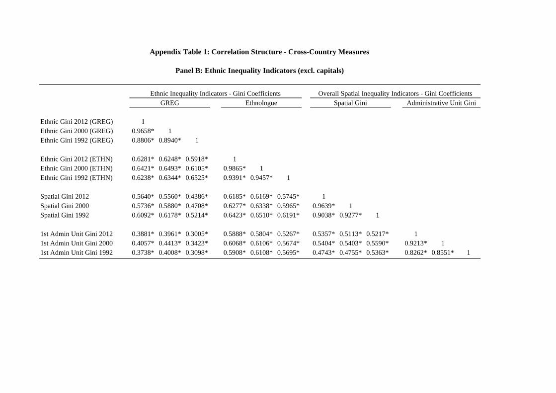
Ethnic Gini 2012 (GREG) 1Ethnic Gini 2000 (GREG) 0.9658* 1Ethnic Gini 1992 (GREG) 0.8806* 0.8940* 1
Ethnic Gini 2012 (ETHN) 0.6281* 0.6248* 0.5918* 1Ethnic Gini 2000 (ETHN) 0.6421* 0.6493* 0.6105* 0.9865* 1Ethnic Gini 1992 (ETHN) 0.6238* 0.6344* 0.6525* 0.9391* 0.9457* 1
Spatial Gini 2012 0.5640* 0.5560* 0.4386* 0.6185* 0.6169* 0.5745* 1Spatial Gini 2000 0.5736* 0.5880* 0.4708* 0.6277* 0.6338* 0.5965* 0.9639* 1Spatial Gini 1992 0.6092* 0.6178* 0.5214* 0.6423* 0.6510* 0.6191* 0.9038* 0.9277* 1
1st Admin Unit Gini 2012 0.3881* 0.3961* 0.3005* 0.5888* 0.5804* 0.5267* 0.5357* 0.5113* 0.5217* 11st Admin Unit Gini 2000 0.4057* 0.4413* 0.3423* 0.6068* 0.6106* 0.5674* 0.5404* 0.5403* 0.5590* 0.9213* 11st Admin Unit Gini 1992 0.3738* 0.4008* 0.3098* 0.5908* 0.6108* 0.5695* 0.4743* 0.4755* 0.5363* 0.8262* 0.8551* 1
Appendix Table 1: Correlation Structure - Cross-Country Measures
Panel B: Ethnic Inequality Indicators (excl. capitals)
Ethnic Inequality Indicators - Gini Coefficients Overall Spatial Inequality Indicators - Gini CoefficientsGREG Ethnologue Spatial Gini Administrative Unit Gini
Ethnic Gini 2012 (GREG) 1Ethnic Gini 2000 (GREG) 0.9586* 1Ethnic Gini 1992 (GREG) 0.9176* 0.9458* 1
Ethnic Gini 2012 (ETHN) 0.7586* 0.7394* 0.7435* 1Ethnic Gini 2000 (ETHN) 0.7509* 0.7676* 0.7659* 9663 1Ethnic Gini 1992 (ETHN) 0.7772* 0.7767* 0.8030* 93920.9578* 1
Spatial Gini 2012 0.6459* 0.6326* 0.6339* 0.7054* 0.7183* 0.688 1Spatial Gini 2000 0.6703* 0.7091* 0.6758* 0.6912* 0.7381* 0.692 0.9393* 1Spatial Gini 1992 0.7025* 0.7219* 0.7407* 0.6823* 0.7202* 0.734 0.8961* 0.9254* 1
1st Admin Unit Gini 2012 0.5633* 0.5595* 0.5580* 0.6139* 0.6182* 0.588 0.6534* 0.6273* 0.6177* 11st Admin Unit Gini 2000 0.5955* 0.6396* 0.6162* 0.6095* 0.6553* 0.610 0.6544* 0.7144* 0.6788* 0.9147* 11st Admin Unit Gini 1992 0.5805* 0.6041* 0.6335* 0.5592* 0.5871* 0.605 0.5662* 0.6000* 0.7006* 0.8505* 0.8797* 1
Ethnologue Spatial Gini Administrative Unit Gini
The table gives the correlation structure of the main ethnic inequality, overall spatial inequality and administrative unit inequality measures (Gini coefficients) in 1992, 2000, and 2012. For the construction of the ethnic and the spatial inequality measures (Gini coefficients) in Panel A we use all ethnic (linguistic) homelands and pixels/admin units; in Panel B we exclude ethnic areas, pixels and administrative units where capital cities fall; in Panel C we exclude small polygons (ethnic groups, pixels and admin units) consisting of less than one percent of a country’s population. Section 2 gives details on the construction of the ethnic inequality and spatial inequality (Gini) indexes. * indicate statistical significance at the 5% level.
Appendix Table 1: Correlation Structure - Cross-Country Measures
Panel C: Ethnic Inequality Indicators (excl. small areas)
Ethnic Inequality Indicators - Gini Coefficients Overall Spatial Inequality Indicators - Gini CoefficientsGREG
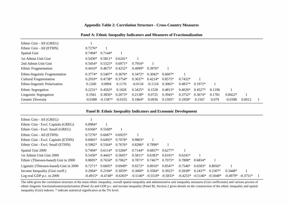
Ethnic Gini - All (GREG) 1Ethnic Gini - All (ETHN) 0.7276* 1Spatial Gini 0.7494* 0.7144* 11st Admin Unit Gini 0.5430* 0.5811* 0.6241* 12nd Admin Unit Gini 0.5454* 0.5525* 0.6971* 0.7954* 1Ethnic Fragmentation 0.4410* 0.4675* 0.4252* 0.4099* 0.3976* 1Ethno-linguistic Fragmentation 0.3774* 0.5407* 0.3676* 0.3472* 0.3042* 0.6607* 1Cultural Fragmentation 0.2910* 0.4738* 0.3754* 0.3637* 0.4214* 0.8575* 0.7432* 1Ethno-linguistic Polarization 0.1260 0.0894 0.1176 -0.0134 -0.1124 0.3065* 0.4837* 0.1972* 1Ethnic Segregation 0.2231* 0.4563* 0.1828 0.3425* 0.1528 0.4813* 0.4026* 0.4527* 0.1196 1Linguistic Segregation 0.1941 0.3856* 0.2073* 0.2138* 0.0725 0.3945* 0.3752* 0.3674* 0.1781 0.8422* 1Genetic Diversity -0.0388 -0.1587* -0.0335 0.1864* 0.0936 0.1595* 0.1858* 0.1567 0.079 -0.0398 0.0012 1
Ethnic Gini - All (GREG) 1Ethnic Gini - Excl. Capitals (GREG) 0.8984* 1Ethnic Gini - Excl. Small (GREG) 0.6566* 0.5569* 1Ethnic Gini - All (ETHN) 0.7276* 0.6687* 0.6925* 1Ethnic Gini - Excl. Capitals (ETHN) 0.6965* 0.6493* 0.7078* 0.9803* 1Ethnic Gini - Excl. Small (ETHN) 0.5982* 0.5564* 0.7676* 0.8286* 0.7890* 1Spatial Gini 2000 0.7494* 0.6114* 0.5284* 0.7144* 0.6837* 0.6277* 11st Admin Unit Gini 2000 0.5430* 0.4441* 0.5605* 0.5811* 0.6383* 0.6101* 0.6241* 1Ethnic (Thiessen-based) Gini in 2000 0.8695* 0.7634* 0.7062* 0.7871* 0.7467* 0.7075* 0.7808* 0.6834* 1Liguistic (Thiessen-based) Gini in 2000 0.7271* 0.6605* 0.6949* 0.9272* 0.8916* 0.8547* 0.7546* 0.6583* 0.8056* 1Income Inequality (Gini coeff.) 0.2064* 0.2194* 0.3059* 0.3660* 0.3584* 0.3922* 0.2838* 0.2437* 0.2307* 0.3448* 1Log real GDP p.c. in 2000 -0.4915* -0.4748* -0.6303* -0.5140* -0.5518* -0.5833* -0.4253* -0.5146* -0.5048* -0.4979* -0.3751* 1
Panel A: Ethnic Inequality Indicators and Measures of Fractionalization
Panel B: Ethnic Inequality Indicators and Economic Development
Appendix Table 2: Correlation Structure - Cross-Country Measures
The table gives the correlation structure of the main ethnic inequality, overall spatial inequality and administrative unit inequality measures (Gini coefficients) and various proxies of ethnic-lingustic fractionalization/polarization (Panel A) and GDP p.c. and income inequality (Panel B). Section 2 gives details on the construction of the ethnic inequality and spatial inequality (Gini) indexes. * indicate statistical significance at the 5% level.
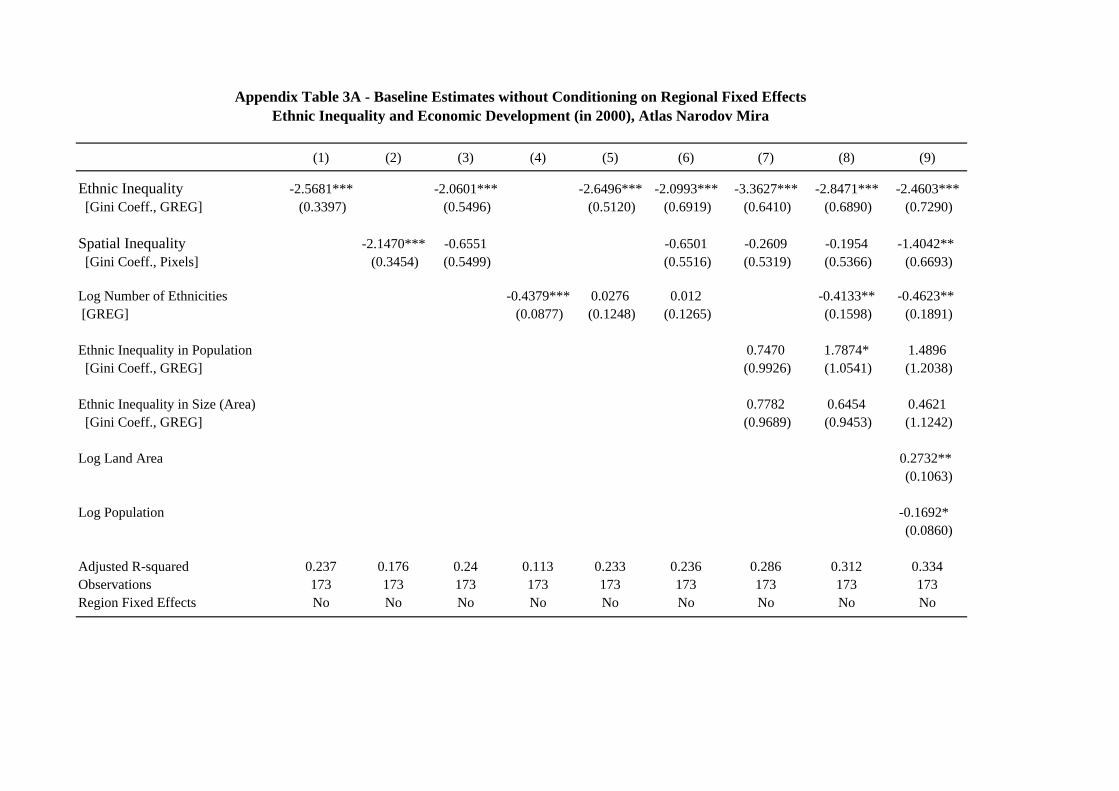
(1) (2) (3) (4) (5) (6) (7) (8) (9)
Ethnic Inequality -2.5681*** -2.0601*** -2.6496*** -2.0993*** -3.3627*** -2.8471*** -2.4603*** [Gini Coeff., GREG] (0.3397) (0.5496) (0.5120) (0.6919) (0.6410) (0.6890) (0.7290)
Spatial Inequality -2.1470*** -0.6551 -0.6501 -0.2609 -0.1954 -1.4042** [Gini Coeff., Pixels] (0.3454) (0.5499) (0.5516) (0.5319) (0.5366) (0.6693)
Log Number of Ethnicities -0.4379*** 0.0276 0.012 -0.4133** -0.4623** [GREG] (0.0877) (0.1248) (0.1265) (0.1598) (0.1891)
Ethnic Inequality in Population 0.7470 1.7874* 1.4896 [Gini Coeff., GREG] (0.9926) (1.0541) (1.2038)
Ethnic Inequality in Size (Area) 0.7782 0.6454 0.4621 [Gini Coeff., GREG] (0.9689) (0.9453) (1.1242)
Log Land Area 0.2732** (0.1063)
Log Population -0.1692* (0.0860)
Adjusted R-squared 0.237 0.176 0.24 0.113 0.233 0.236 0.286 0.312 0.334Observations 173 173 173 173 173 173 173 173 173Region Fixed Effects No No No No No No No No No
Appendix Table 3A - Baseline Estimates without Conditioning on Regional Fixed Effects Ethnic Inequality and Economic Development (in 2000), Atlas Narodov Mira
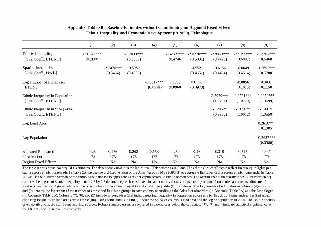
(1) (2) (3) (4) (5) (6) (7) (8) (9)
Ethnic Inequality -2.0943*** -1.7490*** -2.4589*** -2.0770*** -2.8063*** -2.5199*** -2.7707*** [Gini Coeff., ETHNO] (0.2600) (0.3663) (0.4746) (0.5891) (0.4420) (0.6007) (0.6468)
Spatial Inequality -2.1470*** -0.5989 -0.5521 -0.6136 -0.6649 -1.5692*** [Gini Coeff., Pixels] (0.3454) (0.4536) (0.4651) (0.4434) (0.4514) (0.5780)
Log Number of Languages -0.3317*** 0.0893 0.0738 -0.0856 -0.006 [ETHNO] (0.0558) (0.0960) (0.0978) (0.1075) (0.1150)
Ethnic Inequality in Population 3.2020*** 3.2731*** 2.9952*** [Gini Coeff., ETHNO] (1.0201) (1.0229) (1.0699)
Ethnic Inequality in Size (Area) -1.7462* -1.6562* -1.4419 [Gini Coeff., ETHNO] (0.9802) (1.0012) (1.0558)
Log Land Area 0.2618** (0.1005)
Log Population -0.2657*** (0.0980)
Adjusted R-squared 0.26 0.176 0.262 0.153 0.259 0.26 0.319 0.317 0.347Observations 173 173 173 173 173 173 173 173 173Region Fixed Effects No No No No No No No No No
Appendix Table 3B - Baseline Estimates without Conditioning on Regional Fixed Effects Ethnic Inequality and Economic Development (in 2000), Ethnologue
The table reports cross-country OLS estimates. The dependent variable is the log of real GDP per capita in 2000. The ethnic Gini coefficients reflect inequality in lights per capita across ethnic homelands. In Table 2A we use the digitized version of the Atlas Narodov Mira (GREG) to aggregate lights per capita across ethnic homelands. In Table 2B we use the digitized version of the Ethnologue database to aggregate lights per capita across linguistic homelands. The overall spatial inequality index (Gini coefficient) captures the degree of spatial inequality across 2.5 by 2.5 decimal degree boxes/pixels in each country (boxes intersected by national boundaries and the coastline are of smaller size). Section 2 gives details on the construction of the ethnic inequality and spatial inequality (Gini) indexes. The log number of ethnicities in columns (4)-(6), (8), and (9) denotes the logarithm of the number of ethnic and linguistic groups in each country according to the Atlas Narodov Mira (in Appendix Table 3A) and the Ethnologue (in Appendix Table 3B). Columns (7), (8), and (9) include as controls a Gini index capturing inequality in population across ethnic (linguistic) homelands and a Gini index capturing inequality in land area across ethnic (linguistic) homelands. Column (9 includes the log of country’s land area and the log of population in 2000. The Data Appendix gives detailed variable definitions and data sources. Robust standard errors are reported in parentheses below the estimates. ***, **, and * indicate statistical significance at the 1%, 5%, and 10% level, respectively.
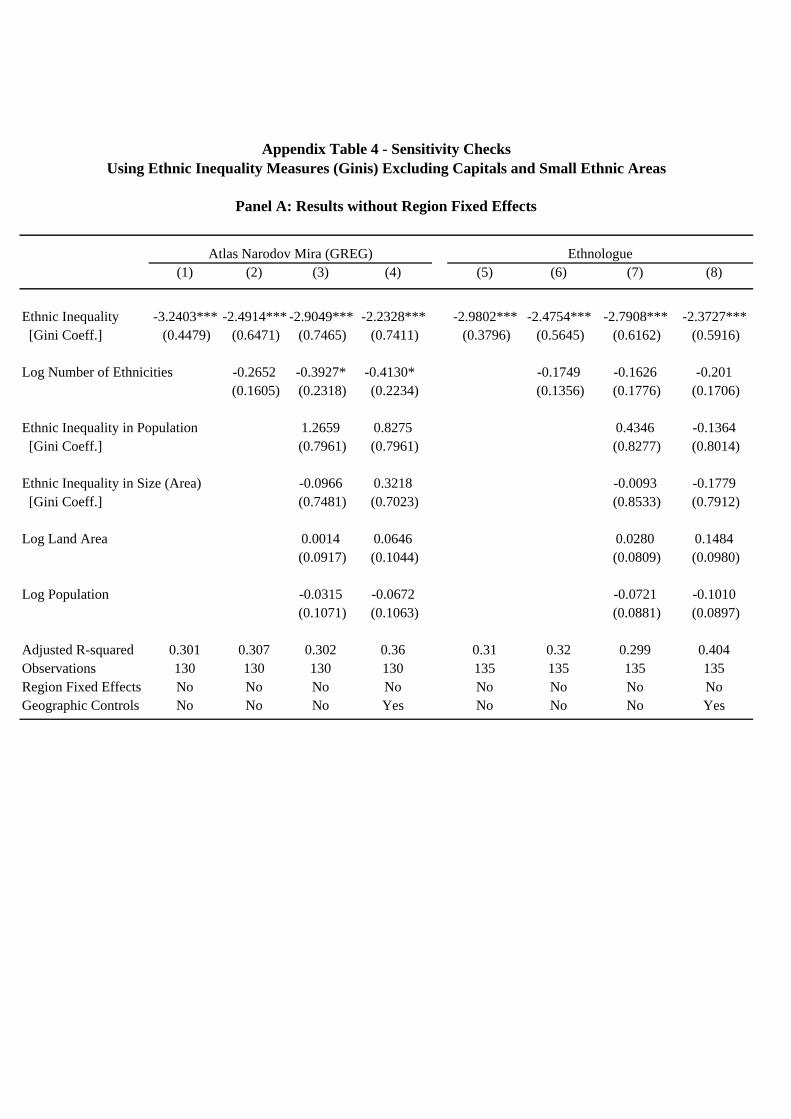
(1) (2) (3) (4) (5) (6) (7) (8)
Ethnic Inequality -3.2403*** -2.4914*** -2.9049*** -2.2328*** -2.9802*** -2.4754*** -2.7908*** -2.3727*** [Gini Coeff.] (0.4479) (0.6471) (0.7465) (0.7411) (0.3796) (0.5645) (0.6162) (0.5916)
Log Number of Ethnicities -0.2652 -0.3927* -0.4130* -0.1749 -0.1626 -0.201
(0.1605) (0.2318) (0.2234) (0.1356) (0.1776) (0.1706)
Ethnic Inequality in Population 1.2659 0.8275 0.4346 -0.1364 [Gini Coeff.] (0.7961) (0.7961) (0.8277) (0.8014)
Ethnic Inequality in Size (Area) -0.0966 0.3218 -0.0093 -0.1779 [Gini Coeff.] (0.7481) (0.7023) (0.8533) (0.7912)
Log Land Area 0.0014 0.0646 0.0280 0.1484 (0.0917) (0.1044) (0.0809) (0.0980)
Log Population -0.0315 -0.0672 -0.0721 -0.1010 (0.1071) (0.1063) (0.0881) (0.0897)
Adjusted R-squared 0.301 0.307 0.302 0.36 0.31 0.32 0.299 0.404Observations 130 130 130 130 135 135 135 135Region Fixed Effects No No No No No No No NoGeographic Controls No No No Yes No No No Yes
Appendix Table 4 - Sensitivity Checks Using Ethnic Inequality Measures (Ginis) Excluding Capitals and Small Ethnic Areas
Atlas Narodov Mira (GREG) Ethnologue
Panel A: Results without Region Fixed Effects
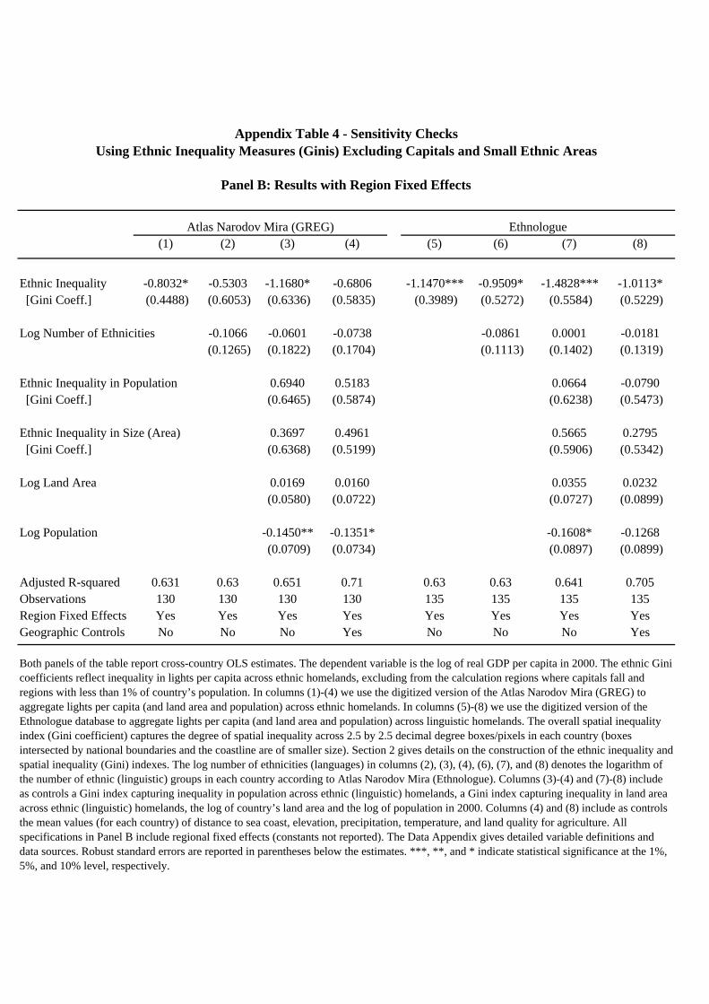
(1) (2) (3) (4) (5) (6) (7) (8)
Ethnic Inequality -0.8032* -0.5303 -1.1680* -0.6806 -1.1470*** -0.9509* -1.4828*** -1.0113* [Gini Coeff.] (0.4488) (0.6053) (0.6336) (0.5835) (0.3989) (0.5272) (0.5584) (0.5229)
Log Number of Ethnicities -0.1066 -0.0601 -0.0738 -0.0861 0.0001 -0.0181
(0.1265) (0.1822) (0.1704) (0.1113) (0.1402) (0.1319)
Ethnic Inequality in Population 0.6940 0.5183 0.0664 -0.0790 [Gini Coeff.] (0.6465) (0.5874) (0.6238) (0.5473)
Ethnic Inequality in Size (Area) 0.3697 0.4961 0.5665 0.2795 [Gini Coeff.] (0.6368) (0.5199) (0.5906) (0.5342)
Log Land Area 0.0169 0.0160 0.0355 0.0232
(0.0580) (0.0722) (0.0727) (0.0899)
Log Population -0.1450** -0.1351* -0.1608* -0.1268 (0.0709) (0.0734) (0.0897) (0.0899)
Adjusted R-squared 0.631 0.63 0.651 0.71 0.63 0.63 0.641 0.705Observations 130 130 130 130 135 135 135 135Region Fixed Effects Yes Yes Yes Yes Yes Yes Yes YesGeographic Controls No No No Yes No No No Yes
Both panels of the table report cross-country OLS estimates. The dependent variable is the log of real GDP per capita in 2000. The ethnic Gini coefficients reflect inequality in lights per capita across ethnic homelands, excluding from the calculation regions where capitals fall and regions with less than 1% of country’s population. In columns (1)-(4) we use the digitized version of the Atlas Narodov Mira (GREG) to aggregate lights per capita (and land area and population) across ethnic homelands. In columns (5)-(8) we use the digitized version of the Ethnologue database to aggregate lights per capita (and land area and population) across linguistic homelands. The overall spatial inequality index (Gini coefficient) captures the degree of spatial inequality across 2.5 by 2.5 decimal degree boxes/pixels in each country (boxes intersected by national boundaries and the coastline are of smaller size). Section 2 gives details on the construction of the ethnic inequality and spatial inequality (Gini) indexes. The log number of ethnicities (languages) in columns (2), (3), (4), (6), (7), and (8) denotes the logarithm of the number of ethnic (linguistic) groups in each country according to Atlas Narodov Mira (Ethnologue). Columns (3)-(4) and (7)-(8) include as controls a Gini index capturing inequality in population across ethnic (linguistic) homelands, a Gini index capturing inequality in land area across ethnic (linguistic) homelands, the log of country’s land area and the log of population in 2000. Columns (4) and (8) include as controls the mean values (for each country) of distance to sea coast, elevation, precipitation, temperature, and land quality for agriculture. All specifications in Panel B include regional fixed effects (constants not reported). The Data Appendix gives detailed variable definitions and data sources. Robust standard errors are reported in parentheses below the estimates. ***, **, and * indicate statistical significance at the 1%, 5%, and 10% level, respectively.
Atlas Narodov Mira (GREG) Ethnologue
Appendix Table 4 - Sensitivity Checks Using Ethnic Inequality Measures (Ginis) Excluding Capitals and Small Ethnic Areas
Panel B: Results with Region Fixed Effects
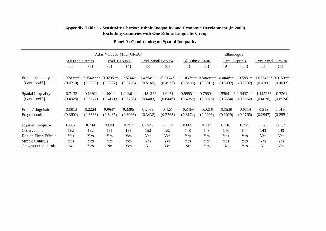
(1) (2) (3) (4) (5) (6) (7) (8) (9) (10) (11) (12)
Ethnic Inequality -1.3783*** -0.9542*** -0.9295** -0.6244* -1.4354*** -0.9174* -1.1037***-0.8049*** -0.8048** -0.5831* -1.0774***-0.9159** [Gini Coeff.] (0.4219) (0.3595) (0.3897) (0.3296) (0.5169) (0.4937) (0.3400) (0.3011) (0.3432) (0.2982) (0.4100) (0.4042)
Spatial Inequality -0.7132 -0.6392* -1.4001***-1.2436*** -1.4813** -1.0471 -0.9893** -0.7880** -1.5569***-1.3437*** -1.4952** -0.7564 [Gini Coeff.] (0.4328) (0.3777) (0.4171) (0.3733) (0.6403) (0.6446) (0.4089) (0.3976) (0.3654) (0.3662) (0.6036) (0.6524)
-0.0913 0.2224 0.0647 0.3395 0.2768 0.423 -0.3454 -0.0216 -0.3539 -0.0314 -0.318 0.0194 (0.3602) (0.3333) (0.3485) (0.3093) (0.3432) (0.3768) (0.3174) (0.2999) (0.3029) (0.2765) (0.2947) (0.2951)
adjusted R-square 0.682 0.744 0.694 0.757 0.6945 0.7428 0.689 0.737 0.710 0.755 0.692 0.734Observations 152 152 151 151 152 152 148 148 144 144 148 148Region Fixed Effects Yes Yes Yes Yes Yes Yes Yes Yes Yes Yes Yes YesSimple Controls Yes Yes Yes Yes Yes Yes Yes Yes Yes Yes Yes YesGeographic Controls No Yes No Yes No Yes No Yes No Yes No Yes
Appendix Table 5 - Sensitivity Checks : Ethnic Inequality and Economic Development (in 2000)Excluding Countries with One Ethnic-Linguistic Group
Atlas Narodov Mira (GREG) Ethnologue
Ethnic/Linguistic Fragmentation
Panel A: Conditioning on Spatial Inequality
All Ethnic Areas Excl. Capitals Excl. Small Groups All Ethnic Areas Excl. Capitals Excl. Small Groups
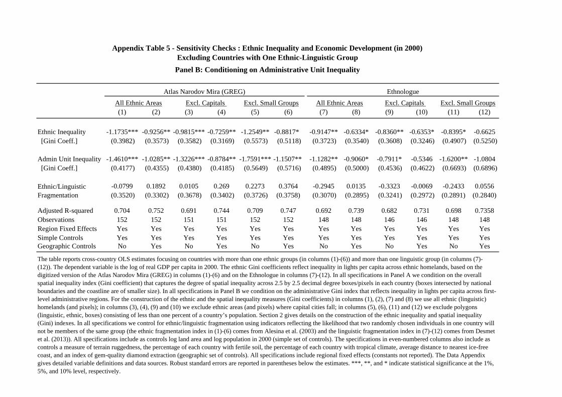
(1) (2) (3) (4) (5) (6) (7) (8) (9) (10) (11) (12)
Ethnic Inequality -1.1735*** -0.9256** -0.9815*** -0.7259** -1.2549** -0.8817* -0.9147** -0.6334* -0.8360** -0.6353* -0.8395* -0.6625 [Gini Coeff.] (0.3982) (0.3573) (0.3582) (0.3169) (0.5573) (0.5118) (0.3723) (0.3540) (0.3608) (0.3246) (0.4907) (0.5250)
Admin Unit Inequality -1.4610*** -1.0285** -1.3226*** -0.8784** -1.7591*** -1.1507** -1.1282** -0.9060* -0.7911* -0.5346 -1.6200** -1.0804 [Gini Coeff.] (0.4177) (0.4355) (0.4380) (0.4185) (0.5649) (0.5716) (0.4895) (0.5000) (0.4536) (0.4622) (0.6693) (0.6896)
-0.0799 0.1892 0.0105 0.269 0.2273 0.3764 -0.2945 0.0135 -0.3323 -0.0069 -0.2433 0.0556 (0.3520) (0.3302) (0.3678) (0.3402) (0.3726) (0.3758) (0.3070) (0.2895) (0.3241) (0.2972) (0.2891) (0.2840)
Adjusted R-squared 0.704 0.752 0.691 0.744 0.709 0.747 0.692 0.739 0.682 0.731 0.698 0.7358Observations 152 152 151 151 152 152 148 148 146 146 148 148Region Fixed Effects Yes Yes Yes Yes Yes Yes Yes Yes Yes Yes Yes YesSimple Controls Yes Yes Yes Yes Yes Yes Yes Yes Yes Yes Yes YesGeographic Controls No Yes No Yes No Yes No Yes No Yes No Yes
Appendix Table 5 - Sensitivity Checks : Ethnic Inequality and Economic Development (in 2000)Excluding Countries with One Ethnic-Linguistic Group
Ethnic/Linguistic Fragmentation
The table reports cross-country OLS estimates focusing on countries with more than one ethnic groups (in columns (1)-(6)) and more than one linguistic group (in columns (7)-(12)). The dependent variable is the log of real GDP per capita in 2000. The ethnic Gini coefficients reflect inequality in lights per capita across ethnic homelands, based on the digitized version of the Atlas Narodov Mira (GREG) in columns (1)-(6) and on the Ethnologue in columns (7)-(12). In all specifications in Panel A we condition on the overall spatial inequality index (Gini coefficient) that captures the degree of spatial inequality across 2.5 by 2.5 decimal degree boxes/pixels in each country (boxes intersected by national boundaries and the coastline are of smaller size). In all specifications in Panel B we condition on the administrative Gini index that reflects inequality in lights per capita across first-level administrative regions. For the construction of the ethnic and the spatial inequality measures (Gini coefficients) in columns (1), (2), (7) and (8) we use all ethnic (linguistic) homelands (and pixels); in columns (3), (4), (9) and (10) we exclude ethnic areas (and pixels) where capital cities fall; in columns (5), (6), (11) and (12) we exclude polygons (linguistic, ethnic, boxes) consisting of less than one percent of a country’s population. Section 2 gives details on the construction of the ethnic inequality and spatial inequality (Gini) indexes. In all specifications we control for ethnic/linguistic fragmentation using indicators reflecting the likelihood that two randomly chosen individuals in one country will not be members of the same group (the ethnic fragmentation index in (1)-(6) comes from Alesina et al. (2003) and the linguistic fragmentation index in (7)-(12) comes from Desmet et al. (2013)). All specifications include as controls log land area and log population in 2000 (simple set of controls). The specifications in even-numbered columns also include as controls a measure of terrain ruggedness, the percentage of each country with fertile soil, the percentage of each country with tropical climate, average distance to nearest ice-free coast, and an index of gem-quality diamond extraction (geographic set of controls). All specifications include regional fixed effects (constants not reported). The Data Appendix gives detailed variable definitions and data sources. Robust standard errors are reported in parentheses below the estimates. ***, **, and * indicate statistical significance at the 1%, 5%, and 10% level, respectively.
Panel B: Conditioning on Administrative Unit Inequality
Atlas Narodov Mira (GREG) EthnologueAll Ethnic Areas Excl. Capitals Excl. Small Groups All Ethnic Areas Excl. Capitals Excl. Small Groups
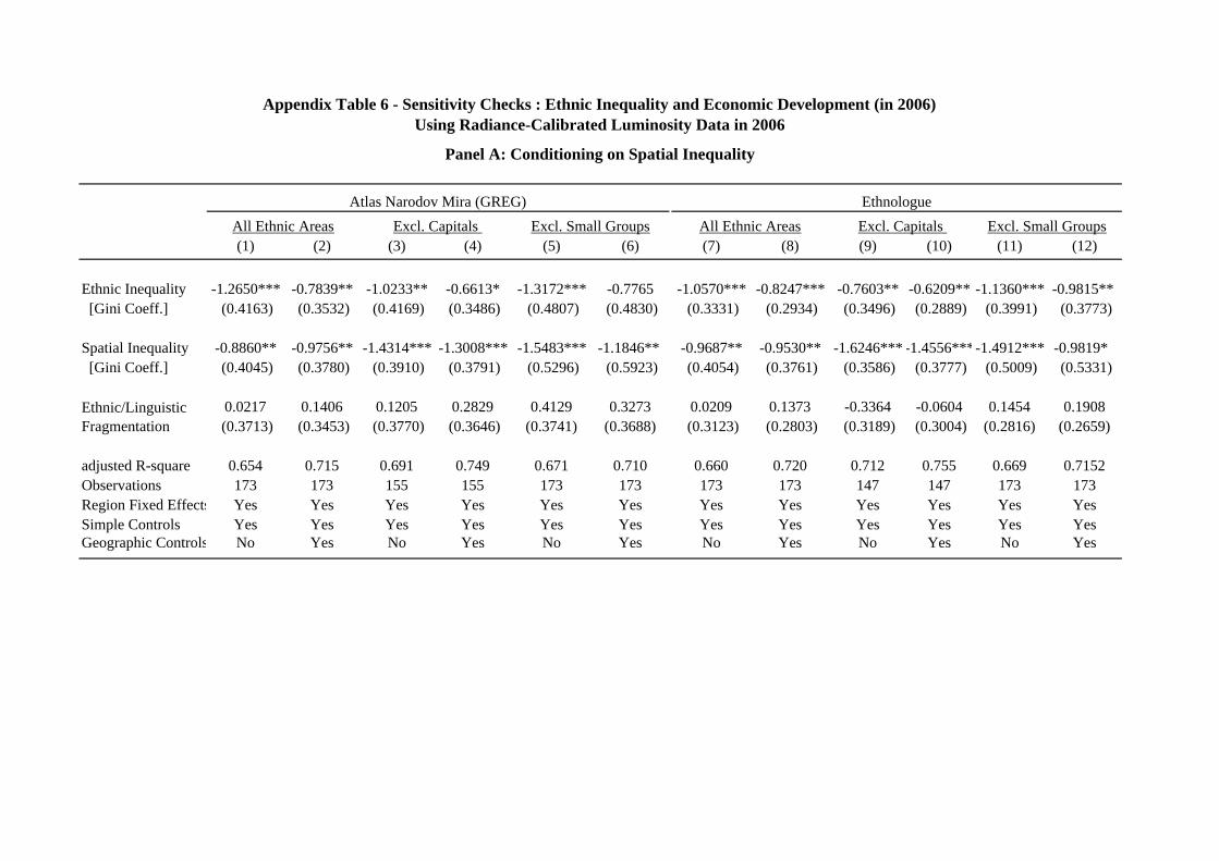
(1) (2) (3) (4) (5) (6) (7) (8) (9) (10) (11) (12)
Ethnic Inequality -1.2650*** -0.7839** -1.0233** -0.6613* -1.3172*** -0.7765 -1.0570*** -0.8247*** -0.7603** -0.6209** -1.1360*** -0.9815** [Gini Coeff.] (0.4163) (0.3532) (0.4169) (0.3486) (0.4807) (0.4830) (0.3331) (0.2934) (0.3496) (0.2889) (0.3991) (0.3773)
Spatial Inequality -0.8860** -0.9756** -1.4314*** -1.3008*** -1.5483*** -1.1846** -0.9687** -0.9530** -1.6246*** -1.4556***-1.4912*** -0.9819* [Gini Coeff.] (0.4045) (0.3780) (0.3910) (0.3791) (0.5296) (0.5923) (0.4054) (0.3761) (0.3586) (0.3777) (0.5009) (0.5331)
0.0217 0.1406 0.1205 0.2829 0.4129 0.3273 0.0209 0.1373 -0.3364 -0.0604 0.1454 0.1908 (0.3713) (0.3453) (0.3770) (0.3646) (0.3741) (0.3688) (0.3123) (0.2803) (0.3189) (0.3004) (0.2816) (0.2659)
adjusted R-square 0.654 0.715 0.691 0.749 0.671 0.710 0.660 0.720 0.712 0.755 0.669 0.7152Observations 173 173 155 155 173 173 173 173 147 147 173 173Region Fixed Effects Yes Yes Yes Yes Yes Yes Yes Yes Yes Yes Yes YesSimple Controls Yes Yes Yes Yes Yes Yes Yes Yes Yes Yes Yes YesGeographic Controls No Yes No Yes No Yes No Yes No Yes No Yes
Appendix Table 6 - Sensitivity Checks : Ethnic Inequality and Economic Development (in 2006)Using Radiance-Calibrated Luminosity Data in 2006
Panel A: Conditioning on Spatial Inequality
Atlas Narodov Mira (GREG) EthnologueAll Ethnic Areas Excl. Capitals
Ethnic/Linguistic Fragmentation
Excl. Small GroupsAll Ethnic Areas Excl. Capitals Excl. Small Groups
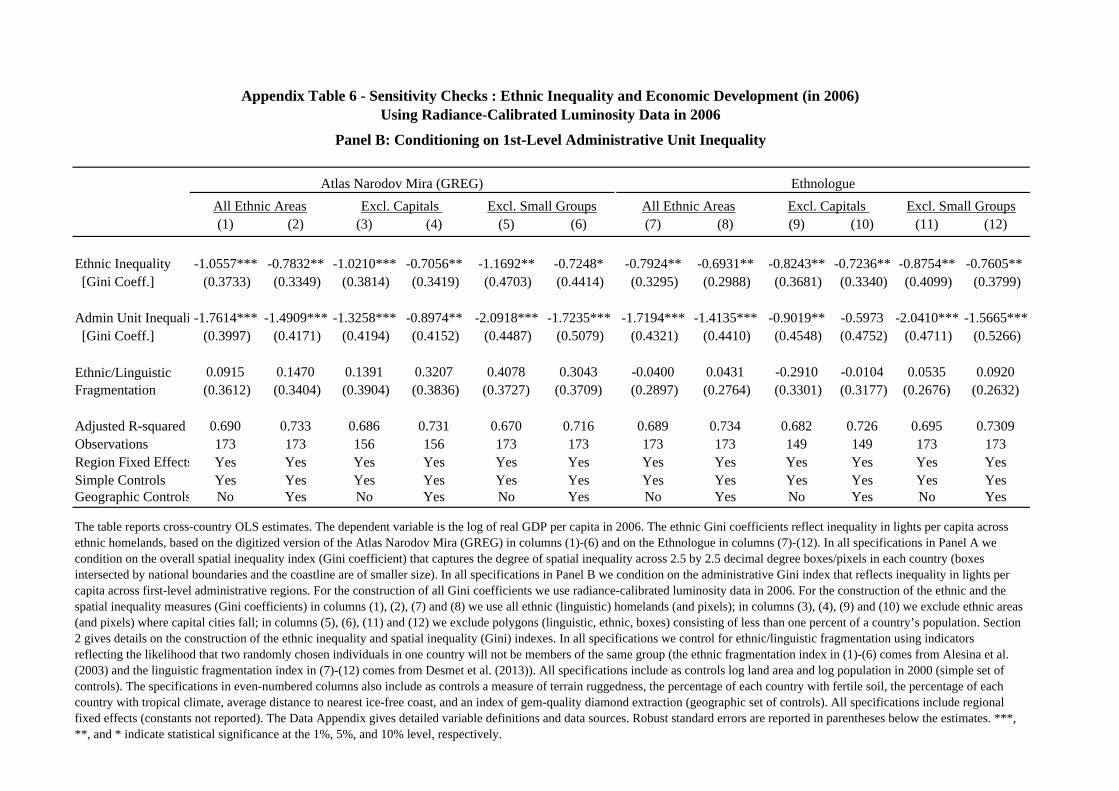
(1) (2) (3) (4) (5) (6) (7) (8) (9) (10) (11) (12)
Ethnic Inequality -1.0557*** -0.7832** -1.0210*** -0.7056** -1.1692** -0.7248* -0.7924** -0.6931** -0.8243** -0.7236** -0.8754** -0.7605** [Gini Coeff.] (0.3733) (0.3349) (0.3814) (0.3419) (0.4703) (0.4414) (0.3295) (0.2988) (0.3681) (0.3340) (0.4099) (0.3799)
Admin Unit Inequali -1.7614*** -1.4909*** -1.3258*** -0.8974** -2.0918*** -1.7235*** -1.7194*** -1.4135*** -0.9019** -0.5973 -2.0410*** -1.5665*** [Gini Coeff.] (0.3997) (0.4171) (0.4194) (0.4152) (0.4487) (0.5079) (0.4321) (0.4410) (0.4548) (0.4752) (0.4711) (0.5266)
0.0915 0.1470 0.1391 0.3207 0.4078 0.3043 -0.0400 0.0431 -0.2910 -0.0104 0.0535 0.0920 (0.3612) (0.3404) (0.3904) (0.3836) (0.3727) (0.3709) (0.2897) (0.2764) (0.3301) (0.3177) (0.2676) (0.2632)
Adjusted R-squared 0.690 0.733 0.686 0.731 0.670 0.716 0.689 0.734 0.682 0.726 0.695 0.7309Observations 173 173 156 156 173 173 173 173 149 149 173 173Region Fixed Effects Yes Yes Yes Yes Yes Yes Yes Yes Yes Yes Yes YesSimple Controls Yes Yes Yes Yes Yes Yes Yes Yes Yes Yes Yes YesGeographic Controls No Yes No Yes No Yes No Yes No Yes No Yes
Excl. Capitals Excl. Small Groups
Appendix Table 6 - Sensitivity Checks : Ethnic Inequality and Economic Development (in 2006)Using Radiance-Calibrated Luminosity Data in 2006
Panel B: Conditioning on 1st-Level Administrative Unit Inequality
Atlas Narodov Mira (GREG)
The table reports cross-country OLS estimates. The dependent variable is the log of real GDP per capita in 2006. The ethnic Gini coefficients reflect inequality in lights per capita across ethnic homelands, based on the digitized version of the Atlas Narodov Mira (GREG) in columns (1)-(6) and on the Ethnologue in columns (7)-(12). In all specifications in Panel A we condition on the overall spatial inequality index (Gini coefficient) that captures the degree of spatial inequality across 2.5 by 2.5 decimal degree boxes/pixels in each country (boxes intersected by national boundaries and the coastline are of smaller size). In all specifications in Panel B we condition on the administrative Gini index that reflects inequality in lights per capita across first-level administrative regions. For the construction of all Gini coefficients we use radiance-calibrated luminosity data in 2006. For the construction of the ethnic and the spatial inequality measures (Gini coefficients) in columns (1), (2), (7) and (8) we use all ethnic (linguistic) homelands (and pixels); in columns (3), (4), (9) and (10) we exclude ethnic areas (and pixels) where capital cities fall; in columns (5), (6), (11) and (12) we exclude polygons (linguistic, ethnic, boxes) consisting of less than one percent of a country’s population. Section 2 gives details on the construction of the ethnic inequality and spatial inequality (Gini) indexes. In all specifications we control for ethnic/linguistic fragmentation using indicators reflecting the likelihood that two randomly chosen individuals in one country will not be members of the same group (the ethnic fragmentation index in (1)-(6) comes from Alesina et al. (2003) and the linguistic fragmentation index in (7)-(12) comes from Desmet et al. (2013)). All specifications include as controls log land area and log population in 2000 (simple set of controls). The specifications in even-numbered columns also include as controls a measure of terrain ruggedness, the percentage of each country with fertile soil, the percentage of each country with tropical climate, average distance to nearest ice-free coast, and an index of gem-quality diamond extraction (geographic set of controls). All specifications include regional fixed effects (constants not reported). The Data Appendix gives detailed variable definitions and data sources. Robust standard errors are reported in parentheses below the estimates. ***, **, and * indicate statistical significance at the 1%, 5%, and 10% level, respectively.
Ethnologue
Ethnic/Linguistic Fragmentation
All Ethnic Areas Excl. Capitals Excl. Small Groups All Ethnic Areas
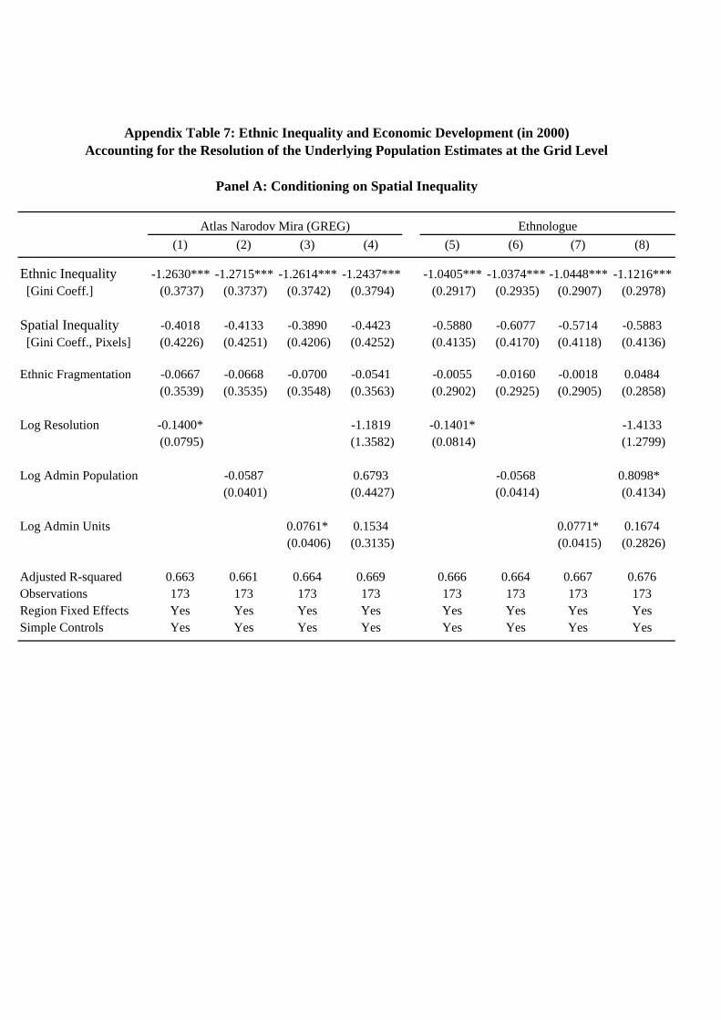
(1) (2) (3) (4) (5) (6) (7) (8)
Ethnic Inequality -1.2630*** -1.2715*** -1.2614*** -1.2437*** -1.0405*** -1.0374*** -1.0448*** -1.1216*** [Gini Coeff.] (0.3737) (0.3737) (0.3742) (0.3794) (0.2917) (0.2935) (0.2907) (0.2978)
Spatial Inequality -0.4018 -0.4133 -0.3890 -0.4423 -0.5880 -0.6077 -0.5714 -0.5883 [Gini Coeff., Pixels] (0.4226) (0.4251) (0.4206) (0.4252) (0.4135) (0.4170) (0.4118) (0.4136)
Ethnic Fragmentation -0.0667 -0.0668 -0.0700 -0.0541 -0.0055 -0.0160 -0.0018 0.0484 (0.3539) (0.3535) (0.3548) (0.3563) (0.2902) (0.2925) (0.2905) (0.2858)
Log Resolution -0.1400* -1.1819 -0.1401* -1.4133 (0.0795) (1.3582) (0.0814) (1.2799)
Log Admin Population -0.0587 0.6793 -0.0568 0.8098* (0.0401) (0.4427) (0.0414) (0.4134)
Log Admin Units 0.0761* 0.1534 0.0771* 0.1674 (0.0406) (0.3135) (0.0415) (0.2826)
Adjusted R-squared 0.663 0.661 0.664 0.669 0.666 0.664 0.667 0.676Observations 173 173 173 173 173 173 173 173Region Fixed Effects Yes Yes Yes Yes Yes Yes Yes YesSimple Controls Yes Yes Yes Yes Yes Yes Yes Yes
Appendix Table 7: Ethnic Inequality and Economic Development (in 2000)Accounting for the Resolution of the Underlying Population Estimates at the Grid Level
Panel A: Conditioning on Spatial Inequality
Atlas Narodov Mira (GREG) Ethnologue
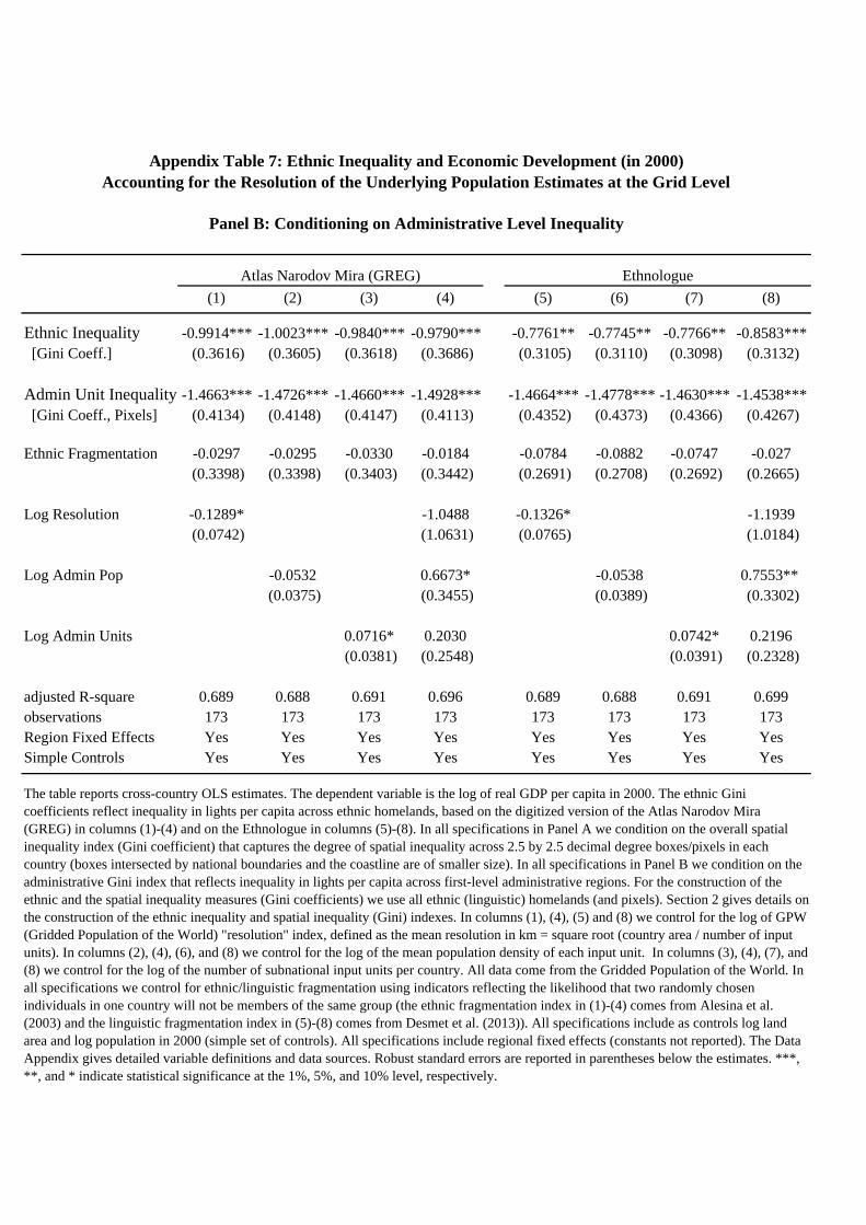
(1) (2) (3) (4) (5) (6) (7) (8)
Ethnic Inequality -0.9914*** -1.0023*** -0.9840*** -0.9790*** -0.7761** -0.7745** -0.7766** -0.8583*** [Gini Coeff.] (0.3616) (0.3605) (0.3618) (0.3686) (0.3105) (0.3110) (0.3098) (0.3132)
Admin Unit Inequality -1.4663*** -1.4726*** -1.4660*** -1.4928*** -1.4664*** -1.4778*** -1.4630*** -1.4538*** [Gini Coeff., Pixels] (0.4134) (0.4148) (0.4147) (0.4113) (0.4352) (0.4373) (0.4366) (0.4267)
Ethnic Fragmentation -0.0297 -0.0295 -0.0330 -0.0184 -0.0784 -0.0882 -0.0747 -0.027 (0.3398) (0.3398) (0.3403) (0.3442) (0.2691) (0.2708) (0.2692) (0.2665)
Log Resolution -0.1289* -1.0488 -0.1326* -1.1939 (0.0742) (1.0631) (0.0765) (1.0184)
Log Admin Pop -0.0532 0.6673* -0.0538 0.7553** (0.0375) (0.3455) (0.0389) (0.3302)
Log Admin Units 0.0716* 0.2030 0.0742* 0.2196 (0.0381) (0.2548) (0.0391) (0.2328)
adjusted R-square 0.689 0.688 0.691 0.696 0.689 0.688 0.691 0.699observations 173 173 173 173 173 173 173 173Region Fixed Effects Yes Yes Yes Yes Yes Yes Yes YesSimple Controls Yes Yes Yes Yes Yes Yes Yes Yes
The table reports cross-country OLS estimates. The dependent variable is the log of real GDP per capita in 2000. The ethnic Gini coefficients reflect inequality in lights per capita across ethnic homelands, based on the digitized version of the Atlas Narodov Mira (GREG) in columns (1)-(4) and on the Ethnologue in columns (5)-(8). In all specifications in Panel A we condition on the overall spatial inequality index (Gini coefficient) that captures the degree of spatial inequality across 2.5 by 2.5 decimal degree boxes/pixels in each country (boxes intersected by national boundaries and the coastline are of smaller size). In all specifications in Panel B we condition on the administrative Gini index that reflects inequality in lights per capita across first-level administrative regions. For the construction of the ethnic and the spatial inequality measures (Gini coefficients) we use all ethnic (linguistic) homelands (and pixels). Section 2 gives details on the construction of the ethnic inequality and spatial inequality (Gini) indexes. In columns (1), (4), (5) and (8) we control for the log of GPW (Gridded Population of the World) "resolution" index, defined as the mean resolution in km = square root (country area / number of input units). In columns (2), (4), (6), and (8) we control for the log of the mean population density of each input unit. In columns (3), (4), (7), and (8) we control for the log of the number of subnational input units per country. All data come from the Gridded Population of the World. In all specifications we control for ethnic/linguistic fragmentation using indicators reflecting the likelihood that two randomly chosen individuals in one country will not be members of the same group (the ethnic fragmentation index in (1)-(4) comes from Alesina et al. (2003) and the linguistic fragmentation index in (5)-(8) comes from Desmet et al. (2013)). All specifications include as controls log land area and log population in 2000 (simple set of controls). All specifications include regional fixed effects (constants not reported). The Data Appendix gives detailed variable definitions and data sources. Robust standard errors are reported in parentheses below the estimates. ***, **, and * indicate statistical significance at the 1%, 5%, and 10% level, respectively.
Atlas Narodov Mira (GREG) Ethnologue
Appendix Table 7: Ethnic Inequality and Economic Development (in 2000)Accounting for the Resolution of the Underlying Population Estimates at the Grid Level
Panel B: Conditioning on Administrative Level Inequality
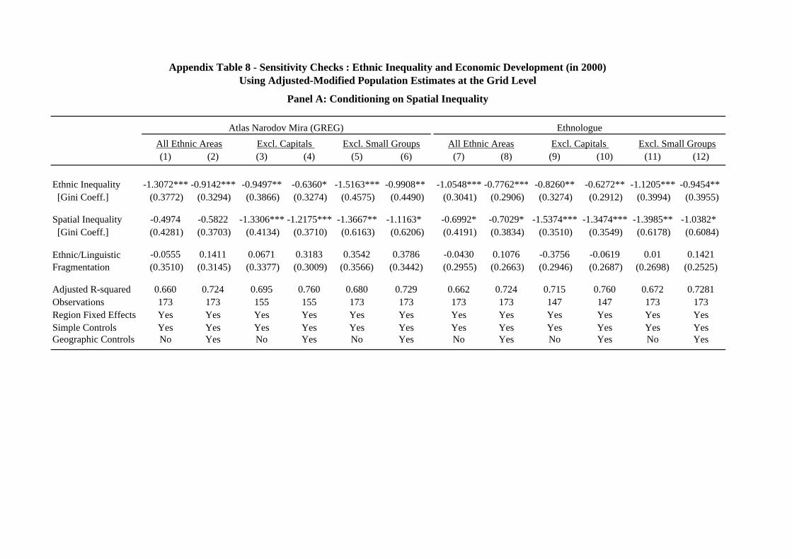
(1) (2) (3) (4) (5) (6) (7) (8) (9) (10) (11) (12)
Ethnic Inequality -1.3072*** -0.9142*** -0.9497** -0.6360* -1.5163*** -0.9908** -1.0548*** -0.7762*** -0.8260** -0.6272** -1.1205*** -0.9454** [Gini Coeff.] (0.3772) (0.3294) (0.3866) (0.3274) (0.4575) (0.4490) (0.3041) (0.2906) (0.3274) (0.2912) (0.3994) (0.3955)
Spatial Inequality -0.4974 -0.5822 -1.3306*** -1.2175*** -1.3667** -1.1163* -0.6992* -0.7029* -1.5374*** -1.3474*** -1.3985** -1.0382* [Gini Coeff.] (0.4281) (0.3703) (0.4134) (0.3710) (0.6163) (0.6206) (0.4191) (0.3834) (0.3510) (0.3549) (0.6178) (0.6084)
-0.0555 0.1411 0.0671 0.3183 0.3542 0.3786 -0.0430 0.1076 -0.3756 -0.0619 0.01 0.1421 (0.3510) (0.3145) (0.3377) (0.3009) (0.3566) (0.3442) (0.2955) (0.2663) (0.2946) (0.2687) (0.2698) (0.2525)
Adjusted R-squared 0.660 0.724 0.695 0.760 0.680 0.729 0.662 0.724 0.715 0.760 0.672 0.7281Observations 173 173 155 155 173 173 173 173 147 147 173 173Region Fixed Effects Yes Yes Yes Yes Yes Yes Yes Yes Yes Yes Yes YesSimple Controls Yes Yes Yes Yes Yes Yes Yes Yes Yes Yes Yes YesGeographic Controls No Yes No Yes No Yes No Yes No Yes No Yes
Appendix Table 8 - Sensitivity Checks : Ethnic Inequality and Economic Development (in 2000)Using Adjusted-Modified Population Estimates at the Grid Level
Panel A: Conditioning on Spatial Inequality
Atlas Narodov Mira (GREG) EthnologueAll Ethnic Areas Excl. Capitals
Ethnic/Linguistic Fragmentation
Excl. Small GroupsAll Ethnic Areas Excl. Capitals Excl. Small Groups
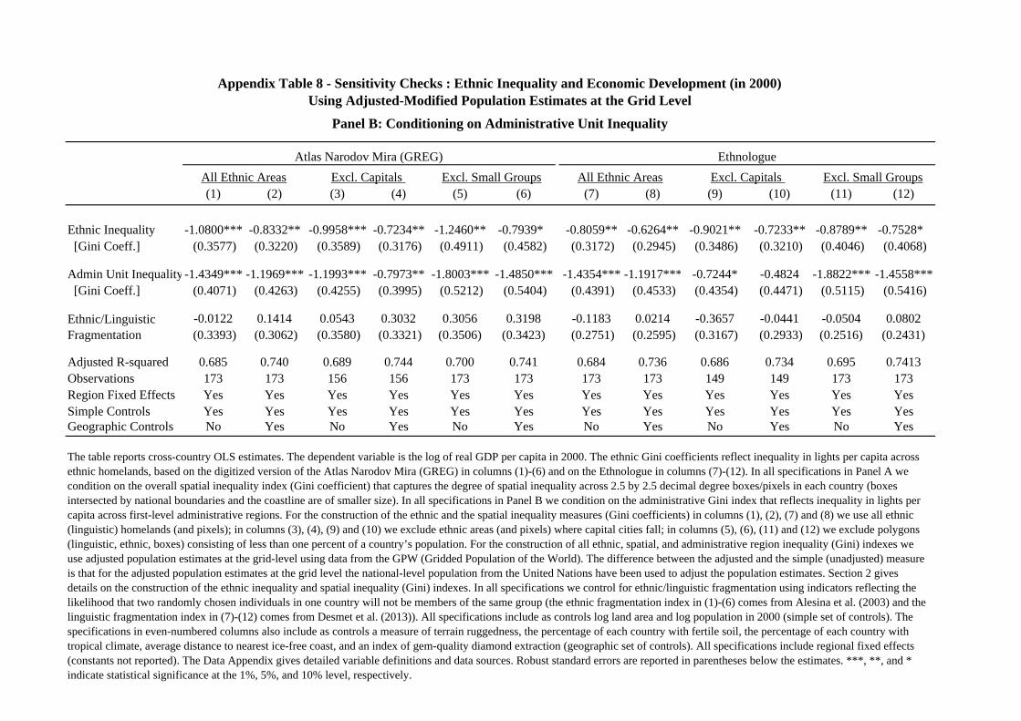
(1) (2) (3) (4) (5) (6) (7) (8) (9) (10) (11) (12)
Ethnic Inequality -1.0800*** -0.8332** -0.9958*** -0.7234** -1.2460** -0.7939* -0.8059** -0.6264** -0.9021** -0.7233** -0.8789** -0.7528* [Gini Coeff.] (0.3577) (0.3220) (0.3589) (0.3176) (0.4911) (0.4582) (0.3172) (0.2945) (0.3486) (0.3210) (0.4046) (0.4068)
Admin Unit Inequality -1.4349*** -1.1969*** -1.1993*** -0.7973** -1.8003*** -1.4850*** -1.4354*** -1.1917*** -0.7244* -0.4824 -1.8822*** -1.4558*** [Gini Coeff.] (0.4071) (0.4263) (0.4255) (0.3995) (0.5212) (0.5404) (0.4391) (0.4533) (0.4354) (0.4471) (0.5115) (0.5416)
-0.0122 0.1414 0.0543 0.3032 0.3056 0.3198 -0.1183 0.0214 -0.3657 -0.0441 -0.0504 0.0802 (0.3393) (0.3062) (0.3580) (0.3321) (0.3506) (0.3423) (0.2751) (0.2595) (0.3167) (0.2933) (0.2516) (0.2431)
Adjusted R-squared 0.685 0.740 0.689 0.744 0.700 0.741 0.684 0.736 0.686 0.734 0.695 0.7413Observations 173 173 156 156 173 173 173 173 149 149 173 173Region Fixed Effects Yes Yes Yes Yes Yes Yes Yes Yes Yes Yes Yes YesSimple Controls Yes Yes Yes Yes Yes Yes Yes Yes Yes Yes Yes YesGeographic Controls No Yes No Yes No Yes No Yes No Yes No Yes
Excl. Capitals Excl. Small Groups
Appendix Table 8 - Sensitivity Checks : Ethnic Inequality and Economic Development (in 2000)Using Adjusted-Modified Population Estimates at the Grid Level
Panel B: Conditioning on Administrative Unit Inequality
Atlas Narodov Mira (GREG)
The table reports cross-country OLS estimates. The dependent variable is the log of real GDP per capita in 2000. The ethnic Gini coefficients reflect inequality in lights per capita across ethnic homelands, based on the digitized version of the Atlas Narodov Mira (GREG) in columns (1)-(6) and on the Ethnologue in columns (7)-(12). In all specifications in Panel A we condition on the overall spatial inequality index (Gini coefficient) that captures the degree of spatial inequality across 2.5 by 2.5 decimal degree boxes/pixels in each country (boxes intersected by national boundaries and the coastline are of smaller size). In all specifications in Panel B we condition on the administrative Gini index that reflects inequality in lights per capita across first-level administrative regions. For the construction of the ethnic and the spatial inequality measures (Gini coefficients) in columns (1), (2), (7) and (8) we use all ethnic (linguistic) homelands (and pixels); in columns (3), (4), (9) and (10) we exclude ethnic areas (and pixels) where capital cities fall; in columns (5), (6), (11) and (12) we exclude polygons (linguistic, ethnic, boxes) consisting of less than one percent of a country’s population. For the construction of all ethnic, spatial, and administrative region inequality (Gini) indexes we use adjusted population estimates at the grid-level using data from the GPW (Gridded Population of the World). The difference between the adjusted and the simple (unadjusted) measure is that for the adjusted population estimates at the grid level the national-level population from the United Nations have been used to adjust the population estimates. Section 2 gives details on the construction of the ethnic inequality and spatial inequality (Gini) indexes. In all specifications we control for ethnic/linguistic fragmentation using indicators reflecting the likelihood that two randomly chosen individuals in one country will not be members of the same group (the ethnic fragmentation index in (1)-(6) comes from Alesina et al. (2003) and the linguistic fragmentation index in (7)-(12) comes from Desmet et al. (2013)). All specifications include as controls log land area and log population in 2000 (simple set of controls). The specifications in even-numbered columns also include as controls a measure of terrain ruggedness, the percentage of each country with fertile soil, the percentage of each country with tropical climate, average distance to nearest ice-free coast, and an index of gem-quality diamond extraction (geographic set of controls). All specifications include regional fixed effects (constants not reported). The Data Appendix gives detailed variable definitions and data sources. Robust standard errors are reported in parentheses below the estimates. ***, **, and * indicate statistical significance at the 1%, 5%, and 10% level, respectively.
Ethnologue
Ethnic/Linguistic Fragmentation
All Ethnic Areas Excl. Capitals Excl. Small Groups All Ethnic Areas
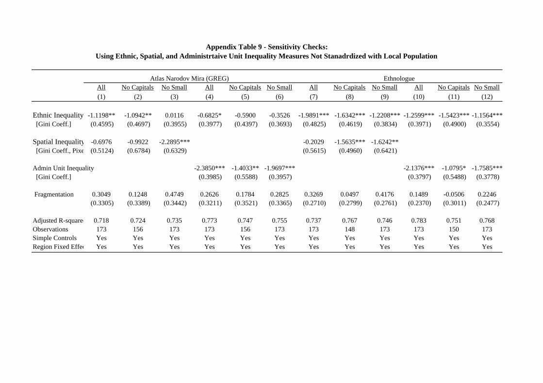
All No Capitals No Small All No Capitals No Small All No Capitals No Small All No Capitals No Small(1) (2) (3) (4) (5) (6) (7) (8) (9) (10) (11) (12)
Ethnic Inequality -1.1198** -1.0942** 0.0116 -0.6825* -0.5900 -0.3526 -1.9891*** -1.6342*** -1.2208*** -1.2599*** -1.5423*** -1.1564*** [Gini Coeff.] (0.4595) (0.4697) (0.3955) (0.3977) (0.4397) (0.3693) (0.4825) (0.4619) (0.3834) (0.3971) (0.4900) (0.3554)
Spatial Inequality -0.6976 -0.9922 -2.2895*** -0.2029 -1.5635*** -1.6242** [Gini Coeff., Pixe (0.5124) (0.6784) (0.6329) (0.5615) (0.4960) (0.6421)
Admin Unit Inequality -2.3850*** -1.4033** -1.9697*** -2.1376*** -1.0795* -1.7585*** [Gini Coeff.] (0.3985) (0.5588) (0.3957) (0.3797) (0.5488) (0.3778)
Fragmentation 0.3049 0.1248 0.4749 0.2626 0.1784 0.2825 0.3269 0.0497 0.4176 0.1489 -0.0506 0.2246
(0.3305) (0.3389) (0.3442) (0.3211) (0.3521) (0.3365) (0.2710) (0.2799) (0.2761) (0.2370) (0.3011) (0.2477)
Adjusted R-squared 0.718 0.724 0.735 0.773 0.747 0.755 0.737 0.767 0.746 0.783 0.751 0.768Observations 173 156 173 173 156 173 173 148 173 173 150 173Simple Controls Yes Yes Yes Yes Yes Yes Yes Yes Yes Yes Yes YesRegion Fixed Effec Yes Yes Yes Yes Yes Yes Yes Yes Yes Yes Yes Yes
Atlas Narodov Mira (GREG) Ethnologue
Appendix Table 9 - Sensitivity Checks: Using Ethnic, Spatial, and Administrtaive Unit Inequality Measures Not Stanadrdized with Local Population
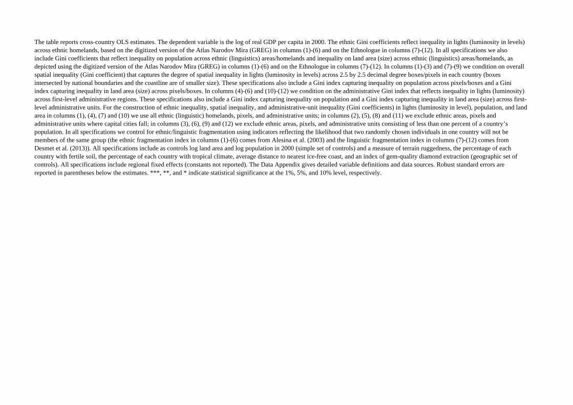
The table reports cross-country OLS estimates. The dependent variable is the log of real GDP per capita in 2000. The ethnic Gini coefficients reflect inequality in lights (luminosity in levels) across ethnic homelands, based on the digitized version of the Atlas Narodov Mira (GREG) in columns (1)-(6) and on the Ethnologue in columns (7)-(12). In all specifications we also include Gini coefficients that reflect inequality on population across ethnic (linguistics) areas/homelands and inequality on land area (size) across ethnic (linguistics) areas/homelands, as depicted using the digitized version of the Atlas Narodov Mira (GREG) in columns (1)-(6) and on the Ethnologue in columns (7)-(12). In columns (1)-(3) and (7)-(9) we condition on overall spatial inequality (Gini coefficient) that captures the degree of spatial inequality in lights (luminosity in levels) across 2.5 by 2.5 decimal degree boxes/pixels in each country (boxes intersected by national boundaries and the coastline are of smaller size). These specifications also include a Gini index capturing inequality on population across pixels/boxes and a Gini index capturing inequality in land area (size) across pixels/boxes. In columns (4)-(6) and (10)-(12) we condition on the administrative Gini index that reflects inequality in lights (luminosity) across first-level administrative regions. These specifications also include a Gini index capturing inequality on population and a Gini index capturing inequality in land area (size) across first-level administrative units. For the construction of ethnic inequality, spatial inequality, and administrative-unit inequality (Gini coefficients) in lights (luminosity in level), population, and land area in columns (1), (4), (7) and (10) we use all ethnic (linguistic) homelands, pixels, and administrative units; in columns (2), (5), (8) and (11) we exclude ethnic areas, pixels and administrative units where capital cities fall; in columns (3), (6), (9) and (12) we exclude ethnic areas, pixels, and administrative units consisting of less than one percent of a country’s population. In all specifications we control for ethnic/linguistic fragmentation using indicators reflecting the likelihood that two randomly chosen individuals in one country will not be members of the same group (the ethnic fragmentation index in columns (1)-(6) comes from Alesina et al. (2003) and the linguistic fragmentation index in columns (7)-(12) comes from Desmet et al. (2013)). All specifications include as controls log land area and log population in 2000 (simple set of controls) and a measure of terrain ruggedness, the percentage of each country with fertile soil, the percentage of each country with tropical climate, average distance to nearest ice-free coast, and an index of gem-quality diamond extraction (geographic set of controls). All specifications include regional fixed effects (constants not reported). The Data Appendix gives detailed variable definitions and data sources. Robust standard errors are reported in parentheses below the estimates. ***, **, and * indicate statistical significance at the 1%, 5%, and 10% level, respectively.
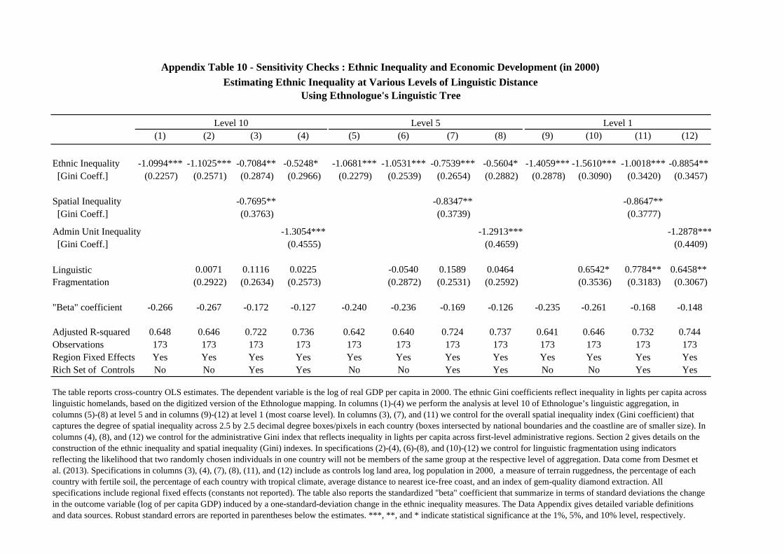
(1) (2) (3) (4) (5) (6) (7) (8) (9) (10) (11) (12)
Ethnic Inequality -1.0994*** -1.1025*** -0.7084** -0.5248* -1.0681*** -1.0531*** -0.7539*** -0.5604* -1.4059*** -1.5610*** -1.0018*** -0.8854** [Gini Coeff.] (0.2257) (0.2571) (0.2874) (0.2966) (0.2279) (0.2539) (0.2654) (0.2882) (0.2878) (0.3090) (0.3420) (0.3457)
Spatial Inequality -0.7695** -0.8347** -0.8647** [Gini Coeff.] (0.3763) (0.3739) (0.3777) Admin Unit Inequality -1.3054*** -1.2913*** -1.2878*** [Gini Coeff.] (0.4555) (0.4659) (0.4409)
0.0071 0.1116 0.0225 -0.0540 0.1589 0.0464 0.6542* 0.7784** 0.6458** (0.2922) (0.2634) (0.2573) (0.2872) (0.2531) (0.2592) (0.3536) (0.3183) (0.3067)
"Beta" coefficient -0.266 -0.267 -0.172 -0.127 -0.240 -0.236 -0.169 -0.126 -0.235 -0.261 -0.168 -0.148
Adjusted R-squared 0.648 0.646 0.722 0.736 0.642 0.640 0.724 0.737 0.641 0.646 0.732 0.744Observations 173 173 173 173 173 173 173 173 173 173 173 173Region Fixed Effects Yes Yes Yes Yes Yes Yes Yes Yes Yes Yes Yes YesRich Set of Controls No No Yes Yes No No Yes Yes No No Yes Yes
The table reports cross-country OLS estimates. The dependent variable is the log of real GDP per capita in 2000. The ethnic Gini coefficients reflect inequality in lights per capita across linguistic homelands, based on the digitized version of the Ethnologue mapping. In columns (1)-(4) we perform the analysis at level 10 of Ethnologue’s linguistic aggregation, in columns (5)-(8) at level 5 and in columns (9)-(12) at level 1 (most coarse level). In columns (3), (7), and (11) we control for the overall spatial inequality index (Gini coefficient) that captures the degree of spatial inequality across 2.5 by 2.5 decimal degree boxes/pixels in each country (boxes intersected by national boundaries and the coastline are of smaller size). In columns (4), (8), and (12) we control for the administrative Gini index that reflects inequality in lights per capita across first-level administrative regions. Section 2 gives details on the construction of the ethnic inequality and spatial inequality (Gini) indexes. In specifications (2)-(4), (6)-(8), and (10)-(12) we control for linguistic fragmentation using indicators reflecting the likelihood that two randomly chosen individuals in one country will not be members of the same group at the respective level of aggregation. Data come from Desmet et al. (2013). Specifications in columns (3), (4), (7), (8), (11), and (12) include as controls log land area, log population in 2000, a measure of terrain ruggedness, the percentage of each country with fertile soil, the percentage of each country with tropical climate, average distance to nearest ice-free coast, and an index of gem-quality diamond extraction. All specifications include regional fixed effects (constants not reported). The table also reports the standardized "beta" coefficient that summarize in terms of standard deviations the change in the outcome variable (log of per capita GDP) induced by a one-standard-deviation change in the ethnic inequality measures. The Data Appendix gives detailed variable definitions and data sources. Robust standard errors are reported in parentheses below the estimates. ***, **, and * indicate statistical significance at the 1%, 5%, and 10% level, respectively.
Appendix Table 10 - Sensitivity Checks : Ethnic Inequality and Economic Development (in 2000)Estimating Ethnic Inequality at Various Levels of Linguistic Distance
Using Ethnologue's Linguistic Tree
Linguistic Fragmentation
Level 10 Level 5 Level 1
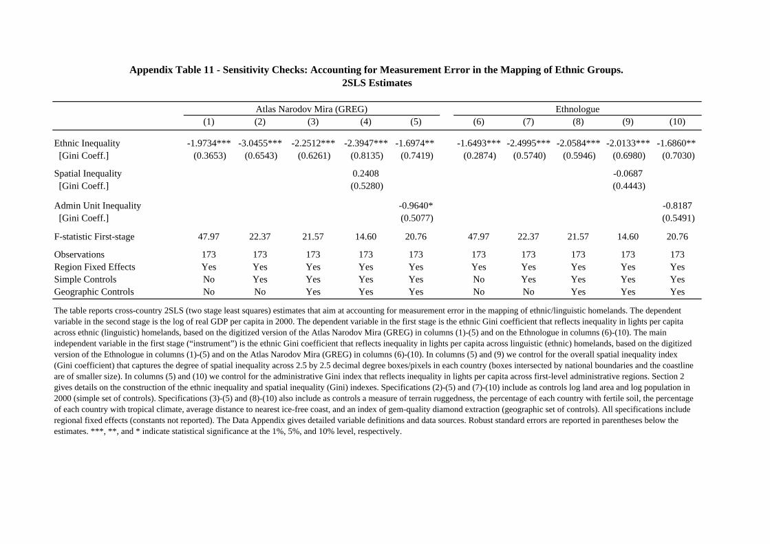
(1) (2) (3) (4) (5) (6) (7) (8) (9) (10)
Ethnic Inequality -1.9734*** -3.0455*** -2.2512*** -2.3947*** -1.6974** -1.6493*** -2.4995*** -2.0584*** -2.0133*** -1.6860** [Gini Coeff.] (0.3653) (0.6543) (0.6261) (0.8135) (0.7419) (0.2874) (0.5740) (0.5946) (0.6980) (0.7030)
Spatial Inequality 0.2408 -0.0687 [Gini Coeff.] (0.5280) (0.4443)
Admin Unit Inequality -0.9640* -0.8187 [Gini Coeff.] (0.5077) (0.5491)
F-statistic First-stage 47.97 22.37 21.57 14.60 20.76 47.97 22.37 21.57 14.60 20.76
Observations 173 173 173 173 173 173 173 173 173 173Region Fixed Effects Yes Yes Yes Yes Yes Yes Yes Yes Yes YesSimple Controls No Yes Yes Yes Yes No Yes Yes Yes YesGeographic Controls No No Yes Yes Yes No No Yes Yes Yes
Appendix Table 11 - Sensitivity Checks: Accounting for Measurement Error in the Mapping of Ethnic Groups. 2SLS Estimates
Atlas Narodov Mira (GREG) Ethnologue
The table reports cross-country 2SLS (two stage least squares) estimates that aim at accounting for measurement error in the mapping of ethnic/linguistic homelands. The dependent variable in the second stage is the log of real GDP per capita in 2000. The dependent variable in the first stage is the ethnic Gini coefficient that reflects inequality in lights per capita across ethnic (linguistic) homelands, based on the digitized version of the Atlas Narodov Mira (GREG) in columns (1)-(5) and on the Ethnologue in columns (6)-(10). The main independent variable in the first stage (“instrument”) is the ethnic Gini coefficient that reflects inequality in lights per capita across linguistic (ethnic) homelands, based on the digitized version of the Ethnologue in columns (1)-(5) and on the Atlas Narodov Mira (GREG) in columns (6)-(10). In columns (5) and (9) we control for the overall spatial inequality index (Gini coefficient) that captures the degree of spatial inequality across 2.5 by 2.5 decimal degree boxes/pixels in each country (boxes intersected by national boundaries and the coastline are of smaller size). In columns (5) and (10) we control for the administrative Gini index that reflects inequality in lights per capita across first-level administrative regions. Section 2 gives details on the construction of the ethnic inequality and spatial inequality (Gini) indexes. Specifications (2)-(5) and (7)-(10) include as controls log land area and log population in 2000 (simple set of controls). Specifications (3)-(5) and (8)-(10) also include as controls a measure of terrain ruggedness, the percentage of each country with fertile soil, the percentage of each country with tropical climate, average distance to nearest ice-free coast, and an index of gem-quality diamond extraction (geographic set of controls). All specifications include regional fixed effects (constants not reported). The Data Appendix gives detailed variable definitions and data sources. Robust standard errors are reported in parentheses below the estimates. ***, **, and * indicate statistical significance at the 1%, 5%, and 10% level, respectively.
(1) (2) (3) (4) (5) (6) (7) (8) (9) (10) (11) (12)
Ethnic Inequality -0.9352*** -0.9407***-0.9235***-0.9474*** -1.1713** -1.3893*** -0.7823***-0.8158*** -0.8994***-0.9115*** -0.9980** -1.0723** [Gini Coeff.] (0.3190) (0.3181) (0.2907) (0.2955) (0.4508) (0.4933) (0.2857) (0.2857) (0.2726) (0.2780) (0.4247) (0.4164)
Spatial Inequality -0.6993* -0.6327 -0.8560** -0.7464* -1.2744** -1.2605** -0.8591** -0.7642* -1.1543***-1.0713*** -1.1726* -1.1838* [Gini Coeff.] (0.3803) (0.4045) (0.3532) (0.3872) (0.6163) (0.6182) (0.3688) (0.3914) (0.3272) (0.3628) (0.6312) (0.6115)
0.1986 0.1768 0.3361 0.2748 0.5516* 0.5653* 0.3061 0.2842 0.1734 0.1578 0.2959 0.279 (0.3088) (0.3080) (0.3065) (0.3099) (0.3253) (0.3158) (0.2468) (0.2612) (0.2658) (0.2774) (0.2367) (0.2423)
Adjusted R-squared 0.772 0.768 0.780 0.779 0.777 0.780 0.771 0.768 0.779 0.776 0.773 0.7733Observations 151 151 143 143 151 151 151 151 135 135 151 151Region Fixed Effects Yes Yes Yes Yes Yes Yes Yes Yes Yes Yes Yes YesSimple Controls Yes Yes Yes Yes Yes Yes Yes Yes Yes Yes Yes YesGeographic Controls Yes Yes Yes Yes Yes Yes Yes Yes Yes Yes Yes YesHistorical Controls No Yes No Yes No Yes No Yes No Yes No Yes
Appendix Table 12 - Ethnic Inequality, Administrative Unit Inequality and Economic DevelopmentHistorical and Geographic Controls and Alternative Measures of Regional Inequality
Panel A: Overall Spatial Inequality
Atlas Narodov Mira (GREG) Ethnologue
Ethnic/Linguistic Fragmentation
All Ethnic Areas Excl. Capitals Excl. Small Groups All Ethnic Areas Excl. Capitals Excl. Small Groups
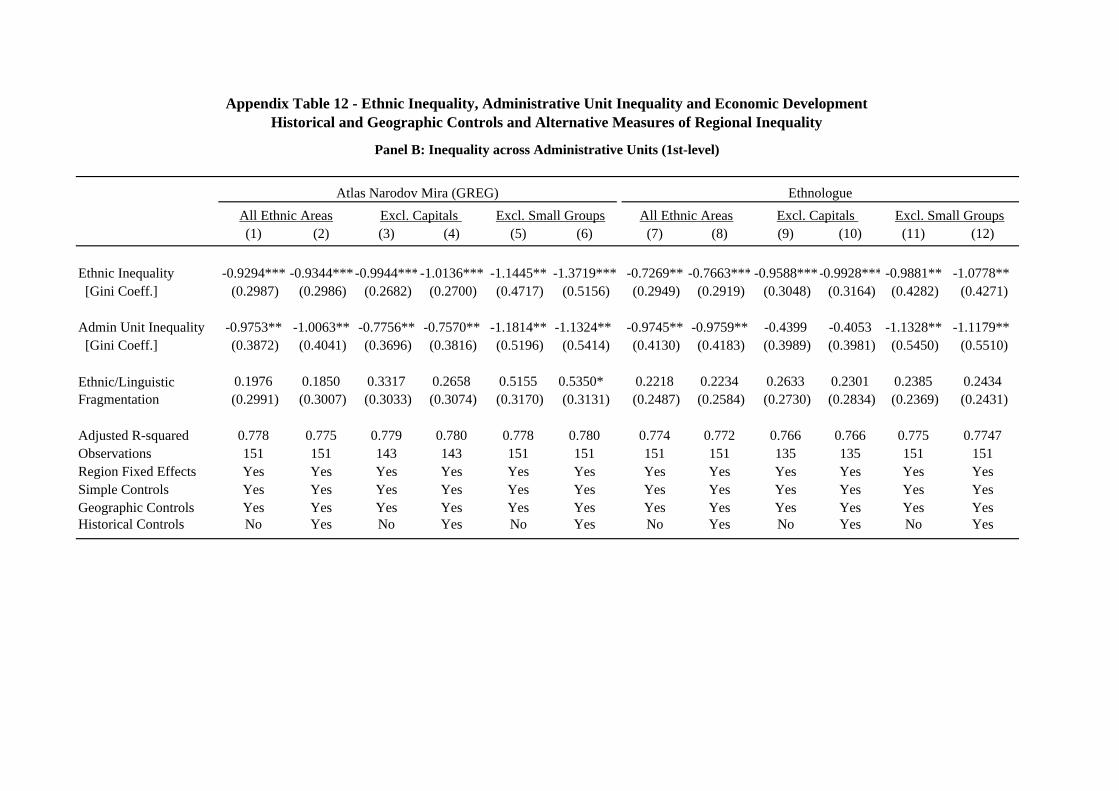
(1) (2) (3) (4) (5) (6) (7) (8) (9) (10) (11) (12)
Ethnic Inequality -0.9294*** -0.9344***-0.9944***-1.0136*** -1.1445** -1.3719*** -0.7269** -0.7663*** -0.9588***-0.9928*** -0.9881** -1.0778** [Gini Coeff.] (0.2987) (0.2986) (0.2682) (0.2700) (0.4717) (0.5156) (0.2949) (0.2919) (0.3048) (0.3164) (0.4282) (0.4271)
Admin Unit Inequality -0.9753** -1.0063** -0.7756** -0.7570** -1.1814** -1.1324** -0.9745** -0.9759** -0.4399 -0.4053 -1.1328** -1.1179** [Gini Coeff.] (0.3872) (0.4041) (0.3696) (0.3816) (0.5196) (0.5414) (0.4130) (0.4183) (0.3989) (0.3981) (0.5450) (0.5510)
0.1976 0.1850 0.3317 0.2658 0.5155 0.5350* 0.2218 0.2234 0.2633 0.2301 0.2385 0.2434 (0.2991) (0.3007) (0.3033) (0.3074) (0.3170) (0.3131) (0.2487) (0.2584) (0.2730) (0.2834) (0.2369) (0.2431)
Adjusted R-squared 0.778 0.775 0.779 0.780 0.778 0.780 0.774 0.772 0.766 0.766 0.775 0.7747Observations 151 151 143 143 151 151 151 151 135 135 151 151Region Fixed Effects Yes Yes Yes Yes Yes Yes Yes Yes Yes Yes Yes YesSimple Controls Yes Yes Yes Yes Yes Yes Yes Yes Yes Yes Yes YesGeographic Controls Yes Yes Yes Yes Yes Yes Yes Yes Yes Yes Yes YesHistorical Controls No Yes No Yes No Yes No Yes No Yes No Yes
Excl. Small Groups
Ethnic/Linguistic Fragmentation
Excl. Capitals
Panel B: Inequality across Administrative Units (1st-level)
Ethnologue
Appendix Table 12 - Ethnic Inequality, Administrative Unit Inequality and Economic DevelopmentHistorical and Geographic Controls and Alternative Measures of Regional Inequality
Atlas Narodov Mira (GREG)All Ethnic Areas Excl. Capitals Excl. Small Groups All Ethnic Areas

(1) (2) (3) (4) (5) (6) (7) (8) (9) (10) (11) (12)
Ethnic Inequality -0.9948*** -1.0401***-1.0023***-1.0162*** -1.0653** -1.3373*** -0.9125** -1.0441*** -1.0452***-1.1746***-1.0057*** -1.2415*** [Gini Coeff.] (0.3437) (0.3299) (0.2888) (0.2819) (0.4416) (0.4850) (0.3550) (0.3259) (0.3776) (0.3620) (0.3778) (0.3948)
Admin Unit Inequality -0.6844* -0.5994* -0.8006** -0.7193** -1.7258*** -1.7741*** -0.8042** -0.6894** -0.5766 -0.4735 -1.6605*** -1.6837*** [Gini Coeff.] (0.3590) (0.3510) (0.3414) (0.3308) (0.4806) (0.4565) (0.3447) (0.3214) (0.3718) (0.3527) (0.4583) (0.4318)
-0.1570 -0.2110 -0.0370 -0.1112 -0.0214 -0.0377 0.0629 0.1212 0.1157 0.1203 -0.0882 -0.0259 (0.3390) (0.3236) (0.3423) (0.3302) (0.3442) (0.3186) (0.2723) (0.2821) (0.2993) (0.3082) (0.2378) (0.2519)
Adjusted R-squared 0.789 0.795 0.793 0.798 0.807 0.822 0.789 0.797 0.780 0.785 0.808 0.8209Observations 127 127 124 124 126 126 127 127 117 117 126 126Region Fixed Effects Yes Yes Yes Yes Yes Yes Yes Yes Yes Yes Yes YesSimple Controls Yes Yes Yes Yes Yes Yes Yes Yes Yes Yes Yes YesGeographic Controls Yes Yes Yes Yes Yes Yes Yes Yes Yes Yes Yes YesHistorical Controls No Yes No Yes No Yes No Yes No Yes No Yes
Ethnic/Linguistic Fragmentation
All Ethnic Areas Excl. Capitals Excl. Small Groups All Ethnic AreasAtlas Narodov Mira (GREG) Ethnologue
Excl. Small GroupsExcl. Capitals
Appendix Table 12 - Ethnic Inequality, Administrative Unit Inequality and Economic DevelopmentHistorical and Geographic Controls and Alternative Measures of Regional Inequality
Panel C: Inequality across Administrative Units (2nd-level)
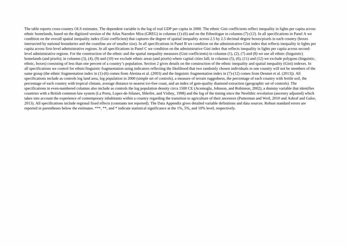
The table reports cross-country OLS estimates. The dependent variable is the log of real GDP per capita in 2000. The ethnic Gini coefficients reflect inequality in lights per capita across ethnic homelands, based on the digitized version of the Atlas Narodov Mira (GREG) in columns (1)-(6) and on the Ethnologue in columns (7)-(12). In all specifications in Panel A we condition on the overall spatial inequality index (Gini coefficient) that captures the degree of spatial inequality across 2.5 by 2.5 decimal degree boxes/pixels in each country (boxes intersected by national boundaries and the coastline are of smaller size). In all specifications in Panel B we condition on the administrative Gini index that reflects inequality in lights per capita across first-level administrative regions. In all specifications in Panel C we condition on the administrative Gini index that reflects inequality in lights per capita across second-level administrative regions. For the construction of the ethnic and the spatial inequality measures (Gini coefficients) in columns (1), (2), (7) and (8) we use all ethnic (linguistic) homelands (and pixels); in columns (3), (4), (9) and (10) we exclude ethnic areas (and pixels) where capital cities fall; in columns (5), (6), (11) and (12) we exclude polygons (linguistic, ethnic, boxes) consisting of less than one percent of a country’s population. Section 2 gives details on the construction of the ethnic inequality and spatial inequality (Gini) indexes. In all specifications we control for ethnic/linguistic fragmentation using indicators reflecting the likelihood that two randomly chosen individuals in one country will not be members of the same group (the ethnic fragmentation index in (1)-(6) comes from Alesina et al. (2003) and the linguistic fragmentation index in (7)-(12) comes from Desmet et al. (2013)). All specifications include as controls log land area, log population in 2000 (simple set of controls), a measure of terrain ruggedness, the percentage of each country with fertile soil, the percentage of each country with tropical climate, average distance to nearest ice-free coast, and an index of gem-quality diamond extraction (geographic set of controls). The specifications in even-numbered columns also include as controls the log population density circa 1500 CE (Acemoglu, Johnson, and Robinson, 2002), a dummy variable that identifies countries with a British common-law system (La Porta, Lopez-de-Silanes, Shleifer, and Vishny, 1998) and the log of the timing since the Neolithic revolution (ancestry adjusted) which takes into account the experience of contemporary inhabitants within a country regarding the transition to agriculture of their ancestors (Putterman and Weil, 2010 and Ashraf and Galor, 2013). All specifications include regional fixed effects (constants not reported). The Data Appendix gives detailed variable definitions and data sources. Robust standard errors are reported in parentheses below the estimates. ***, **, and * indicate statistical significance at the 1%, 5%, and 10% level, respectively.
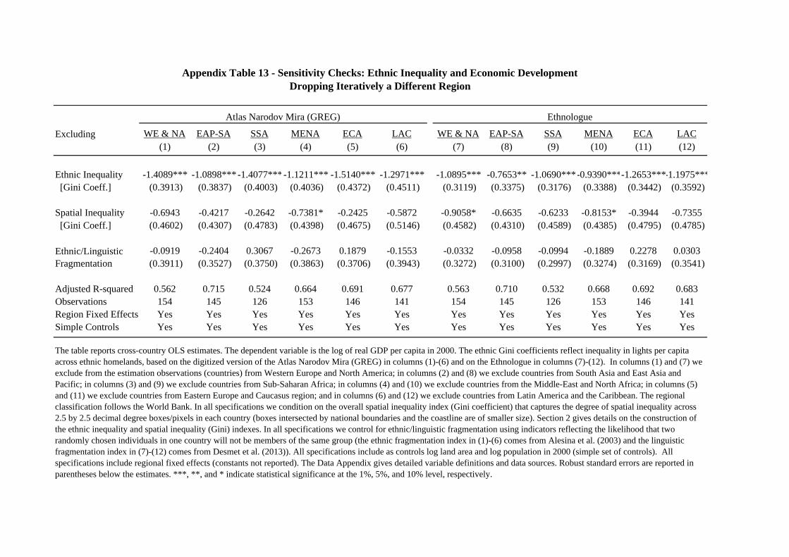
Excluding WE & NA EAP-SA SSA MENA ECA LAC WE & NA EAP-SA SSA MENA ECA LAC(1) (2) (3) (4) (5) (6) (7) (8) (9) (10) (11) (12)
Ethnic Inequality -1.4089*** -1.0898***-1.4077***-1.1211*** -1.5140*** -1.2971*** -1.0895*** -0.7653** -1.0690***-0.9390***-1.2653***-1.1975*** [Gini Coeff.] (0.3913) (0.3837) (0.4003) (0.4036) (0.4372) (0.4511) (0.3119) (0.3375) (0.3176) (0.3388) (0.3442) (0.3592)
Spatial Inequality -0.6943 -0.4217 -0.2642 -0.7381* -0.2425 -0.5872 -0.9058* -0.6635 -0.6233 -0.8153* -0.3944 -0.7355 [Gini Coeff.] (0.4602) (0.4307) (0.4783) (0.4398) (0.4675) (0.5146) (0.4582) (0.4310) (0.4589) (0.4385) (0.4795) (0.4785)
-0.0919 -0.2404 0.3067 -0.2673 0.1879 -0.1553 -0.0332 -0.0958 -0.0994 -0.1889 0.2278 0.0303 (0.3911) (0.3527) (0.3750) (0.3863) (0.3706) (0.3943) (0.3272) (0.3100) (0.2997) (0.3274) (0.3169) (0.3541)
Adjusted R-squared 0.562 0.715 0.524 0.664 0.691 0.677 0.563 0.710 0.532 0.668 0.692 0.683Observations 154 145 126 153 146 141 154 145 126 153 146 141Region Fixed Effects Yes Yes Yes Yes Yes Yes Yes Yes Yes Yes Yes YesSimple Controls Yes Yes Yes Yes Yes Yes Yes Yes Yes Yes Yes Yes
The table reports cross-country OLS estimates. The dependent variable is the log of real GDP per capita in 2000. The ethnic Gini coefficients reflect inequality in lights per capita across ethnic homelands, based on the digitized version of the Atlas Narodov Mira (GREG) in columns (1)-(6) and on the Ethnologue in columns (7)-(12). In columns (1) and (7) we exclude from the estimation observations (countries) from Western Europe and North America; in columns (2) and (8) we exclude countries from South Asia and East Asia and Pacific; in columns (3) and (9) we exclude countries from Sub-Saharan Africa; in columns (4) and (10) we exclude countries from the Middle-East and North Africa; in columns (5) and (11) we exclude countries from Eastern Europe and Caucasus region; and in columns (6) and (12) we exclude countries from Latin America and the Caribbean. The regional classification follows the World Bank. In all specifications we condition on the overall spatial inequality index (Gini coefficient) that captures the degree of spatial inequality across 2.5 by 2.5 decimal degree boxes/pixels in each country (boxes intersected by national boundaries and the coastline are of smaller size). Section 2 gives details on the construction of the ethnic inequality and spatial inequality (Gini) indexes. In all specifications we control for ethnic/linguistic fragmentation using indicators reflecting the likelihood that two randomly chosen individuals in one country will not be members of the same group (the ethnic fragmentation index in (1)-(6) comes from Alesina et al. (2003) and the linguistic fragmentation index in (7)-(12) comes from Desmet et al. (2013)). All specifications include as controls log land area and log population in 2000 (simple set of controls). All specifications include regional fixed effects (constants not reported). The Data Appendix gives detailed variable definitions and data sources. Robust standard errors are reported in parentheses below the estimates. ***, **, and * indicate statistical significance at the 1%, 5%, and 10% level, respectively.
Ethnic/Linguistic Fragmentation
Appendix Table 13 - Sensitivity Checks: Ethnic Inequality and Economic DevelopmentDropping Iteratively a Different Region
Atlas Narodov Mira (GREG) Ethnologue
Within WE & NA EA-SA SSA MENA ECA LAC WE & NA EA-SA SSA MENA ECA LAC(1) (2) (3) (4) (5) (6) (7) (8) (9) (10) (11) (12)
Ethnic Inequality 0.1689 -2.1608** -1.3374 -2.5028*** -0.6088 -1.2646** -0.4608 -2.5940** -1.5477* -1.7024** -0.8233 -0.6104 [Gini Coeff.] (0.4659) (0.8645) (0.8584) (0.6144) (0.9048) (0.5606) (0.6818) (1.1190) (0.9156) (0.7247) (0.6479) (0.4799)
Spatial Inequality 0.0397 -0.3309 0.1470 0.7791 -0.3130 0.2693 0.4371 0.1635 0.3877 -0.3925 0.1153 -0.0810 [Gini Coeff.] (0.3237) (1.4102) (0.7910) (0.8180) (0.8730) (0.5343) (0.5338) (1.0031) (1.0545) (0.5653) (0.8278) (0.4500)
0.4341 0.8465 -0.7886 0.9809 -1.7060 0.6904 0.2422 0.7342 0.2974 0.9488 -2.1738** 0.3448 (0.4816) (0.8397) (0.8293) (0.7742) (0.9956) (0.6052) (0.3036) (1.0980) (0.7772) (0.6101) (0.8642) (0.3767)
Adjusted R-squared -0.125 0.395 0.102 0.246 0.105 0.147 -0.184 0.427 0.063 0.184 0.277 0.049Observations 19 28 47 20 27 32 19 28 47 20 27 32
The table reports cross-country OLS estimates. The dependent variable is the log of real GDP per capita in 2000. The ethnic Gini coefficients reflect inequality in lights per capita across ethnic homelands, based on the digitized version of the Atlas Narodov Mira (GREG) in columns (1)-(6) and on the Ethnologue in columns (7)-(12). In columns (1) and (7) we restrict estimation to Western Europe and North America; in columns (2) and (8) we restrict estimation to South Asia and East Asia and Pacific; in columns (3) and (9) we focus on Sub-Saharan Africa; in columns (4) and (10) we look within the Middle-East and North Africa; in columns (5) and (11) we restrict estimation to Eastern Europe and Caucasus; and in columns (6) and (12) we focus on Latin America and the Caribbean. The regional classification follows the World Bank. In all specifications we condition on the overall spatial inequality index (Gini coefficient) that captures the degree of spatial inequality across 2.5 by 2.5 decimal degree boxes/pixels in each country (boxes intersected by national boundaries and the coastline are of smaller size). Section 2 gives details on the construction of the ethnic inequality and spatial inequality (Gini) indexes. In all specifications we control for ethnic/linguistic fragmentation using indicators reflecting the likelihood that two randomly chosen individuals in one country will not be members of the same group (the ethnic fragmentation index in (1)-(6) comes from Alesina et al. (2003) and the linguistic fragmentation index in (7)-(12) comes from Desmet et al. (2013)). All specifications include as controls log land area and log population in 2000 (simple set of controls). All specifications include regional fixed effects (constants not reported). The Data Appendix gives detailed variable definitions and data sources. Robust standard errors are reported in parentheses below the estimates. ***, **, and * indicate statistical significance at the 1%, 5%, and 10% level, respectively.
Appendix Table 14 - Sensitivity Checks and Heterogeneity: Ethnic Inequality and Economic Development (in 2000)Examining the Association within Regions
Atlas Narodov Mira (GREG) Ethnologue
Ethnic/Linguistic Fragmentation
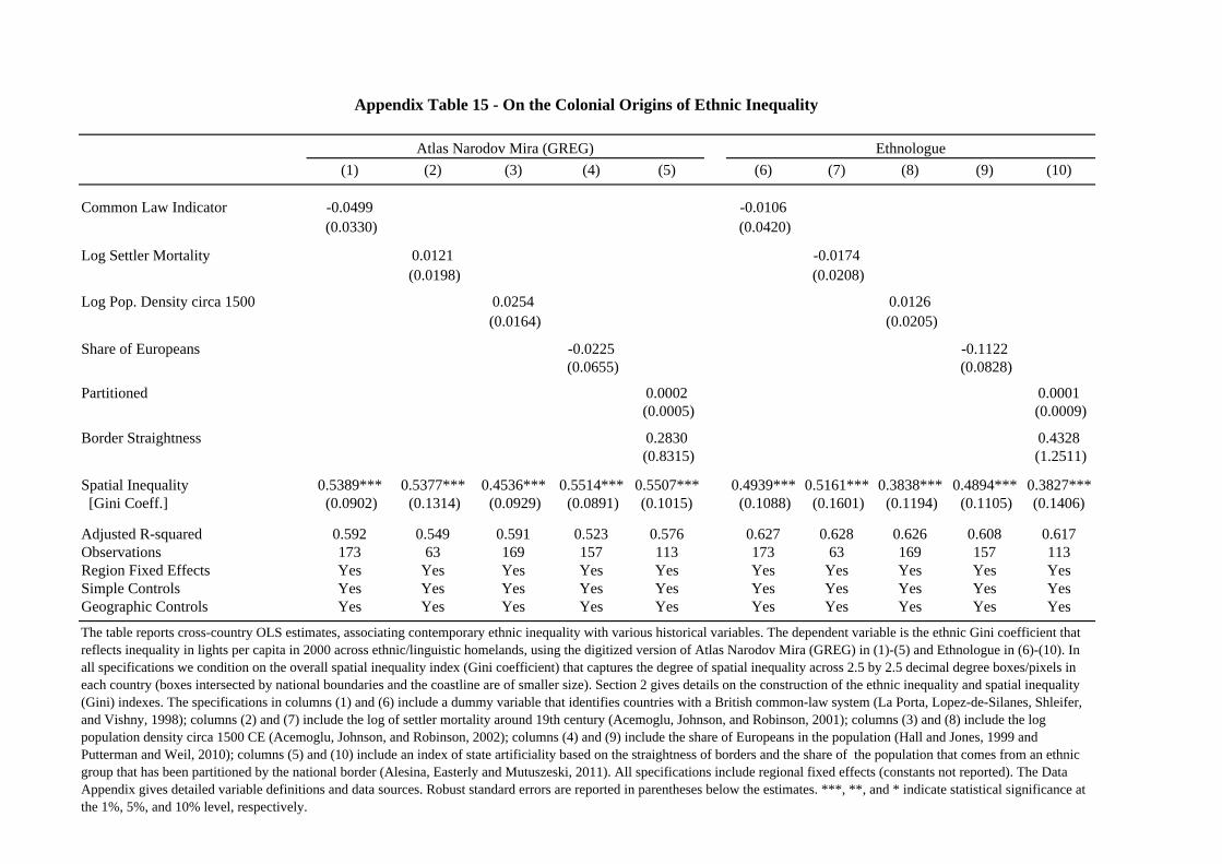
(1) (2) (3) (4) (5) (6) (7) (8) (9) (10)
Common Law Indicator -0.0499 -0.0106 (0.0330) (0.0420)
Log Settler Mortality 0.0121 -0.0174 (0.0198) (0.0208)
Log Pop. Density circa 1500 0.0254 0.0126 (0.0164) (0.0205)
Share of Europeans -0.0225 -0.1122 (0.0655) (0.0828)
Partitioned 0.0002 0.0001(0.0005) (0.0009)
Border Straightness 0.2830 0.4328(0.8315) (1.2511)
Spatial Inequality 0.5389*** 0.5377*** 0.4536*** 0.5514*** 0.5507*** 0.4939*** 0.5161*** 0.3838*** 0.4894*** 0.3827*** [Gini Coeff.] (0.0902) (0.1314) (0.0929) (0.0891) (0.1015) (0.1088) (0.1601) (0.1194) (0.1105) (0.1406)
Adjusted R-squared 0.592 0.549 0.591 0.523 0.576 0.627 0.628 0.626 0.608 0.617Observations 173 63 169 157 113 173 63 169 157 113Region Fixed Effects Yes Yes Yes Yes Yes Yes Yes Yes Yes YesSimple Controls Yes Yes Yes Yes Yes Yes Yes Yes Yes YesGeographic Controls Yes Yes Yes Yes Yes Yes Yes Yes Yes Yes
Appendix Table 15 - On the Colonial Origins of Ethnic Inequality
Atlas Narodov Mira (GREG) Ethnologue
The table reports cross-country OLS estimates, associating contemporary ethnic inequality with various historical variables. The dependent variable is the ethnic Gini coefficient that reflects inequality in lights per capita in 2000 across ethnic/linguistic homelands, using the digitized version of Atlas Narodov Mira (GREG) in (1)-(5) and Ethnologue in (6)-(10). In all specifications we condition on the overall spatial inequality index (Gini coefficient) that captures the degree of spatial inequality across 2.5 by 2.5 decimal degree boxes/pixels in each country (boxes intersected by national boundaries and the coastline are of smaller size). Section 2 gives details on the construction of the ethnic inequality and spatial inequality (Gini) indexes. The specifications in columns (1) and (6) include a dummy variable that identifies countries with a British common-law system (La Porta, Lopez-de-Silanes, Shleifer, and Vishny, 1998); columns (2) and (7) include the log of settler mortality around 19th century (Acemoglu, Johnson, and Robinson, 2001); columns (3) and (8) include the log population density circa 1500 CE (Acemoglu, Johnson, and Robinson, 2002); columns (4) and (9) include the share of Europeans in the population (Hall and Jones, 1999 and Putterman and Weil, 2010); columns (5) and (10) include an index of state artificiality based on the straightness of borders and the share of the population that comes from an ethnic group that has been partitioned by the national border (Alesina, Easterly and Mutuszeski, 2011). All specifications include regional fixed effects (constants not reported). The Data Appendix gives detailed variable definitions and data sources. Robust standard errors are reported in parentheses below the estimates. ***, **, and * indicate statistical significance at the 1%, 5%, and 10% level, respectively.
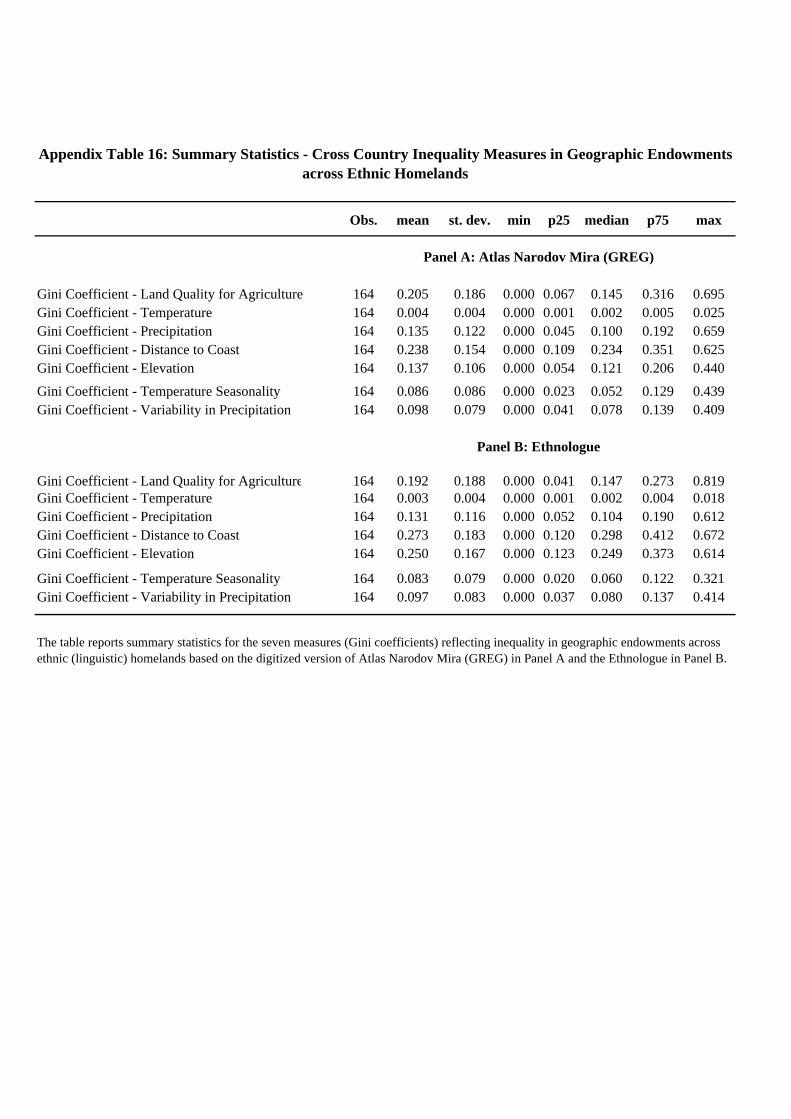
Obs. mean st. dev. min p25 median p75 max
Gini Coefficient - Land Quality for Agriculture 164 0.205 0.186 0.000 0.067 0.145 0.316 0.695Gini Coefficient - Temperature 164 0.004 0.004 0.000 0.001 0.002 0.005 0.025Gini Coefficient - Precipitation 164 0.135 0.122 0.000 0.045 0.100 0.192 0.659Gini Coefficient - Distance to Coast 164 0.238 0.154 0.000 0.109 0.234 0.351 0.625Gini Coefficient - Elevation 164 0.137 0.106 0.000 0.054 0.121 0.206 0.440
Gini Coefficient - Temperature Seasonality 164 0.086 0.086 0.000 0.023 0.052 0.129 0.439Gini Coefficient - Variability in Precipitation 164 0.098 0.079 0.000 0.041 0.078 0.139 0.409
Gini Coefficient - Land Quality for Agriculture 164 0.192 0.188 0.000 0.041 0.147 0.273 0.819Gini Coefficient - Temperature 164 0.003 0.004 0.000 0.001 0.002 0.004 0.018Gini Coefficient - Precipitation 164 0.131 0.116 0.000 0.052 0.104 0.190 0.612Gini Coefficient - Distance to Coast 164 0.273 0.183 0.000 0.120 0.298 0.412 0.672Gini Coefficient - Elevation 164 0.250 0.167 0.000 0.123 0.249 0.373 0.614
Gini Coefficient - Temperature Seasonality 164 0.083 0.079 0.000 0.020 0.060 0.122 0.321Gini Coefficient - Variability in Precipitation 164 0.097 0.083 0.000 0.037 0.080 0.137 0.414
Appendix Table 16: Summary Statistics - Cross Country Inequality Measures in Geographic Endowments across Ethnic Homelands
Panel A: Atlas Narodov Mira (GREG)
Panel B: Ethnologue
The table reports summary statistics for the seven measures (Gini coefficients) reflecting inequality in geographic endowments across ethnic (linguistic) homelands based on the digitized version of Atlas Narodov Mira (GREG) in Panel A and the Ethnologue in Panel B.
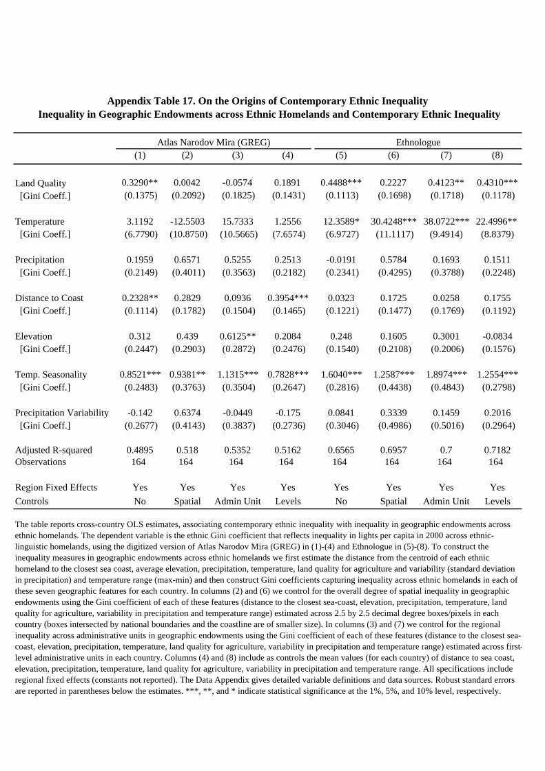
(1) (2) (3) (4) (5) (6) (7) (8)
Land Quality 0.3290** 0.0042 -0.0574 0.1891 0.4488*** 0.2227 0.4123** 0.4310*** [Gini Coeff.] (0.1375) (0.2092) (0.1825) (0.1431) (0.1113) (0.1698) (0.1718) (0.1178)
Temperature 3.1192 -12.5503 15.7333 1.2556 12.3589* 30.4248*** 38.0722*** 22.4996** [Gini Coeff.] (6.7790) (10.8750) (10.5665) (7.6574) (6.9727) (11.1117) (9.4914) (8.8379)
Precipitation 0.1959 0.6571 0.5255 0.2513 -0.0191 0.5784 0.1693 0.1511 [Gini Coeff.] (0.2149) (0.4011) (0.3563) (0.2182) (0.2341) (0.4295) (0.3788) (0.2248)
Distance to Coast 0.2328** 0.2829 0.0936 0.3954*** 0.0323 0.1725 0.0258 0.1755 [Gini Coeff.] (0.1114) (0.1782) (0.1504) (0.1465) (0.1221) (0.1477) (0.1769) (0.1192)
Elevation 0.312 0.439 0.6125** 0.2084 0.248 0.1605 0.3001 -0.0834 [Gini Coeff.] (0.2447) (0.2903) (0.2872) (0.2476) (0.1540) (0.2108) (0.2006) (0.1576)
Temp. Seasonality 0.8521*** 0.9381** 1.1315*** 0.7828*** 1.6040*** 1.2587*** 1.8974*** 1.2554*** [Gini Coeff.] (0.2483) (0.3763) (0.3504) (0.2647) (0.2816) (0.4438) (0.4843) (0.2798)
Precipitation Variability -0.142 0.6374 -0.0449 -0.175 0.0841 0.3339 0.1459 0.2016 [Gini Coeff.] (0.2677) (0.4143) (0.3837) (0.2736) (0.3046) (0.4986) (0.5016) (0.2964)
Adjusted R-squared 0.4895 0.518 0.5352 0.5162 0.6565 0.6957 0.7 0.7182Observations 164 164 164 164 164 164 164 164
Region Fixed Effects Yes Yes Yes Yes Yes Yes Yes YesControls No Spatial Admin Unit Levels No Spatial Admin Unit Levels
The table reports cross-country OLS estimates, associating contemporary ethnic inequality with inequality in geographic endowments across ethnic homelands. The dependent variable is the ethnic Gini coefficient that reflects inequality in lights per capita in 2000 across ethnic-linguistic homelands, using the digitized version of Atlas Narodov Mira (GREG) in (1)-(4) and Ethnologue in (5)-(8). To construct the inequality measures in geographic endowments across ethnic homelands we first estimate the distance from the centroid of each ethnic homeland to the closest sea coast, average elevation, precipitation, temperature, land quality for agriculture and variability (standard deviation in precipitation) and temperature range (max-min) and then construct Gini coefficients capturing inequality across ethnic homelands in each of these seven geographic features for each country. In columns (2) and (6) we control for the overall degree of spatial inequality in geographic endowments using the Gini coefficient of each of these features (distance to the closest sea-coast, elevation, precipitation, temperature, land quality for agriculture, variability in precipitation and temperature range) estimated across 2.5 by 2.5 decimal degree boxes/pixels in each country (boxes intersected by national boundaries and the coastline are of smaller size). In columns (3) and (7) we control for the regional inequality across administrative units in geographic endowments using the Gini coefficient of each of these features (distance to the closest sea-coast, elevation, precipitation, temperature, land quality for agriculture, variability in precipitation and temperature range) estimated across first-level administrative units in each country. Columns (4) and (8) include as controls the mean values (for each country) of distance to sea coast, elevation, precipitation, temperature, land quality for agriculture, variability in precipitation and temperature range. All specifications include regional fixed effects (constants not reported). The Data Appendix gives detailed variable definitions and data sources. Robust standard errors are reported in parentheses below the estimates. ***, **, and * indicate statistical significance at the 1%, 5%, and 10% level, respectively.
Appendix Table 17. On the Origins of Contemporary Ethnic Inequality Inequality in Geographic Endowments across Ethnic Homelands and Contemporary Ethnic Inequality
Atlas Narodov Mira (GREG) Ethnologue
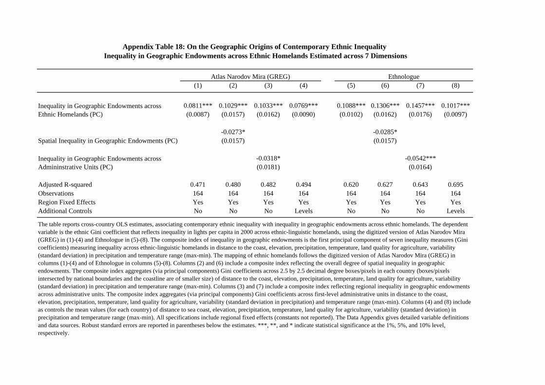
(1) (2) (3) (4) (5) (6) (7) (8)
0.0811*** 0.1029*** 0.1033*** 0.0769*** 0.1088*** 0.1306*** 0.1457*** 0.1017***(0.0087) (0.0157) (0.0162) (0.0090) (0.0102) (0.0162) (0.0176) (0.0097)
-0.0273* -0.0285*(0.0157) (0.0157)
-0.0318* -0.0542***(0.0181) (0.0164)
Adjusted R-squared 0.471 0.480 0.482 0.494 0.620 0.627 0.643 0.695Observations 164 164 164 164 164 164 164 164Region Fixed Effects Yes Yes Yes Yes Yes Yes Yes YesAdditional Controls No No No Levels No No No Levels
Spatial Inequality in Geographic Endowments (PC)
Inequality in Geographic Endowments across Admininstrative Units (PC)
The table reports cross-country OLS estimates, associating contemporary ethnic inequality with inequality in geographic endowments across ethnic homelands. The dependent variable is the ethnic Gini coefficient that reflects inequality in lights per capita in 2000 across ethnic-linguistic homelands, using the digitized version of Atlas Narodov Mira (GREG) in (1)-(4) and Ethnologue in (5)-(8). The composite index of inequality in geographic endowments is the first principal component of seven inequality measures (Gini coefficients) measuring inequality across ethnic-linguistic homelands in distance to the coast, elevation, precipitation, temperature, land quality for agriculture, variability (standard deviation) in precipitation and temperature range (max-min). The mapping of ethnic homelands follows the digitized version of Atlas Narodov Mira (GREG) in columns (1)-(4) and of Ethnologue in columns (5)-(8). Columns (2) and (6) include a composite index reflecting the overall degree of spatial inequality in geographic endowments. The composite index aggregates (via principal components) Gini coefficients across 2.5 by 2.5 decimal degree boxes/pixels in each country (boxes/pixels intersected by national boundaries and the coastline are of smaller size) of distance to the coast, elevation, precipitation, temperature, land quality for agriculture, variability (standard deviation) in precipitation and temperature range (max-min). Columns (3) and (7) include a composite index reflecting regional inequality in geographic endowments across administrative units. The composite index aggregates (via principal components) Gini coefficients across first-level administrative units in distance to the coast, elevation, precipitation, temperature, land quality for agriculture, variability (standard deviation in precipitation) and temperature range (max-min). Columns (4) and (8) include as controls the mean values (for each country) of distance to sea coast, elevation, precipitation, temperature, land quality for agriculture, variability (standard deviation) in precipitation and temperature range (max-min). All specifications include regional fixed effects (constants not reported). The Data Appendix gives detailed variable definitions and data sources. Robust standard errors are reported in parentheses below the estimates. ***, **, and * indicate statistical significance at the 1%, 5%, and 10% level, respectively.
Appendix Table 18: On the Geographic Origins of Contemporary Ethnic Inequality Inequality in Geographic Endowments across Ethnic Homelands Estimated across 7 Dimensions
Atlas Narodov Mira (GREG) Ethnologue
Inequality in Geographic Endowments across Ethnic Homelands (PC)
Inequality in Geography Estimated across (1) (2) (3) (4) (5) (6) (7) (8)
0.0538*** 0.0790*** 0.0495*** 0.0718*** 0.0880*** 0.1059*** 0.0828*** 0.0968***(0.0096) (0.0095) (0.0087) (0.0083) (0.0140) (0.0133) (0.0113) (0.0108)
Spatial Inequality in Development (Gini Coeff.) 0.4616*** 0.4463*** 0.3846*** 0.3560***(0.0632) (0.0642) (0.0784) (0.0727)
Admin Unit Inequality in Development (Gini Coeff) 0.4160*** 0.4184*** 0.4423*** 0.4557***(0.0766) (0.0755) (0.1023) (0.0944)
Adjusted R-squared 0.591 0.539 0.598 0.560 0.637 0.641 0.663 0.679Observations 164 164 164 164 164 164 164 164Region Fixed Effects Yes Yes Yes Yes Yes Yes Yes Yes
Appendix Table 19: On the Origins of Contemporary Ethnic Inequality Inequality in Geographic Endowments across Ethnic Homelands and Contemporary Ethnic Inequality
Conditional on Inequality in Development across Space and across Administrative Units
Atlas Narodov Mira (GREG) Ethnologue
The table reports cross-country OLS estimates, associating contemporary ethnic inequality in 2000 with inequality in geographic endowments across ethnic homelands, conditional on the overall degree of spatial inequality in development (in odd-numbered columns) and conditional on regional inequality across first-level administrative units (in even-numbered columns). The dependent variable is the ethnic Gini coefficient that reflects inequality in lights per capita across ethnic-linguistic homelands, using the digitized version of Atlas Narodov Mira (GREG) in (1)-(4) and Ethnologue in (5)-(8). The composite index of inequality in geographic endowments is the first principal component of five (in columns (1)-(2), (5)-(6)) or seven (in columns (3)-(4), (7)-(8)) inequality measures (Gini coefficients) measuring inequality across ethnic-linguistic homelands in distance to the coast, elevation, precipitation, temperature, and land quality for agriculture (and in columns (3)-(4) and (7)-(8) also variability (standard deviation) in precipitation and temperature range (max-min)). The mapping of ethnic homelands follows the digitized version of Atlas Narodov Mira (GREG) in columns (1)-(4) and of Ethnologue in columns (5)-(8). In odd-numbered columns we condition on the overall spatial inequality index (Gini coefficient) that captures the degree of spatial inequality across 2.5 by 2.5 decimal degree boxes/pixels in each country (boxes intersected by national boundaries and the coastline are of smaller size). In even-numbered columns we condition on the administrative Gini index that reflects inequality in lights per capita across first-level administrative regions. All specifications include regional fixed effects (constants not reported). The Data Appendix gives detailed variable definitions and data sources. Robust standard errors are reported in parentheses below the estimates. ***, **, and * indicate statistical significance at the 1%, 5%, and 10% level, respectively.
Inequality in Geographic Endowments across Ethnic Homelands (PC)
7 variables5 variables 7 variables 5 variables
(1) (2) (3) (4) (5) (6) (7) (8)
-0.1347*** -0.0908** -0.1002** -0.0993*** -0.1293*** -0.0799 -0.0862* -0.1119***(0.0383) (0.0444) (0.0398) (0.0367) (0.0432) (0.0531) (0.0456) (0.0364)
Spatial Inequality -0.5581* -0.5770* [Gini Coeff., Pixels] (0.3311) (0.3448)
Admin Unit Inequality -1.2816*** -1.2662*** [Gini Coeff.] (0.4192) (0.4322)
Adjusted R-squared 0.635 0.639 0.660 0.691 0.633 0.637 0.656 0.696Observations 164 164 164 164 164 164 164 164Region Fixed Effects Yes Yes Yes Yes Yes Yes Yes YesAdditional Controls No No No Levels No No No Levels
Appendix Table 20: Inequality in Geographic Endowments across Ethnic Homelands and Contemporary Development
Atlas Narodov Mira (GREG) Ethnologue
Conditional on Inequality in Development across Space and Administrative Units
Inequality in Geographic Endowments across Ethnic Homelands (PC)
Panel A: Inequality in Geographic Endowments across Ethnic Homelands Estimated across 5 Dimensions
(1) (2) (3) (4) (5) (6) (7) (8)
-0.1143*** -0.0735* -0.0852** -0.0754** -0.1121*** -0.0703 -0.0785** -0.0878***(0.0340) (0.0391) (0.0348) (0.0317) (0.0367) (0.0441) (0.0377) (0.0312)
Spatial Inequality -0.5753* -0.5732* [Gini Coeff., Pixels] (0.3297) (0.3371)
Admin Unit Inequality -1.2983*** -1.2779*** [Gini Coeff.] (0.4170) (0.4238)
Adjusted R-squared 0.634 0.638 0.660 0.696 0.633 0.637 0.658 0.701Observations 164 164 164 164 164 164 164 164Region Fixed Effects Yes Yes Yes Yes Yes Yes Yes YesAdditional Controls No No No Levels No No No Levels
The table reports cross-country OLS estimates, associating contemporary development in 2000 with inequality in geographic endowments across ethnic homelands. The dependent variable is the log of real GDP per capita in 2000. In Panel A the composite measures of inequality in geographic endowments is the first principal component of five inequality measures (Gini coefficients) measuring inequality across ethnic-linguistic homelands (pixels and first-level administrative units) in distance to the coast, elevation, precipitation, temperature, and land quality for agriculture. In Panel B the composite measures of inequality in geographic endowments is the first principal component of five inequality measures (Gini coefficients) measuring inequality across ethnic-linguistic homelands (pixels and first-level administrative units)in distance to the coast, elevation, precipitation, temperature, land quality for agriculture, variability (standard deviation) in precipitation and temperature range (max-min). The mapping of ethnic homelands follows the digitized version of Atlas Narodov Mira (GREG) in columns (1)-(4) and of Ethnologue in columns (5)-(8). Columns (2) and (6) include a composite index reflecting the overall degree of spatial inequality in geographic endowments. Columns (3) and (7) include a composite index reflecting regional inequality in geographic endowments across administrative units. Columns (4) and (8) include as controls the mean values (for each country) of distance to the coast, elevation, precipitation, temperature, land quality for agriculture (in Panel A and B) and variability (standard deviation) in precipitation and temperature range (max-min) in Panel B. All specifications include regional fixed effects (constants not reported). The Data Appendix gives detailed variable definitions and data sources. Robust standard errors are reported in parentheses below the estimates. ***, **, and * indicate statistical significance at the 1%, 5%, and 10% level, respectively.
Atlas Narodov Mira (GREG) Ethnologue
Inequality in Geographic Endowments across Ethnic Homelands (PC)
Panel B: Inequality in Geographic Endowments across Ethnic Homelands Estimated across 7 Dimensions
Appendix Table 20: Inequality in Geographic Endowments across Ethnic Homelands and Contemporary Development Conditional on Inequality in Development across Space and Administrative Units
(1) (2) (3) (4) (5) (6) (7) (8)
-0.1143*** -0.1784*** -0.1220* -0.0754** -0.1121*** -0.1604*** -0.1157* -0.0878***(0.0340) (0.0665) (0.0622) (0.0317) (0.0367) (0.0597) (0.0597) (0.0312)
Spatial Inequality in Geographic Endowments (PC) 0.0803 0.063(0.0743) (0.0627)
0.011 0.0054(0.0837) (0.0747)
Adjusted R-squared 0.634 0.635 0.631 0.696 0.633 0.633 0.631 0.701Observations 164 164 164 164 164 164 164 164Region Fixed Effects Yes Yes Yes Yes Yes Yes Yes YesAdditional Controls No No No Levels No No No Levels
Appendix Table 21: Inequality in Geographic Endowments across Ethnic Homelands and Contemporary Development Inequality in Geographic Endowments across Ethnic Homelands Estimated across 7 Dimensions
Atlas Narodov Mira (GREG) Ethnologue
Inequality in Geographic Endowments across Ethnic Homelands (PC)
Inequality in Geographic Endowments across Administrative Units (PC)
The table reports cross-country OLS estimates, associating contemporary development with inequality in geographic endowments across ethnic homelands. The dependent variable is the log of real GDP per capita in 2000. The composite index of inequality in geographic endowments is the first principal component of seven inequality measures (Gini coefficients) measuring inequality across ethnic/linguistic homelands in distance to the coast, elevation, precipitation, temperature, land quality for agriculture, variability (standard deviation) in precipitation and temperature range (max-min). The mapping of ethnic homelands follows the digitized version of Atlas Narodov Mira (GREG) in columns (1)-(4) and of Ethnologue in columns (5)-(8). Columns (2) and (6) include a composite index reflecting the overall degree of spatial inequality in geographic endowments. The composite index aggregates (via principal components) Gini coefficients across 2.5 by 2.5 decimal degree boxes/pixels in each country (boxes/pixels intersected by national boundaries and the coastline are of smaller size) of distance to the coast, elevation, precipitation, temperature, land quality for agriculture, variability (standard deviation) in precipitation, and temperature range (max-min). Columns (3) and (7) include a composite index reflecting regional inequality in geographic endowments across administrative units. The composite index aggregates (via principal components) Gini coefficients across first-level administrative units in distance to the coast, elevation, precipitation, temperature, land quality for agriculture, variability (standard deviation) in precipitation and temperature range (max-min). Columns (4) and (8) include as controls the mean values (for each country) of distance to sea coast, elevation, precipitation, temperature, and land quality for agriculture, variability (standard deviation) in precipitation and temperature range (max-min). All specifications include regional fixed effects (constants not reported). The Data Appendix gives detailed variable definitions and data sources. Robust standard errors are reported in parentheses below the estimates. ***, **, and * indicate statistical significance at the 1%, 5%, and 10% level, respectively.
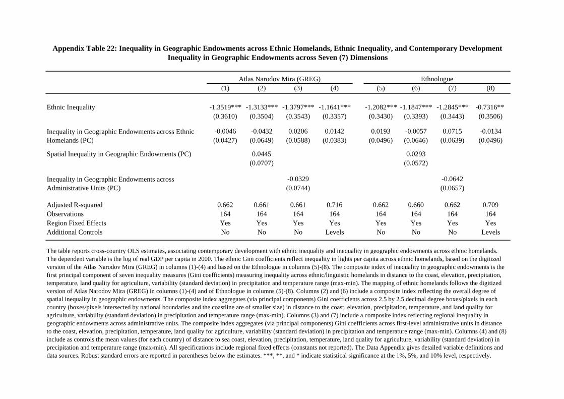
(1) (2) (3) (4) (5) (6) (7) (8)
Ethnic Inequality -1.3519*** -1.3133*** -1.3797*** -1.1641*** -1.2082*** -1.1847*** -1.2845*** -0.7316** (0.3610) (0.3504) (0.3543) (0.3357) (0.3430) (0.3393) (0.3443) (0.3506)
-0.0046 -0.0432 0.0206 0.0142 0.0193 -0.0057 0.0715 -0.0134(0.0427) (0.0649) (0.0588) (0.0383) (0.0496) (0.0646) (0.0639) (0.0496)
Spatial Inequality in Geographic Endowments (PC) 0.0445 0.0293(0.0707) (0.0572)
-0.0329 -0.0642(0.0744) (0.0657)
Adjusted R-squared 0.662 0.661 0.661 0.716 0.662 0.660 0.662 0.709Observations 164 164 164 164 164 164 164 164Region Fixed Effects Yes Yes Yes Yes Yes Yes Yes YesAdditional Controls No No No Levels No No No Levels
The table reports cross-country OLS estimates, associating contemporary development with ethnic inequality and inequality in geographic endowments across ethnic homelands. The dependent variable is the log of real GDP per capita in 2000. The ethnic Gini coefficients reflect inequality in lights per capita across ethnic homelands, based on the digitized version of the Atlas Narodov Mira (GREG) in columns (1)-(4) and based on the Ethnologue in columns (5)-(8). The composite index of inequality in geographic endowments is the first principal component of seven inequality measures (Gini coefficients) measuring inequality across ethnic/linguistic homelands in distance to the coast, elevation, precipitation, temperature, land quality for agriculture, variability (standard deviation) in precipitation and temperature range (max-min). The mapping of ethnic homelands follows the digitized version of Atlas Narodov Mira (GREG) in columns (1)-(4) and of Ethnologue in columns (5)-(8). Columns (2) and (6) include a composite index reflecting the overall degree of spatial inequality in geographic endowments. The composite index aggregates (via principal components) Gini coefficients across 2.5 by 2.5 decimal degree boxes/pixels in each country (boxes/pixels intersected by national boundaries and the coastline are of smaller size) in distance to the coast, elevation, precipitation, temperature, and land quality for agriculture, variability (standard deviation) in precipitation and temperature range (max-min). Columns (3) and (7) include a composite index reflecting regional inequality in geographic endowments across administrative units. The composite index aggregates (via principal components) Gini coefficients across first-level administrative units in distance to the coast, elevation, precipitation, temperature, land quality for agriculture, variability (standard deviation) in precipitation and temperature range (max-min). Columns (4) and (8) include as controls the mean values (for each country) of distance to sea coast, elevation, precipitation, temperature, land quality for agriculture, variability (standard deviation) in precipitation and temperature range (max-min). All specifications include regional fixed effects (constants not reported). The Data Appendix gives detailed variable definitions and data sources. Robust standard errors are reported in parentheses below the estimates. ***, **, and * indicate statistical significance at the 1%, 5%, and 10% level, respectively.
Inequality in Geographic Endowments across Administrative Units (PC)
Appendix Table 22: Inequality in Geographic Endowments across Ethnic Homelands, Ethnic Inequality, and Contemporary Development Inequality in Geographic Endowments across Seven (7) Dimensions
Atlas Narodov Mira (GREG) Ethnologue
Inequality in Geographic Endowments across Ethnic Homelands (PC)
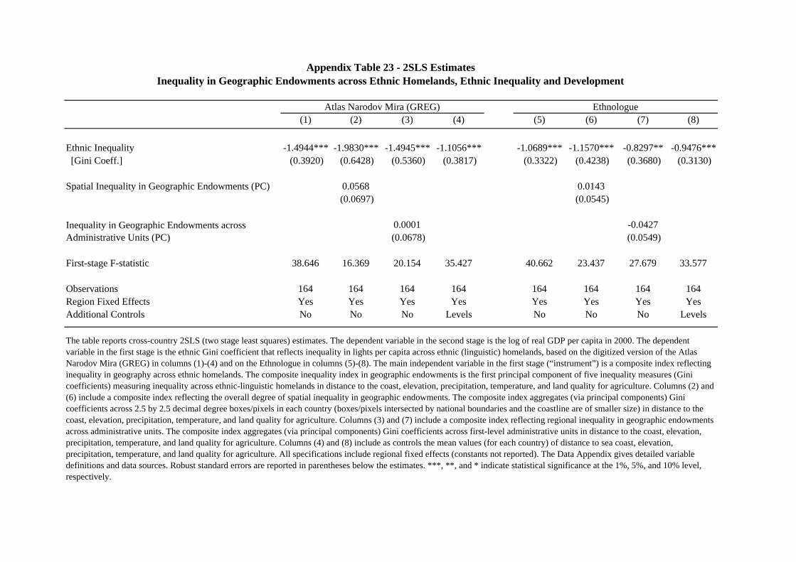
(1) (2) (3) (4) (5) (6) (7) (8)
Ethnic Inequality -1.4944*** -1.9830*** -1.4945*** -1.1056*** -1.0689*** -1.1570*** -0.8297** -0.9476*** [Gini Coeff.] (0.3920) (0.6428) (0.5360) (0.3817) (0.3322) (0.4238) (0.3680) (0.3130)
Spatial Inequality in Geographic Endowments (PC) 0.0568 0.0143 (0.0697) (0.0545)
0.0001 -0.0427 (0.0678) (0.0549)
First-stage F-statistic 38.646 16.369 20.154 35.427 40.662 23.437 27.679 33.577
Observations 164 164 164 164 164 164 164 164Region Fixed Effects Yes Yes Yes Yes Yes Yes Yes YesAdditional Controls No No No Levels No No No Levels
The table reports cross-country 2SLS (two stage least squares) estimates. The dependent variable in the second stage is the log of real GDP per capita in 2000. The dependent variable in the first stage is the ethnic Gini coefficient that reflects inequality in lights per capita across ethnic (linguistic) homelands, based on the digitized version of the Atlas Narodov Mira (GREG) in columns (1)-(4) and on the Ethnologue in columns (5)-(8). The main independent variable in the first stage (“instrument”) is a composite index reflecting inequality in geography across ethnic homelands. The composite inequality index in geographic endowments is the first principal component of five inequality measures (Gini coefficients) measuring inequality across ethnic-linguistic homelands in distance to the coast, elevation, precipitation, temperature, and land quality for agriculture. Columns (2) and (6) include a composite index reflecting the overall degree of spatial inequality in geographic endowments. The composite index aggregates (via principal components) Gini coefficients across 2.5 by 2.5 decimal degree boxes/pixels in each country (boxes/pixels intersected by national boundaries and the coastline are of smaller size) in distance to the coast, elevation, precipitation, temperature, and land quality for agriculture. Columns (3) and (7) include a composite index reflecting regional inequality in geographic endowments across administrative units. The composite index aggregates (via principal components) Gini coefficients across first-level administrative units in distance to the coast, elevation, precipitation, temperature, and land quality for agriculture. Columns (4) and (8) include as controls the mean values (for each country) of distance to sea coast, elevation, precipitation, temperature, and land quality for agriculture. All specifications include regional fixed effects (constants not reported). The Data Appendix gives detailed variable definitions and data sources. Robust standard errors are reported in parentheses below the estimates. ***, **, and * indicate statistical significance at the 1%, 5%, and 10% level, respectively.
Appendix Table 23 - 2SLS EstimatesInequality in Geographic Endowments across Ethnic Homelands, Ethnic Inequality and Development
Inequality in Geographic Endowments across Administrative Units (PC)
Atlas Narodov Mira (GREG) Ethnologue
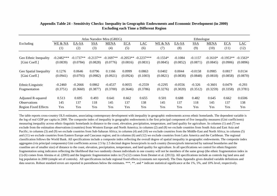
Excluding WE & NA EA-SA SSA MENA ECA LAC WE & NA EA-SA SSA MENA ECA LAC(1) (2) (3) (4) (5) (6) (7) (8) (9) (10) (11) (12)
Geo Ethnic Inequality -0.2482*** -0.1737** -0.2137** -0.1697** -0.2053** -0.2237*** -0.1554* -0.1084 -0.1157 -0.1610* -0.1953** -0.1563* [Gini Coeff.] (0.0839) (0.0784) (0.0828) (0.0776) (0.0816) (0.0831) (0.0845) (0.0852) (0.0871) (0.0845) (0.0906) (0.0896)
Geo Spatial Inequality 0.1276 0.0646 0.0796 0.1166 0.0999 0.0863 0.0402 0.0044 -0.0158 0.0985 0.0817 0.0134 [Gini Coeff.] (0.0941) (0.0793) (0.0982) (0.0921) (0.0924) (0.1003) (0.0821) (0.0838) (0.0848) (0.0818) (0.0858) (0.0870)
-0.2460 -0.2666 0.0862 -0.4537 0.0055 -0.2559 -0.2295 -0.0556 -0.326 -0.3601 0.0479 -0.293 (0.3751) (0.3660) (0.3877) (0.3700) (0.3646) (0.3786) (0.3276) (0.3020) (0.3512) (0.3259) (0.3358) (0.3781)
Adjusted R-squared 0.513 0.695 0.493 0.641 0.662 0.655 0.501 0.688 0.482 0.645 0.662 0.6506Observations 145 137 118 145 137 138 145 137 118 145 137 138Region Fixed Effects Yes Yes Yes Yes Yes Yes Yes Yes Yes Yes Yes Yes
Ethnic/Linguistic Fragmentation
The table reports cross-country OLS estimates, associating contemporary development with inequality in geographic endowments across ethnic homelands. The dependent variable is the log of real GDP per capita in 2000. The composite index of inequality in geographic endowments is the first principal component of five inequality measures (Gini coefficients) measuring inequality across ethnic-linguistic homelands in distance to the coast, elevation, precipitation, temperature, and land quality for agriculture. In columns (1) and (7) we exclude from the estimation observations (countries) from Western Europe and North America; in columns (2) and (8) we exclude countries from South Asia and East Asia and Pacific; in columns (3) and (9) we exclude countries from Sub-Saharan Africa; in columns (4) and (10) we exclude countries from the Middle-East and North Africa; in columns (5) and (11) we exclude countries from Eastern Europe and Caucasus region; and in columns (6) and (12) we exclude countries from Latin America and the Caribbean. The regional classification follows the World Bank. All specifications include a composite index reflecting the overall degree of spatial inequality in geographic endowments. The composite index aggregates (via principal components) Gini coefficients across 2.5 by 2.5 decimal degree boxes/pixels in each country (boxes/pixels intersected by national boundaries and the coastline are of smaller size) of distance to the coast, elevation, precipitation, temperature, and land quality for agriculture. In all specifications we control for ethnic/linguistic fragmentation using indicators reflecting the likelihood that two randomly chosen individuals in one country will not be members of the same group (the ethnic fragmentation index in (1)-(6) comes from Alesina et al. (2003) and the linguistic fragmentation index in (7)-(12) comes from Desmet et al. (2013)). All specifications include as controls log land area and log population in 2000 (simple set of controls). All specifications include regional fixed effects (constants not reported). The Data Appendix gives detailed variable definitions and data sources. Robust standard errors are reported in parentheses below the estimates. ***, **, and * indicate statistical significance at the 1%, 5%, and 10% level, respectively.
Appendix Table 24 - Sensitivity Checks: Inequality in Geographic Endowments and Economic Development (in 2000)Excluding each Time a Different Region
Atlas Narodov Mira (GREG) Ethnologue
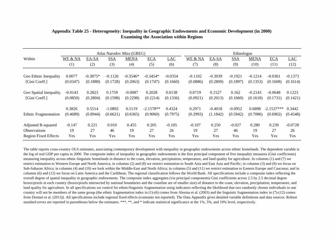
Within WE & NA EA-SA SSA MENA ECA LAC WE & NA EA-SA SSA MENA ECA LAC(1) (2) (3) (4) (5) (6) (7) (8) (9) (10) (11) (12)
Geo Ethnic Inequality 0.0077 -0.3875* -0.1126 -0.3546* -0.3454* -0.0354 -0.1102 -0.3039 -0.1921 -0.1214 -0.0361 -0.1373 [Gini Coeff.] (0.0347) (0.1888) (0.1728) (0.2063) (0.1747) (0.1660) (0.0886) (0.2809) (0.1897) (0.1353) (0.1608) (0.1614)
Geo Spatial Inequality -0.0143 0.2823 0.1759 -0.0087 0.2028 0.0138 0.0719 0.1527 0.162 -0.2143 -0.0648 0.1223 [Gini Coeff.] (0.0850) (0.2804) (0.1598) (0.2298) (0.2214) (0.1336) (0.0921) (0.2013) (0.1660) (0.1618) (0.1731) (0.1421)
0.3826 0.5514 -1.0892 0.5119 -2.1578** 0.4324 0.2971 -0.4018 -0.0952 0.6898 -2.1537*** 0.3442 (0.4689) (0.8944) (0.6621) (0.6365) (0.9060) (0.7975) (0.2993) (1.1842) (0.5942) (0.7086) (0.6902) (0.4548)
Adjusted R-squared -0.147 0.221 0.010 0.455 0.205 -0.105 -0.107 0.250 -0.027 0.280 0.239 -0.0728Observations 19 27 46 19 27 26 19 27 46 19 27 26Region Fixed Effects Yes Yes Yes Yes Yes Yes Yes Yes Yes Yes Yes Yes
Ethnic Fragmentation
The table reports cross-country OLS estimates, associating contemporary development with inequality in geographic endowments across ethnic homelands. The dependent variable is the log of real GDP per capita in 2000. The composite index of inequality in geographic endowments is the first principal component of five inequality measures (Gini coefficients) measuring inequality across ethnic-linguistic homelands in distance to the coast, elevation, precipitation, temperature, and land quality for agriculture. In columns (1) and (7) we restrict estimation to Western Europe and North America; in columns (2) and (8) we restrict estimation to South Asia and East Asia and Pacific; in columns (3) and (9) we focus on Sub-Saharan Africa; in columns (4) and (10) we look within the Middle-East and North Africa; in columns (5) and (11) we restrict estimation to Eastern Europe and Caucasus; and in columns (6) and (12) we focus on Latin America and the Caribbean. The regional classification follows the World Bank. All specifications include a composite index reflecting the overall degree of spatial inequality in geographic endowments. The composite index aggregates (via principal components) Gini coefficients across 2.5 by 2.5 decimal degree boxes/pixels in each country (boxes/pixels intersected by national boundaries and the coastline are of smaller size) of distance to the coast, elevation, precipitation, temperature, and land quality for agriculture. In all specifications we control for ethnic/linguistic fragmentation using indicators reflecting the likelihood that two randomly chosen individuals in one country will not be members of the same group (the ethnic fragmentation index in (1)-(6) comes from Alesina et al. (2003) and the linguistic fragmentation index in (7)-(12) comes from Desmet et al. (2013)). All specifications include regional fixed effects (constants not reported). The Data Appendix gives detailed variable definitions and data sources. Robust standard errors are reported in parentheses below the estimates. ***, **, and * indicate statistical significance at the 1%, 5%, and 10% level, respectively.
Appendix Table 25 - Heterogeneity: Inequality in Geographic Endowments and Economic Development (in 2000)Examining the Association within Regions
Atlas Narodov Mira (GREG) Ethnologue
Recommended