NBER WORKING PAPER SERIES
ARBITRAGE, FACTOR STRUCTURE, AND MEAN-VARIANCEANALYSIS ON LARGE ASSET MARKETS
Gary Chamberlain
Michael Rothschild
Working Paper No. 996
NATIONAL BUREAU OF ECONOMIC RESEARCH1050 Massachusetts Avenue
Cambridge MA 02138
October 1982
The research reported here is part of the NBER's research programin Financial Markets and Monetary Economics. Any opinionsexpressed are those of the authors and not those of the NationalBureau of Economic Research.
NBER Working Paper /1996October 1982
Arbitrage, Factor Structure, and Mean—VarianceAnalysis on Large Asset Markets
ABSTRACT
We examine the implications of arbitrage in a market with many assets.
The absence of arbitrage opportunities implies that the linear functionals
that give the mean and cost of a portfolio are continuous; hence there exist
unique portfolios that represent these functionals. These portfolios span the
mean—variance efficient set. We resolve the question of when a market with
many assets permits so much diversification that risk—free investment
opportunities are available.
Ross [12, 14] showed that if there is a factor structure, then the mean
returns are approximately linear functions of factor loadings. We define an
approximate factor structure and show that this weaker restriction is
sufficient for Ross' result. If the covariance matrix of the asset returns
has only K unbounded eigenvalues, then there is an approximate factor struc-
ture and it is unique. The corresponding K eigenvectors converge and play
the role of factor loadings. Hence only a principal component analysis is
needed in empirical work.
Professor Gary Chamberlain Professor Michael RothschildDepartment of Economics Department of EconomicsSocial Science Building Social Science Building1180 Observatory Drive 1180 Observatory Drive
University of Wisconsin University of WisconsinMadison, WI 53706 Madison, WI 53706
(608) 262—7789 (608) 263—3880
1. INTRODUCTION
Two of the most significant developments in finance have been the
formulation of the capital asset pricing model (CAPM) and the working out
of the implications of arbitrage beginning with the Modigliani—Miller
Theorem and culminating in the theory of option pricing. While the principle
that competitive markets do not permit profitable arbitrage opportunities
to remain unexploited seems unexceptionable, the same cannot be said for
the crucial assumptions of the CAPM. Few believe that asset returns are
well described by their first two moments or that some well—defined set of
marketable assets contains most of the investment opportunities available
to individual investors. Casual observation is sufficient to refute one of
the main implications of the CAPM —— that everyone holds the market
portfolio. Nonetheless, the CAPM seems to do a good job of explaining
relationships among asset prices. Ross [12,14] has argued that the apparent
empirical success of the CAPM is due to three assumptions which are more
plausible than the assumptions needed to derive the CAPM. These assumptions
are first, that there are many assets; second, that the market permits no
arbitrage opportunities; and third, that asset returns have a factor struc-
ture with a small number of factors.2 Ross presents a heuristic argument
which suggests that on a market with an infinite number of assets, there
are sufficiently many riskiess portfolios that prices of assets are deter-
mined by an arbitrage requirement —— riskless portfolios which require no
net investment should not have a positive return. Asset prices are linear
2
functions of factor loadings. Although Ross' heuristics cannot be made
rigorous, he does prove that lack of arbitrage implies that asset prices
are approximately linear functions of factor loadings, and Chamberlain [3]
and Connor [4] have given conditions under which the conclusions of Ross'
heuristic argument are precisely true.3 Nonetheless, all of Ross' investi-
gations of the implications of the absence of arbitrage opportunities take
place in the context of a factor structure. Furthermore, Ross' definition
of a factor structure Is sufficiently stringent that it is unlikely that any
large asset market has, by his definition, a usefully small number of factors.
This paper has two purposes: The first is to examine the implications
of the absence of arbitrage opportunities on a market with many assets
which does not necessarily have a factor structure. We show in Sections 2
and 3 that an asset market with countably many assets has a natural Hubert
space structure which makes it easy to examine the implications of the no
arbitrage condition. Our second goal is to define an proximate factor
structure —— a concept which is weaker than the standard strict factor
structure which Ross uses. We show in Sections 4 and 5 that this is an
appropriate concept for investigating the relationship between factor loadings
and asset prices.
In Section 2 we introduce our model of the asset market. We consider a
market on which a countable number of assets are traded. As is customary in
investigations of this sort, we take a given price system and ask if it could
possibly be an equilibrium price system. Since prices are fixed we normalize
by assuming each asset costs one dollar. For a dollar an investor may pur-
chase a random return with a specified distribution.

3
The assets on the market may be arranged in a sequence. The first
two moments of the joint distribution of returns of the first N assets are
a mean vector and a covariance matrix In the paper we often look at
what happens to various objects (such as the mean—variance efficiency frontier
or the eigenvalues of 1N as N increases to infinity. Such limits have
meaning, in part, because our model of the asset market may be embedded in
a Hubert space. In Section 2 we list some of the basic facts about Hilbert
space which we use.
Section 3 defines the absence of arbitrage opportunities and explores
the implications of the definition. Our definition, essentially the same
as Ross', is that it should not be possible to form a portfolio which is
riskiess, costless, and earns a pOsitive return. If prevailing prices permit
such a portfolio to be formed, investors, at least those whose preferences
satisfy some weak conditions, will want to buy arbitrarily large anounts of
that portfolio; consequently the prevailing prices cannot be equilibrium
rri -
There is a close link between the absence of arbitrage opportunities and
mean—variance analysis. If the asset market permits arbitrage opportunities
then investors do not have to choose between mean and variance. They can
for a given price acquire portfolios which have arbitrarily high expected
returns and arbitrarily low variances. If market prices do not permit
arbitrage, investors must choose between mean and variance. An object of
considerable interest on an asset market without arbitrage opportunities is
the mean—variance efficient set. This is the set of all portfolios for which

4
variance is at a minimum subject to constraints on cost and expected return.
One of the reasons the mean—variance efficient set is of such interest is
that Roll [10] and Ross [13] have shown that the CAPM is equivalent to the
statement that the market portfolio is mean—variance efficient. We show
that on a market with an infinite number of assets the mean—variance efficient
set is the same kind of object as on a market with a finite number of assets.
In each case the mean—variance efficient set is contained in a particular
two—dimensional subspace.4
For portfolios of a given cost which are efficient, there is a linear
tradeoff between mean and standard deviation. We call the slope of this
tradeoff 6. The constant 6 will play an important role in our analysis of
factor structure; 6 is also the distance, in a certain norm, between the
vector of mean returns from each asset and a vector of ones.
Our model of the asset market assumes that all of the assets on the
market are risky. We investigate the question of whether investors, by
allocating their purchases among many assets, can create a portfolio that
is riskiess, costs a dollar, and has a positive return. If the answer to this
question is yes, then we say there is a riskless asset. it is commonly
believed that if all assets are affected by the same random event, the
market will not allow investors to diversify risks so effectively that they
can create a riskless portfolio with a positive return. Our necessary and
sufficient condition for the existence of a riskless asset sharpens this
intution. A riskless asset will exist unless the sequence of covariance
matrices has the same structure as it would have if there were a random
event which affected the returns of all assets in precisely the same way.
5
If there is a riskless asset, then the mean—variance efficiency frontier
must be a straight line in mean—standard deviation space -— not the curve
that is usually drawn.
Sections 4 and 5 explore the relationship between factor structure
and asset pricing. We say the asset market has a strict K—factor structure
if the return on the i- asset is generated by
(1.1) x. = p. + .1f1 + ... + 1KK +
where p. is the mean return on asset i and the factors k are uncorrelated
with the idiosyncratic disturbances which are in turn uncorrelated with
each other. An implication of (1.1) is that the covariance matrix may be
decomposed into a matrix of rank K and a diagonal matrix. That is, for any
N,
'1 2' Z — B B' + D\•1 NNN N'
where is the N X K matrix of factor loadings and is a diagonal matrix.
Ross proved that if (1.1) holds, then asset means are approximately linear
functions of factor loadings. If there is one factor (K = 1) and a riskless
asset with a return of p, then Ross's conclusion may be stated as
which is almost indistinguishable from the CAPM pricing equation.5 In Section
4 we extend this result by showing that the same conclusion holds if there
is a sequence il' •• iK such that for any N,i=l
6
(1.3)
where the 1, j element of the N X K matrix N is and {R.} is a sequence
of matrices with uniformly bounded eigenvalues.
If condition (1.3) is satisfied, then we say that the market has an
approximate K-factor structure. In Section 5 we characterize approximate
factor structures. The idea which decompositions like (1.1) and (1.2) are
meant to convey is that for all practical purposes the stochastic structure
of asset returns is determined by a small number (in this case K) of things;
everything else is inessential and may be ignored. Our characterization
captures this notion. Since the rank of BNB in (1.3) is no more than K,
the K+lSt elgenvalue N is smaller than the largest eigenvalue Of RN
and is thus bounded. An asset market has an approximate K—factor structure
if and only if exactly K of the eigenvalues of the covariance matrices EN
increase without bound and all other eigenvalues are bounded.6
The concept of approximate factor structure is useful for exploring the
theoretical relationship between asset prices and factor loadings. It
should also prove to be a useful tool for examining this relationship
empirically. If there is an approximate factor structure, then mean returns
are approximately linear functions of the s's. The approximation error
(that is, the sum of squared deviations) is bounded by the product of the
constant and the K+lSt largest eigenvalue of The eigenvectors corres-
ponding to the exploding eigenvalues converge to factor loadings (in the
sense that one can use the elgenvectors to approximate the matrix BNB of
(1.3) arbitrarily well). Furthermore, the approximate factor structure is
7
unique in the following sense: Suppose that there is a nested sequence of
N X K matrices {GN} such that7
= NN +
and the elgenvalues of WN are uniformly bounded. Then GNG = NN and
=
These results suggest that extracting the elgenvectors of is as
good a way as any of finding approximate factor structures. Thus, principal
component analysis, which is computationally and conceptually simpler than
factor analysis, is an appropriate technique for finding an approximate
factor structure.8 A common objection to principal component analysis is
that it is arbitrary to examine the eigenvectors of EN relative to an
identity matrix rather than relative to some other positive—definite
matrix —— one which is in some sense more natural for the problem at hand.
We show that for the problem of investigating the approximate factor
structure of an asset market this objection is groundless. Since the
approximate factor structure is unique, all positive—definite matrices
lead to the same approximate factor structure.
8
2. THE HILBERT SPACE SETTING
We examine a market in which there are an infinite number of assets.
One dollar invested in the i- asset gives a random return of x1. A portfolio
formed by investing c in the i-- asset has a random return of Ejl a1x1;
the portfolio is represented by the vector ' Short sales are
allowed, so cv., may be negative.
There is an underlying probability space, and L2(P) denotes the collection
of all random variables with finite variances defined on that space. The x.1
are assumed to have finite variances, so that the sequence {x.., 11,2, . . .}
is in L2(P). The means, variances, and covariances of the x1 are denoted by
=E(x1), .. = V(x1), 0.. = Cov(x., x.).
We let FN = [x1, ..., xN] denote the span of x1, ..., i.e., the linear
subspace consisting of all linear combinations of x1, ..., X. Let F =
U F, so that pF is the random return on a portfolio formed from some
finite subset of the assets.
It is well—known that L2(P) is a Hubert space under the mean—square
inner product:
(p,q) = E(pq) = Cov(p,q) + E(p)E(q),
with the associated norm:
I II I = (E(p2))2 = (V(p) +
9
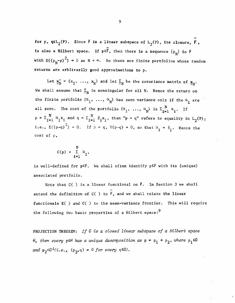
for p, qEL2(P). Since F is a linear subspace of L2(P), its closure, F,
is also a Hubert space. If pCF, then there is a sequence in F
with E((pNp)2) -- 0 as N - . So there are finite portfolios whose random
returns are arbitrarily good approximations to p.
Let x = (x1, ..., x) and let N be the covariance matrix ofxN.
We shall assume that EN is nonsingular for all N. Hence the return on
the finite portfolio ..., has zero variance only if the . are
all zero. The cost of the portfolio (G, ..., ct) Is C. If
= N a0x. and q = E.N1 x., then "p = q" refers to equality in L2(P);
i.e., E((p—q)2) = 0. If p = q, V(p-q) = 0, so that . = .. Hence the
cost of p,
NC(p) =
1=1 1
is well—defined for pEF, We shall often identify pCF with its (unique)
associated portfolio.
ir- -hi1- C( 4c 1ii,r fil rirni1 rn F In Spt-t-icrn h11I —- - —-—
extend the definition of C( ) to F, and we shall relate the linear
functionals E( ) and C( ) to the mean—variance frontier. This will require
the following two basic properties of a Hubert space:9
PROJECTION ThEOR: If C is a closed linecw subspace of a Hubert space
H, then every pEH has a unique decomposition as p = p1 + p2, where p1O
and p2EG(i.e., (p2,q) = 0 for every qCG).

10
RIESZ REPRESENTATION THEOREM: If L is a continuou8 linear functional on
a Hubert apace H, then there i8 a unique qCH auch that L(p) = (q,p) for
every pCI1.
The projection theorem is often used together with the fact that every
finite dimensional subspace is closed. We shall also use the following
two elementary properties of linear functionals:
If G is a linear subspace of a Hilbert space 1-1, then
a linear functional L is continuous on G if and only
if L(pN) - 0 for every sequence in G that converges
to zero;
if G is a linear subspace of a Hubert space 1-1 and if
the linear functiowzl L is continuous on G, then there
is a unique continuous linear functional on the closure
of G that coincides with L on G.
3. ARBITRAGE OPPORTUNITIES AND MEAN-VARIANCE EFFICIENCY
3. 1 Lack of Arbitrage Opportunities
We now consider what it means for there to be no arbitrage opportun-
ities on the asset market. By defining x1 as the return available for
one dollar, we have assumed prices are determined. These prices can be
equilibrium prices if no trader would want to make an infinitely large
trade. We define the absence of arbitrage opportunities in terms of
conditions which, if they failed, would make some risk—averse traders
want to take infinitely large positions.
Let be a sequence of finite portfolios (pCF). Then we shall
say that the market permits no arbitrage opportunities if the following
11
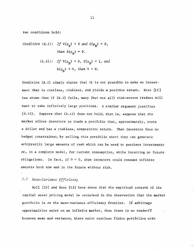
two conditions hold:
Condition (A.i): If V(pN) + 0 and C(pN) - 0,
then E(pN) - 0.
(A.ii): If V(pN) + 0, C(p) 1, and
E(PN)- a, then a > 0.
Condition (A.i) simply states that it is not possible to make an invest-
ment that is costless, riskiess, and yields a positive return. Ross [12]
has shown that if (A.i) fails, many (but not all) risk—averse traders will
ant to take infinitely large positions. A similar argument justifies
(A.ii). Suppose that (A.ii) does not hold; that is, suppose that the
market allows investors to trade aportfolio that, approximately, costs
a dollar and has a riskiess, nonpositive return. Then investors face no
budget constraints; by selling this portfolio short they can generate
arbitrarily large amounts of cash which can be used to purchase investments
or, in a complete model, for current consumption, while incurring no future
obligations. In fact, if a < 0, then investors could consume infinite
amounts both now and in the future without risk.
2 Mean- Variance Efficiency
Roll [10) and Ross [13] have shown that the empirical content of the
capital asset pricing model is contained in the observation that the market
portfolio is on the mean—variance efficiency frontier. If arbitrage
opportunities exist on an infinite market, then there is no tradeoff
between mean and variance; there exist costless finite portfolios with
12
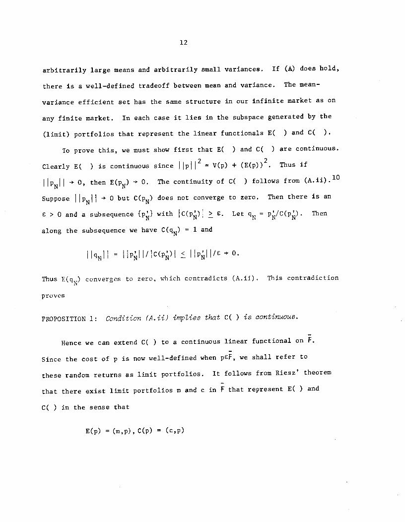
arbitrarily large means and arbitrarily small variances. If (A) does hold,
there is a well—defined tradeoff between mean and variance. The mean—
variance efficient set has the same structure in our infinite market as on
any finite market. In each case it lies in the subspace generated by the
(limit) portfolios that represent the linear functionals E( ) and C( ).
To prove this, we must show first that E( ) and C( ) are continuous.
2 2Clearly E( ) is continuous since J p I
= V(p) + (E(p)) . Thus if
IIPNII - 0, then E(PN) + 0. The continuity of C( ) follows from (A.ii).1°
Suppose INI - 0 but C(pN) does not converge to zero. Then there is an
C > 0 and a subsequence {p} with IC(p)I > C. Let = p/C(p). Then
along the subsequence we have C() 1 and
IIH = IpHflC(p)j IIPII/C 0.
Thus E() converges to zero, which contradicts (A.ii). This contradiction
proves
PROPOSITION 1: condition (A.ii) irplies that C( ) is continuous.
Hence we can extend C( ) to a continuous linear functional on F.
Since the cost of p is now well—defined when pCF, we shall refer to
these random returns as limit portfolios. It follows from Riesz' theorem
that there exist limit portfolios m and c in F that represent E( ) and
C( ) in the sense that
E(p) = (m,p), C(p) = (c,p)
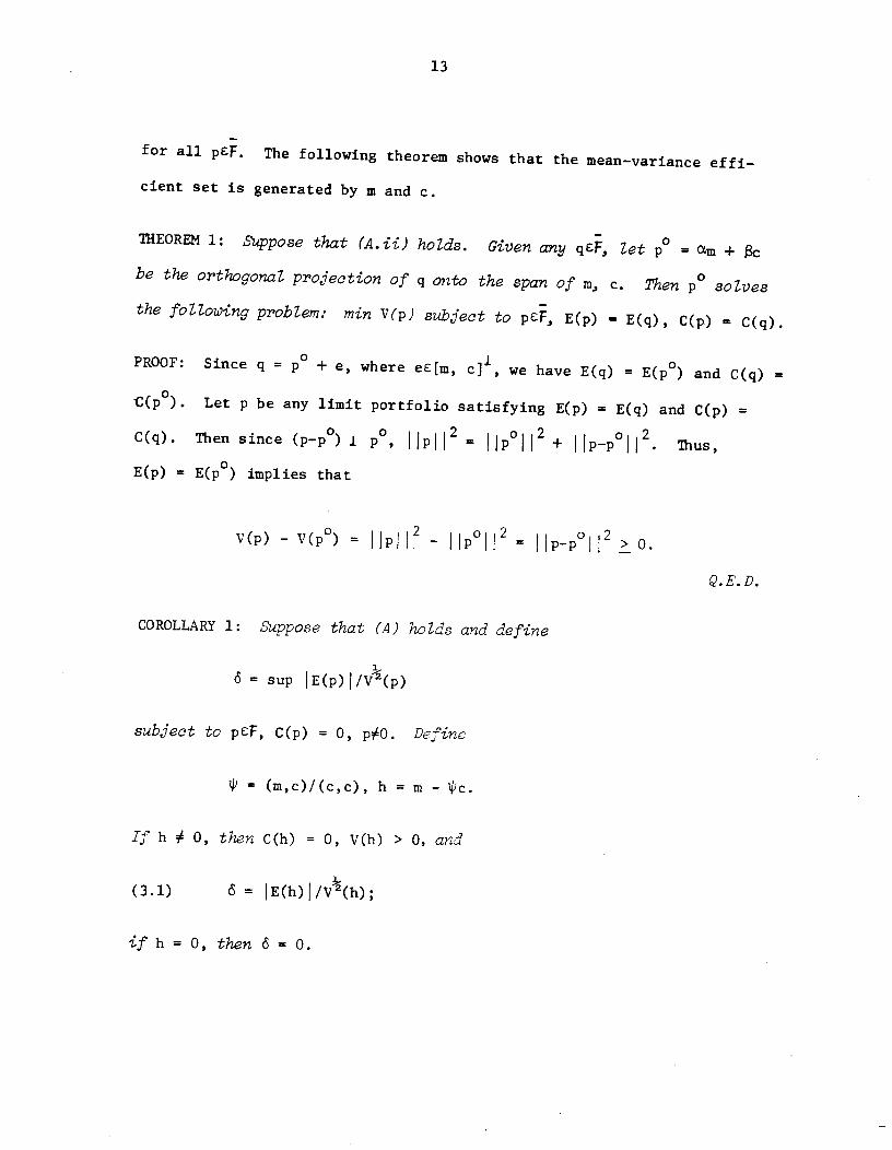
13
for all pCF. The following theorem shows that the mean—variance effi-
cient set is generated by in and c.
THEOREM 1: Suppose that (A.ii) holds. Given any qCF, let p° = am + cbe the orthogonal projection of q onto the span of in, c. Then p° solves
the following problem: mm V(p) subject to pEF, E(p) = E(q), C(p.) = C(q).
PROOF: Since q = p° + e, where eE[m, c]1, we have E(q) = E(p°) and C(q) =
C(p°). Let p be any limit portfolio satisfying E(p) = E(q) and C(p) =
C(q). Then since (p-p°) j p°, Jp 12 = Iip°i 12 +I Jp—p°I 12 Thus,
E(p) = E(p°) implies that
V(p) - V(p°)2 -
I p°J 2 = Ip-p°I 12 >
Q.E.D.
COROLLARY 1: Suppose that (A) holds and define
= sup E(p)J/V(p)
subject to pcF, C(p) = 0, pO. Define
(m,c)/(c,c), h = m — IPc
If h 0, then c(h) = 0, V(h) > 0, and
(3.1) 6 = JE(h)l/V(h);
if h = 0, then 6 = 0.
14
PROOF: If h = 0, then E(p) = 0 whenever C(p) = 0, and so 6 = 0. Suppose
that h # 0. In that case, E(h) # 0, for otherwise (in, h) = 0, (c, h) = 0,
and hC[m, ci imply that h = 0. By (A.i), if E(p) 0 and C(p) = 0, then
V(p) > 0. If C(p) = 0, p # 0, and
IE(p) /v½(p) > E(h) /v(h),
then p = (E(h)/E(p))p has E(p*) = E(h), C(p*) = C(h) = 0, and V(p*) <
V(h). This contradicts Theorem 1 and completes our proof.
Q.E.D.
The parameter 6 gives the slope of the tradeoff between mean and risk
(measured by standard deviation) along the efficient frontier; [hi is the
linear subspace of costless portfolios which are efficient. An investor
can increase risk in an efficient manner by adding a hedge portfolio from
[h] to his holdings. Another way of making this point is to observe that
if p, q[m, c] with C(p) = C(q) = 1, then p — qC[h] and so (3.1) implies
(3.2) E(p) - E(q) = 6V(p-q).
We shall see that 6 plays an important role in our treatment of factor
models.
3.3 Riskiess Asset
In this section we shall examine the implications of the existence of
a riskless limit portfolio.
DEFINITION 1: There is a riskiess limit portfolio if there is a p*CF
with V(p*) = 0 and E(p*) 0.
If (A.ii) holds, then C(p*) is well—defined and C(p*) = 0 violates (A.i).
15
Hence we can set a p*/C(p*). We shall refer to a as a riskiess asset.
If there is an s'CF with C(s') = 1 and V(s') = 0, then C(s-s') = 0,
V(s—s') 0, and (A.i) implies that E(s—s') 0. So $ = a' and the riskiess
asset is unique. Let P = E(s) be the return on the riskless asset; (A.ii)
implies that P > 0.
Note that (sIP, p) = E(p) for all pCF; hence m = s/P. If p[m, c]
and C(p) = 1, then setting q = s in (3.2) gives the following tradeoff
between mean and risk along the efficient frontier:
(3.3) JE(p) — p1 = cSV¾(p).
Thus, if there is a riskiess asset, the frontier of the efficient set (in
(i,o) space) is a straight line rather than a curve as it is usually drawn.
We now develop a necessary and sufficient condition for the existence
of a riskiess asset. We also show that if there is no riskiess limit
portfolio, then the covariance is a natural inner product for the space
F. We use this construction in Section 5. Suppose that there is no
riskiess limit portfolio. Then E(m) 1; for otherwise
E(m) (m, in) = V(m) ÷ (E(m))2
implies that V(m) = 0, a contradiction. If E(m) # 1, then
16
E(p) (m, p) = Cov(m, p) + E(m) E(p)
implies that
E(p) = Cov(m, p)/(l — E(tn)) Cov(m*, p),
where m* = m!(l — E(m)). So we can generate the mean functional from the
covariance with m. If (A) holds, we can also use covariance to generate
the cost functional:
C(p) = (c, p) Cov(c, p) + E(c) E(p)
= Cov(c, p) + E(c)Cov(m*, p) = Cov(c*, p),
where
c' = c + E(c)m*.
Now we have
Hp112 = V(p) + (Cov(m*, p))2 < (1 + V(m*))V(p) (peF),
so that V(p) = 0 implies p = 0. Hence Cov( , ) is an inner product and
) is a norm. Furthermore, if e F and V(pN—pN) ÷ 0 as N, M +
then NN1 4- 0 and, since F is complete under the mean—square norm,
there is a psF with 'N' 4- 0. Hence V(pN-p) ÷ 0 so that F is complete
under the variance norm, and F together with the covariance inner product
forms a Hubert space. Condition (A) is not needed for this result.
17
Note that the span of m*, c is identical to the span of in, c. Let
= Cov(jn*, c*)/V(c*) and h* = — 4*c*. Then h*E4h] since h*C[m, c]
and C(i*) = 0. If h 0 then h* # 0 and
(3.4) = IE(h*)/V(h*) = V½(h*).
We can use the covariance inner product to characterize the existence
of a riskiess asset. If (A) holds and there is no riskless asset, then
we can form the (covariance) orthogonal projection of x. onto c*:
x1 = T c* + w. (i=1,2, ...),
where T = Cov(x., c*)/V(c*) = l/V(c*) and
C(w.) = Cov(c*, w.) = 0. Let be an NX1 vector of ones an( let
=(w1, ..., wN). Then
N £ + v(wN) (N=1,2,
so that has an equicorrelated component. We show now that (3.5) is
also a sufficient condition for there to be no riskless asset.
PROPOSITION 2: Suppose that (A) holds. Then there is no riskiess asset
if and only if there is a > 0 such that
- N N
is positive semi—definite for N=l,2,
18
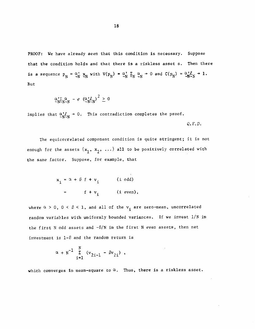
PROOF: We have already seen that this condition is necessary. Suppose
that the condition holds and that there is a riskiess asset s. Then there
is a sequence = x with V(pN) = + 0 and C(PN) = + •But
NNN - (a) >
implies that - 0. This contradiction completes the proof.
Q. E. D.
The equicorrelated component condition is quite stringent; it is not
enough for the assets {x1, x2, .. .} all to be positively correlated with
the same factor. Suppose, for example, that
x. = a + f + v, (1 odd)1 1
f + v. (i even),
where a > 0, 0 < < 1, and all of the v. are zero—mean, uncorrelated
random variables with uniformly bounded variances. If we invest 1/N in
the first N odd assets and —s/N in the first N even assets, then net
investment is l— and the random return is
Na + N1 (v211 — v2.)
1=1
which converges in mean—square to . Thus, there is a riskiess asset.
19
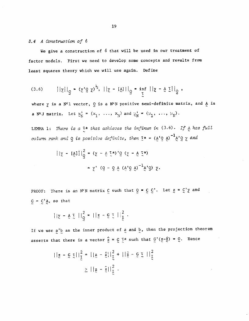
3.4 A Construction of 6
We give a construction of 6 that will be used in our treatment of
factor models. First we need to develop some concepts and results from
least squares theory which we will use again. Define
(3.6) IIHQ (e )½, -[A]IQ
= inf -
where is a <l vector, Q is a NXN positive semi—definite matrix, and A is
a NXJ matrix. Let x (x1, ..., x) and ' 'LEMMA 1: There is a T* that achieves the infinum in (3.6). If A has full
colwnn rank and Q is positive definite, then 1* = (A'Q A)1A'Q y avid
Il — [&II = (y — A I*)'Q (v - A T*)
= y' (Q - Q A (A'Q A)1A'Q) y.
PROOF: There is an N matrix C such that Q = C C'. Let z = C'y and
C = C'A, so that
H- II= il- H.
If we use a'b as the inner product of a and b, then the projection theorem
asserts that there is a vector = C 1* such that G'(z—.) = 0. Hence
— II = — II + — II-
20
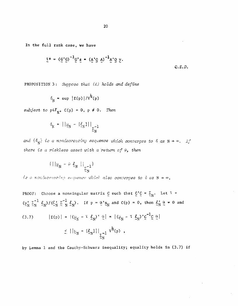
In the full rank case, we have
1* = (G'G)G'z ('Q A)1A'Q y.
Q.E.D.
PROPOSITION 3: Suppose that (A) holds and define
= sup E(p)11V½(p)
subject to PEFN, C(p) = 0, p 0. Then
- N1
and is a nondec eosin sequence which converqe.s to S as N + CO. fthere is a riskiess asset with a ret-urn of p, then
N 1H1}
is cl no2de -ssi s eizc whic7: also conerqes to as N -÷
PROOF: Choose a nonsingular matrix C such that C'C = Let T =
If p = O'XNand C(p) = 0, then 0. = 0 and
(3.7) jE(p) = -' = 1N3-
- 'N —
NE_l V2(p)
by Lemma 1 and the Cauchy—Schwarz inequality; equality holds in (3.7) if
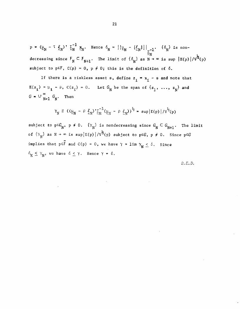
—1= — TN XN. Hence
= N -I
decreasing since C FN+l. The limit of as N -
subject to pCF, C(p) = 0, p 0; this is the definition
If there is a riskiess asset s, define z. = x. — s1 1
E(z.) = p.. — P. C(z.) = 0. Let be the span of {z1,
G=U1GN. Then
21
is non—
is sup E(p)I/V(p)
of ó.
and note that
...,zN} and
-1— — 2 = supjE(p)J1V2(p)
subject to PEGN, o• is nondecreasing since C GN+l. The limit
of as N -* is supE(p)/V½(p) subject to peG, p 0. Since pCG
implies that pF and C(p) = 0, we have y = urn < . SinceN' we have < y. Hence y =
.2.E.D.
22
4. FACTOR STRUCTURE AND ROSS' THEOREM
4.1 Strict Factor Structure
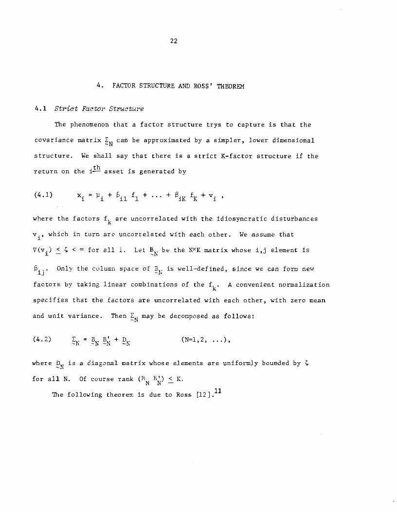
The phenomenon that a factor structure trys to capture is that the
covariance matrix EN can be approximated by a simpler, lower dimensional
structure. We shall say that there is a strict K—factor structure if the
return on the asset is generated by
(4.1) x. = p. + f1 + + iK K +
where the factors are uncorrelated with the idiosyncratic disturbances
v., which in turn are uncorrelated with each other. We assume that1
V(v.) < for all i. Let be the NXK matrix whose i,j element is
Onl' the column space of B is well—defined, since we can form new1j
factors by taking linear combinations of the k A convenient normalization
specifies that the factors are uncorrelated with each other, with zero mean
and unit variance. Then E. may be decomposed as follows:
(4.2) N N N + N (N=l,2, ...),
where is a diagonal matrix whose elements are uniformly bounded by
for all N. Of course rank (RN B') < K.
11The following theorem is due to Ross [12].
23
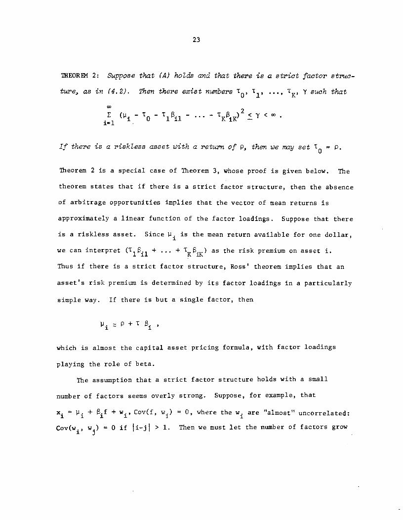
THEOREM 2: Suppose that (A) holds and that there is a strict factor struc-
ture as in (4.2). Then there exist numbers t0T1, ..., Y such that
'o - - ... - tKK)<Y <
If there is a riskiess asset with a return of p, then we may set 10 =
Theorem 2 is a special case of Theorem 3, whose proof is given below. The
theorem states that if there is a strict factor structure, then the absence
of arbitrage opportunities implies that the vector of mean returns is
approximately a linear function of the factor loadings. Suppose that there
is a riskiess asset. Since 1.11 is the mean return available for one dollar,
we can interpret (ti.i + ... + as the risk premium on asset i.
Thus if there is a strict factor structure, Ross' theorem implies that an
asset's risk premium is determined by its factor loadings in a particularly
simple way. If there is but a single factor, then
P + I
which is almost the capital asset pricing formula, with factor loadings
playing the role of beta.
The assumption that a strict factor structure holds with a small
number of factors seems overly strong. Suppose, for example, that
x. = + .f + w, Cov(f, w.) 0, where the w. are "almost" uncorrelated:
Cov(w1, w.) = 0 if i—jl > 1. Then we must let the number of factors grow
24
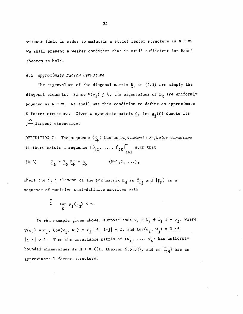
without limit in order to maintain a strict factor structure as N -.We shall present a weaker condition that is still sufficient for Ross'
theorem to hold.
4. 2 Approximate Factor Structure
The eigenvalues of the diagonal matrix in (4.2) are simply the
diagonal elements. Since V(v1) < , the eigenvalues of DN are uniformly
bounded as N - . We shall use this condition to define an approximate
K—factor structure. Given a symmetric matrix C, let g(C) denote its
.thj— largest eigenvalue.
DEFINITION 2: The sequence has an approximate K-factor structure
if there exists a sequence such thati=l
(4.3) N = N B + (N=l,2, ...),
where the 1, j element of the N<Kmatrix BN is .. and {R,) is a
sequence of positive semi—definite matrices with
2. Sup g1(R) < .N
In the example given above, suppose that x = P. + f + w1, where
V(w.) = , Cov(w1, w) = 2 if i—j = 1, and Cov(w, w.) = 0 if
li-il > 1. Then the covariance matrix of (w1, ..., wN) has uniformly
bounded eigenvalues as N -- ([1, theorem 6.5.3]), and so has an
approximate 1—factor structure.
25
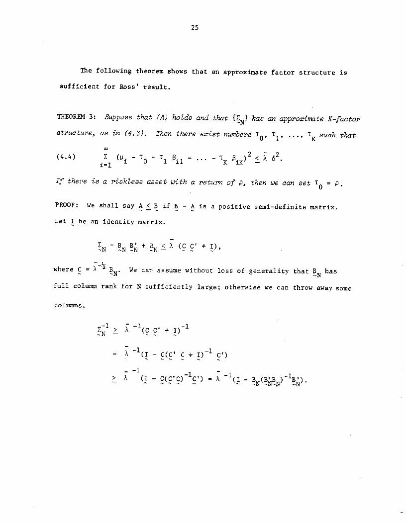
The following theorem shows that an approximate factor structure is
sufficient for Ross' result.
ThEOREM 3: Suppose that (A) holds and that has an approximate K-factor
structure, as in (4.3). Then there exist numbers T, T, such that
(4.4)1=1
- 'o i n - - TK )2 <
If there is a riskiess asset with a return of p, then we can set =
PROOF: We shall say A < B if B — A is a positive semi—definite matrix.
Let I be an identity matrix.
= N N + A (cc' + I),
where C = B. We can assume without loss of generality that RN has
full column rank for N sufficiently large; otherwise we can throw away some
columns.
_1( c' +
= A '( -' +lA (I - C(C'1C') A -
26
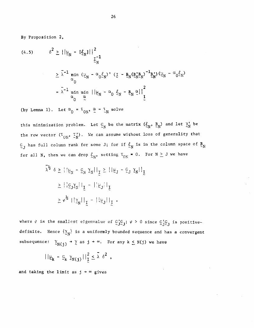
By Proposition 2,
(4.5) ''EN —[N1H2_1
> A1 mm -aON)
- -B (B'B—a0
__l I
2a £ -B a= A mm mm 'N - 0 N Na a I
0 -
ta i a—i solve(by Lemma 1). Le =ON' -.
this minimization problem. Let be the matrix N' and let be
the row vector (TON, T). We can assume without loss of generality that
has full column rank for some J; for N is in the column space of BN
for all N, then we can drop N' setting TON = 0. For N > J we have
1—G H >AII'N
JN' - HJH1
> I iv ii I—' '-NI — 'ZJI
where is the smallest elgenvalue of > 0 since GGJ is positive—
definite. Hence is a uniformly bounded sequence and has a convergent
subsequence: 1N(•) - I as j -3- °. For any k < N(j) we have
kkN(j)'1I a2
and taking the limit as j - gives

27
k
Since this holds for all k, (4.4) follows with to t') =
If there is a riskiess asset, then we can use Proposition 2 to replace
(4.5) by
2 2
N -I_i
then essentially the same argument gives (4.4) with T0 =
Q.E.D.
5. A CHARACTERIZATION OF APPROXIMATE
FACTOR STRUCTURES
We would like to have a simple condition on the {EN} sequence that
implies an approximate K—factor structure, and we would like to know how
to construct the factor loadings (risk premia) from If an approximate
factor structure does exist, we would like to know whether the decomposition
of into {BNB} and {RN} is unique. We shall show that the relevant
condition is that only K of the eigenvalues of are unbounded as N - .Furthermore, there is a unique sequence {BNB} that gives the approximate
factor structure, and it can be obtained from the eigenvectors of {EN}
corresponding to the K largest eigenvalues.
We show first that if there is an approximate K—factor structure, then
only K of the eigenvalues can be unbounded.
28
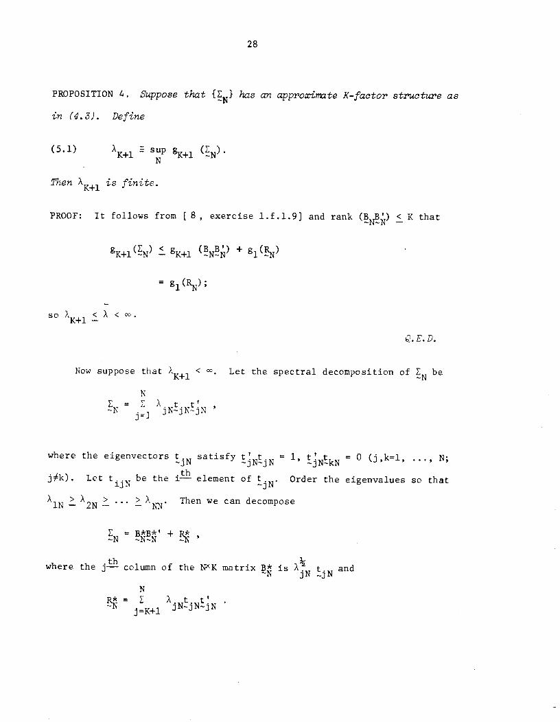
PROPOSITION 4. Suppose that has an approx-inrzte K-factor structure as
in (4.3). Define
(5.1) K+1 K+1
Then is finite.
PROOF: It follows from [ 8, exercise l.f.l.9] and rank (BNB) < K that
- ¼+i +
=gl(RN);
so AK+l X < .
.E.D.
Now suppose that AK÷l < . Let the spectral decomposition of N be
.
where the eigenvectors t.N satisfy =jNLkN
= 0 (j,k=1, ..., N;
thjk). Let tjjN be the i— element of Order the eigenvalues so that
A2N > ... > A. Then we can decompose
= NN +
where the column of the N><K matrix B* is X t. andjN -.jN
=
j=K+1 jNjNjN
29
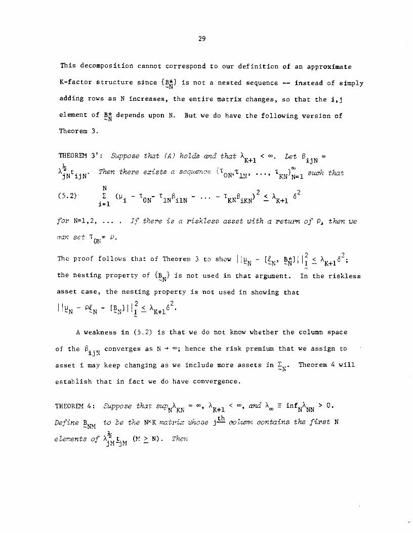
This decomposition cannot correspond to our definition of an approximate
K—factor structure since {B) is not a nested sequence —— instead of simply
adding rows as N increases, the entire matrix changes, so that the i,j
element of B depends upon N. But we do have the following version of
Theorem 3.
ThEOREM 3': Suppose that (A) holds and that ° Let ijN =
AiNtiiN. Then there exists a sequence uI0N,lN, * s7: that
N2 2(5.2) E —
'ON 'lN1 — — 'KNiKN 61=1
for N=l,2 If there is a riskiess asset with a return of P, then we
can . T0= p
The proof follows that of Theorem 3 to show N — N'the nesting property of {BN} is not used in that argument. In the riskless
asset case, the nesting property is not used in showing that
- [N1iIK+l2A weakness in (5.2) is that we do not know whether the column space
of the .. converges as N -* hence the risk premium that we assign toijN
asset i may keep changing as we include more assets in N Theorem 4 will
establish that in fact we do have convergence.
ThEOREM 4: Suppose that 8UPNA= ' < W2 E
1nfNXNN> 0.
Define B to e the NXK matrix whose coiwnn contains the first N
elements of t. (N > N). ThenjMM —

30
has an approximate K-factor structure; i.e., there exists
a sequence i' such that
(N=1,2, ...),
where the i, j element of the NXK matrix is .. and {R} is a sequence
of positive semi-definite matrices whose eigenvalues are uniformly bounded
by AK+l for all N.
(ii) For any N,
NM1N=
(iii) The approximate K-factor structure is unique; i.e., suppose that
there is a seence {y.1, ..., •K1 such that
= NN + (N=1,2, ...),
where the i, j element of the N<K matrixCN
is Y, and is a sequence
of positive semi-definite matrices whose eigenvalues are uniformly bounded
for all N; then
NNNN' NNCOROLLARY 2: Suppose that (A) holds together with the assunrptions of Theorem
4. Then there exist numbers T0 T] ..., such that
i1 '• - — Tlil — — iK - AK+1•
If there is a riskiess asset with a return of P, then we can set =
31
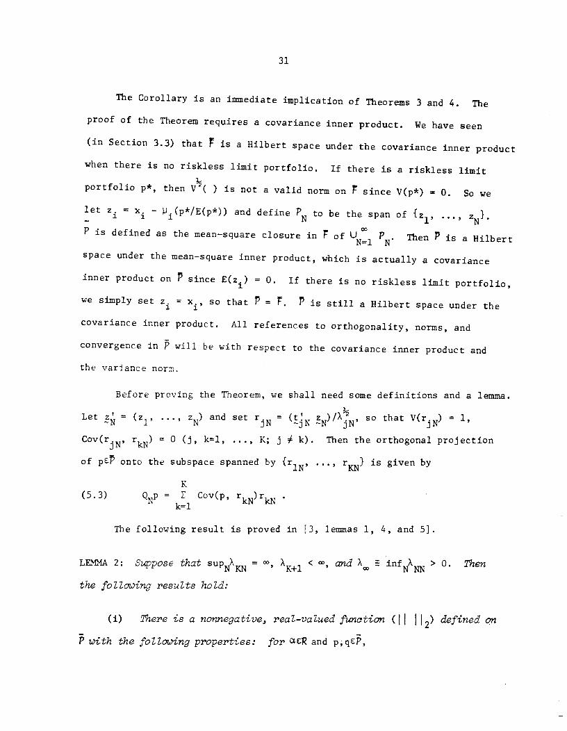
The Corollary is an immediate implication of Theorems 3 and 4. The
proof of the Theorem requires a covariance inner product. We have seen
(in Section 3.3) that is a Hubert space under the covariance inner product
when there is no riskless limit portfolio. If there is a riskless limit
portfolio p*, then V½( ) is not a valid norm on F since V(p*) 0. So we
let z. x. — .(p*/E(p*)) and define to be the span of {1, ..., Z}.1 1 1
00P is defined as the mean—square closure in F of UN1 N Then P is a Hubert
space under the mean—square inner product, which is actually a covariance
inner product on P since E(z.) = 0. If there is no riskless limit portfolio,
we simply set z. x., so that P = F. P is still a Hubert space under the1 1
covariance inner product. All references to orthogonality, norms, and
convergence in P will be with respect to the covariance inner product and
the variance norm.
Before proving the Theorem, we shall need some definitions and a lemma.
Let =(z1, ..., z ) and set r.N = jN N)/XjN so that V(rN) =
N j
Cov(r.N, rkN) = 0 (j, k=l, ..., K; j k). Then the orthogonal projection
of pP onto the subspace spanned by IrlN, ..., r} is given by
K
(5.3) =Cov(p, rkN)r
k= 1
The following result is proved in [3, leimnas 1, 4, and 51.
A <00 andA EinfLEMMA 2: Suppose thatsuPNA}(
=K+l 00 NA
> 0. ThenNN
the following results hold:
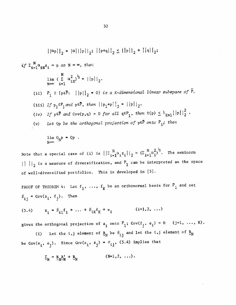
(1) There is a nonnegative, real-valued function (H 112) defined on
P with the following properties: for cXCR and p,qP,
32
llPII2 = IHIPI!2; IIP+Il lPIl2 HqH;
Nf E1=1 + p as N + , thenN
urn ( E iN 2 = Ipi 12N°' 1=1
(ii) P1 {pC: I p 12 = O} is a K—dimensional linear subspace of P.
(iii) If p1P1w2d pEP, then I IP3PI 2= 1' 12
(iv) If pcPd Cov(p,q) = 0 for all q6P1, then V(p) < XK+lI I! I
(v) Let Qp be the orthogonal projection of pEP onto then
urn =
N N 2½Note that a special case of (i) is . c.z.II = (E. ci.) . The setninorm
i=lii 2 i=li
I 2is a measure of diversification, and P1 can be interpreted as the space
of well—diversified portfolios. This is developed in [31.
PROOF OF ThEOR4 4: Let f1, ..., be an orthonormal basis for P1 and set
= Cov(z., f.). Then1J 1- J
(5.4) z. = + + KK + e. (i1,2, ...)
gives the orthogonal projection of z. onto P1; Cov(f., e1)= 0 (j1, ..., K).
(i) Let the i,j element of be .. and let thei,j element of RN
be Cov(e.., e.). Since Cov(z1, z.) = 0.., (5.4) implies that
= NN + R.N (N=l, 2, ...).
33
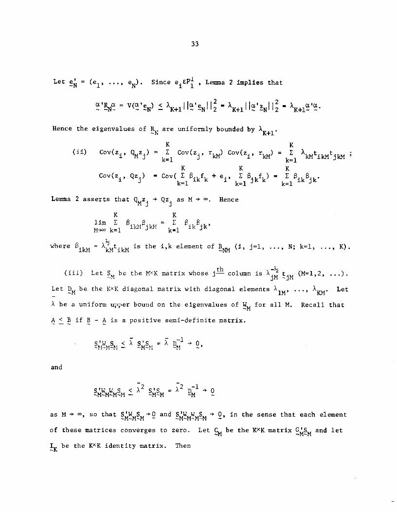
Let =(e1, ..., es). Since e1CP , Lemma 2 Implies that
cRNc = +1! I'I I = AK+lI 1N' 2
Hence the eigenvalues of are uniformly bounded by AK+l.
(ii) Cov(z, QMZJ) = k=1C:v(z, r) Cov(z., r) =
k=1 AtMtjCov(z., Qz.) = Cov( E + e., E kk =1 k=l 1 1 k=l k=1
1 3
Lemma 2 asserts that QMz. + Qz. as M -3- . Hence
k=li1ijI =
k=l ikjk'
where = ANt is the i,k element of B (1, j=l, ..., N; k1, ..., K).
(iii) Let SM be the MXK matrix whose column is (M1,2, ...).
Let be the KXK diagonal matrix with diagonal elements AiM, ..' A. Let
A be a uniform upper bound on the eigenvalues of for all M. Recall that
A < B if B — A is a positive semi—definite matrix.
1MM — A
and
MMMM < = 2 D' 9
as N -s- , so that SWMSM+O and SWMWMSM -3- 0, in the sense that each element
of these matrices converges to zero. Let be the KXK matrix GSM and let
be the KXK identity matrix. Then

34
= MMM =MMM + MMM
implies that CCM ÷ 'K as N -* . Hence the elements of CM are uniformly
bounded for all M, and {CM} has a convergent subsequence: M(j) - as
K implies that C' C1 and so =
Recall that is the NXK matrix whose column contains the first
N elements of ) t. (M > N). ThenjMjM —
MM= MN +
= MN +
implies that
NN NN +
where H is the NXK matrix that contains the first N rows of WNSM.
ThfNN — M1MM
implies that 0 as N c and so HH 0. Since {CM} is uniformly
bounded, GNCMH - 0 as M - . Hence part (ii) of the Theorem gives
NNNN
= =
It follows that
Q.E.L.
35
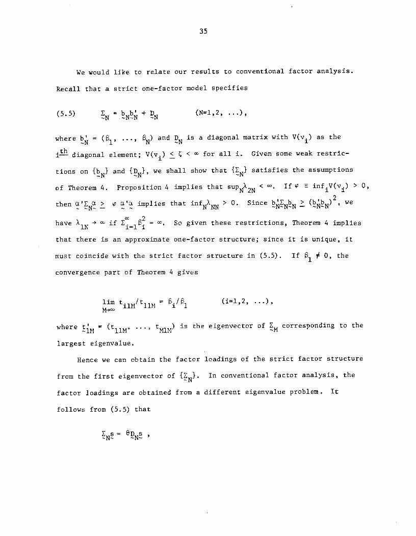
We would Like to relate our results to conventional factor analysis.
Recall that a strict one—factor model specifies
(55) =bNb + (N=l,2, ...),
where b (, ••• ) and is a diagonal matrix with V(v) as the
•thi— diagonal element; V(v) < < for all i. Given some weak restric-
tions on {bN} and {DN}, we shall show that {EN} satisfies the assumptions
of Theorem 4. Proposition 4 implies that supNX2N < co• If P inf1V(v1) > 0,
then > p cX'3 implies that infNA > 0. Since bENbN we
Co 2have Co f = °. So given these restrictions, Theorem 4 implies
that there is an approximate one—factor structure; since it is unique, it
must coincide with the strict factor structure in (5.5). If 0, the
convergence part of Theorem 4 gives
urn tilM/tllN = iIl (11,2, ...),
wheretiM
= (tl1M ..., tflJ4) is the elgenvector of EM corresponding to the
largest elgenvalue.
Hence we can obtain the factor loadings of the strict factor structure
from the first eigenvector of In conventional factor analysis, the
factor loadings are obtained from a different eigenvalue problem. It
follows from (5.5) that
=
36
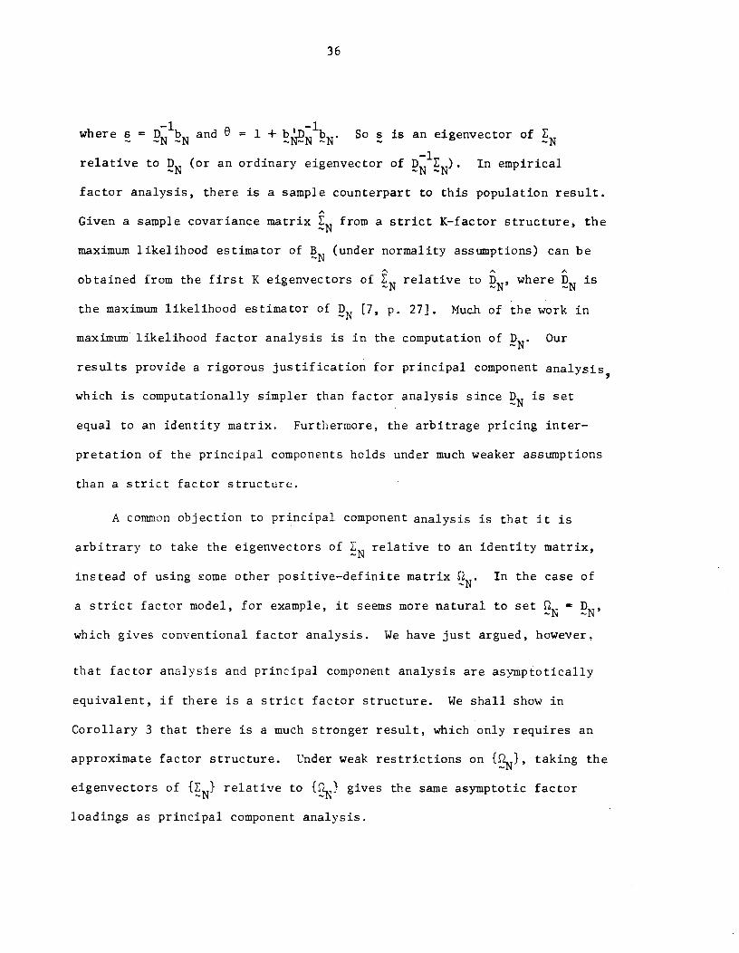
where s =DN1bN
and = 1 + So s is an eigenvector of EN
relative to (or an ordinary elgenvector of DN'EN). In empirical
factor analysis, there is a sample counterpart to this population result.
Given a sample covariance matrix N from a strict K—factor structure, the
maximum likelihood estimator of (under normality assumptions) can be
obtained from the first K eigenvectors of EN relative to where is
the maximum likelihood estimator of DN [7, p. 27]. Much of the work in
maximum likelihood factor analysis is in the computation of DN. Our
results provide a rigorous justification for principal component analysis
which is computationally simpler than factor analysis since is set
equal to an identity matrix. Furthermore, the arbitrage pricing inter-
pretation of the principal components holds under much weaker assumptions
than a strict factor structure.
A common objection to principal component analysis is that it is
arbitrary to take the eigenvectors of relative to an identity matrix,
instead of using some other positive—definite matrix N• In the case of
a strict factor model, for example, it seems more natural to set N =
which gives conventional factor analysis. We have just argued, however,
that factor analysis and principal component analysis are asymptotically
equivalent, if there is a strict factor structure. We shall show in
Corollary 3 that there is a much stronger result, which only requires an
approximate factor structure. Under weak restrictions on {}, taking the
eigenvectors of relative to 2N} gives the same asymptotic factor
loadings as principal component analysis.
37
Let be a nested sequence of positive—definite matrices, with
eigenvalues uniformly bounded away from 0 and : infg() > 0,
pl suP1(c) < the i, j element of ft is L) There exists aij•
nonsingular matrix such that
NNN =9N' NNN
1 elements U > > S . Letwhere 0N is a diagonal matrix with diagona iN — —
ths be the j— column of Then-jN
NS = = s-N N -N N-NN
so that is an eigenvector of relative to
We can use these eigenvectors to obtain an alternative arbitrage
pricing formula. Since
=-'N NNNIN
we have
Nth
where is the NXK matrix whose j— column is t = ONSiN and-j N
N
j=K+l0jNNjNjNN
toAssume that AK+l < we shall see below thaK+l,N _? XK+l• Hence
38
X1E jNjNN
—1 —l= A1c2 AK+lPl
Then, just as with Theorem 3', we can follow the proof of Theorem 3 to
obtain
(5.6) (Pi_TON_TlNlN— }AKN AK+ll
for N=l,2, .... where jN is the i,j element of B.
The objection that principal component analysis is arbitrary is
relevant in our context only if the column space of still depends
upon {2N) in the limit as N - The following result shows that it
does not.
COROLLARY 3: Suppose that satisfies the assumptions of Theorem 4 and
that E suPg1(Q) < , infg() > 0. Let {BNBI} be defined as
in Theorem 4 and define B to be the NXK matrix whose j--- column contains
the first N elements of (N > N). Then
urn BB = BNB (N1,2, ...),
which does not depend upon
PROOF. Recall that a sequence of matrices {A} is nested if the i,j element
of AN does not depend upon N. We can recursively form a nested sequence
39
of upper—triangular, nonsingular matrices such that Cf2NCN N for all
N; the i,j element of is with = 0 for I > i. Let N = NNNand = NN Then = N!N' so that is an eigenvalue of ZN, with
= NjN as the corresponding eigenvector. Note that NjN =
jNkN= 0 (j,k = 1, ..., N; jk). We need to show that {EN} satisfies the
assumptions of Theorem 4. is a sequence of positive—definite, nested
matrices since the CN are nonsingular, upper—triangular, and form a nested
sequence. Let C be a NX(k—l) matrix and let be a NX1 vector; it follows
from [8 , lf.2.iii] that
a' a
kN = inf supG G'CO
The substitution H = C1G,= C gives
___OkN
=
I(\
Since
inf supH H'=O
and < < we have
l'kN 0kN cxkN (k=l, ..., N).
Hence supNO} = SUPNOK+1N< and infNO >
So we can apply Theorem 4 to conclude that {EN} has an approximate
K—factor structure:
40
NN + (N=l, 2, ...),
and
where B is the NXK matrix whose j-- column contains the first N elements
of°MEjM
(N N). Hence
(5.7) = +
Note that {Cl1BN is a sequence of nested matrices, since is nested
and {c1} is nested and lower—triangular.
Since
the uniform upper bound on g1() implies that the eigenvalues of C'RNC
are uniformly bounded for all N, which implies that (5.7) gives an approximate
K—factor structure for Then the uniqueness result in Theorem 4 shows
that
= NN
Since is lower—triangular and C11B = , we have = C1BW.
Hence
= i1(j )C =Q. E. D.
41
FOOTNOTES
'We are indebted to Bob Anderson, Steve Ross, Jose Scheinkman, and
particularly to Jim Mirrlees for helpful suggestions, and to the National
Science Foundation and the University of Wisconsin Graduate School for
research support. Chamberlain held an Alfred P. Sloan Research Fellowship
and Rothschild held the Oskar Morgenstern Distinguished Fellowship at
Mathematica while some of the work on this paper was done. The research
reported here is part of the NBER's program in Financial Markets and
Monetary Economics. Any opinions expressed are those of the authors and
not those of the National Bureau of Economic Research.
2That is, the covariance matrix of asset returns may be written as the
sum of a diagonal matrix and a matrix of short rank as in equation (1.2)
below.
3Chamberlain requires that there be a mean—variance efficient portfolio
which is so well—diversified that it contains only factor variance and no
idiosyncratic variance. Connor requires that the supply of the assets be
well—diversified.
4See [2] and [10] for the case with a finite number of assets.
5Since all assets cost a dollar, a formula which explains the mean
return of the i' asset is an asset pricing formula; it determines the
mean return per dollar spent on asset 1. If there is a riskiess asset with
rate of return P, then 1J — P is the risk premium which investors get if
they buy asset i.
42
6We assume also that the smallest eigenvalue of ZN is uniformly
bounded away from zero for all N.
7Let {GN} be a sequence of matrices where has rN rows and
columns. Then {GN} is a nested sequence if the rN by CN upper left—hand
submatrix of N+l is G. Clearly {BN} and {EN} (of both (1.2) and (1.3))
are nested.
and Ross [11] have used factor analysis in their empirical work
on arbitrage pricing.
9See, for example, [9, Chapters I and II].
10The relationship between arbitrage and the continuity of price
functionals is examined in a more general setting by Kreps [6].
See Huberman 15] for an alternative proof.
43
REFERENCES
[1] Anderson, T. W.: The Statistical Analysis of Time Series. New York:
Wiley, 1971.
[2] Chamberlain, C.: "A Characterization of the Distributions that Imply
Mean—Variance Utility Functions," University of Wisconsin—Madison,
Social Systems Research Institute Workshop Series No. 8027,
1980; Journal of Economic Theory, forthcoming.
[3] __________: "Funds, Factors, and Diversification in Arbitrage Pricing
Models," University of Wisconsin—Madison, Social Systems Research
Institute Workshop Series 8222, 1982.
[4] Connor, G.: "Asset Prices in a Well—Diversified Economy," Yale
University Technical Paper No. 47, 1980.
[5] Huberman, G.: "A Simple Approach to Arbitrage Pricing Theory,"
Journal of Economic Theory, forthcoming.
[6] Kreps, D. N.: "Abritrage and Equilibrium in Economies with Infinitely
Many Coodities," Journal of Mathematical Economics, 8 (1981),
15—35.
[7] Lawley, D. N. and A. E. Maxwell: Factor Analysis as a Statistical
Method. New York: Elsevier, 1971.
[8] Rao, C. R.: Linear Statistical Inference and Its Applications, 2nd
edition. New York: Wiley, 1973.
[9] Reed, M. and B. Simon: Methods of Modern Mathematical Physics.
I: Functional Analysis. New York: Academic Press, 1972.
44
[10) Roll, R.: "A Critique of the Asset Pricing Theory's Tests. Part I:
On Past and Potential Testability of the Theory," Journal of
Financial Economics, 4 (1977), 129—176.
[11) Roll, R. and S. A. Ross: "An Empirical Investigation of the Arbitrage
Pricing Theory," Journal of Finance, 5 (1980), 1073—1103.
[12] Ross, S. A.,, "The Arbitrage Theory of Capital Asset Pricing," Journal
of Economic Theory, 13 (1976), 341—360.
[13] _________: "The Capital Asset Pricing Model (CAPM), Short—Sale
Restrictions, and Related Issues," Journal of Finance, 32 (1977),
177—183.
[14] __________: "Return, Risk, and Arbitrage," in Risk and Return in
Finance, I, ed. by I. Friend and J. L. Bicksier., Cambridge,
Mass.: Ballinger, 1977.
Recommended