NBER WORKING PAPER SERIES

SETTING THE X FACTOR INPRICE CAP REGULATION PLANS

Jeffrey I. BernsteinDavid E.M. Sappington

Working Paper 6622http://www.nber.org/papers/w6622

NATIONAL BUREAU OF ECONOMIC RESEARCH1050 Massachusetts Avenue

Cambridge, MA 02138June 1998

We thank Lloyd Benbow, Michael Cavell, Kenneth Gordon, Willie Grieve, Stanford Levin, DonRomaniuk, and Dennis Weisman for helpful discussion and insights. Any opinions expressed arethose of the author and not those of the National Bureau of Economic Research.

© 1998 by Jeffrey I. Bernstein and David E.M. Sappington. All rights reserved. Short sections oftext, not to exceed two paragraphs, may be quoted without explicit permission provided that fullcredit, including © notice, is given to the source.

Setting the X Factor in Price Cap Regulation PlansJeffrey I. Bernstein and David E.M. SappingtonNBER Working Paper No. 6622June 1998JEL No. LSI, D24

ABSTRACT

Despite the popularity of price cap regulation in practice, the economic literature provides

relatively little guidance on how to determine the X factor, which is the rate at which inflation -

adjusted output prices must fall under price cap plans. We review the standard principles that inform

the choice of the X factor, and then consider important extensions. We analyze appropriate

modifications of the X factor: (1) when only a subset of the firm's products are subject to price cap

regulation, and when product-specific costs and productivity cannot be measured; (2) when the

pricing decisions ofthe regulated firm affect the economy-wide inflation rate; and (3) in the presence

of structural changes in the industry, such as a strengthening of competitive forces.

Jeffrey I. BernsteinDepartment of EconomicsCarleton University1125 Colonel By DriveOttawa, Ontario KIS 5B6CanadaandNBERjefebernstein@carleton.ca

David E.M. SappingtonDepartment of EconomicsUniversity of Florida224 Matherly HallGainesville, FL 32611-2017

1. Introduction.

Price cap regulation has become a popular form of regulation in many markets. For instance,

most state governments in the United States employ some form of price cap regulation to govern

the intrastate activities of their telecommunications suppliers (Kirchhoff, 1998a,b). Price cap

regulation typically specifies a rate at which the prices that a regulated firm charges for its services

must decline, on average, after adjusting for inflation. The required rate of price decline is

divorced from the firm's realized production costs and earnings, at least in theory. By severing

the link between authorized prices and realized costs -- a link that is a defining feature of rate-of-

return regulation -- price cap regulation can provide the regulated firm with stronger incentives

to reduce production costs and improve its operating efficiency than does rate-of-return

regulation. 1

The rate at which the firm's inflation-adjusted output prices must decline is commonly referred

to as the Xfactor. Regulators routinely specify a value for the X factor when they implement price

cap regulation, but they are forced to do so with little guidance from the economic literature. The

literature provides useful discussions of the advantages and disadvantages of price cap regulation,

and offers some useful insights regarding the general structuring of price cap plans? However,

the literature provides surprisingly little guidance on how to determine what is arguably the most

critical feature of price cap regulation -- the rate at which inflation-adjusted prices must decline.

The purpose of this paper is to help fill this significant void in the literature.

1. For example, see Armstrong et al. (1994) and Sappington and Weisman (1996), and thereferences cited therein.

2. See, for example, Beesley and Littlechild (1989), Braeutigam and Panzar (1989), Brennan(1989), Cabral and Riordan (1989), Lewis and Sappington (1989), Schmalensee (1989), andPint (1992).

- 2 -

We begin in section 2 by reviewing how to calculate the X factor in a simple benchmark setting

where all of the regulated firm's services are subject to price cap regulation, where the economy-

wide rate of output price inflation is not affected by prices set in the regulated industry, and where

no significant structural change is anticipated in the regulated industry. We show that in this

benchmark setting, the X factor reflects the extent to which: (1) the total factor productivity growth

rate in the regulated industry exceeds the corresponding growth rate in the rest of the economy;

and (2) the prices of inputs employed by firms in the regulated industry are rising less rapidly than

the prices of inputs employed by other firms in the economy. 3

Section 3 begins our analysis of appropriate changes to the X factor in more realistic settings.

We derive the relevant changes when: (1) s'ome, but not all, of the regulated firm's services are

subject to price cap regulation; and (2) the prices set by the regulated firm affect the rate of output

price inflation elsewhere in the economy. In the telecommunications industry, only a subset of the

regulated firm's services are typically subjected to price cap regulation. Furthermore, joint

products and common factors of production preclude the measurement of product-specific

productivity and input price growth rates. Consequently, corrections to the standard X factor to

account for a limited span of regulatory control are both important and subtle. In the electric

power and telecommunications industries, the primary outputs of the regulated firm are often

important inputs for other producers. Since output price inflation in the economy is influenced by

changes in input prices, the regulated firm's pricing decisions will influence the realized economy-

wide inflation rate when the firm's outputs are inputs in other sectors. The standard X factor

3. This conclusion (reported in Kwoka (1990), for example) presumes that extranormal profitis zero both in the regulated industry and elsewhere in the economy. We derive the necessarymodifications to this conclusion when the zero-profit assumption is not imposed.

- 3 -

requires modification in the presence of such influence.

In section 4, we examine the modifications of the X factor that are required to account for

structural shifts in industry conditions due, for example, to changes in regulatory regime or

changes in the strength of competitive forces. Increased competition in the industry and/or the

adoption of incentive regulation can induce an incumbent supplier to operate more efficiently and

thereby increase its total factor productivity growth rate. Consequently, such changes can justify

a higher X factor (i.e., a more rapid decline in inflation-adjusted prices) than historical

performance would suggest. However, the impact of competition on the productivity growth rate

of an incumbent supplier, and thus on the most appropriate X factor, is not unequivocal. We show

that strengthening competitive forces can justify a decrease in the rate at which the prices of

regulated services must decline under price cap regulation (i.e., a reduction in the X factor), at

least in the short run. We provide an explicit characterization of the many diverse ways in which

strengthening competitive forces affect the most appropriate X factor.

The analysis in sections 2 through 4 abstracts from some real-world concerns in order to keep

the analysis tractable. Some of these additional concerns, such as service quality and unanticipated

shocks to the regulated firm's revenues or costs, are discussed briefly in the concluding section,

section 5.

2. The Basic Principles Underlying Price Cap Regulation.

The purpose of price cap regulation, like many forms of regulation, is to replicate the discipline

that market forces would impose on the regulated firm if they were present. Therefore, to

understand the basic design of price cap regulation, it is important to understand the discipline that

market forces impose. A primary effect of market forces is to limit the rate of growth of a firm's

- 4 -

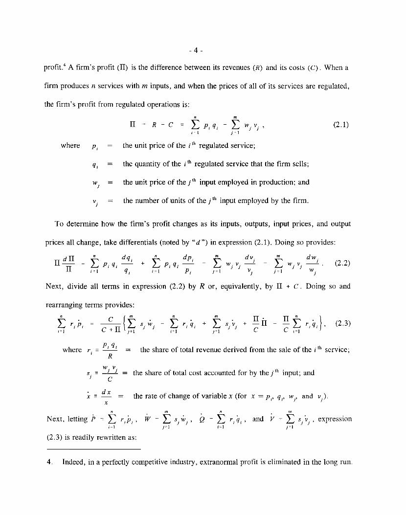
profit. 4 A firm's profit (II) is the difference between its revenues (R) and its costs (C). When a

firm produces n services with m inputs, and when the prices of all of its services are regulated,

the firm's profit from regulated operations is:

n m

II = R - C = L Pi qi - Li = I j = 1

w. v.J J

(2.1)

where Pi

q, =

w. =J

VJ

the unit price of the i th regulated service;

the quantity of the i th regulated service that the firm sells;

the unit price of the j th input employed in production; and

the number of units of the j th input employed by the firm.

To determine how the firm's profit changes as its inputs, outputs, input prices, and output

prices all change, take differentials (noted by "d") in expression (2.1). Doing so provides:

II dii n dqi n dP im dv m dw.

= LPiqi- + LP,qi- - L w.v. _J - L w v.__J (2.2)

II J J J Ji == 1 q, i == I Pi J = I V j = I w.

J J

Next, divide all terms in expression (2.2) by R or, equivalently, by II + C. Doing so and

rearranging terms provides:n

L riP i =;=1

(2.3)

where r,-R

= the share of total revenue derived from the sale of the i th service;

w. v.s. - _J_J =J C

dxx= =

x

the share of total cost accounted for by the j th input; and

the rate of change of variable x (for x = Pi' qi' Wi' and v).

n

Next, letting P = L r,p" Wi=1

(2.3) is readily rewritten as:

m

L sjWJ ' Qr 1

n

L riq" and Vi cc l

m

L Sj vJ

' expressionjel

4. Indeed, in a perfectly competitive industry, extranormal profit is eliminated in the long run.

p

- 5 -

(2.4)

(2.5)

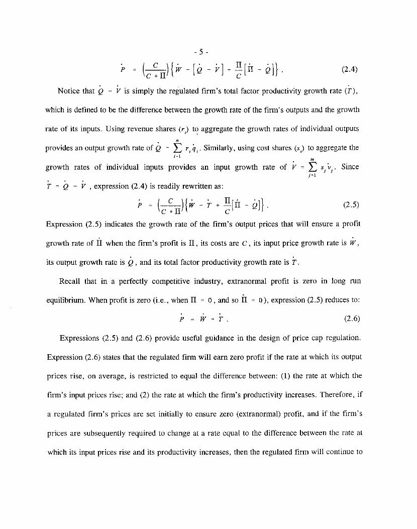
. .Notice that Q - V is simply the regulated firm's total factor productivity growth rate (T),

which is defined to be the difference between the growth rate of the firm's outputs and the growth

rate of its inputs. Using revenue shares (r.) to aggregate the growth rates of individual outputsI •

n

provides an output growth rate of il = L r i qi. Similarly, using cost shares (s) to aggregate the;::01

m

growth rates of individual inputs provides an input growth rate of V = L sJ v). Sincej=1

T = Q - V , expression (2.4) is readily rewritten as:

p = (C~II){W - T + ~[ir - ill}.Expression (2.5) indicates the growth rate of the firm's output prices that will ensure a profit

. .growth rate of II when the firm's profit is II, its costs are C, its input price growth rate is w,

. .its output growth rate is Q, and its total factor productivity growth rate is T.

Recall that in a perfectly competitive industry, extranormal profit is zero in long run

equilibrium. When profit is zero (i.e., when II = 0, and so II 0), expression (2.5) reduces to:

p = W - T . (2.6)

Expressions (2.5) and (2.6) provide useful guidance in the design of price cap regulation.

Expression (2.6) states that the regulated firm will earn zero profit if the rate at which its output

prices rise, on average, is restricted to equal the difference between: (1) the rate at which the

firm's input prices rise; and (2) the rate at which the firm's productivity increases. Therefore, if

a regulated firm's prices are set initially to ensure zero (extranormal) profit, and if the firm's

prices are subsequently required to change at a rate equal to the difference between the rate at

which its input prices rise and its productivity increases, then the regulated firm will continue to

- 6 -

earn zero extranormal profit, just as it would in a competitive market place.s

Of course, if price cap regulation were to proceed first by measuring actual changes in the

regulated firm's input prices and productivity and then by adjusting the firm's output prices

accordingly, price cap regulation would function much like rate-of-return regulation. In particular,

the regulated firm would have limited financial incentive to improve its productivity, since any

realized productivity gains would generate offsetting price reductions. To provide incentives for

productivity gains, price cap regulation should require the regulated firm's prices to vary with

projected, not actual, changes in the firm's productivity and input prices. Under such a policy, the

firm will gain financially if it achieves productivity growth that exceeds expectations and will

suffer financially if its productivity growth falls short of expectations. Consequently, the firm will

face strong incentives to operate diligently and to secure productivity gains.

The longer is the time period over which a firm's authorized prices are divorced from its

realized production costs, the stronger are the firm's incentives to reduce its production costs and

enhance its productivity. However, if authorized prices are linked solely to imperfect projections

of likely productivity gains and input price movements for long periods of time, then actual profit

and performance levels can deviate substantially from predicted levels.6 To limit the extent of such

deviations, it is useful to base ongoing pricing restrictions in price cap regulation plans on

updated, current measures of relevant variables. A particularly important variable that is often

5. Expression (2.5) reveals the r~quisite adjustment in the firm's output price growth rate toensure a profit growth rate of II when the firm's profit is II. Notice, for instance, that whenII > 0, a higp.er output price growth rate is required to sustain a strictly positive profitgrowth rate (II > 0), ceteris paribus.

6. See Schmalensee (1989).

- 7 -

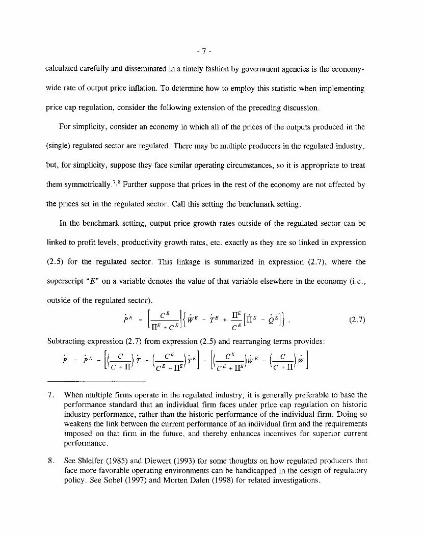
calculated carefully and disseminated in a timely fashion by government agencies is the economy-

wide rate of output price inflation. To determine how to employ this statistic when implementing

price cap regulation, consider the following extension of the preceding discussion.

For simplicity, consider an economy in which all of the prices of the outputs produced in the

(single) regulated sector are regulated. There may be multiple producers in the regulated industry,

but, for simplicity, suppose they face similar operating circumstances, so it is appropriate to treat

them symmetrically.7,s Further suppose that prices in the rest of the economy are not affected by

the prices set in the regulated sector. Call this setting the benchmark setting.

In the benchmark setting, output price growth rates outside of the regulated sector can be

linked to profit levels, productivity growth rates, etc. exactly as they are so linked in expression

(2.5) for the regulated sector. This linkage is summarized in expression (2.7), where the

superscript "E" on a variable denotes the value of that variable elsewhere in the economy (i.e.,

outside of the regulated sector).

pE = [IIEC+Ecel{ WE - TE+ ~: lip _ QE]} .

Subtracting expression (2.7) from expression (2.5) and rearranging terms provides:

p = pE - [(C ~ II) T - (CEc+EIIE)TE] - [(CEC+EIIE)WE - (C ~ II) w]

(2.7)

7. When multiple firms operate in the regulated industry, it is generally preferable to base theperformance standard that an individual firm faces under price cap regulation on historicindustry performance, rather than the historic performance of the individual firm. Doing soweakens the link between the current performance of an individual firm and the requirementsimposed on that firm in the future, and thereby enhances incentives for superior currentperformance.

8. See Shleifer (1985) and Diewert (1993) for some thoughts on how regulated producers thatface more favorable operating environments can be handicapped in the design of regulatorypolicy. See Sobel (1997) and Morten Dalen (1998) for related investigations.

- 8 -

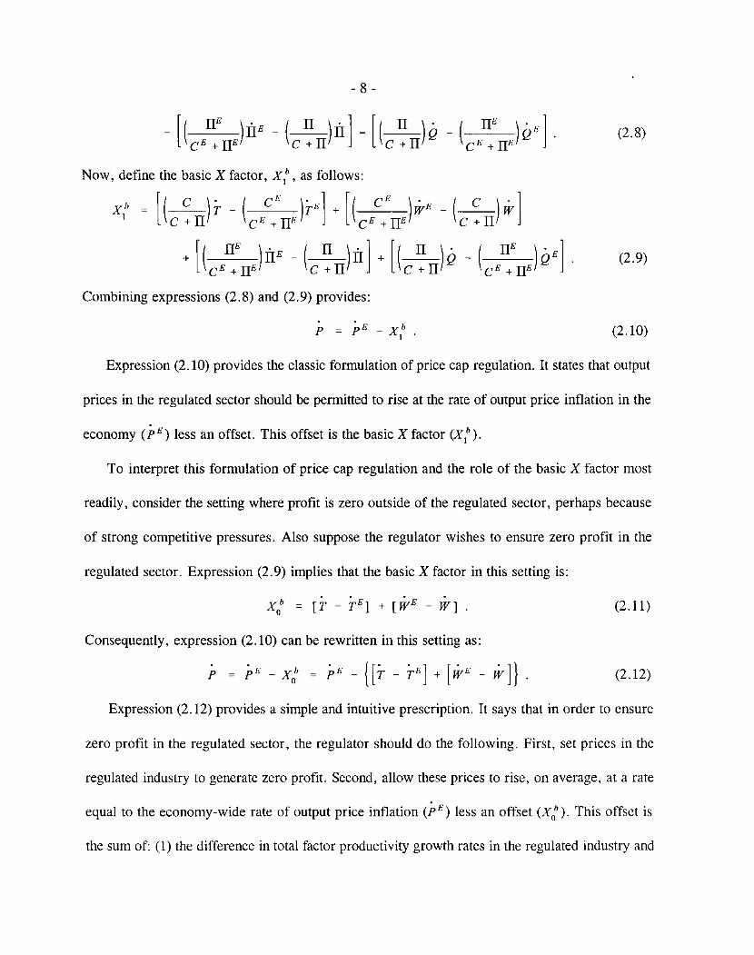
Now, define the basic X factor, X]b, as follows:

xt = [(C ~rr)T - (CEC+ErrJTE] + [(CEC:rrJWE - (C ~rr)W]

+ [(CE~ErrJirE - (C ~rr)ir) + [(C ~rr)Q - (CE~ErrJQE] (2.9)

Combining expressions (2.8) and (2.9) provides:

(2.10)

Expression (2.10) provides the classic formulation of price cap regulation. It states that output

prices in the regulated sector should be permitted to rise at the rate of output price inflation in the

economy (p E) less an offset. This offset is the basic X factor (X]b).

To interpret this formulation of price cap regulation and the role of the basic X factor most

readily, consider the setting where profit is zero outside of the regulated sector, perhaps because

of strong competitive pressures. Also suppose the regulator wishes to ensure zero profit in the

regulated sector. Expression (2.9) implies that the basic X factor in this setting is:

(2.11)

Consequently, expression (2.10) can be rewritten in this setting as:

(2.12)

Expression (2.12) provides a simple and intuitive prescription. It says that in order to ensure

zero profit in the regulated sector, the regulator should do the following. First, set prices in the

regulated industry to generate zero profit. Second, allow these prices to rise, on average, at a rate

equal to the economy-wide rate of output price inflation (pE) less an offset (X;). This offset is

the sum of: (1) the difference in total factor productivity growth rates in the regulated industry and

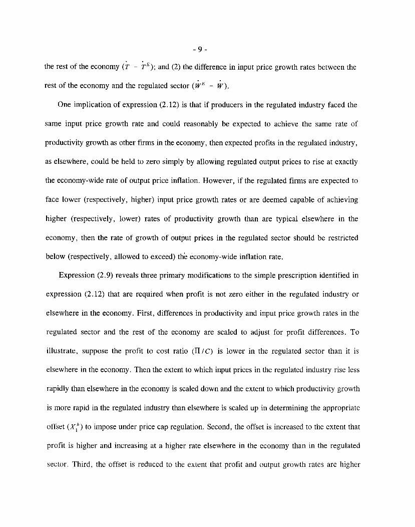
- 9 -

the rest of the economy (T - TE); and (2) the difference in input price growth rates between the

rest of the economy and the regulated sector (fvE- W).

One implication of expression (2.12) is that if producers in the regulated industry faced the

same input price growth rate and could reasonably be expected to achieve the same rate of

productivity growth as other firms in the economy, then expected profits in the regulated industry,

as elsewhere, could be held to zero simply by allowing regulated output prices to rise at exactly

the economy-wide rate of output price inflation. However, if the regulated firms are expected to

face lower (respectively, higher) input price growth rates or are deemed capable of achieving

higher (respectively, lower) rates of productivity growth than are typical elsewhere in the

economy, then the rate of growth of output prices in the regulated sector should be restricted

below (respectively, allowed to exceed) the economy-wide inflation rate.

Expression (2.9) reveals three primary modifications to the simple prescription identified in

expression (2.12) that are required when profit is not zero either in the regulated industry or

elsewhere in the economy. First, differences in productivity and input price growth rates in the

regulated sector and the rest of the economy are scaled to adjust for profit differences. To

illustrate, suppose the profit to cost ratio (II / C) is lower in the regulated sector than it is

elsewhere in the economy. Then the extent to which input prices in the regulated industry rise less

rapidly than elsewhere in the economy is scaled down and the extent to which productivity growth

is more rapid in the regulated industry than elsewhere is scaled up in determining the appropriate

offset (X1h

) to impose under price cap regulation. Second, the offset is increased to the extent that

profit is higher and increasing at a higher rate elsewhere in the economy than in the regulated

sector. Third, the offset is reduced to the extent that profit and output growth rates are higher

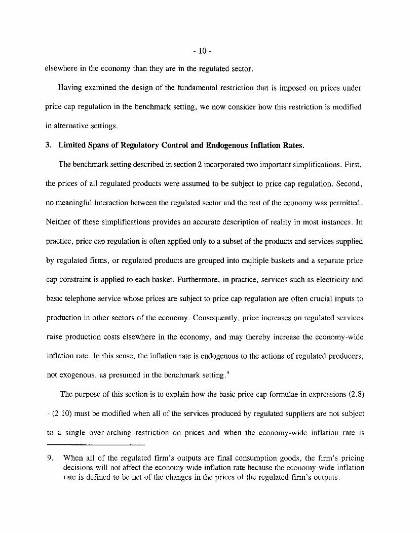
- 10-

elsewhere in the economy than they are in the regulated sector.

Having examined the design of the fundamental restriction that is imposed on prices under

price cap regulation in the benchmark setting, we now consider how this restriction is modified

in alternative settings.

3. Limited Spans of Regulatory Control and Endogenous Inflation Rates.

The benchmark setting described in section 2 incorporated two important simplifications. First,

the prices of all regulated products were assumed to be subject to price cap regulation. Second,

no meaningful interaction between the regulated sector and the rest of the economy was permitted.

Neither of these simplifications provides an accurate description of reality in most instances. In

practice, price cap regulation is often applied only to a subset of the products and services supplied

by regulated firms, or regulated products are grouped into multiple baskets and a separate price

cap constraint is applied to each basket. Furthermore, in practice, services such as electricity and

basic telephone service whose prices are subject to price cap regulation are often crucial inputs to

production in other sectors of the economy. Consequently, price increases on regulated services

raise production costs elsewhere in the economy, and may thereby increase the economy-wide

inflation rate. In this sense, the inflation rate is endogenous to the actions of regulated producers,

not exogenous, as presumed in the benchmark setting. 9

The purpose of this section is to explain how the basic price cap formulae in expressions (2.8)

- (2.10) must be modified when all of the services produced by regulated suppliers are not subject

to a single over-arching restriction on prices and when the economy-wide inflation rate is

9. When all of the regulated firm's outputs are final consumption goods, the firm's pricingdecisions will not affect the economy-wide inflation rate because the economy-wide inflationrate is defined to be net of the changes in the prices of the regulated firm's outputs.

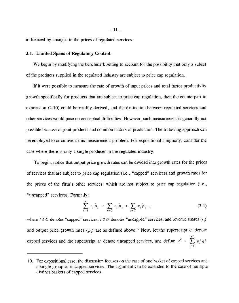
- 11 -

influenced by changes in the prices of regulated services.

3.1. Limited Spans of Regulatory Control.

We begin by modifying the benchmark setting to account for the possibility that only a subset

of the products supplied in the regulated industry are subject to price cap regulation.

If it were possible to measure the rate of growth of input prices and total factor productivity

growth specifically for products that are subject to price cap regulation, then the counterpart to

expression (2.10) could be readily derived, and the distinction between regulated services and

other services would pose no conceptual difficulties. However, such measurement is generally not

possible because of joint products and common factors of production. The following approach can

be employed to circumvent this measurement problem. For expositional simplicity, consider the

case where there is only a single producer in the regulated industry.

To begin, notice that output price growth rates can be divided into growth rates for the prices

of services that are subject to price cap regulation (Le., "capped" services) and growth rates for

the prices of the firm's other services, which are not subject to price cap regulation (i.e.,

"uncapped" services). Formally:

n

L riP; = L riP, + L riP; ,i=l i0C iEU

(3.1)

where i E C denotes "capped" services, i E U denotes "uncapped" services, and revenue shares (r)

and output price growth rates (p) are as defined above. lO Now, let the superscript C denotenO

capped services and the superscript U denote uncapped services, and define R C = L P ~ q~i = 1

10. For expositional ease, the discussion focuses on the case of one basket of capped services anda single group of uncapped services. The argument can be extended to the case of multipledistinct baskets of capped services.

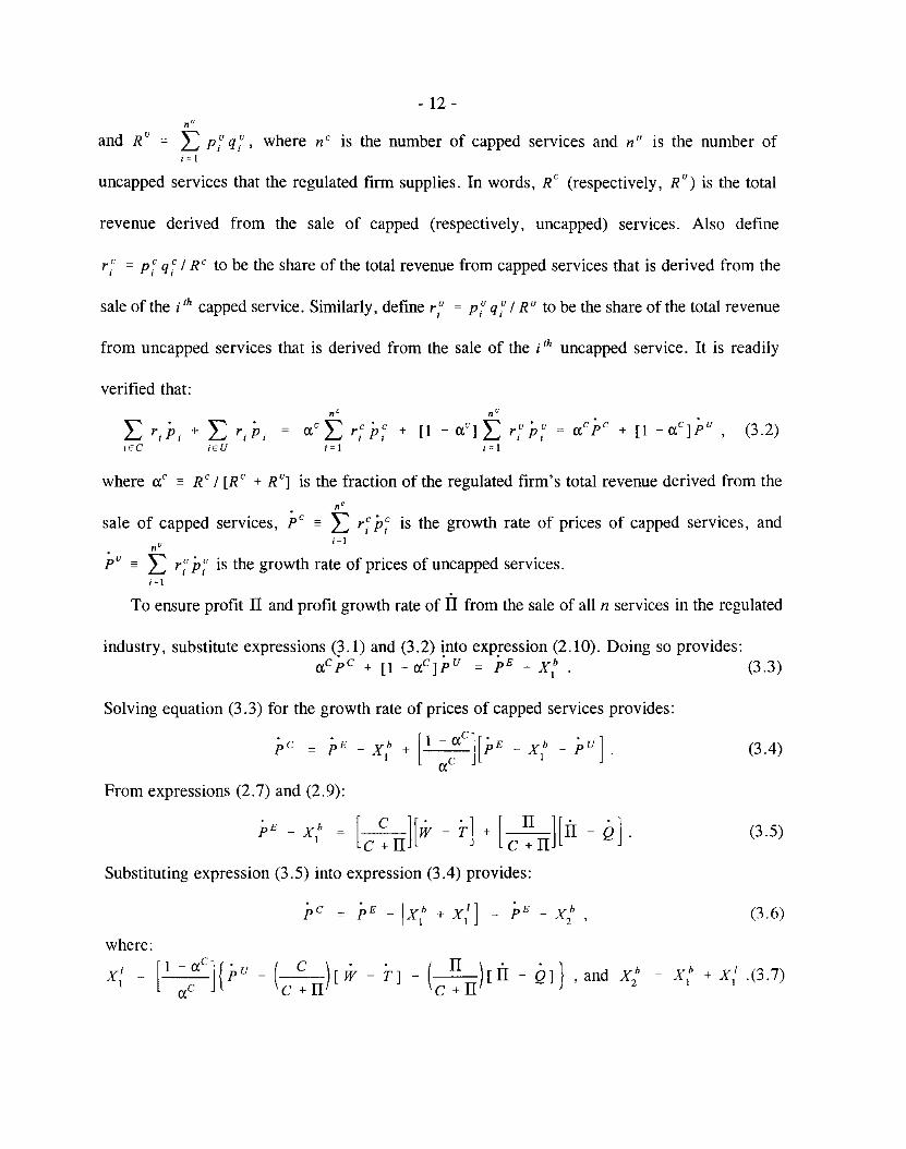
- 12 -n U

and RU

= L PiU q,U, where nC is the number of capped services and nU is the number ofi = 1

uncapped services that the regulated firm supplies. In words, RC (respectively, R

U) is the total

revenue derived from the sale of capped (respectively, uncapped) services. Also define

riC = P~ q iC

/ R C to be the share of the total revenue from capped services that is derived from the

sale of the i th capped service. Similarly, define r U = pU

qU / R U to be the share of the total revenueI I I

from uncapped services that is derived from the sale of the i th uncapped service. It is readily

verified that:n'

(lc Lr;p7j===1

n U

+ [ 1 - (XC j '" r U pU

L"(3.2)

where (XC _ R C/ [R c + RUj is the fraction of the regulated firm's total revenue derived from the

nU

pU = L r," p," is the growth rate of prices of uncapped services.i=1

n'

sale of capped services, pC = L r~ P~ is the growth rate of prices of capped services, and;=1

To ensure profit IT and profit growth rate of IT from the sale of all n services in the regulated

industry, substitute expressions (3.1) and (3.2) into expression (2.10). Doing so provides:(XC pC + [1 - (XcjPu = pE - xt . (3.3)

Solving equation (3.3) for the growth rate of prices of capped services provides:

pC = pE _xt + [1 :C(XC][pE _ Xjb _ pu].

From expressions (2.7) and (2.9):

(3.4)

(3.5)

Substituting expression (3.5) into expression (3.4) provides:

(3.6)

where:

x: = [1 -c(XC]{pu(X

- ( C ) [TV - T j - ( IT ) [11 - in} , and x;c+II c+II

xt + xi .(3.7)

(3.8)

- 13 -

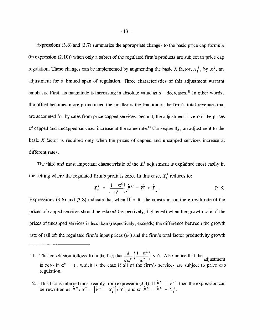
Expressions (3.6) and (3.7) summarize the appropriate changes to the basic price cap formula

(in expression (2.10)) when only a subset of the regulated firm's products are subject to price cap

regulation. These changes can be implemented by augmenting the basic X factor, X1b

, by x:' an

adjustment for a limited span of regulation. Three characteristics of this adjustment warrant

emphasis. First, its magnitude is increasing in absolute value as aC decreases. ll In other words,

the offset becomes more pronounced the smaller is the fraction of the firm's total revenues that

are accounted for by sales from price-capped services. Second, the adjustment is zero if the prices

of capped and uncapped services increase at the same rate.12 Consequently, an adjustment to the

basic X factor is required only when the prices of capped and uncapped services increase at

different rates.

The third and most important characteristic of the x: adjustment is explained most easily in

the setting where the regulated firm's profit is zero. In this case, x: reduces to:

x: = [1 :caC][pu - W+ r].Expressions (3.6) and (3.8) indicate that when IT = 0, the constraint on the growth rate of the

prices of capped services should be relaxed (respectively, tightened) when the growth rate of the

prices of uncapped services is less than (respectively, exceeds) the difference between the growth

rate of (all of) the regulated firm's input prices (w) and the firm's total factor productivity growth

11. This conclusion follows from the fact that~ ( 1 - aC

) < 0 . Also notice that the .d aC aC adjustment

is zero if aC= 1, which is the case if all of the firm's services are subject to price cap

regulation.

12. This fact is inferred most readily from expression (3.4). If Pu = pC, then the expression canbe rewritten as pC /aC= [pE ~ xt]/ aC, and so pc = pE - X 1h.

- 14 -

rate (1').[3 In other words, if the prices of uncapped services are rising less rapidly than is

necessary to ensure the regulated firm zero profit based upon its overall productivity and input

price growth rates, then the prices of capped services should be permitted to rise more rapidly than

the standard pE - X[b rate in order to allow the firm to earn zero profit overall. 14

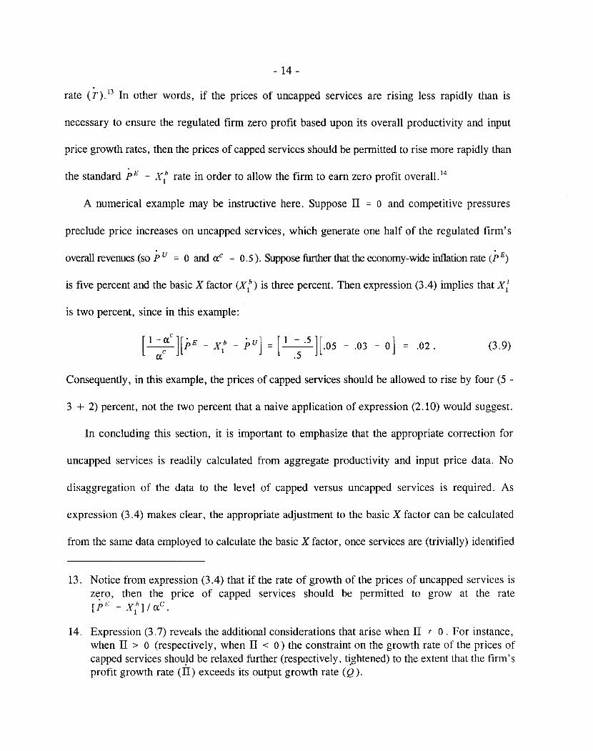
A numerical example may be instructive here. Suppose II = 0 and competitive pressures

preclude price increases on uncapped services, which generate one half of the regulated firm's

overall revenues (so Pu = 0 and (XC = 0.5). Suppose further that the economy-wide inflation rate (P E)

is five percent and the basic X factor (Xn is three percent. Then expression (3.4) implies that x:is two percent, since in this example:

(3.9)

Consequently, in this example, the prices of capped services should be allowed to rise by four (5 -

3 + 2) percent, not the two percent that a naive application of expression (2.10) would suggest.

In concluding this section, it is important to emphasize that the appropriate correction for

uncapped services is readily calculated from aggregate productivity and input price data. No

disaggregation of the data to the level of capped versus uncapped services is required. As

expression (3.4) makes clear, the appropriate adjustment to the basic X factor can be calculated

from the same data employed to calculate the basic X factor, once services are (trivially) identified

13. Notice from expression (3.4) that if the rate of growth of the prices of uncapped services iszero, then the price of capped services should be permitted to grow at the rate[pH_X[b]/(XC.

14. Expression (3.7) reveals the additional considerations that arise when II * o. For instance,when II > 0 (respectively, when II < 0) the constraint on the growth rate of the prices ofcapped services shou)d be relaxed further (respectively, t~ghtened) to the extent that the firm'sprofit growth rate (II) exceeds its output growth rate (Q).

- 15 -

as being subject to price cap regulation or not subject to price cap regulation.

3.2. Endogenous Inflation Rates.

We now modify the benchmark setting to allow for the possibility that some of the outputs of

the regulated sector are intermediate goods that other firms in the economy employ to produce

final goods. When this possibility arises, the prices established in the regulated industry can have

a direct impact on the economy-wide rate of output price inflation, as firms adjust their output

prices in response to changes in the input prices they face. When the impact of regulated prices

on the economy-wide inflation rate is pronounced, it is important to account for this impact

explicitly. It is possible to do so as follows.

To begin, divide the mE inputs employed outside of the regulated sector into the m G inputs

that are produced in the regulated sector and them N inputs that are not produced in the regulated

sector. Similarly, distinguish between the nJ outputs produced in the regulated sector that serve

as intermediate goods elsewhere in the economy and the n F regulated outputs that are final goods.

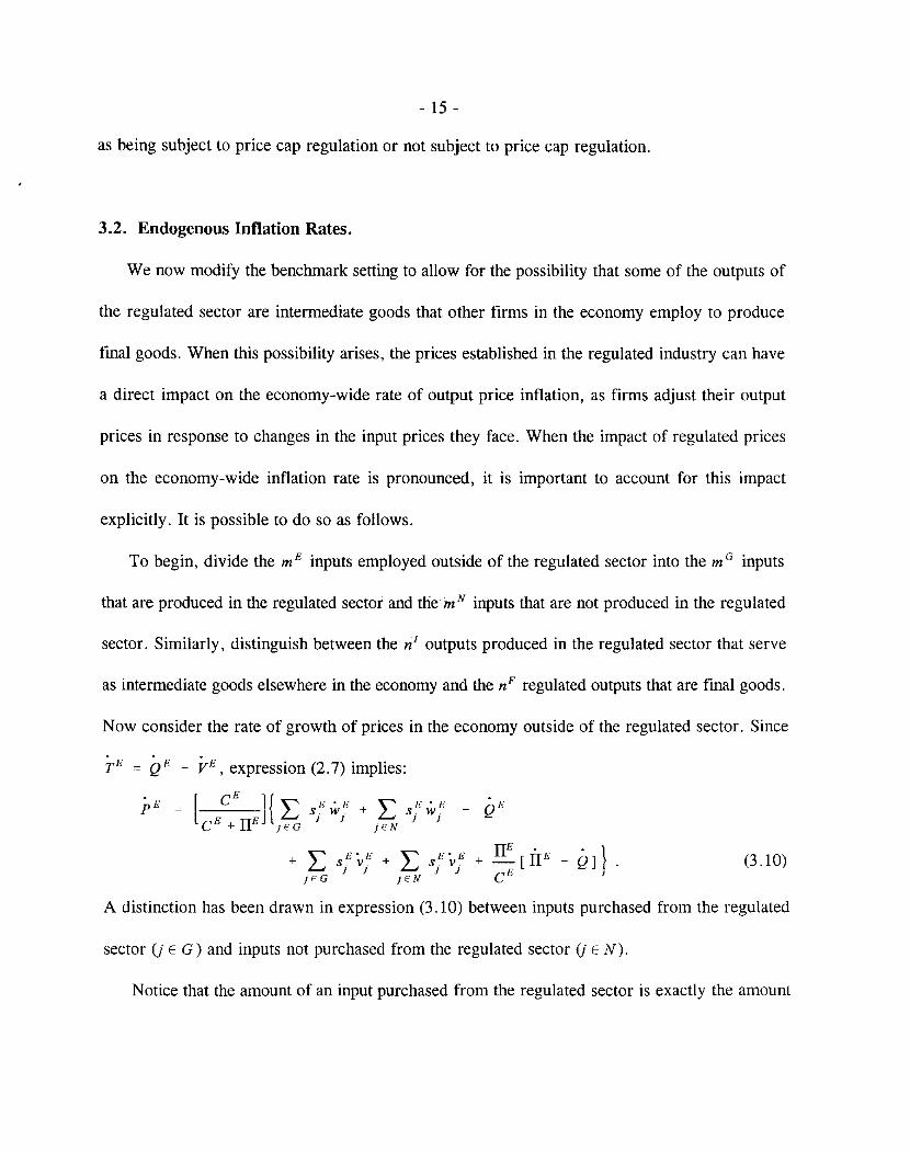
Now consider the rate of growth of prices in the economy outside of the regulated sector. Since

(3.10)

A distinction has been drawn in expression (3.10) between inputs purchased from the regulated

sector (j E G) and inputs not purchased from the regulated sector (j EN).

Notice that the amount of an input purchased from the regulated sector is exactly the amount

- 16 -

of the corresponding intermediate good produced in the regulated sector. Formally, if v G denotes1

the amount of the j rh input purchased from the regulated sector and if ql denotes the amount of1

the j th intermediate good produced in the regulated sector, then v G = qI. Similarly, the unit cost1 1

of an input purchased from the regulated sector (w G) is precisely the price of the corresponding1

intermediate output produced in the regulated sector (pI), so w G = pl. Furthermore, the total cost1 1 1

incurred in the economy from buying the inputs produced in the regulated sector (e G) is exactly

the total revenue derived in the regulated sector from the sale of intermediate goods (R I). In

addition, total input costs outside of the regulated sector (e E) are the sum of the cost of inputs

purchased from the regulated sector (e G) and the cost of inputs not purchased from the regulated

sector (eN). Similarly, total revenue in the regulated sector (R) is the sum of the regulated

revenue derived from selling intermediate goods (R I) and the regulated revenue derived from

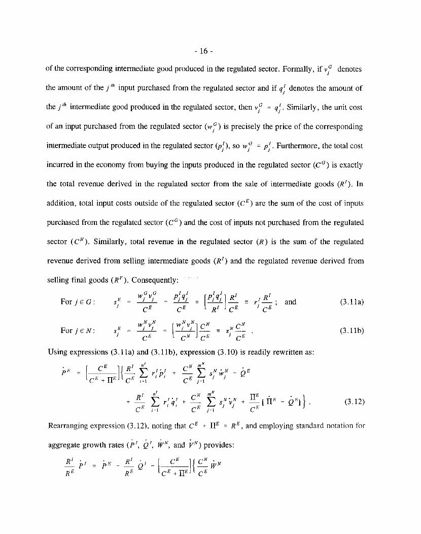
selling final goods (R F). Consequently:

For j E G:

For jEN:

wGv G plql I I IR I

E 1 1 _1_1 = [Pi qi ]!!:- r l_. ands. -1

e E e E R I e E i e E '

wNv N[WNV

N] N eN

sE = _1_1_ = _1_1_ ~ - SN_1

e E eN e E 1e E

(3.11a)

(3. 11b)

Using expressions (3. 11a) and (3.11b), expression (3.10) is readily rewritten as:

+ (3.12)

Rearranging expression (3.12), noting that e E + lIE = RE, and employing standard notation for

- 17 -

Now define:

X3h

= [(CEC+NlJE)WN- (C~II)W] + [(C~II)T - (CEC+EIIJ(QE - ~>'N)]

+[(CE~EIIJllE - (C ~II)ll] + [(C ~II)Q - (CE~EIIE)QE].

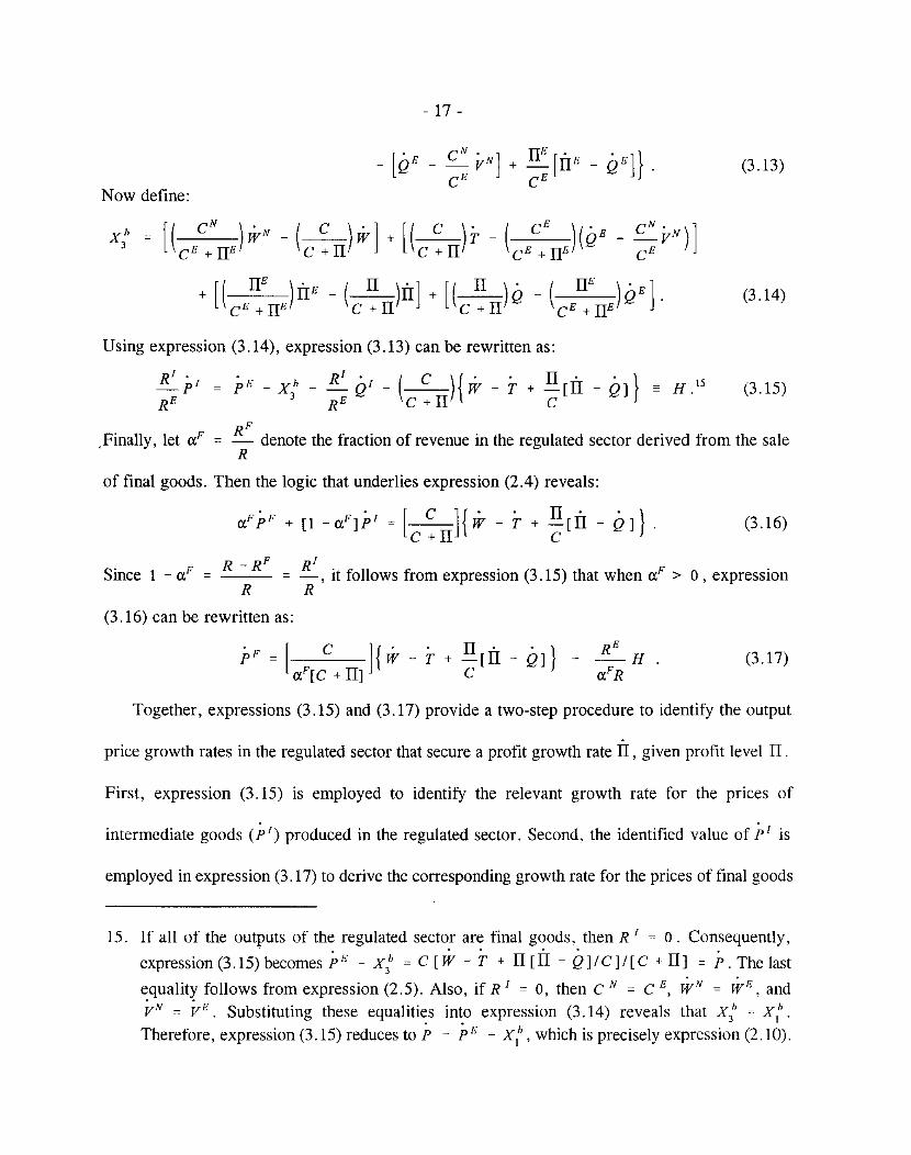
Using expression (3.14), expression (3.13) can be rewritten as:

(3.13)

(3.14)

.Finally, let a,F

pE _ x b _ j{ QI _ ( C ){w _T + II[ll - Q]} = H. 15 (3.15)3 RE C + II C

RF

denote the fraction of revenue in the regulated sector derived from the saleR

of final goods. Then the logic that underlies expression (2.4) reveals:

. . [C]{' . II' '}a,FpF + [1 _a,F]pI = -- W - T + -[II - Q] .c+II C

(3.16)

R - R F R I

Since 1 - a,F = = -, it follows from expression (3.15) that when a,F > 0, expressionR R

(3.16) can be rewritten as:

(3.17)

Together, expressions (3.15) and (3.17) provide a two-step procedure to identify the output

price growth rates in the regulated sector that secure a profit growth rate II, given profit level II.

First, expression (3.15) is employed to identify the relevant growth rate for the prices of

intermediate goods (pI) produced in the regulated sector. Second, the identified value of pI is

employed in expression (3.17) to derive the corresponding growth rate for the prices of final goods

15. If all of the outputs of the regulated sector are final goods, then R I = O. Consequently,

expression(3.15)becomespE - X3h = C[W - T + II[ll - Q]/C]/[C + II] = P. The last

equality follows from expression (2.5). Also, if RI = 0, then C N= C E, wN= WE, andvN = vE

• Substituting these equalities into expression (3.14) reveals that X 3h = x

j

h•

Therefore, expression (3.15) reduces to P = PE - xt, which is precisely expression (2.10).

[1 + ~]p = pE -X3b - ~Q. (3.18)RE RE

denote the fraction of revenue generated in both the regulated sector and

- 18 -

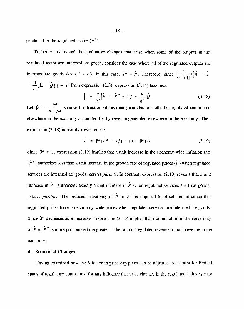
produced in the regulated sector (pF).

To better understand the qualitative changes that arise when some of the outputs in the

regulated sector are intermediate goods, consider the case where all of the regulated outputs are

intermediate goods (so R I = R). In this case, pI = P. Therefore, since ( c ){ W - Tc+II

+ II [ll - Ql} = P from expression (2.3), expression (3.15) becomes:c

RELet pE = _

R +R E

elsewhere in the economy accounted for by revenue generated elsewhere in the economy. Then

expression (3.18) is readily rewritten as:

(3.19)

Since pE < 1, expression (3.19) implies that a unit increase in the economy-wide inflation rate

(P E) authorizes less than a unit increase in the growth rate of regulated prices (P) when regulated

services are intermediate goods, ceteris paribus. In contrast, expression (2.10) reveals that a unit

increase in pE authorizes exactly a unit increase in P when regulated services are final goods,

ceteris paribus. The reduced sensitivity of P to pE is imposed to offset the influence that

regulated prices have on economy-wide prices when regulated services are intermediate goods.

Since pE decreases as R increases, expression (3.19) implies that the reduction in the sensitivity

of P to PE is more pronounced the greater is the ratio of regulated revenue to total revenue in the

economy.

4. Structural Changes.

Having examined how the X factor in price cap plans can be adjusted to account for limited

spans of regulatory control and for any influence that price changes in the regulated industry may

- 19 -

have on economy-wide inflation rates, we now examine appropriate adjustments for anticipated

structural changes in the regulated industry. A switch from rate-of-return regulation to price cap

regulation itself can constitute an important structural change, as can a significant increase in

competitive pressure in the regulated industry.

Absent structural changes in the industry, historic productivity and input price growth rates

can serve as reasonable estimates of corresponding future growth rates. Consequently, when

structural changes are absent, historic growth rates can serve as proxies for anticipated future

growth rates, and so can be substituted into expression (2.9) to derive a reasonable value for the

basic X factor that is imposed in price cap regulation plans. More generally, however, structural

changes can render inappropriate X factors that simply reflect historic growth rates.

When a new regulatory regime and/or competitive pressures can reasonably be expected to

motivate the regulated firm to enhance its realized productivity growth rate, historic growth rates

can understate the most appropriate X factor to impose on the regulated firm. To account for this

fact, the basic X factor in price cap regulation plans can be (and often is) augmented by what is

called a customer productivity dividend (CPD) or a stretch factor. 16 In principle, the CPD should

reflect the best estimate of the increase in the productivity growth rate in the regulated sector that

will be induced by the new enhanced incentives in the regulated industry.17 In practice, the choice

16. The Federal Communications Commission imposed a CPD of .5% annually in its price capplan for AT&T.

17. To the extent that stretch factors are designed to reflect the enhanced incentives that a newregulatory regime provides, it can be appropriate to implement a stretch factor that declinesin magnitude over time as the number of years that the regulatory plan is in effect increases.Also notice that a smaller stretch factor is appropriate in cases where a regulated firm hasoperated diligently before the imposition of price cap regulation, perhaps in response topressure from competitors. Thus, the magnitude of the stretch factor that is imposed in

- 20-

of CPD can be less scientific.

Although increased competitive pressures can induce the regulated firm to operate more

diligently and thereby increase its realized productivity growth rate directly, competitive pressures

can have additional indirect effects on the firm's productivity growth rate. Some of these effects

can serve to reduce the firm's productivity growth rate, thereby rendering ambiguous the net

impact of competition on the firm's productivity growth rate, particularly in the short run.

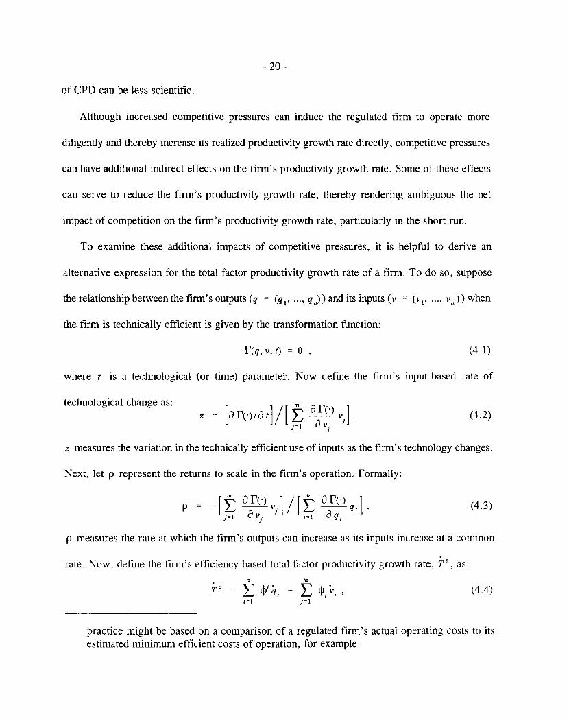
To examine these additional impacts of competitive pressures, it is helpful to derive an

alternative expression for the total factor productivity growth rate of a firm. To do so, suppose

the relationship between the firm's outputs (q = (q l' ... , qn) ) and its inputs (v = (V I' ... , vm) ) when

the firm is technically efficient is given by the transformation function:

r(q, v, t) = 0 , (4.1)

where t is a technological (or time) parameter. Now define the firm's input-based rate of

technological change as:(4.2)

z measures the variation in the technically efficient use of inputs as the firm's technology changes.

Next, let p represent the returns to scale in the firm's operation. Formally:

(4.3)

p measures the rate at which the firm's outputs can increase as its inputs increase at a common

rate. Now, define the firm's efficiency-based total factor productivity growth rate, T e, as:

n m

Te

= L q/qi - L t/JjVj ,i=t j=1

(4.4)

practice might be based on a comparison of a regulated firm's actual operating costs to itsestimated minimum efficient costs of operation, for example.

- 21 -

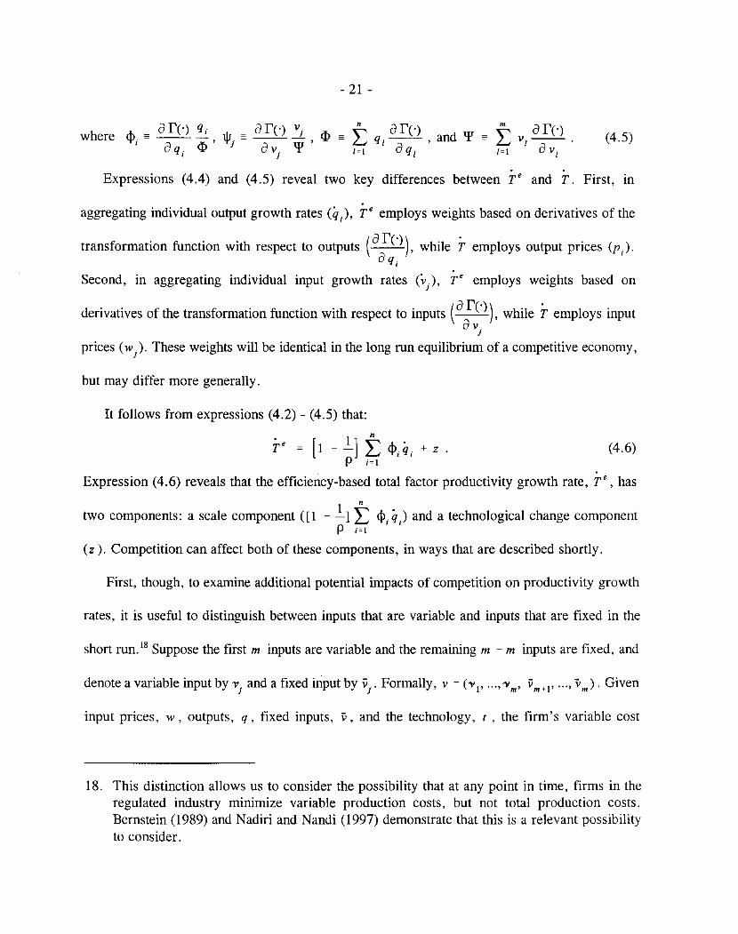
(4.5)

. .Expressions (4.4) and (4.5) reveal two key differences between T e and T. First, in

aggregating individual output growth rates (q), T e employs weights based on derivatives of the

transformation function with respect to outputs (a r(.»), while T employs output prices (p j)'aqj

Second, in aggregating individual input growth rates (v), r e employs weights based on}

derivatives of the transformation function with respect to inputs (a r(.»), while T employs inputav

}

prices (w}). These weights will be identical in the long run equilibrium of a competitive economy,

but may differ more generally.

It follows from expressions (4.2) - (4.5) that:

(4.6)

Expression (4.6) reveals that the efficiency-based total factor productivity growth rate, T e, has

two components: a scale component ([ 1 - ~1t <1\ q) and a technological change componentp ;=1

(z). Competition can affect both of these components, in ways that are described shortly.

First, though, to examine additional potential impacts of competition on productivity growth

rates, it is useful to distinguish between inputs that are variable and inputs that are fixed in the

short run. 18 Suppose the first m inputs are variable and the remaining m - m inputs are fixed, and

denote a variable input by 'Vj

and a fixed input by iii' Formally, v = (11 I' ... ,11m' iim+1' ... , iim) . Given

input prices, w, outputs, q, fixed inputs, ii, and the technology, t , the firm's variable cost

18. This distinction allows us to consider the possibility that at any point in time, firms in theregulated industry minimize variable production costs, but not total production costs.Bernstein (1989) and Nadiri and Nandi (1997) demonstrate that this is a relevant possibilityto consider.

- 22 -

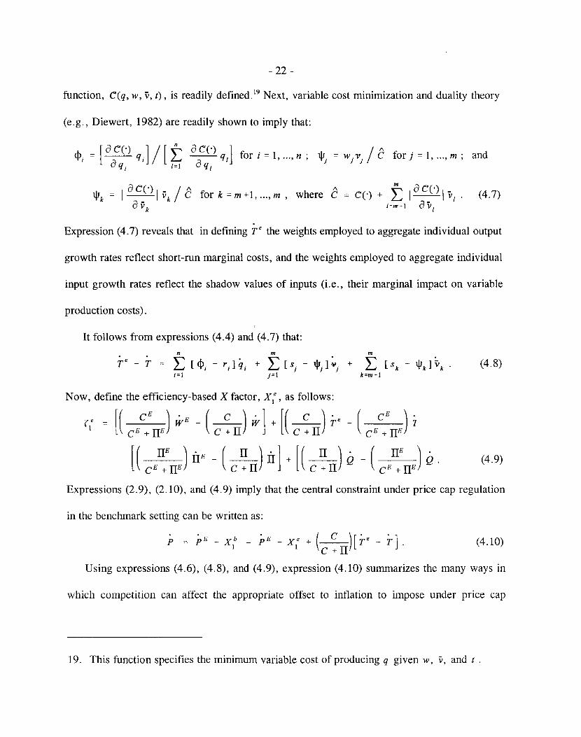
function, C(q, w, v, t), is readily defined. 19 Next, variable cost minimization and duality theory

(e.g., Diewert, 1982) are readily shown to imply that:

IJ1 = 12CO!v /8 fork=m+l, ... ,m, where 8~c(')+ t1 2CO lv l . (4.7)k 2 - k 2v k 10m'l vI

Expression (4.7) reveals that in defining Te the weights employed to aggregate individual output

growth rates reflect short-run marginal costs, and the weights employed to aggregate individual

input growth rates reflect the shadow values of inputs (i.e., their marginal impact on variable

production costs).

It follows from expressions (4.4) and (4.7) that:n m

Te- T = '" [<I> - r 1q + '" [s. - 1J11 ~ +L..., I II L...J] lJ

;01 jol

Now, define the efficiency-based X factor, xle

, as follows:

m

L [Sk - IJ1k ]Vkk=m+l

(4.8)

(4.10)

{Ie = [( cEC+ErrJ WE - (C ~rr) W] +[( C~rr) re- (cEC+ErrJ i

[( cE~ErrJ IiE - (C ~rr) Ii] +[( C~rr) Q - (cE~ErrJ Q. (4.9)

Expressions (2.9), (2.10), and (4.9) imply that the central constraint under price cap regulation

in the benchmark setting can be written as:

p = pE - X 1b

= pE - x le + (C ~ rrl[ r e- T] .

Using expressions (4.6), (4.8), and (4.9), expression (4.10) summarizes the many ways in

which competition can affect the appropriate offset to inflation to impose under price cap

19. This function specifies the minimum variable cost of producing q given w, v, and t .

- 23 -

regulation. First, competition can affect T" , and therefore xt .From expression (4.8), competitive

pressures may speed technological progress, thereby increasing T" and Xl" (by increasing z). In

contrast, as it shifts sales from an incumbent supplier to new entrants, competition can reduce the

incumbent supplier's scale economies (p), particularly in the short run when the presence of fixed

inputs limits the incumbent supplier's ability to reduce inputs at the same rate that outputs decline.

The reduction inp reduces r", and therefore XI".20 r" and XI" are also reduced to the extent that

competition reduces the output growth rates (q) of the incumbent supplier.

. .Second, competition can affect the difference between T" and T in a variety of ways, as

expression (4.8) reveals. For instance, as competitors attract customers from an incumbent

supplier, the incumbent's output growth rates (q) slow. The slow-down is often most pronounced

on services with high price-cost margins (r; - <1», since competitors typically seek to attract the

most profitable customers. This effect serves to increase T" - T (from expression (4.8», and

thus to increase the appropriate rate at which the incumbent supplier's output prices should be

permitted to rise under price cap regulation (from expression (4.10». Similarly, competition can

drive down prices and thereby reduce the profit margins (r; - <1» earned by incumbent suppliers.

If the margin reductions are particularly pronounced on services with the highest growth rates

(q), then higher output price growth rates can be appropriate for the incumbent supplier, as

expressions (4.8) and (4.10) reveal.

Additional impacts of competition on the appropriate rate of growth of output prices (P) under

price cap regulation can also be inferred from expressions (4.7) - (4.10). As just one additional

20. Recent studies suggest that a one percent decline in output growth is associated with a declinein productivity growth of approximately one half of one percent in the telecommunicationsindustry. See Crandall (1991, p. 70), and Staranczak et al. (1994), for example.

- 24-

illustration, notice that competition for scarce resources (such as skilled labor and specialized

equipment) can alter the employment and prices of these resources, and thus total production costs.

Consequently, the weights (s k and s) employed to aggregate individual input growth rates can

vary, as can the growth rates themselves. The corresponding implications for the most appropriate

value of P are reflected in expression (4.10).21

In summary, we have explained how the X factor should be adjusted, in principle, to reflect

the impact of anticipated structural changes (such as increased competition) in the regulated

industry. In practice, it is difficult to identify in advance and quantify precisely all relevant

dimensions of structural changes. But the possibility of structural changes and their implications

for the appropriate X factor merit careful thought nevertheless.

5. Conclusions.

We have reviewed the standard principles that inform the choice of an X factor in price cap

regulation plans. We have also extended the standard analysis to account for limited spans of

regulatory control, endogenous economy-wide inflation rates, and structural shifts in industry

conditions. In closing, we mention two of the many additional effects that warrant consideration

21. One other potential impact of competition warrants brief mention. If competition particularlydampens the growth rate of prices of uncapped services, then the ceiling on the growth rateof prices of capped services should be raised. This effect can be demonstrated formally byemploying the logic that underlies expressions (3.1) - (3.7). This logic reveals that when theregulated firm's services consist of capped and uncapped services, the counterpart toexpression (4.10) is:

pC = pE _ x2e + [1 :CUC][pE _X 2' _ pu]

where x; = XI' - [c ~ rrll j-' - T], and where all other notation is defined as in the text.

- 25 -

in extensions of our analysis.22

First, service quality merits careful consideration. Our analysis implicitly assumed that service

quality did not change when price cap regulation was imposed. If quality does change, then

additional modification of the X factor can be appropriate in some settings. As service quality

declines, customers generally derive less value from their consumption of regulated services,

ceteris paribus. Price reductions can be appropriate to compensate customers for the losses they

suffer. One way to implement price reductions as quality declines is to increase the X factor as

measured service quality falls. 23

Second, our analysis has focused on forward-looking estimates of productivity growth rates.

In practice, some price cap plans allow unanticipated events in the industry to trigger changes in

the X factor. For instance, the X factor might be decreased if new taxes are imposed on the

regulated firm, or if key input costs rise well beyond anticipated levels. Such changes to the X

factor can be appropriate if they do not insure the regulated firm against inappropriate activities

that it might undertake. For instance, it is generally unwise to automatically raise the authorized

X factor to account for all of the extra costs that a power producer incurs as fuel costs rise. Such

automatic adjustments reduce the firm's incentives to secure fuel at low prices and to choose the

least-cost technology for production.

22. See Mitchell and Vogelsang (1991), Kwoka (1993), Armstrong et al. (1994), and Sappingtonand Weisman (1996), among others, for some thoughts on these effects and other importantconsiderations in the design of price cap regulation.

23. Mandated rebates to customers who suffer service quality degradation are an alternativemeans of promoting high levels of service quality. Direct rebates to affected customers havethe virtue of ensuring that the effective price decrease is delivered to the customers whoexperience the decline in service quality. Increasing the X factor as service quality declinesdoes not necessarily share this virtue.

REFERENCES

Armstrong, Mark, Simon Cowan, and John Vickers, Regulatory Reform: Economic Analysis andBritish Experience. Cambridge, MA: MIT Press, 1994.

Beesley, Michael and Stephen Littlechild, "The Regulation of Privatized Monopolies in the UnitedKingdom," Rand Journal ofEconomics , 20(3), Autumn 1989, 454-472.

Bernstein, Jeffrey, "An Examination of the Equilibrium Specification and Structure of Productionfor Canadian Telecommunications," Journal ofApplied Econometrics, 4, 1989, 265-282.

Braeutigam, Ronald and John Panzar, "Diversification Incentives Under "Price-Based" and"Cost-Based" Regulation," Rand Journal ofEconomics, 20(3), Autumn 1989, 373-391.

Brennan, Timothy, "Regulating By Capping Prices", Journal ofRegulatory Economics, 1(2), June1989, 133-147.

Cabral, Luis and Michael Riordan, "Incentives for Cost Reduction Under Price Cap Regulation",Journal ofRegulatory Economics, 1(2), June 1989, 93-102.

Crandall, Robert, After the Breakup: U.S. Telecommunications in a More Competitive Era.Washington, D.C.: Brookings Institution, 1991.

Diewert, W. Erwin, "Duality Approaches to Microeconomic Theory," in K. Arrow and M.Intriligator (eds.), Handbook of Mathematical Economics. New York: Elsevier SciencePublishers, 1982, Volume II, pp. 535-599.

Diewert, W. Erwin, "Index Number Issues in Incentive Regulation," University of BritishColumbia Discussion Paper No. 93-06, January 1993.

Kirchhoff, Herb, "Earnings Regulation for Big Incumbent Telcos Just About Extinct in EasternU.S.," State Telephone Regulation Report, 16(7), April 3, 1998a, 1-4.

Kirchhoff, Herb, "Price Caps Still Struggle in Western States, But '98 May See Some Changes,"State Telephone Regulation Report, 16(8), April 17, 1998b, 1-2.

Kwoka, John, "Productivity and Price Caps in Telecommunications ," in Michael Einhorn (ed.),Price Caps and Incentive Regulation in Telecommunications. Boston: Kluwer AcademicPublishers, 1990, pp. 77-93.

Kwoka, John, "Implementing Price Caps in Telecommunications," Journal of Policy Analysis andManagement, 12(4), 1993,726-752.

Lewis, Tracy and David Sappington, "Regulatory Options and Price Cap Regulation," RandJournal ofEconomics , 20(3), Autumn 1989,405-416.

- R2 -

Mitchell, Bridger and Ingo Vogelsang, Telecommunications Pricing: Theory and Practice.Cambridge: Cambridge University Press, 1991.

Morten Dalen, Dag, "Yardstick Competition and Investment Incentives," Journal ofEconomicsand Management Strategy, 7(1), Spring 1998, 105-126.

Nadiri, M. Ishaq and Banani Nandi, "The Changing Structure of Cost and Demand for the U.S.Telecommunications Industry," Information Economics and Policy, 9(4), December 1997,319-347.

Pint, Ellen, "Price-Cap Versus Rate-of-Return Regulation in a Stochastic-Cost Model", RandJournal ofEconomics, 23(4), Winter 1992,564-578.

Sappington, David and Dennis Weisman, Designing Incentive Regulation for theTelecommunications Industry. Cambridge, MA: MIT Press, 1996.

Schmalensee, Richard, "Good Regulatory Regimes," Rand Journal ofEconomics, 20(3), Autumn1989,417-436.

Shleifer, Andrei, "A Theory of Yardstick Competition," Rand Journal of Economics, 16(3),Autumn 1985, 319-327.

Sobel, Joel, "A Re-examination of Yardstick Competition," University of California- San Diegomimeo, October 1997.

Staranczak, Genio, Edgardo Sepulveda, Peter Dilworth, and Shaft Shaikh, "Industry Structure,Productivity, and International Competitiveness: The Case of Telecommunications,"Information Economics and Policy, 6(2), July 1994, 121-142.