
Monte Carlo methods forintegro-differential equations
Lecture 2: Kinetic equations
Lorenzo Pareschi
Department of Mathematics & CMCSUniversity of Ferrara
Italy
http://utenti.unife.it/lorenzo.pareschi/[email protected]
NSPDE2Malaga, February 8-12, 2010
Lorenzo Pareschi (Univ. Ferrara) MC methods for integro-differential equations #2 Malaga, February 8-12, 2010 1 / 63

Course Outline
1 Lecture #1: Monte Carlo methods(a) Introduction to Monte Carlo methods(b) Integration and applications to PDEs
2 Lecture #2: Kinetic equations(a) Direct Simulation Monte Carlo(b) Asymptotic Preserving Monte Carlo
Lorenzo Pareschi (Univ. Ferrara) MC methods for integro-differential equations #2 Malaga, February 8-12, 2010 2 / 63

Outline
1 IntroductionLevels of representationThe Boltzmann equationHydrodynamic limitsSplitting approach
2 Direct Simulation Monte Carlo methodsDSMC methodsNanbu’s methodNanbu-Babovsky methodBird’s methodFinal remarks
3 Asymptotic Preserving Monte Carlo methodsExponential methodsMonte Carlo methodsNumerical resultsFurther developments
Lorenzo Pareschi (Univ. Ferrara) MC methods for integro-differential equations #2 Malaga, February 8-12, 2010 3 / 63
Introduction
Introduction
Finally let us consider more generally the group of problems which gave
rise to the development of the method to which this article is
devoted.. . . The problem of the behavior of such a system is formulated
by a set of integro-differential equations. Such equations are known in
the kinetic theory of gases as the Boltzmann equation. In the theory of
probability one has a somewhat similar situation described by the
Fokker-Planck equation.
(N.Metropilis, S.Ulam, ”The Monte Carlo method”, J. Am. Stat. Ass., 1949.)
Lorenzo Pareschi (Univ. Ferrara) MC methods for integro-differential equations #2 Malaga, February 8-12, 2010 4 / 63

Introduction Levels of representation
Levels of representation
Interacting particle systems are ubiquitous in nature: gases, fluids, plasmas,solids (metals, semiconductors or insulators), vehicles on a road, economicagents can be considered as interacting particle systems.
Particle systems can be described at the microscopic level by particledynamics (Newton’s equations) describing the individual motions of theparticles. However, particle dynamic is impossible to use in most practicalcases, due to the extraordinary large number of equations that must besolved simultaneously.
At the macroscopic level fluid models (such as the Euler or Navier-Stokes
equations) describe averaged quantities, local density, momentum, energy...However, fluid models involve constants (viscosity, heat conductivity,diffusion) which depend on the microscopic properties of the elementaryparticles interactions.
Lorenzo Pareschi (Univ. Ferrara) MC methods for integro-differential equations #2 Malaga, February 8-12, 2010 6 / 63

Introduction Levels of representation
There is a need to bridge the gap between particle dynamics and fluidmodels. This question of how to pass from microscopic properties of mattersto macroscopic properties of systems is one of the most fundamental ones inphysics. It is also one of the most difficult.
The problem is slightly simplified by introducing an intermediate stepbetween particle systems and fluid models: the so-called kinetic level. Thesemodels, characterized by Boltzmann equations, deal with a quantity, thedistribution function, which is the density of particles in phase-space (sayposition and velocity).
The essential idea of Monte Carlo or particle simulations for the Boltzmannequation is to return to the particle description with a number of particlessmall enough to make the situation computationally treatable but”sufficiently close” to the physical situation. As we will see this will involveevaluations of high dimensional integrals for which Monte Carlo methodsarise quite naturally.
Lorenzo Pareschi (Univ. Ferrara) MC methods for integro-differential equations #2 Malaga, February 8-12, 2010 7 / 63

Introduction Levels of representation
Microscopic, kinetic and computational levels
Microscopic level N≈ 1023
Kinetic level Boltzmann equation
Monte Carlo simulation N≈ 105
Directmethod
Consistentmethod
N→∞, δ→ 0, Nδ2=κBoltzmann−Grad limit
Applications
Lorenzo Pareschi (Univ. Ferrara) MC methods for integro-differential equations #2 Malaga, February 8-12, 2010 8 / 63

Introduction The Boltzmann equation
The kinetic modelIn the Boltzmann description of rarefied gas dynamics, the density f = f(x, v, t)of particles follows the equation
∂f
∂t+ v · ∇xf =
1
εQ(f, f), x ∈ Ω ⊂ IR3, v ∈ IR3,
The parameter ε > 0 is called Knudsen number and it is proportional to the meanfree path between collisions. The bilinear collision operator Q(f, f) is given by
Q(f, f)(v) =
∫
IR3
∫
S2
B(f(v′)f(v′
∗) − f(v)f(v∗))dv∗dσ,
where σ is a vector of the unitary sphere S2 ⊂ IR3 and the dependence of f on xand t has been omitted.The kernel B characterizes the binary interactions. TheVariable Hard Spheres1 (VHS) model used for RGD simulations is
B(|q|, |q · σ|) = C|q|α, 0 ≤ α ≤ 1,
where C is a positive constant. The case α = 0 corresponds to a Maxwellian gas,while α = 1 is called a Hard Sphere Gas.
1G.Bird, 1976Lorenzo Pareschi (Univ. Ferrara) MC methods for integro-differential equations #2 Malaga, February 8-12, 2010 10 / 63

Introduction The Boltzmann equation
The collision sphere
v v*
v’*
v’
v−v*
|v−v
*|ω
The collisional velocities (v′, v′
∗) are associated to the velocities (v, v∗) and to the
parameter σ by the relations
v′ =1
2(v + v∗ + |q|σ), v′
∗=
1
2(v + v∗ + |q|σ),
where q = v − v∗ is the relative velocity.Lorenzo Pareschi (Univ. Ferrara) MC methods for integro-differential equations #2 Malaga, February 8-12, 2010 11 / 63

Introduction The Boltzmann equation
Main propertiesThe collision operator preserves mass, momentum and energy
∫
R3
Q(f, f)φ(v) dv = 0, φ(v) = 1, vx, vy, vz, |v|2,
and in addition is such that the H-Theorem holds∫
IR3
Q(f, f) log(f)dv ≤ 0.
This condition implies that each function f in equilibrium (i.e. Q(f, f) = 0) haslocally the form of a Maxwellian distribution
M(ρ, u, T )(v) =ρ
(2πT )3/2exp
(
−|u − v|22T
)
,
where ρ, u, T are the density, the mean velocity and the gas temperature
ρ =
∫
IR3
fdv, ρu =
∫
IR3
fvdv, T =1
3ρ
∫
IR3
(v − u)2fdv.
Lorenzo Pareschi (Univ. Ferrara) MC methods for integro-differential equations #2 Malaga, February 8-12, 2010 12 / 63

Introduction Hydrodynamic limits
Fluid limitThe most natural method to derive fluid equations is the moment method. Let usmultiply the Boltzmann equation by its collision invariants and integrate
∂
∂t
∫
R3
fφ(v) dv + ∇x
(∫
R3
vfφ(v) dv
)
= 0, φ(v) = 1, v1, v2, v3, |v|2.
These equations descrive the balance of mass, momentum and energy. Thesystem is not closed since it involves higher order moments of f .As ε → 0 we have formally Q(f, f) → 0 and thus f → M . Higher order momentsof f can be computed as function of ρ, u, and T and we obtain the compressibleEuler equations
∂ρ
∂t+ ∇x · (ρu) = 0
∂ρu
∂t+ ∇x · (ρu ⊗ u + p) = 0
∂E
∂t+ ∇x · (Eu + pu) = 0, p = ρT =
2
3E − 1
3ρu2.
Lorenzo Pareschi (Univ. Ferrara) MC methods for integro-differential equations #2 Malaga, February 8-12, 2010 14 / 63

Introduction Splitting approach
Splitting approachA common approach to solve a kinetic equation is operator splitting. The solutionin one time step ∆t may be obtained by the sequence of two steps.First integrate the space homogeneous equation for all x ∈ Ω,
∂f
∂t=
1
εQ(f , f),
f(x, v, 0) = f0(x, v),
for a time step ∆t (collision step) to obtain f = C∆t(f0).Then solve the transport equation using the output of the previous step as initialcondition,
∂f
∂t+ v · ∇xf = 0,
f(x, v, 0) = f(x, v,∆t).
for a time step ∆t (transport step) to get f = T∆t(f) = T∆t(C∆t(f0)).After this splitting the major numerical difficulties are in the collision step. Notethat the transport step corresponds to simple free flow of particles.
Lorenzo Pareschi (Univ. Ferrara) MC methods for integro-differential equations #2 Malaga, February 8-12, 2010 16 / 63

Introduction Splitting approach
Splitting approachThe splitting scheme described above is first order accurate in time. Theaccuracy in time may be improved by a more sophisticated splitting. Forexample Strang splitting2 is second order accurate (provided both steps are atleast second order). It can be written as
f = C∆t/2(T∆t(C∆t/2(f0))),
or equivalently asf = T∆t/2(C∆t(T∆t/2(f0))).
Note that, if the initial data is in local equilibrium and both steps are solvedexactly, then simple splitting and Strang splitting does not differ. So simplesplitting becomes second order accurate.
Both splitting methods for vanishingly small values of ε becomes a first orderkinetic scheme for the underlying fluid dynamic limit. The collision stepbecomes a projection towards the local Maxwellian C∆t(f0) = M(f0) whichis then transported by the transport step f = T∆t(M(f0)). Thus Strangsplitting reduces its accuracy to first order in time in this regime.
2G.Strang, 1968Lorenzo Pareschi (Univ. Ferrara) MC methods for integro-differential equations #2 Malaga, February 8-12, 2010 17 / 63

Direct Simulation Monte Carlo methods DSMC methods
DSMC basicsExample: Flow past a sphere
Initialize system with particles (xi, vi), i = 1, . . . , N (sampling).Loop over time steps of size ∆t.Create particles at open boundaries.Move all the particles xi = xi + vi∆t (transport step).Process any interactions of particle and boundaries (Maxwell’s b.c.).Sort particles into cells.Select and execute random collisions (collision step).Compute average statistical values.
Lorenzo Pareschi (Univ. Ferrara) MC methods for integro-differential equations #2 Malaga, February 8-12, 2010 19 / 63

Direct Simulation Monte Carlo methods DSMC methods
DSMC for the collision step
In this paragraph we will describe the classical DSMC methods due to Bird andNanbu in the case of spatially homogeneous Boltzmann equations3.We assume that the kinetic equations can be written in the form
∂f
∂t=
1
ε[P (f, f) − µf ],
where µ > 0 is a constant and P (f, f) is a non negative bilinear operator s.t.
1
µ
∫
R
P (f, f)(v)φ(v) dv =
∫
R
f(v)φ(v) dv, φ(v) = 1, v, v2.
For the Boltzmann equation in the Maxwellian case
P (f, f) = Q+(f, f)(v) =
∫
R3
∫
S2
f(v′)f(v′
∗) dω dv∗,
and µ = 4πρ. The case of general VHS kernels will be discussed later.
3G.Bird ’63, K.Nanbu ’83Lorenzo Pareschi (Univ. Ferrara) MC methods for integro-differential equations #2 Malaga, February 8-12, 2010 20 / 63

Direct Simulation Monte Carlo methods Nanbu’s method
Nanbu’s method (DSMC no time counter)
We assume that f is a probability density, i.e. ρ =∫ +∞
−∞f(v, t) dv = 1.
Consider a time interval [0, tmax], and discretize it in ntot intervals of size ∆t.Let fn(v) be an approximation of f(v, n∆t). The forward Euler scheme writes
fn+1 =
(
1 − µ∆t
ǫ
)
fn +µ∆t
ǫ
P (fn, fn)
µ.
Clearly if fn is a probability density both P (fn, fn)/µ and fn+1 are probabilitydensities. Thus the equation has the following probabilistic interpretation.
Physical level: a particle with velocity vi will not collide with probability(1 − µ∆t/ǫ), and it will collide with probability µ∆t/ǫ, according to thecollision law described by P (fn, fn)(v).
Monte Carlo level: to sample vi from fn+1 with probability (1 − µ∆t/ǫ) wesample from fn, and with probability µ∆t/ǫ we sample from P (fn, fn)(v)/µ.
Note that ∆t ≤ ǫ/µ to have the probabilistic interpretation.
Lorenzo Pareschi (Univ. Ferrara) MC methods for integro-differential equations #2 Malaga, February 8-12, 2010 22 / 63

Direct Simulation Monte Carlo methods Nanbu’s method
Maxwellian caseFirst we consider the case where the collision kernel does not depend on therelative velocity.
Algorithm[Nanbu for Maxwell molecules]:
1. compute the initial velocity of the particles, v0i , i = 1, . . . , N,
by sampling them from the initial density f0(v)2. for n = 1 to ntot
for i = 1 to Nwith probability 1 − µ∆t/ǫ
set vn+1
i = vni
with probability µ∆t/ǫ select a random particle j compute v′
i by performing the collision
between particle i and particle j assign vn+1
i = v′
i
end for
end for
Nanbu’s algorithm is not conservative, i.e. momentum and energy are conservedonly in the mean, but not at each collision. A conservative algorithm is obtainedselecting independent particle pairs, instead of single particles.
Lorenzo Pareschi (Univ. Ferrara) MC methods for integro-differential equations #2 Malaga, February 8-12, 2010 23 / 63

Direct Simulation Monte Carlo methods Nanbu-Babovsky method
Nanbu-Babovsky for the Maxwellian caseThe expected number of collision pairs in a time step ∆t is Nµ∆t/(2ǫ).
Algorithm[Nanbu-Babovsky for Maxwell molecules]:
1. compute the initial velocity of the particles, v0i , i = 1, . . . , N,
by sampling them from the initial density f0(v)2. for n = 1 to ntot
given vni , i = 1, . . . , N
set Nc = Iround(µN∆t/(2ǫ)) select Nc pairs (i, j) uniformly among all possible pairs,
and for those
- perform the collision between i and j, and compute
v′
i and v′
j according to the collision law
- set vn+1
i = v′
i, vn+1
j = v′
j
set vn+1
i = vni for all the particles that have not been selected
end for
Here by Iround(x) we denote
Iround(x) =
⌊x⌋ + 1 with probability x − ⌊x⌋⌊x⌋ with probability ⌊x⌋ + 1 − x
where ⌊x⌋ denotes the integer part of x.Lorenzo Pareschi (Univ. Ferrara) MC methods for integro-differential equations #2 Malaga, February 8-12, 2010 25 / 63

Direct Simulation Monte Carlo methods Nanbu-Babovsky method
Collisional velocities
The collisional velocities are
v′
i =vi + vj
2+
|vi − vj |2
ω, v′
j =vi + vj
2− |vi − vj |
2ω,
where ω is chosen uniformly in the unit sphere.More precisely we have:Two-dimension:
ω =
(
cos θsin θ
)
, θ = 2πξ,
Three-dimension:
ω =
cos φ sin θsin φ sin θ
cos θ
, θ = arccos(2ξ1 − 1), φ = 2πξ2,
where ξ1, ξ2 are uniformly distributed random variables in [0, 1].
Lorenzo Pareschi (Univ. Ferrara) MC methods for integro-differential equations #2 Malaga, February 8-12, 2010 26 / 63

Direct Simulation Monte Carlo methods Nanbu-Babovsky method
Variable Hard Sphere caseThe extend the algorithm to non constant scattering cross section we shall assumethat the collision kernel satisfies some cut-off hypothesis.We will denote by QΣ(f, f) the collision operator with kernel
BΣ(|v − v∗|) = min B(|v − v∗|),Σ , Σ > 0.
and, for a fixed Σ, consider the homogeneous problem
∂f
∂t=
1
εQΣ(f, f).
The operator QΣ(f, f) can be written in the form P (f, f) − µf taking
P (f, f) = Q+Σ(f, f) + f(v)
∫
R3
∫
S2
[Σ − BΣ(|v − v∗|)]f(v∗) dω dv∗,
with µ = 4πΣρ and
Q+Σ(f, f) =
∫
R3
∫
S2
BΣ(|v − v∗|)f(v′)f(v′
∗) dω dv∗.
In this case, a simple scheme is obtained by using the acceptance-rejectiontechnique to sample the collisional velocity according to P (f, f)/µ.
Lorenzo Pareschi (Univ. Ferrara) MC methods for integro-differential equations #2 Malaga, February 8-12, 2010 27 / 63

Direct Simulation Monte Carlo methods Nanbu-Babovsky method
Nanbu-Babovsky for VHS
The conservative DSMC algorithm for VHS collision kernels can be written as
Algorithm[Nanbu-Babovsky for VHS molecules]:
1. compute the initial velocity of the particles, v0i , i = 1, . . . , N,
by sampling them from the initial density f0(v)2. for n = 1 to ntot
given vni , i = 1, . . . , N
compute an upper bound Σ of the cross section
set Nc = Iround(NρΣ∆t/(2ǫ)) select Nc dummy collision pairs (i, j) uniformly
among all possible pairs, and for those
- compute the relative cross section Bij = B(|vi − vj |)- if Σ Rand < Bij
perform the collision between i and j, and compute
v′
i and v′
j according to the collisional law
set vn+1
i = v′
i, vn+1
j = v′
j
set vn+1
i = vni for all the particles that have not collided
end for
Lorenzo Pareschi (Univ. Ferrara) MC methods for integro-differential equations #2 Malaga, February 8-12, 2010 28 / 63

Direct Simulation Monte Carlo methods Nanbu-Babovsky method
Evaluation of Σ
The upper bound Σ should be chosen as small as possible, to avoid inefficientrejection, and it should be computed fast. It is be too expensive to compute Σ as
Σ = Bmax ≡ maxij
B(|vi − vj |),
since this computation would require an O(N2) operations.An upper bound of Bmax is obtained by taking Σ = B(2∆v), where
∆v = maxi
|vi − v|, v :=1
N
∑
i
vi.
Remarks:
The probabilistic interpretation breaks down if ∆t/ǫ is too large. This impliesthat the time step becomes extremely small when approaching the fluiddynamic limit.
The cost of the method is proportional to the number of dummy collisionpairs, that is µN∆t/2. Thus for a fixed final time T the total cost isindependent of the choice of ∆t = T/n. However this is true only if we donot had to compute Σ (like in the Maxwellian case).
Lorenzo Pareschi (Univ. Ferrara) MC methods for integro-differential equations #2 Malaga, February 8-12, 2010 29 / 63

Direct Simulation Monte Carlo methods Bird’s method
Bird’s method (DSMC time counter)
The method is currently the most popular method for the numerical solution ofthe Boltzmann equation. It has been derived accordingly to physical considerations(as a simplified molecular dynamics) for the simulation of particle collisions.Let us consider first the Maxwellian case. The number of collisions in a short timestep ∆t is given by
Nc =Nµ∆t
2ε, µ = 4πρ.
This means that the average time between collisions ∆tc is given by
∆tc =∆t
Nc=
2ε
µN.
The method is then based on selecting randomly a particle pair, compute thecollision result and update the local time counter by ∆tc.
Lorenzo Pareschi (Univ. Ferrara) MC methods for integro-differential equations #2 Malaga, February 8-12, 2010 31 / 63

Direct Simulation Monte Carlo methods Bird’s method
Bird for Maxwellian caseIt is possible to set a time counter, tc, and to perform the calculation as follows
Algorithm[Bird for Maxwell molecules]:
1. compute the initial velocity of the particles, v0i , i = 1, . . . , N,
by sampling them from the initial density f0(v)2. set time counter tc = 03. set ∆tc = 2ε/(µN)4. for n = 1 to ntot
repeat
- select a random pair (i, j) uniformly within all possible pairs
- perform the collision and produce v′
i, v′
j
- set vi = v′
i, vj = v′
j
- update the time counter tc = tc − ∆tc
until tc ≥ (n + 1)∆t set vn+1
i = vi, i = 1, . . . , Nend for
The algorithm is similar to the Nanbu-Babovsky (NB) scheme for Maxwellianmolecules. The main difference is that in NB scheme the particles can collide onlyonce per time step, while in Bird’s scheme multiple collisions are allowed.
Lorenzo Pareschi (Univ. Ferrara) MC methods for integro-differential equations #2 Malaga, February 8-12, 2010 32 / 63

Direct Simulation Monte Carlo methods Bird’s method
Variable Hard Sphere caseFor a more general kernel, Bird’s scheme is modified to take into account that theaverage number of collisions in a given time interval is not constant, and that thecollision probability on all pairs is not uniform. This can be done as follows.The expected number of collisions in a time step ∆t is given by
Nc =NρB∆t
2ε,
where B denotes the average collision frequency.Then the mean collision time can be computed as
∆tc =∆t
Nc=
2ε
NρB.
The Nc collisions have to be performed with probability proportional toBij = B(|vi − vj |). In order to do this one can use the same acceptance-rejectiontechnique as in Nanbu-Babovsky scheme. The drawback of this procedure is thatcomputing B is too expensive. To avoid this one computes a local time counter asfollows. First select a collision pair (i, j) using rejection. Then compute
∆tij =2ε
NρBij.
Lorenzo Pareschi (Univ. Ferrara) MC methods for integro-differential equations #2 Malaga, February 8-12, 2010 33 / 63

Direct Simulation Monte Carlo methods Bird’s method
Bird for VHSBird’s algorithm for general VHS molecules can therefore be summarized as:
Algorithm[Bird for VHS molecules]:
1. compute the initial velocity of the particles, v0i , i = 1, . . . , N,
by sampling them from the initial density f0(v)2. set time counter tc = 03. for n = 1 to ntot
compute an upper bound Σ of the cross section
repeat
- select a random pair (i, j) uniformly
- compute the relative cross section Bij = B(|vi − vj |)- if Σ ξ < Bij
• perform the collision between i and j, and compute
v′
i and v′
j according to the collisional law
• set vi = v′
i, vj = v′
j
• set ∆tij = 2ε/(NρBij)• update the time counter tc = tc + ∆tij
until tc ≥ (n + 1)∆t set vn+1
i = vi, i = 1, . . . , Nend for
Lorenzo Pareschi (Univ. Ferrara) MC methods for integro-differential equations #2 Malaga, February 8-12, 2010 34 / 63

Direct Simulation Monte Carlo methods Final remarks
Final remarksThe presence of multiple collisions per time step in Bird’s method has aprofound influence on the time accuracy. While Nanbu scheme converges inprobability to the time discrete Boltzmann equation, Bird’s method convergesto the space homogeneous Boltzmann equation4.
Numerical tests confirm that in space non homogeneous situations Bird’smethod with simple splitting can achieve second order accuracy in timewhereas Nanbu’s is always first order5.
In the original nonconservative form one can show that Nanbu’s method givesthe wrong expectation for the temperature6.
Exact conservation of moments forces the velocity domain to remainbounded during relaxation |vi| ≤
√2EN . As a consequence steady state
particles are never ”true” Maxwellian samples.
Similarly to Nanbu’s method also Bird’s method becomes very expensive andpractically unusable near the fluid regime. Infact, the collision time betweenthe particles ∆tij becomes very small, and a huge number of collisions isneeded in order to reach a fixed final time tmax.
4R.Illner, H.Babovski ’89, W.Wagner ’925A.Garcia, W.Wagner ’006C.Greengard, L.G.Reyna ’91Lorenzo Pareschi (Univ. Ferrara) MC methods for integro-differential equations #2 Malaga, February 8-12, 2010 36 / 63

Asymptotic Preserving Monte Carlo methods
Main goal
The goal is to construct simple and efficient Monte Carlo methods for the solutionof RGD problems in regions with a large variation in the mean free path.As a consequence the methods should have the following features
for large Knudsen numbers, the methods behave as classical DSMC methods;
for intermediate Knudsen numbers the methods are capable to speed up thecomputation time without degradation of accuracy;
in the limit of the very small Knudsen number, the collision step replaces thedistribution function by a local Maxwellian with the same moments. Themethods will behave as a stochastic kinetic scheme for the underlying Eulerequations of gas dynamics (asymptotic preserving (AP) property);
mass, momentum, and energy are preserved.
Lorenzo Pareschi (Univ. Ferrara) MC methods for integro-differential equations #2 Malaga, February 8-12, 2010 37 / 63

Asymptotic Preserving Monte Carlo methods Exponential methods
Exponential methods
Let us rewrite the homogeneous equation in the form7
∂tf =1
ε(P (f, f) − µf) =
µ
ε
(
P (f, f)
µ− M
)
+µ
ε(M − f).
Note that the above system is is composed by a linear part µ(M − f)/ε whichcharacterizes the asymptotic behavior of f and a nonlinear part(P (f, f)/µ − M)/ε which describes the deviations of P (f, f)/µ from M , orequivalently the deviations of the Boltzmann operator from the BGK model.The system has the general structure
y′ = G(y) + λ(E − y), y(t0) = y0,
where λ > 0, and E is a local equilibrium value.
7F.Filbet, S.Jin ’09, G.Dimarco, L.Pareschi ’09Lorenzo Pareschi (Univ. Ferrara) MC methods for integro-differential equations #2 Malaga, February 8-12, 2010 39 / 63

Asymptotic Preserving Monte Carlo methods Exponential methods
Exponential Runge-Kutta
We can apply an explicit exponential Runge-Kutta method to the above system inthe form 8
Y (i) = eciλ∆tyn + (1 − eciλ∆t)En + ∆t
i−1∑
j=1
Aij(λ∆t)G(Y (j)), i = 1, . . . , ν
yn+1 = eλ∆tyn + (1 − eλ∆t)En + ∆t
ν∑
i=1
Wi(λ∆t)G(Y (i)),
where ci ≥ 0, and the coefficients Aij and the weights Wi are such that
Aij(0) = aij , Wi(0) = wi, i, j = 1, . . . , ν
with aij and wi given by a standard explicit Runge-Kutta method called theunderlying method. So when G = 0 the method is exact and when λ = 0 themethod reduces to an explicit one-step method for ODEs.
8M.Hochbruck, C.Lubich, H.Selhofer ’98. S.Maset, M.Zennaro ’09Lorenzo Pareschi (Univ. Ferrara) MC methods for integro-differential equations #2 Malaga, February 8-12, 2010 40 / 63
Asymptotic Preserving Monte Carlo methods Exponential methods
IF and ETD methods
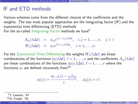
Various schemes come from the different choices of the coefficients and theweights. The two most popular approaches are the integrating factor (IF) and theexponential time differencing (ETD) methods.For the so-called Integrating Factor methods we have9
Aij(λ∆t) = aije(ci−cj)λ∆t, i, j = 1, . . . , ν, j > i
Wi(λ∆t) = wie(1−ci)λ∆t, i = 1, . . . , ν.
For the Exponential Time Differencing the weights Wi(λ∆t) are linearcombinations of the functions φl(λ∆t), l = 1, . . . , ν and the coefficients Aij(λ∆t)are linear combinations of the functions φl(ciλ∆t), l = 1, . . . , ν where thefunctions φl are defined recursively from10
φl(z) =φl−1(z) − 1
(l−1)!
z, φ0(z) = ez.
9J. Lawson, ’6710A. Friedli, ’78
Lorenzo Pareschi (Univ. Ferrara) MC methods for integro-differential equations #2 Malaga, February 8-12, 2010 41 / 63

Asymptotic Preserving Monte Carlo methods Exponential methods
Application to the Boltzmann equation
When applied to the Boltzmann equation the first order IF scheme takes the form
fn+1 = e−µ∆t
ε fn +µ∆t
εe−
µ∆t
εP (fn, fn)
µ+
(
1 − e−µ∆t
ε − µ∆t
εe−
µ∆t
ε
)
Mn,
whereas the ETD scheme becomes
fn+1 = e−µ∆t
ε fn + (1 − e−µ∆t
ε )P (fn, fn)
µ.
Note that both schemes are of the general form
fn+1 = A1
(
µ∆t
ε
)
fn + A2
(
µ∆t
ε
)
P (fn, fn)
µ+ A3
(
µ∆t
ε
)
Mn,
with A1, A2, A3 ∈ [0, 1] and A1 + A2 + A3 = 1 independently of µ∆t/ǫ. Theabove property assures that they are unconditionally stable, preserve nonnegativityand the main physical conservations properties.
Lorenzo Pareschi (Univ. Ferrara) MC methods for integro-differential equations #2 Malaga, February 8-12, 2010 42 / 63
Asymptotic Preserving Monte Carlo methods Exponential methods
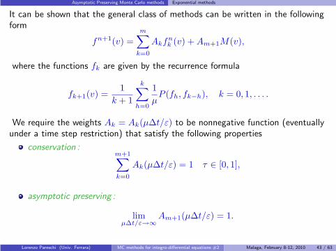
It can be shown that the general class of methods can be written in the followingform
fn+1(v) =
m∑
k=0
Akfnk (v) + Am+1M(v),
where the functions fk are given by the recurrence formula
fk+1(v) =1
k + 1
k∑
h=0
1
µP (fh, fk−h), k = 0, 1, . . . .
We require the weights Ak = Ak(µ∆t/ε) to be nonnegative function (eventuallyunder a time step restriction) that satisfy the following properties
conservation :m+1∑
k=0
Ak(µ∆t/ε) = 1 τ ∈ [0, 1],
asymptotic preserving :
limµ∆t/ε→∞
Am+1(µ∆t/ε) = 1.
Lorenzo Pareschi (Univ. Ferrara) MC methods for integro-differential equations #2 Malaga, February 8-12, 2010 43 / 63

Asymptotic Preserving Monte Carlo methods Exponential methods
RemarksNote that the AP property is not satisfied by the standard first order ETDwhereas it is satisfied by the first order IF scheme. This remains true also forhigher order methods. A modification of ETD methods that satisfy APproperty can be derived using the so called time relaxed methods11
corresponding to
Ak = e−µ∆t/ε(1 − e−µ∆t/ε)k, Am+1 = (1 − e−µ∆t/ε)m+1.
An important property of the coefficients fk(v) appearing in the expansion isthat they are nonnegative and that
∫
IR3
fk(v)φ(v) dv =
∫
IR3
f0(v)φ(v) dv, φ(v) = 1, v, |v|2, ∀ k.
The schemes have a nice probabilistic interpretation. In fact, if fn is aprobability density function so are fn
k for all k and then the schemes describethe next time level fn+1 as a convex combination of probability densityfunctions which makes them suitable for Monte Carlo simulations.
11E.Gabetta, L.P., G.Toscani, ’97. L.P., G.Russo, ’01Lorenzo Pareschi (Univ. Ferrara) MC methods for integro-differential equations #2 Malaga, February 8-12, 2010 44 / 63

Asymptotic Preserving Monte Carlo methods Monte Carlo methods
Asymptotic Preserving Monte Carlo (APMC) Methods
First order scheme (APMC1):Form m = 1 the generalized AP schemes give
fn+1 = A0fn + A1f1 + A2M
The probabilistic interpretation of the above equation is the following.A particle extracted from fn
does not collide with probability A0, (i.e. it is sampled from fn)
collides with another particle extracted from fn with probability A1 (i.e. it issampled from the function f1)
is replaced by a particle sampled from a Maxwellian with probability A2.
Remarks: In this formulation the probabilistic interpretation holds uniformly inµ∆t, at variance with NB, which requires µ∆t < 1. Furthermore, as µ∆t → ∞,the distribution at time n + 1 is sampled from a Maxwellian.In a space non homogeneous case, this would be equivalent to a particle methodfor Euler equations.
Lorenzo Pareschi (Univ. Ferrara) MC methods for integro-differential equations #2 Malaga, February 8-12, 2010 46 / 63

Asymptotic Preserving Monte Carlo methods Monte Carlo methods
Second order APMC scheme
Form m = 2 the generalized AP schemes give
fn+1 = A0fn + A1f1 + A2f2 + A3M,
with f1 = P (fn, fn)/µ, f2 = P (fn, f1)/µ.The probabilistic interpretation of the scheme is the following. Given N particlesdistributed according to fn:
NA0 particles do not collide,
NA1 are sampled from f1, as in the first order scheme,
NA2 are sampled from f2, i.e. NA2/2 particles sampled from fn willundergo dummy collisions with NA2/2 particles sampled from f1,
NA3 particles are sampled from a Maxwellian.
Remarks: Previous MC schemes can be made exactly conservative. This goal isachieved by using a suitable algorithm for sampling a set of particles withprescribed momentum and energy from a Maxwellian.Higher order APMC methods can be constructed similarly.
Lorenzo Pareschi (Univ. Ferrara) MC methods for integro-differential equations #2 Malaga, February 8-12, 2010 47 / 63

Asymptotic Preserving Monte Carlo methods Numerical results
Numerical resultsSpace homogeneous case
Comparison between: NB and APMC1 with the IF coefficients.Test problem: Asymmetric bimodal distribution in 2D.Number of particles: N = 5 × 10⁵
1D Shock wave profiles
Comparison between: NB, APMC1, APMC2, APMC3 with the time relaxedcoefficients.Initial data f(x, v, t) = M(ρ, u, T ), with
ρ = 1.0, T = 1.0, Ma = 3.0, x > 0,
where Ma is the Mach number. The mean velocity is
ux = −Ma√
(γT ), uy = 0,
with γ = 5/3. The values for ρ, u and T for x < 0 are given by theRankine-Hugoniot conditions.Test problem : Hard sphere gas with 50− 100 space cells and 500 particles ineach cell on x > 0.For stationary shocks the accuracy of the methods can be increased bycomputing averages on the solution for t ≫.
Lorenzo Pareschi (Univ. Ferrara) MC methods for integro-differential equations #2 Malaga, February 8-12, 2010 49 / 63

Asymptotic Preserving Monte Carlo methods Numerical results
Homogeneous case
Maxwellian case: L2 norm of the error vs time for the 4-th order moment.DSMC (left) and first order APMC (right) with different time steps.
0 0.1 0.2 0.3 0.4 0.5 0.6 0.7 0.80
1
2
3
4
5
6x 10
−3 Fourth Moment Relaxation. Nanbu scheme
time
L 2 Err
or
DSMC µdt/ε=1DSMC µdt/ε=0.5DSMC µdt/ε=0.25
0 0.1 0.2 0.3 0.4 0.5 0.6 0.7 0.80
1
2
3
4
5
6x 10
−3
time
L 2 Err
or
Fourth Moment Relaxation. Integrating Factor scheme
IFEM µdt/ε=2IFEM µdt/ε=1IFEM µdt/ε=0.5IFEM µdt/ε=0.25
Lorenzo Pareschi (Univ. Ferrara) MC methods for integro-differential equations #2 Malaga, February 8-12, 2010 50 / 63

Asymptotic Preserving Monte Carlo methods Numerical results
Shock profile rarefied regime
1D shock profile: DSMC(+) and first order APMC (×) (top), second order (∗)and third order () APMC (bottom) for ǫ = 1.0 and ∆t = 0.025. From left toright: ρ, u, T . The line is the reference solution.
−4 −3 −2 −1 0 1 2 3 40.8
1
1.2
1.4
1.6
1.8
2
2.2
2.4
2.6
x
ρ(x,
t)
−4 −3 −2 −1 0 1 2 3 4−4.5
−4
−3.5
−3
−2.5
−2
−1.5
x
u x(x,t)
−4 −3 −2 −1 0 1 2 3 40
0.5
1
1.5
2
2.5
3
3.5
4
4.5
5
x
T(x
,t)
−4 −3 −2 −1 0 1 2 3 40.8
1
1.2
1.4
1.6
1.8
2
2.2
2.4
2.6
x
ρ(x,
t)
−4 −3 −2 −1 0 1 2 3 4−4.5
−4
−3.5
−3
−2.5
−2
−1.5
x
u x(x,t)
−4 −3 −2 −1 0 1 2 3 40
0.5
1
1.5
2
2.5
3
3.5
4
4.5
5
x
T(x
,t)
Lorenzo Pareschi (Univ. Ferrara) MC methods for integro-differential equations #2 Malaga, February 8-12, 2010 51 / 63

Asymptotic Preserving Monte Carlo methods Numerical results
Shock profile intermediate regime1D shock profile: DSMC(+) and first order APMC (×) (top), second order (∗)and third order () APMC (bottom) for ǫ = 0.1 and ∆t = 0.0025 for DSMC,∆t = 0.025 for APMC. From left to right: ρ, u, T . The line is the referencesolution.
−4 −3 −2 −1 0 1 2 3 40.8
1
1.2
1.4
1.6
1.8
2
2.2
2.4
2.6
x
ρ(x,
t)
−4 −3 −2 −1 0 1 2 3 4−4.5
−4
−3.5
−3
−2.5
−2
−1.5
x
u x(x,t)
−4 −3 −2 −1 0 1 2 3 40
0.5
1
1.5
2
2.5
3
3.5
4
4.5
5
x
T(x
,t)
−4 −3 −2 −1 0 1 2 3 40.8
1
1.2
1.4
1.6
1.8
2
2.2
2.4
2.6
x
ρ(x,
t)
−4 −3 −2 −1 0 1 2 3 4−4.5
−4
−3.5
−3
−2.5
−2
−1.5
x
u x(x,t)
−4 −3 −2 −1 0 1 2 3 40
0.5
1
1.5
2
2.5
3
3.5
4
4.5
5
x
T(x
,t)
Lorenzo Pareschi (Univ. Ferrara) MC methods for integro-differential equations #2 Malaga, February 8-12, 2010 52 / 63

Asymptotic Preserving Monte Carlo methods Numerical results
Shock profile fluid regime1D shock profile: First order APMC (×) for ǫ = 10−6 and ∆t = 0.025. Fromleft to right: ρ, u, T .
−4 −3 −2 −1 0 1 2 3 40.8
1
1.2
1.4
1.6
1.8
2
2.2
2.4
2.6
x
ρ(x,
t)
−4 −3 −2 −1 0 1 2 3 4−4.5
−4
−3.5
−3
−2.5
−2
−1.5
x
u x(x,t)
−4 −3 −2 −1 0 1 2 3 40
0.5
1
1.5
2
2.5
3
3.5
4
4.5
5
x
T(x
,t)
Lorenzo Pareschi (Univ. Ferrara) MC methods for integro-differential equations #2 Malaga, February 8-12, 2010 53 / 63
Asymptotic Preserving Monte Carlo methods Numerical results
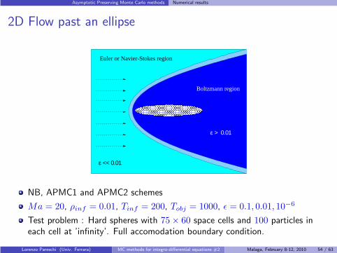
2D Flow past an ellipse
Euler or Navier-Stokes region
Boltzmann region
ε << 0.01
ε > 0.01
NB, APMC1 and APMC2 schemes
Ma = 20, ρinf = 0.01, Tinf = 200, Tobj = 1000, ǫ = 0.1, 0.01, 10−6
Test problem : Hard spheres with 75 × 60 space cells and 100 particles ineach cell at ’infinity’. Full accomodation boundary condition.
Lorenzo Pareschi (Univ. Ferrara) MC methods for integro-differential equations #2 Malaga, February 8-12, 2010 54 / 63
Asymptotic Preserving Monte Carlo methods Numerical results
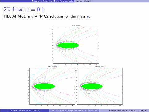
2D flow: ε = 0.1
NB, APMC1 and APMC2 solution for the mass ρ.
2 4 6 8 10 12 14
1
2
3
4
5
6
7
8
9
10
11
DSMC Method
2 4 6 8 10 12 14
1
2
3
4
5
6
7
8
9
10
11
TRMC I Method
2 4 6 8 10 12 14
1
2
3
4
5
6
7
8
9
10
11
TRMC II Method
Lorenzo Pareschi (Univ. Ferrara) MC methods for integro-differential equations #2 Malaga, February 8-12, 2010 55 / 63

Asymptotic Preserving Monte Carlo methods Numerical results
2D flow: ε = 0.1
Transversal and longitudinal sections for the mass ρ at y = 6 and x = 5respectively for ǫ = 0.1 and M = 20; DSMC-NB (), APMC I (+), APMC II (×).
0 2 4 6 8 10 120
0.005
0.01
0.015
0.02
0.025
0.03
0.035
0.04
0.045
0 5 10 150
0.01
0.02
0.03
0.04
0.05
0.06
0.07
0.08
Lorenzo Pareschi (Univ. Ferrara) MC methods for integro-differential equations #2 Malaga, February 8-12, 2010 56 / 63

Asymptotic Preserving Monte Carlo methods Numerical results
2D flow: ε = 0.01
NB, APMC1 and APMC2 solution for the mass ρ.
2 4 6 8 10 12 14
1
2
3
4
5
6
7
8
9
10
11
DSMC Method
2 4 6 8 10 12 14
1
2
3
4
5
6
7
8
9
10
11
TRMC I Method
2 4 6 8 10 12 14
1
2
3
4
5
6
7
8
9
10
11
TRMC II Method
Lorenzo Pareschi (Univ. Ferrara) MC methods for integro-differential equations #2 Malaga, February 8-12, 2010 57 / 63

Asymptotic Preserving Monte Carlo methods Numerical results
2D flow: ε = 0.01
Transversal and longitudinal sections for the mass ρ at y = 6 and x = 5respectively for ǫ = 0.1 and M = 20; DSMC-NB (), APMC I (+), APMC II (×).
0 2 4 6 8 10 120
0.005
0.01
0.015
0.02
0.025
0.03
0.035
0.04
0 5 10 150
0.01
0.02
0.03
0.04
0.05
0.06
Lorenzo Pareschi (Univ. Ferrara) MC methods for integro-differential equations #2 Malaga, February 8-12, 2010 58 / 63

Asymptotic Preserving Monte Carlo methods Numerical results
2D flow: ε = 10−6
NB, APMC1 and APMC2 solution for the mass ρ.
2 4 6 8 10 12 14
1
2
3
4
5
6
7
8
9
10
11
TRMC I Method
2 4 6 8 10 12 14
1
2
3
4
5
6
7
8
9
10
11
TRMC II Method
Lorenzo Pareschi (Univ. Ferrara) MC methods for integro-differential equations #2 Malaga, February 8-12, 2010 59 / 63
Asymptotic Preserving Monte Carlo methods Numerical results
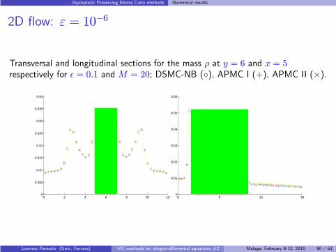
2D flow: ε = 10−6
Transversal and longitudinal sections for the mass ρ at y = 6 and x = 5respectively for ǫ = 0.1 and M = 20; DSMC-NB (), APMC I (+), APMC II (×).
0 2 4 6 8 10 120
0.005
0.01
0.015
0.02
0.025
0.03
0.035
0.04
0 5 10 150
0.01
0.02
0.03
0.04
0.05
0.06
Lorenzo Pareschi (Univ. Ferrara) MC methods for integro-differential equations #2 Malaga, February 8-12, 2010 60 / 63

Asymptotic Preserving Monte Carlo methods Numerical results
2D flow: Number of ”Collisions”
From left to right ǫ = 0.1, 0.01, 0.001; NB (), APMC1 (+), APMC2 (×).
0 50 100 150 200 250 300 350 4000
500
1000
1500
2000
2500
3000
3500
4000
4500
5000
0 50 100 150 200 250 300 350 4000
0.5
1
1.5
2
2.5
3
3.5
x 104
0 50 100 150 200 250 300 350 400 4500
0.5
1
1.5
2
2.5
3
3.5
4x 10
5
Lorenzo Pareschi (Univ. Ferrara) MC methods for integro-differential equations #2 Malaga, February 8-12, 2010 61 / 63

Asymptotic Preserving Monte Carlo methods Further developments
Further developments
There are many different possible improvements of DSMC methods.Typically these methods tackle particular situations like the case of low Machnumber flows12 and simulation of rare events (Stochastic Weighted Particlemethods). 13
Hybrid Monte Carlo methods: Couplings of microscopic stochastic models tomacroscopic deterministic models is highly desirable in many applications.Similar arguments apply also to numerical methods14. Main advantages arereduced variance and improved efficiency close to fluid regimes.
Hydro-guided Monte Carlo: The basic idea consists in obtaining reducedvariance Monte Carlo methods forcing particles to match prescribed sets ofmoments given by the solution of deterministic macroscopic fluid equations15.A similar idea has been used in Information Preserving Monte Carlo. 16
12N. Hadjiconstantinou, T. Homolle, ’0713S.Rjasanow, W.Wagner, ’0514W.E, B.Engquist ’03, L.P. ’05, L.P., G.Dimarco ’06, ’0815P.Degond, G.Dimarco, L.P., ’0916Q.Sun, D.Boyd, ’02.
Lorenzo Pareschi (Univ. Ferrara) MC methods for integro-differential equations #2 Malaga, February 8-12, 2010 63 / 63
Recommended


