Melbourne Institute Working Paper Series
Working Paper No. 14/16Revisiting Okun’s Relationship
Robert Dixon, G. C. Lim and Jan C. van Ours

Revisiting Okun’s Relationship*
Robert Dixon†, G. C. Lim‡ and Jan C. van Ours§ † Department of Economics, The University of Melbourne
‡ Melbourne Institute of Applied Economic and Social Research, The University of Melbourne
§ Department of Economics and CentER, Tilburg University; Department of Economics, The University of Melbourne; Centre for Economic Policy Research;
CESifo; and Institute for the Study of Labor (IZA)
Melbourne Institute Working Paper No. 14/16
ISSN 1328-4991 (Print)
ISSN 1447-5863 (Online)
ISBN 978-0-73-405208-7
March 2016 * The authors thank seminar participants at Marche Polytechnic University (Ancona) and ILO (Geneva), in particular Mattieu Charpe and Niall O’Higgins, and the editor and two anonymous referees for their comments on a previous version of the paper. For correspondence, email <[email protected]>.
Melbourne Institute of Applied Economic and Social Research
The University of Melbourne
Victoria 3010 Australia
Telephone (03) 8344 2100
Fax (03) 8344 2111
Email [email protected]
WWW Address http://www.melbourneinstitute.com

2
Abstract
Our paper revisits Okun’s relationship between observed unemployment rates and output
gaps. We include in the relationship the effect of labour market institutions as well as age and
gender effects. Our empirical analysis is based on 20 OECD countries over the period 1985–
2013. We find that the share of temporary workers (which includes a high and rising share of
young workers) played a crucial role in explaining changes in the Okun coefficient (the
impact of the output gap on the unemployment rate) over time. The Okun coefficient is not
only different for young, prime-age and older workers, it decreases with age. From a policy
perspective, it follows that an increase in economic growth will not only have the desired
outcome of reducing the overall unemployment rate, it will also have the distributional effect
of lowering youth unemployment.
JEL classification: J64
Keywords: Okun’s law, unemployment, equilibrium unemployment rates
1 Introduction
Fluctuations in unemployment and growth go hand in hand and there are numerous
empirical studies of the relationship between the two. The simplest and most widely
cited relationship is “Okun’s law”, i.e. the relationship between unemployment and
the cyclical component of GDP. It is a reduced-form relationship that has underpinned
numerous academic and policy discussions about growth and employment.1
Recent papers suggest that the nature of the relationship has changed over time and
that it is also different during expansions and during recessions. For example, Owyang
and Sekhposyan (2012) using quarterly data over the period 1949-2011 estimated various
specifications of the Okun relationship and found that during the three most recent U.S.
recessions and the Great Recession the unemployment rate was more sensitive to output
growth and output gap fluctuations. Cazes et al. (2013) analysed country-specific changes
in unemployment in the Great Recession and found that Okun’s relationship varied across
countries and time. In some countries unemployment was more responsive and in other
countries it was less responsive to the negative economic growth shock.
Okun (1962) examined three models including a ‘difference version’ which relates
the change in the unemployment rate to the GDP growth rate and a ‘gap version’ which
relates the unemployment rate to the output gap. There is by now an extensive literature
covering both versions. We will be adopting the ‘gap version’ in keeping with our intention
of examining the impact on unemployment of deviations from potential output.2 Also
we will incorporate into Okun’s relationship labour market institutions meaning by that
“the system of laws, norms, or conventions resulting from a collective choice and providing
constraints or incentives that alter individual choices over labour and pay” (Boeri and
van Ours (2013), p 8).
We revisit Okun’s relationship using data from 20 OECD countries over the period
1985-2013. The aim of our paper is to study Okun’s relationship for a range of countries
covering a sample period that includes the Great Recession. In this regard, we will
test for asymmetries in the relationship between the output gap and the unemployment
rate, specifically, whether the Okun coefficient is different in boom and bust periods.
Furthermore, we will examine whether and by how much the Okun coefficient has changed
over time, especially post the Great Recession.
We offer three contributions to the literature. First, we investigate how the relation-
1Okun specified an empirical relationship without clear indications of causality. Perman and Stephan(2015) present a meta-analysis of 269 estimates of Okun’s relationship from 28 studies. According totheir overview about 60 percent of all estimates have real output as the left-hand-side variable, about 75percent use country level data and slightly more than half of the studies use a static model.
2The regression equation in Okun (1962) is u = a+ b(gap). One of the criteria Okun used for judgingthe validity of his estimates is that the results should agree “with the principle that potential GNPshould equal actual GNP when u = 4”, this is because he believed the target rate of unemployment (orfull employment rate of unemployment) was 4%.
3

ship between the (equilibrium) unemployment rate, the output gap and labour market
institutions differ depending upon age and gender. This is an important extension as the
determinants of the equilibrium unemployment rate and the size of the Okun coefficient
are likely to vary across age groups and across gender. Second, we allow labour market
institutions to influence both the equilibrium rate of unemployment and the effect of the
change in the output gap on the unemployment gap (i.e. the Okun coefficient). Third,
we provide estimates of time-varying country-specific equilibrium unemployment rates
and explore differences in the apparent trends in the equilibrium unemployment rates
between countries (especially those in the Eurozone).
The analysis at the age-gender level, taken in conjunction with findings about labour-
institutional factors, allows us to draw some policy implications. We show that equilib-
rium unemployment rates are positively related to union density, the UI replacement rate
and the tax wedge and negatively related to the level of wage coordination and the terms
of trade. We also find that the effects of changes in the output gap on the unemployment
rate decreases with age. From this we infer that an increase in economic growth will
not only reduce the overall unemployment rate but it will also bring about a more than
proportional decline in the youth unemployment rate.
Our paper is structured as follows. In section 2 we provide a short overview of pre-
vious studies and a description of our empirical model. We also present the parameter
estimates of Okun’s relationship assuming to begin with that each country has a con-
stant equilibrium unemployment rate. In section 3 we extend our analysis by allowing
labour market institutional factors to affect the equilibrium unemployment rate while the
effect of the output gap on the unemployment rate is allowed to depend on the share of
temporary workers in employment. Section 4 presents estimates of Okun’s relationship
disaggregated by age and gender. Section 5 concludes.
2 Okun’s relationship at the country-level
2.1 Previous studies
Nickell and Layard (1999), Bertola (1999), Nickell (1997), Siebert (1997) and Arpaia and
Mourre (2005) provide empirical evidence on the impact of labour market institutions on
labour market performance and especially the connection between labour market institu-
tions and the equilibrium or natural rate of unemployment. Important studies that relate
unemployment to labour market institutions but not to the output gap are Blanchard
and Wolfers (2000), Belot and van Ours (2001), Belot and van Ours (2004), and Nickell
et al. (2005). Holmlund (2014) provides a recent discussion on the relevance of various
labour market institutions. van Ours (2015) estimates a ‘difference version’ of Okun’s
4

relationship linking changes in unemployment to labour market institutions.
Previous studies relating the unemployment gap (or the unemployment rate) to the
output gap and to labour market institutions mostly look at a sub-set of OECD countries.
All of the studies we have examined find that the unemployment rate is negatively related
to the output gap. The findings on the relationship between unemployment rates and
labour market institutions vary. It is common for studies to include the unemployment
benefit replacement rate and sometimes measures of the duration and eligibility require-
ments.3 All of the studies we have looked at find a positive relationship between the
unemployment rate and the replacement rate. Most studies also include union density as
an explanatory variable. While Adams and Coe (1990), Coe (1990) and Scarpetta (1996)
find a positive relationship between the unemployment rate and union density, Elmeskov
et al. (1998) and Bassanini and Duval (2009) do not find any statistically significant
relationship between the two.
Many researchers include a measure of employment protection as an explanatory vari-
able. Again there are mixed results. While Scarpetta (1996) and Elmeskov et al. (1998)
find a positive relationship between the unemployment rate and employment protection
Griffith et al. (2007), Bassanini and Duval (2009) and Vandenberg (2010) do not find any
statistically significant relationship between them.
The influence of wage coordination and/or centralisation on the unemployment rate
has also been examined. While Vandenberg (2010) finds no evidence of any impact of
centralisation, others (eg Scarpetta (1996) and Elmeskov et al. (1998)) conclude that
there is a ‘hump-shaped’ relationship between the unemployment rate and centralisation
as suggested by Calmfors and Driffill (1988).
The most common additional explanatory variables included in studies are active
labour market programs (Scarpetta (1996) and Elmeskov et al. (1998)), the tax wedge
and non-wage labour costs (Adams et al. (1987), Coe (1990), Scarpetta (1996), Elmeskov
et al. (1998), Griffith et al. (2007) and Bassanini and Duval (2009)), the real exchange rate
(Adams et al. (1987) and Griffith et al. (2007)) and the terms of trade (Scarpetta (1996)).
Other (less common) variables included are the minimum wage (Adams and Coe (1990),
Coe (1990) and Elmeskov et al. (1998)), the rate of structural change (Herwartz and
Niebuhr (2011)), the level of product market regulation (Bassanini and Duval (2009))
and demographic factors such as the proportion of the labour force who are ‘young’
(Adams et al. (1987), Adams and Coe (1990)).
The studies noted cover different sample periods. Ball et al. (2013) studied Okun’s
relationship for the US from 1948 to 2011 and for 20 OECD countries from 1980 to 2011.
They concluded that there was a strong and stable relationship “by the standards of
3Bassanini and Duval (2009) and Vandenberg (2010) for example include measures of the durationand eligibility requirements.
5

macroeconomics” in most countries although the magnitude of the relationship between
output and unemployment varied across countries. Pereira (2013) analysed quarterly US
data from 1948:1 to 2012:4 and found that there are asymmetries in Okun’s relationship
with a weaker relationship between economic growth and unemployment during periods
of expansion.
2.2 Empirical Model
Okun’s law is an empirical relationship between output and unemployment which in its
‘gap’ version may be written as
(u− u∗) = −Φ(y − y∗) (1)
where u is the unemployment rate; y is (log) output; y∗ is (log) potential output, u∗
indicates the equilibrium unemployment rate and Φ is the Okun coefficient.
Our baseline econometric model, for a panel dataset across countries and time periods
is:
uit = αi − Φ(yit − y∗it) + εit (2)
E(εitεjt) = σij
E(εisεit) = 0; s 6= t
The subscript i denotes the country and t is time in years. αi are the country-specific
fixed effects (which, in this model are equal to u∗i the country-specific equilibrium unem-
ployment rates). It is assumed that the errors are related cross-sectionally (i.e. across
countries), but not across periods (i.e. years). The model is estimated by GLS allowing
for cross-sectional heteroskedasticity.
As is common in the literature, the output gap is estimated using the Hodrick-Prescott
filter. Specifically, the HP filter is a two-sided linear filter that computes the smoothed-
series y∗ of y by minimising the variance of y around y∗ subject to a penalty function
that constrains the change in the trend growth of y∗:
Θ =T∑t=1
(yt − y∗t )2 + λ
T−1∑t=2
((y∗t+1 − y∗t )− (y∗t − y∗t−1))2 (3)
The penalty parameter λ controls the smoothness of the series and the suggested value
by HP is 100.4
4Ravn and Uhlig (2002) suggest 6.25 for annual data. The results using this value of λ are essentiallythe same as those reported using λ = 100. As an alternative to the HP filter we used a Band-pass filterand a Beveridge-Nelson decomposition but neither led to any change in our main findings.
6

2.3 Data
Because of data availability the focus of the analysis is on 20 OECD countries over the
period 1985-2013. There are 5 countries outside Europe (Australia, Canada, Japan, New
Zealand and the United states) and 15 countries in Europe of which 10 adopted the Euro
(Austria, Belgium, Finland, France, Germany, Ireland, Italy, Netherlands, Portugal and
Spain) and 5 did not (Denmark, Norway, Sweden, Switzerland and the United Kingdom).
Output gaps are created for each country in the data set. By construction the mean
value of each country’s output gap is zero. Figure 1 provides information about the
evolution over time of the unemployment rates and the (inverse of the) output gap for
the 20 countries in our sample. The vertical scales show the difference in the fluctuations
in unemployment rate and/or output gap across the panel. Clearly, in all countries
variations in unemployment rates and output gaps go hand in hand. The output gap
associated with the Great Recession, which (because of the inverse scale is presented as a
strong increase) has had a greater impact on some countries than on others. In Australia
for example the increase in unemployment is relatively small while for Ireland, Portugal,
Spain and the US for example, the increase was relatively large. While unemployment in
Germany and the United States fell after the Great Recession, in other countries such as
France, Italy, Portugal and Spain unemployment continued to be high.
– Figure 1 and Table 1 about here –
2.4 Parameter estimates
Table 1 shows the parameter estimates of the baseline version of Okun’s relationship
i.e., the estimation of equation (2) above which assumes that the equilibrium rate of
unemployment (u*) varies across countries but, for each country, it is constant over time.
The GDP-gap has a significant and negative effect on the unemployment rate. This is
not surprising given the high correlation between the two as shown in Figure 1.
Table 1 also shows that there is considerable cross-country variation in the implied
equilibrium unemployment rates, with estimates of α ranging from a low 3% in Switzer-
land to a high 17% for Spain. There is strong cross-country correlation between the
average unemployment rate and the estimated values of the equilibrium unemployment
rate.
– Table 2 about here –
Table 2 shows the parameter estimates when we modify equation (2) to allow for
asymmetry, in the sense that positive/negative output gaps have different effects on
unemployment. As shown in the second column of Table 2 we are unable to reject the
hypothesis of symmetry. The third column shows parameter estimates if we allow the
effect of the output gap on unemployment to be different after the Great Recession from
7

that before the Great Recession. We cannot reject the hypothesis that they are different
for this simple model.
3 Introducing labour market institutions
3.1 Labour market institutions
So far, equilibrium unemployment rates have been assumed to be constant over time.
However, previous studies suggest that labour market institutions may affect the equilib-
rium unemployment rate. We investigate the significance of the following labour market
institutions: union coverage, union density, wage coordination, UI replacement rate, em-
ployment protection legislation and the tax wedge and additionally the terms of trade.
Furthermore, since labour markets have become more flexible in the past decades we
investigate whether the responsiveness of unemployment to a change in the output gap
is influenced by the ratio of temporary workers to total employees since the larger the
share of temporary workers the easier (ceteris paribus) the adjustment of employment
to output shocks and thus (ceteris paribus) the bigger the effect of an output shock on
unemployment.
– Figure 2 about here –
Figure 2 gives a graphical representation of the developments in the labour market
institutions. Appendix A provides details on the data used. Each of the graphs in
Figure 2 plots, for each country, the values of the variables at two points in time - 1985
and 2013. Clearly, for many countries not much has happened between these two years
as they are on the diagonal or close to it. However, there are also some exceptions.
The graphs in panel a indicate the evolution in union coverage (left) and union density
(right). Union coverage is high in Austria, Belgium and France and low in Japan and the
United States. If a country is below the diagonal it indicates a drop in union coverage or
union density. The fall in union coverage has been greatest in Australia, New Zealand,
Portugal and the United Kingdom. For these countries, the fall in union density has been
substantial as well. Union density is high in the Scandinavian countries (which has to do
with unemployment insurance (UI) benefits run by unions) while union density is low in
France, the United States and Spain. Panel b shows the evolution of wage coordination
(left) and UI replacement rate (right). There is quite a wide range of wage coordination
with Canada, the United Kingdom and the United States having the lowest value of
the indicator. In Australia and New Zealand wage coordination has fallen while in Italy
wage coordination has substantially increased. With respect to the UI replacement rate
in most countries there was a decrease over our sample period but for Italy, Portugal
and Norway there was a substantial increase. Panel c shows the developments in the tax
8
wedge (left) and Employment Protection Legislation (right). In many countries the tax
wedge did not change a lot but in Ireland there was a substantial drop while in Japan
there was a substantial increase. Finally, as shown in the bottom-right graph, in many
countries EPL shows persistence over time but there are also countries for which EPL
was reduced a lot (Belgium, Italy, Germany, Portugal, Spain and Sweden).
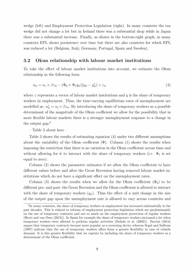
3.2 Okun relationship with labour market institutions
To take the effect of labour market institutions into account, we estimate the Okun
relationship in the following form:
uit = αi + βzit − (Φ0 + Φ1qit)(yit − y∗it) + εit (4)
where z represents a vector of labour market institutions and q is the share of temporary
workers in employment. Thus, the time-varying equilibrium rates of unemployment are
modelled as: u∗it = αi +βzit. By introducing the share of temporary workers as a possible
determinant of the magnitude of the Okun coefficient we allow for the possibility that in
more flexible labour markets there is a stronger unemployment response to a change in
the output gap.5
– Table 3 about here –
Table 3 shows the results of estimating equation (4) under two different assumptions
about the variability of the Okun coefficient (Φ). Column (1) shows the results when
imposing the restriction that there is no variation in the Okun coefficient across time and
without allowing for it to interact with the share of temporary workers (i.e. Φ1 is set
equal to zero).
Column (2) shows the parameter estimates if we allow the Okun coefficient to have
different values before and after the Great Recession having removed labour market in-
stitutions which do not have a significant effect on the unemployment rates.
Column (3) shows the results when we allow for the Okun coefficient (Φ0) to be
different pre- and post- the Great Recession and the Okun coefficient is allowed to interact
with the share of temporary workers (qit). Thus the effect of a unit change in the size
of the output gap upon the unemployment rate is allowed to vary across countries and
5In many countries, the share of temporary workers in employment has increased substantially in thepast decades. This is related to reforms of employment protection legislation which are predominantlyon the use of temporary contracts and not so much on the employment protection of regular workers(Boeri and van Ours (2013)). In Spain for example the share of temporary workers increased a lot whentemporary workers were allowed to perform regular activities (Dolado et al. (2002)). Faccini (2014)argues that temporary contracts became more popular as a screening device whereas Segal and Sullivan(1997) indicate that the use of temporary workers offers firms a greater flexibility in case of volatiledemand. It is this greater flexibility that we capture by including the share of temporary workers as adeterminant of the Okun coefficient.
9

across time (as the share of temporary workers varies across countries and across time).6
Column (4) of Table 3 shows the results of equation (4) on the assumption that the Okun
coefficient (Φ0) is the same pre and post the Great Recession (consistent with the findings
reported in column 3).
Inspection of the estimated values of the coefficients and their p-values in the top part
of the table (the part which reports coefficients on the output gaps) and also the result
of a Wald test for a significant difference between the value of the Okun coefficient before
and after the Great Recession (this is reported at the bottom of the Table) leads us to
conclude that: (a) For the base model we reject the hypothesis that the Okun coefficient
has remained the same over time. (b) Once we introduce labour market institutions
and allow the size of the Okun coefficient to vary with the share of temporary workers
the magnitude of the Okun coefficient pre and post the Great Recession are virtually
identical. This suggests that the apparent change in the Okun coefficient after the Great
Recession noted earlier when discussing Table 2 may be due to the omission of labour
market institutions. (c) The sign of the coefficient on the interaction term implies that
the larger is the share of temporary workers the ‘larger’ (i.e. the more negative) is the
impact of a change in the output gap on the unemployment gap. Since the share of
temporary workers has been rising on average and across all age groups, this implies that
Okun’s coefficient i.e. the impact of a change in the output gap on the unemployment
gap has likely been trending upwards (becoming more negative) over time. Note that
similar conclusions were reached in an IMF study of Okun’s Law. “The responsiveness
of unemployment to output has increased over the past 20 years in many countries. This
reflects (inter alia) the greater use of temporary employment contracts.” (International
Monetary Fund (2010), Ch 3, p 1).
We turn now to the effect of labour market variables in explaining differences in the
unemployment rate across countries and over time. The signs and significance of most
these variables are robust across the different specifications. The results given in column
(1) in the lower part of Table 3 show that there is no significant relationship between the
(equilibrium) unemployment rate and union coverage (defined as the proportion of work-
ers covered by collective bargaining) but we find a significant and, as expected, positive
relationship between the unemployment rate and union density (defined as the proportion
of workers who are union members). Furthermore, wage coordination has a significant
negative effect on unemployment while the UI replacement rate has a significant posi-
tive effect. Employment protection legislation has no significant effect on unemployment.
6We think that compared with non-temporary workers a higher proportion of temporary workers arelikely to move between employment and not in the labour force (or ‘inactive’) relative to the proportionwho move between employment and unemployment. As a result, the effect of a change in the output gap(and thus the number of temporary workers employed) may impact more on the labour force participationrate than on the unemployment rate.
10
The tax wedge has a significant positive effect7 and terms of trade has a significant neg-
ative effect on unemployment. We removed union coverage and employment protection
legislation from the analysis.8
As a check of robustness we also estimated the model for different groups of countries.
Column (5) of Table 3 shows the parameter estimates if we restrict the sample to 15
European countries. Not reported are estimates for the 13 European Union countries and
for the 10 Euro-zone countries. The results are robust across these different combinations
of European countries.
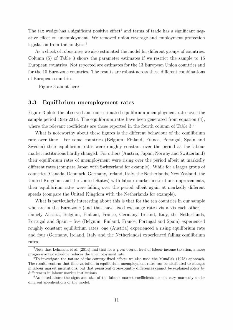
– Figure 3 about here –
3.3 Equilibrium unemployment rates
Figure 3 plots the observed and our estimated equilibrium unemployment rates over the
sample period 1985-2013. The equilibrium rates have been generated from equation (4),
where the relevant coefficients are those reported in the fourth column of Table 3.9
What is noteworthy about these figures is the different behaviour of the equilibrium
rate over time. For some countries (Belgium, Finland, France, Portugal, Spain and
Sweden) their equilibrium rates were roughly constant over the period as the labour
market institutions hardly changed. For others (Austria, Japan, Norway and Switzerland)
their equilibrium rates of unemployment were rising over the period albeit at markedly
different rates (compare Japan with Switzerland for example). While for a larger group of
countries (Canada, Denmark, Germany, Ireland, Italy, the Netherlands, New Zealand, the
United Kingdom and the United States) with labour market institutions improvements,
their equilibrium rates were falling over the period albeit again at markedly different
speeds (compare the United Kingdom with the Netherlands for example).
What is particularly interesting about this is that for the ten countries in our sample
who are in the Euro-zone (and thus have fixed exchange rates vis a vis each other) –
namely Austria, Belgium, Finland, France, Germany, Ireland, Italy, the Netherlands,
Portugal and Spain – five (Belgium, Finland, France, Portugal and Spain) experienced
roughly constant equilibrium rates, one (Austria) experienced a rising equilibrium rate
and four (Germany, Ireland, Italy and the Netherlands) experienced falling equilibrium
rates.
7Note that Lehmann et al. (2014) find that for a given overall level of labour income taxation, a moreprogressive tax schedule reduces the unemployment rate.
8To investigate the nature of the country fixed effects we also used the Mundlak (1978) approach.The results confirm that time variation in equilibrium unemployment rates can be attributed to changesin labour market institutions, but that persistent cross-country differences cannot be explained solely bydifferences in labour market institutions.
9As noted above the signs and size of the labour market coefficients do not vary markedly underdifferent specifications of the model.
11

Given the model of unemployment used to generate the equilibrium rates of unem-
ployment in this paper, the explanation for the different trends in the equilibrium rate
reflect different trends in labour market institutions. We make two observations here
about the equilibrium rates of unemployment. To the extent for example that different
trends in the equilibrium rate reflect different trends at the national levels in the amount
of frictional unemployment - where frictional unemployment in this context is defined
as a situation where the characteristics of an unemployed worker in one EU country are
matched by the characteristics of a vacancy in that or another EU country - then facili-
tating labour mobility would seem to be the desirable and effective policy response. To
the extent that low mobility is a reflection of current labour market institutions a change
in the institutions in a way that would enhance mobility will lead to convergence in the
equilibrium rates. Another example would be differences in the equilibrium rate resulting
from differences in the UI replacement rate, differences which effectively ensures differ-
ences in the minimum reservation wage. Here again a harmonisation of labour market
institutions - and specifically in this case social protection objectives and policies - would
lead to convergence in the equilibrium rates.
3.4 Sensitivity analysis
To explore the robustness of our findings we performed additional sensitivity analyses.
First, we added a common global factor into the Okun model. As discussed in more detail
in Appendix B1, this hardly influences our parameter estimates. Second, we introduced
product market regulation as an additional explanatory variable. Although product mar-
ket regulation has a significant positive effect on unemployment rates it has not been
retained. This is because product market regulation and union density are highly cor-
related and it is not clear what product market regulation is picking up (see for details
Appendix B2). Furthermore, because of the reunification of Germany, we estimated a
model allowing for a shift in the German data at that time. This did not lead to any
essential difference in our results. Finally, because changes in the collection of the Eu-
ropean labour force survey might have introduced breaks in the unemployment series in
2003, data for 2003 was dropped from our sample period as a robustness check. This did
not lead to any change in our main findings.
4 Okun’s relationship by age and gender
4.1 Unemployment rates by age and gender
There are large and persistent differences in the labour market characteristics of workers
according to their age and gender. Table 4 provides an overview of country-specific
12

averages of the unemployment rates by age and gender. Clearly, there are substantial
differences both within and between countries. Youth unemployment rates are on average
twice as high as unemployment rates among prime age workers whereas unemployment
rates among old men and women are on average the lowest. There are differences between
unemployment rates of young men and young women but the dominant difference amongst
the young is according to country, not gender. Whereas on average youth unemployment
rates in Austria, Germany, Japan and Switzerland are below 10 percent, they are above
25 percent for young men and women in Italy and Spain. There are also differences
for prime age workers but they are substantially smaller in absolute terms. The lowest
unemployment rates over the time period for prime age men and women are in Norway
and Japan (below 4 percent). The highest unemployment rates for old men are in Spain
with 10.2 percent and for old women in Germany with almost 11 percent, while the lowest
rates for old men and women are in Norway (both less than 2 percent).
– Table 4 and Figure 4 about here –
Figure 4 shows the evolution of unemployment rates over the period 1985-2013 aver-
aged for the 20 countries and disaggregated by age and gender. The unemployment rates
shown in panel a are very different depending on age. The unemployment rates of young
individuals are by far the highest and they fluctuate much more than the unemployment
rates of prime age and old individuals. Conditional on age the differences between men
and women are small.
4.2 Modified Okun relationship
It is well-known and has been illustrated in the previous subsection that unemployment
rates of young workers are on average higher and more volatile than unemployment rates
of prime age and old workers (Bell and Blanchflower (2011)). There are various reasons
why Okun’s relationship may be age-specific.10 Compared to older workers young workers
have less company-specific skills and less dismissal protection (Dunsch (2015), O’Higgins
(1997)). Furthermore, to the extent that age is related to experience, Becker (1964)
argues that the amount of specific training affects the incentives of firms and workers
to separate - an idea developed by Cairo and Cajner (2014). Since the labour market
position of females is different from the labour market position of males it is likely that
Okun’s relationship is both age and gender-specific.
10There are three studies that have investigated age-specific versions of the difference form of Okun’slaw. Hutengs and Stadtmann (2013) estimated Okun’s relationship over the period 1984-2011 for 11Eurozone countries and five age groups. Zanin (2014) studied 5 age cohorts by gender for 33 OECDcountries over the period 1998-2012. Hutengs and Stadtmann (2014) estimated Okun’s relationship forfive Scandinavian countries and five age groups over the period 1984-2011. All studies found that thechange in unemployment is more sensitive to economic growth for young workers than for prime age andolder workers.
13

We begin by modifying our baseline model (2) to allow estimation of the unemploy-
ment rates by age and gender for 6 groups:
uikt = αik − Φk(yit − y∗it) + εikt (5)
where k represents 3 age groups (15-24, 25-54, 55-64) for both males and females (k =
1,..,6). We assume that the equilibrium rates not only differ across countries, they also
differ across age groups.
4.3 Parameter estimates
The parameter estimates of equation (5) are presented in Table 5. There are clear dif-
ferences in the Okun relationship by age and gender. To start with, the effect of the
GDP-gap on the unemployment rate decreases with age. Whereas the Okun coefficient
has a value of 1.14 for young males, it has a value of 0.56 for prime age males and a
value of 0.45 for old males. A similar pattern though at smaller magnitudes is present
for females. When output changes, the effect on unemployment rates is more than twice
as large for young workers than it is for older workers. This explains Figure 4 which
shows that, while fluctuations in unemployment rates are highly correlated across age
and gender, they are substantially larger for young workers.
– Table 5 and Figure 5 about here –
Figure 5 shows the cross-country relationship between the estimated equilibrium un-
employment rates for young and prime age workers, separately for males and females.
Panel a shows the relationship for males. There is across countries a strong correlation
between the unemployment rates of young and prime age males. The ratio of the two
unemployment rates is about 2.5. Clear outliers are Italy with a relatively high male
youth unemployment rate and Germany with a relative low male youth unemployment
rate. Panel b shows the same relationship for females. In many countries the female
equilibrium unemployment rates are substantially higher for both prime age and young
females. Across countries Italy and Germany are likewise outliers, as for males.
Finally, we allow labour institutions to affect the separate Okun’s relationships by age
and gender (thereby allowing the equilibrium rates and the effect of the output gap on
the unemployment rate to be time-varying); for k = 1,..,6
uikt = (αik + βkzit)− (Φ0 + Φkqikt)(yit − y∗it) + εikt (6)
where z represents labour market institutions, q is the share of temporary workers and
k represents 3 age groups (15-24, 25-54, 55-64) for both males and females. As shown in
panel b of Figure 4 the share of temporary workers is substantially higher among young
14

workers and also increasing much faster than among prime age and older workers. The
increase in the share of temporary workers over the sample period, is on average about
10 percentage-point higher from 25 to 35 percent.
Table 6 shows the relevant parameter estimates of equation 6. Clearly, the estimated
gap-coefficients are not very different from those in Table 5. The share of temporary
workers has a significant effect on the gap-coefficient except for older workers. This may
be due to the low share of old temporary workers as well as with the relative stability
of that share. The parameter estimate for the interaction term between the output gap
and their share of temporary workers is smaller for young workers but one has to take
into account the fact that the share of temporary workers is much higher and increasing.
Finally, the magnitude of the effects of labour market institutions on the unemployment
rates are age and gender specific. In particular, a high level of wage coordination seems to
be mostly beneficial for young workers. A possible explanation is that a high level of wage
coordination more strongly internalizes the unemployment effects of wage negotiations.
Especially youngsters suffer high unemployment rates. Therefore, they may be more
affected by a high level of wage negotiations, i.e. for them the dampening effect on
unemployment rates is strongest. Nevertheless, the overall results are not very different
from those presented in Table 3.
– Table 6 about here –
As a final sensitivity analysis we included in the estimates for old workers, the aver-
age age of retirement. While the variable is significantly different from zero, the other
parameter estimates were hardly affected (see Appendix B3 for details).
5 Conclusions
Okun’s empirical relationship has been shown repeatedly, in a large number of studies
to be an enduring stylised fact. In this paper we revisit Okun’s relationship using a
hybrid specification, namely we relate the unemployment rate, on the one hand, to the
(determinants of the) equilibrium unemployment rate and the output gap, on the other.
The computation of the output gap follows standard practice in the literature, namely
the output gap is the difference between the actual (log) GDP less the trend (log) out-
put (estimated using the Hodrick-Prescott filter). However, we augment the estimating
equation to allow labour market institutional factors to affect the equilibrium rate of
unemployment and moreover we also allow the share of temporary workers to affect the
relationship between the output gap and the unemployment rate. These features im-
proved the analysis firstly, because the introduction of institutional labour factors which
changed over time allowed the derivation of time-varying equilibrium unemployment rates
and secondly, the introduction of a term to capture flexibility in the labour market (the
15

share of temporary workers) was particularly important as it captured effectively changes
in the Okun coefficient over time and allows us to avoid the need to arbitrarily impose dif-
ferent coefficients pre- and post- the Great Recession. Introducing an interaction between
the share of temporary workers and the output gap is also relevant from an economic
point of view. Labour markets have become more flexible in the past decades and es-
pecially among young workers the share of temporary workers is not only high but also
increasing fast. In terms of Okun’s relationship this means that the unemployment effects
of shocks to output have increased over time.
The empirical analysis was conducted using a panel dataset covering 20 OECD coun-
tries over the sample period 1985-2013. Although the observations were diverse over space
and time, they are all indicative of economic behaviour in advanced economies linked by
significant trade and financial flows. The study focused on drawing broad inferences, but
we have also drawn attention to country-specific differences. We find that the equilibrium
unemployment rate is (as expected) positively related to union density, the replacement
rate and the tax wedge and is (again as expected) negatively related to the level of the
wage coordination and the terms of trade.
Finally, since the unemployment rates for younger workers (aged between 15 and 24
years) were considerably higher than unemployment rates of both prime age and older
workers, we also estimated Okun’s relationship using unemployment rates disaggregated
by age and gender. The results provide statistically significant empirical evidence that
the effect of changes in the output gap on the unemployment rate decreases with age. In
particular, that a positive change in the output gap is likely to result in a greater reduction
in unemployment among younger job-seekers compared to the other age groups. From
a policy perspective, it follows that an increase in economic growth (to close the output
gap) will not only have the desired outcome of reducing the unemployment rate, it will
also have the distributional effect of lowering youth unemployment.
16

References
Adams, C. and D. T. Coe (1990). A systems approach to estimating the natural rate of unem-ployment and potential output for the United States. Staff Papers-International MonetaryFund 37 (2), 232–293.
Adams, C., P. Fenton, and F. Larsen (1987). Potential output in major industrial countries.Staff studies for the World Economic Outlook, Washington, IMF.
Arpaia, A. and G. Mourre (2005). Labour market institutions and labour market performance:A survey of the literature. Economic Paper 238, European Commission.
Ball, L., D. Leigh, and P. Loungani (2013). Okun’s law: fit at 50? NBER Working Paper18668.
Bassanini, A. and R. Duval (2006). Employment patterns in OECD countries: reassessing therole of policies and institutions. Economics Department Working Papers 486, OECD.
Bassanini, A. and R. Duval (2009). Unemployment, institutions and reform complementari-ties: Re-assessing the aggregate evidence for OECD countries. Oxford Review of EconomicPolicy 25, 40–59.
Becker, G. S. (1964). Human Capital: A Theoretical and Empirical Analysis with Special Ref-erence to Education. Columbia University Press, New York.
Bell, D. and D. Blanchflower (2011). Young people and the Great Recession. Oxford Review ofEconomic Policy 27, 241–267.
Belot, M. and J. C. van Ours (2001). Unemployment and labor market institutions: an empiricalanalysis. Journal of Japanese and International Economics 15, 1–16.
Belot, M. and J. C. van Ours (2004). Does the recent success of some OECD countries inlowering their unemployment rate lie in the clever design of their labor market reforms?Oxford Economic Papers 56, 621–642.
Bertola, G. (1999). Handbook of labor economics, Chapter Microeconomic perspectives onaggregate labor markets, pp. 2985–3028. Amsterdam: North-Holland.
Blanchard, O. and J. Wolfers (2000). The role of shocks and institutions in the rise of Europeanunemployment: The aggregate evidence. Economic Journal 110, 1–33.
Boeri, T. and J. C. van Ours (2013). The Economics of Imperfect Labor Market, 2nd edition.Princeton University Press.
Cairo, I. and T. Cajner (2014). Human capital and unemployment dynamics: Why moreeducated workers enjoy greater employment stability. Staff Working Paper 2014-09, FederalReserve Board, Washington.
Calmfors, L. and J. Driffill (1988). Bargaining structure, corporatism and macroeconomicperformance. Economic Policy 3 (6), 13–61.
Cazes, S., S. Verick, and F. Al Hussami (2013). Why did unemployment respond so differentlyto the global financial crisis across countries? Insights from Okun’s Law. IZA Journal ofLabor Policy 2, 1–18.
17

Coe, D. (1990). Structural determinants of the natural rate of unemployment in Canada. StaffPapers-International Monetary Fund 37 (1), 94–115.
Dolado, J. J., C. Garcia-Serrano, and J. F. Jimeno (2002). Drawing lessons from the boom oftemporary jobs in Spain. Economic Journal 112, F270–F295.
Dunsch, S. (2015). Okun’s law and youth unemployment in Germany and Poland. DiscussionPaper 373, European University Viadrina Frankfurt.
Elmeskov, J., J. P. Martin, and S. Scarpetta (1998). Key lessons for labor market reforms:Evidence from OECD countries’ experience. Swedish Economic Policy Review 5(2), 205–252.
Faccini, R. (2014). Reassessing labour market reforms: Temporary contracts as a screeningdevice. Economic Journal 124, 167–200.
Griffith, R., R. Harrison, and G. Macartney (2007). Product market reforms, labour marketinstitutions and unemployment. Economic Journal 117, C142–C166.
Herwartz, H. and A. Niebuhr (2011). Growth, unemployment and labour market institutions:evidence from a cross-section of EU regions. Applied Economics 43 (30), 4663–4676.
Holmlund, B. (2014). What do labor market institutions do? Labour Economics 30, 62–69.
Hutengs, O. and G. Stadtmann (2013). Age effects in Okun’s law within the Eurozone. AppliedEconomics Letters 20 (9), 821–825.
Hutengs, O. and G. Stadtmann (2014). Age- and gender-specific unemployment in Scandinaviancountries: An analysis based on Okun’s law. Comparative Economic Studies 56, 567–580.
International Monetary Fund (2010). World Economic Outlook. IMF, Washington.
Lehmann, E., C. Lucifora, S. Moriconi, and B. Van der Linden (2014). Beyond the labourincome tax wedge: the unemployment-reducing effect of tax progressivity. Discussion paperno. 8276, IZA.
Mundlak, Y. (1978). On the pooling of time series and cross-section data. Econometrica 46,69–85.
Nickell, S. (1997). Unemployment and labor market rigidities: Europe versus North America.Journal of Economic Perspectives 11, 55–74.
Nickell, S. J. and R. Layard (1999). Handbook of Labor Economics, Chapter Labor marketinstitutions and economic performance, pp. 3029–3084. Amsterdam: North-Holland.
Nickell, S. J., L. Nunziata, and W. Ochel (2005). Unemployment in the OECD since the 1960s;what do we know? Economic Journal 115, 1–27.
OECD (2013). Employment Outlook. OECD: Paris.
O’Higgins (1997). The challenge of youth unemployment. International Social Security Re-view 50, 63–93.
Okun, A. M. (1962). Potential GNP: Its measurement and significance. Proceedings of Businessand Economics Statistics Section, American Statistical Association, 331-356.
18

Owyang, M. T. and T. Sekhposyan (2012). Okun’s law of the business cycle: Was the GreatRecession all that different? Federal Reserve Bank of St. Louis Review (September/October),399–418.
Pereira, R. M. (2013). Okun’s law across the business cycle and during the Great Recession: aMarkov switching analysis. College of William and Mary Working Paper 139.
Perman, R. and G. Stephan (2015). Okun’s law - a meta analysis. The Manchester School 83 (1),101–126.
Ravn, M. and H. Uhlig (2002). On adjusting the Hodrick-Prescott filter for the frequency ofobservations. Review of Economics and Statistics 84 (2), 371–380.
Scarpetta, S. (1996). Assessing the role of labour market policies and institutional settings onunemployment: A cross-country study. OECD Economic studies 26 (1), 43–98.
Segal, L. M. and D. G. Sullivan (1997). The growth of temporary services work. Journal ofEconomic Perspectives 11, 117–136.
Siebert, H. (1997). Labor market rigidities: at the root of unemployment in Europe. Journalof Economic Perspectives 11, 37–54.
van Ours, J. C. (2015). The Great Recession was not so Great. Labour Economics 34, 1–12.
Vandenberg, P. (2010). Impact of labor market institutions on unemployment: results from aglobal panel. Asian development bank economics working paper series no 219, Asian Devel-opment Bank.
Visser, J. (2011). Data base on institutional characteristics of trade unions, wage setting, stateintervention and social pacts, 1960-2010, version 3.0. Technical report, Amsterdam Institutefor Advance Labor Studies AIAS, University of Amsterdam.
Zanin, L. (2014). On Okun’s law in OECD countries: an analysis by age cohorts. EconomicsLetters 125, 243–248.
19
Appendix A: Details on data
1. Unemployment and employment data: Unemployment national averages for 20 countries.
Sources : (1) 1985-2003: Bassanini and Duval (2006), (2) 2004-2013: OECD labour force
statistics. Unemployment rates and employment rates by gender and age. Source: OECD
labour force statistics.
2. GDP. Source: World Bank.
3. Unions and wage bargaining: Visser (2011) published a data base for the period 1960
to 2010 on institutional characteristics of trade unions, wage setting, state intervention
and social pacts. In case of missing observations in recent years numbers are assumed
to be constant from the last available year onwards. From this database the following
series are used: 1. Union density: union membership as a percentage of wage and salary
earners in employment. 2. Union coverage: employees in workplaces covered by unions
or works councils as a percentage of all wage and salary earners in employment; adjusted
for the possibility that some sectors or occupations are excluded from the right to bar-
gain. 3. Coordination of wage bargaining: discrete values ranging from 5 (economy-wide
bargaining) to 1 (fragmented bargaining, mostly at company level).
4. UI replacement rate: unemployment insurance and unemployment assistance benefits as
a percentage of the Average Production Worker wage; this OECD summary measure
is defined as the average of the gross unemployment benefit replacement rates for two
earnings levels, three family situations and three durations of unemployment. Series 1985
to 2005 available for odd years – even years are calculated as average of adjacent odd years;
from 2006 onwards unemployment insurance and unemployment assistance benefits as a
percentage of the Average Worker wage; the jump in series from 2005 to 2006 has been
accounted for by the authors. Source: OECD statistics.
5. Tax wedge: One-earner married couple at 100% of average earnings with 2 children
expressed as a percentage of labour costs. Source: OECD Taxing Wages - Comparative
tables, Average Tax Wedge (%).
6. Employment protection legislation; scale 0–6, low to high. Series available from 1985.
Source: OECD (2013).
7. Average retirement age: OECD average effective age of retirement calculated as a weighted
average of (net) withdrawals from the labour market at different ages over a 5-year period
for workers initially aged 40 and over. Source: OECD labour force statistics.
8. Terms of trade: Calculated as the ratio of the Deflators for Exports and Imports. Source:
OECD Economic Outlook - Country Tables Annual Data, Deflators and CPI.
9. Share of temporary workers, average and by gender and age. Source: OECD labour force
statistics
20
10. Product market regulation: Summary indicator of regulatory impediments to product
market competition in seven non-manufacturing industries. Source: OECD Regulatory
Base.
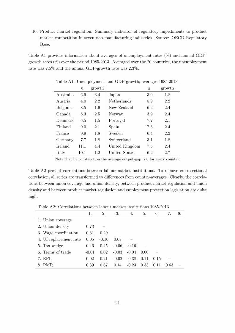
Table A1 provides information about averages of unemployment rates (%) and annual GDP-
growth rates (%) over the period 1985-2013. Averaged over the 20 countries, the unemployment
rate was 7.5% and the annual GDP-growth rate was 2.3%.
Table A1: Unemployment and GDP growth; averages 1985-2013
u growth u growth
Australia 6.9 3.4 Japan 3.9 1.8
Austria 4.0 2.2 Netherlands 5.9 2.2
Belgium 8.5 1.9 New Zealand 6.2 2.4
Canada 8.3 2.5 Norway 3.9 2.4
Denmark 6.5 1.5 Portugal 7.7 2.1
Finland 9.0 2.1 Spain 17.3 2.4
France 9.9 1.8 Sweden 6.4 2.2
Germany 7.7 1.8 Switzerland 3.1 1.8
Ireland 11.1 4.4 United Kingdom 7.5 2.4
Italy 10.1 1.2 United States 6.2 2.7
Note that by construction the average output-gap is 0 for every country.
Table A2 present correlations between labour market institutions. To remove cross-sectional
correlation, all series are transformed to differences from country-averages. Clearly, the correla-
tions between union coverage and union density, between product market regulation and union
density and between product market regulation and employment protection legislation are quite
high.
Table A2: Correlations between labour market institutions 1985-2013
1. 2. 3. 4. 5. 6. 7. 8.
1. Union coverage –
2. Union density 0.73 –
3. Wage coordination 0.31 0.29 –
4. UI replacement rate 0.05 -0.10 0.08 –
5. Tax wedge 0.46 0.45 -0.06 -0.16 –
6. Terms of trade -0.01 0.02 -0.03 -0.04 0.00 –
7. EPL 0.02 0.21 -0.02 -0.38 0.11 0.15 –
8. PMR 0.39 0.67 0.14 -0.23 0.33 0.11 0.63 –
21

Appendix B: Sensitivity analysis
B1: Adding a common factor
As a further check on the robustness of our results, we also introduced an additional common
factor into the Okun model:
uit = αi + βxit + φ(yit − y∗it) + κFt + eit (7)
with κ as additional parameter and Ft = Ft−1+νt. That is the equilibrium unemployment rates
are driven by labour market institutions and a common (global) latent variable. Preliminary
factor analysis using a principle components approach showed that the first principle component
accounts for around 40% of the variation of unemployment rate in the panel and it needs at
least 5 factors to account for about 90% of the variations. The results with a common factor
are shown Table B1. This table compares the parameter estimates of our baseline model where
column (1) replicates column (4) of Table 3 while column (2) present the parameter estimates
of the common factor approach.
Table B1: Adding a common factor
Baseline Common factor
GDP-gap 0.47 (0.00) 0.41 (0.00)
GDP-gap*share temp 0.05 (0.00) 0.03 (0.00)
Union density 0.06 (0.00) 0.01 (0.36)
Wage coordination -0.65 (0.00) -0.70 (0.00)
UI Replacement rate 0.04 (0.01) 0.06 (0.04)
Tax wedge 0.14 (0.00) 0.14 (0.00)
Terms of trade -0.06 (0.00) -0.06 (0.01)
Common factor 0.46 (0.00)
Constant 7.51 (0.00) 7.51 (0.00)
Note: p-values in parentheses
From a comparison of the parameter estimates in both columns, it is clear that some of the
parameter estimates are affected but with the exception of union density the parameter estimates
are not quantitatively different from each other. It would seem that the common factor is mainly
picking up the effect of union density. Since our aim is to be explicit about labour market
institutions, we have opted to concentrate on the model with the union density variable rather
than the one with the common (global) factor.
B2: Product market regulation
By way of sensitivity analysis we introduced an indicator for product market regulations as
additional explanatory variable (see also Appendix A). The results are shown in Table B2.
22

Table B2: Introducing Product Market Regulations
Variable (1) (2)
GDP-gap 0.48 (0.00) 0.48 (0.00)
Union density 0.00 (0.95)
Wage coordination -0.63 (0.00) -0.63 (0.00)
UI replacement rate 0.06 (0.00) 0.05 (0.00)
Tax wedge 0.14 (0.00) 0.14 (0.00)
Terms of trade -0.07 (0.00) -0.07 (0.00)
PMR 0.36 (0.00) 0.36 (0.00)
Constant 7.50 (0.00) 7.50 (0.00)
Note: p-values in parentheses
Product market regulations have a significant positive effect on the unemployment rate. How-
ever, now union density becomes insignificant. If we remove union density the effect of product
market regulations remains significantly positive. As shown in Table A2 product market reg-
ulation and union density are highly correlated. This correlation could arise because in many
countries over time PMR has been reduced at the same time as union density also dropped.
For illustrative purposes Table B3 shows estimates of the Okun relationship by age and gender
when we remove union density as explanatory variable and introduce PMR instead.
Table B3: Estimates by age and gender with PMR
Males Females
15-24 25-54 55-64 15-24 25-54 55-64
GDP-gap 1.07 (0.00) 0.52 (0.00) 0.46 (0.00) 0.70 (0.00) 0.30 (0.00) 0.24 (0.00)
GDP-gap*share temp 0.03 (0.00) 0.07 (0.00) 0.03 (0.19) 0.02 (0.02) 0.06 (0.00) -0.01 (0.48)
Wage coordination -0.65 (0.00) -0.22 (0.01) -0.25 (0.01) -0.87 (0.00) -0.57 (0.00) -0.18 (0.01)
UI Replacement rate -0.01 (0.84) 0.07 (0.00) 0.06 (0.01) -0.03 (0.25) 0.07 (0.01) 0.05 (0.01)
Tax wedge 0.07 (0.12) 0.12 (0.00) 0.05 (0.01) 0.11 (0.01) 0.14 (0.00) 0.08 (0.01)
Terms of trade -0.10 (0.00) -0.07 (0.02) -0.05 (0.00) -0.05 (0.02) -0.04 (0.00) -0.03 (0.00)
PMR -0.71 (0.00) -0.11 (0.04) 0.07 (0.05) 0.22 (0.07) 0.63 (0.00) 0.08 (0.05)
Constant 15.06 (0.00) 5.91 (0.00) 5.68 (0.00) 15.78 (0.00) 7.20 (0.00) 4.96 (0.00)
Note: p-values in parentheses
Now, we find that that PMR has significant negative effects on the unemployment rate of
young and prime age men. This is an odd result. Since these groups make up such a large
proportion of the total labour force, the finding that PMR has significant negative effects on
the unemployment rate of young and prime age men strengthens the case against including
PMR in the ‘aggregate model’. We think that the effect of PMR is actually is picking up the
effect of union density going down.
B3: Retirement ages
As a final sensitivity analysis we include the average age of retirement in the Okun relationship
for older workers. We do not have the average age of retirement in the main model because
this variable is potentially endogenous. After all, it could be that retirement age is reduced to
23

reduce unemployment rates of old workers. The parameter estimates shown in Table B4 indicate
that the average retirement age has a significant positive effect on the unemployment rate of
older workers. This would imply that an increase in retirement age increases unemployment
rates of old workers. Leaving aside the endogeneity issue this suggests that an increase in
retirement age stops some workers to make a transition to out of the labour force. Instead,
these workers become unemployed. However, the other parameter estimates are hardly affected
by the inclusion of this variable.
Table B4: Additional estimates workers aged 55-64
Males Females
GDP-gap 0.46 (0.00) 0.25 (0.00)
GDP-gap*share temp 0.02 (0.36) -0.02 (0.38)
Union density 0.05 (0.00) 0.04 (0.00)
Wage coordination -0.41 (0.00) -0.31 (0.00)
UI Replacement rate 0.08 (0.00) 0.06 (0.00)
Tax wedge 0.05 (0.00) 0.08 (0.00)
Terms of trade -0.05 (0.00) -0.03 (0.00)
Retirement age 0.17 (0.05) 0.10 (0.04)
Constant 5.70 (0.00) 4.96 (0.00)
Note: p-values in parentheses
24

Table 1: Okun relationship – 1985-2013
u∗ 7.50 (0.00)GDP-gap 0.54 (0.00)u∗jAustralia 6.89 (0.00) Japan 3.88 (0.00)Austria 4.04 (0.00) Netherlands 5.89 (0.00)Belgium 8.46 (0.00) New Zealand 6.21 (0.00)Canada 8.33 (0.00) Norway 3.93 (0.00)Denmark 6.47 (0.00) Portugal 7.71 (0.00)Finland 8.90 (0.00) Spain 17.31 (0.00)France 9.94 (0.00) Sweden 6.35 (0.00)Germany 7.73 (0.00) Switzerland 3.06 (0.00)Ireland 11.12 (0.00) United Kingdom 7.46 (0.00)Italy 10.14 (0.00) United States 6.23 (0.00)
Note: p-values in parentheses
Table 2: Symmetry and stability of the Okun relationship
Variable (1) (2) (3)u∗ 7.50 (0.00) 7.34 (0.00) 7.53 (0.00)GDP-gap 0.54 (0.00)GDP-gap pos 0.44 (0.00)GDP-gap neg 0.64 (0.00)GDP-gap pre GR 0.58 (0.00)GDP-gap post GR 0.37 (0.00)Wald testNo asymmetric effects 2.36 (0.12)No difference pre-post GR 4.16 (0.04)
Note: All estimates contain country fixed effects; the estimates in the first column are identical to the
ones presented in Table 1; p-values in parentheses
25

Table 3: Parameter estimates – including labour market institutions
Variable (1) (2) (3) (4) (5)GDP-gap 0.48 (0.00) 0.47 (0.00) 0.47 (0.00)GDP-gap pre GR 0.46 (0.00) 0.47 (0.00)GDP-gap post GR 0.53 (0.00) 0.48 (0.00)GDP-gap*share temp 0.05 (0.00) 0.05 (0.00) 0.04 (0.00)Union coverage 0.01 (0.33)Union density 0.05 (0.00) 0.06 (0.00) 0.06 (0.00) 0.06 (0.00) 0.04 (0.00)Wage coordination -0.76 (0.00) -0.68 (0.00) -0.65 (0.00) -0.65 (0.00) -0.90 (0.00)UI replacement rate 0.04 (0.02) 0.04 (0.01) 0.04 (0.01) 0.04 (0.00) 0.04 (0.00)Employment protection -0.01 (0.97)Tax wedge 0.13 (0.00) 0.14 (0.00) 0.14 (0.00) 0.14 (0.00) 0.22 (0.00)Terms of trade -0.06 (0.00) -0.06 (0.00) -0.06 (0.00) -0.06 (0.00) -0.04 (0.04)Constant 7.50 (0.00) 7.50 (0.00) 7.51 (0.00) 7.51 (0.00) 7.91 (0.00)
Note: Columns (1) to (4): 20 OECD countries; column (5): 15 European countries; all estimates
contain country fixed effects; p-values in parentheses. Column (2): the Wald test that pre-post Okun
coefficients are not statistically different from each other: 0.561 (0.454)
26

Table 4: Country-specific unemployment rates by age and gender;average 1985-2013 (%)
Women Men15-24 25-54 55-64 15-24 25-54 55-64
Australia 12.7 5.5 3.4 14.0 5.3 6.3Austria 7.6 4.1 3.1 7.3 3.5 4.2Belgium 21.7 9.6 5.0 17.5 5.9 4.1Canada 12.3 7.1 6.5 15.6 7.3 7.1Denmark 10.4 6.5 6.0 9.9 5.1 5.2Finland 18.6 7.0 8.6 18.7 7.5 9.2France 24.6 10.2 6.7 21.0 7.3 6.7Germany 8.5 7.8 10.8 9.3 6.7 9.5Ireland 16.5 9.2 5.7 20.5 10.5 6.9Italy 34.9 11.0 3.3 25.9 5.7 3.6Japan 6.5 3.6 2.6 7.7 3.1 5.1Netherlands 10.4 6.2 3.8 9.6 4.3 3.6New Zealand 13.0 4.9 3.1 13.8 4.8 3.9Norway 9.7 2.9 1.3 10.4 3.3 1.9Portugal 19.3 7.6 4.1 14.2 5.4 5.5Spain 39.2 19.5 10.0 29.7 12.2 10.2Sweden 15.2 4.8 4.1 16.5 5.3 5.3Switzerland 6.5 4.0 2.7 6.7 2.7 3.0United Kingdom 12.4 5.5 3.8 16.6 6.5 7.2United States 11.7 5.1 3.7 13.6 5.1 4.3
Average 15.8 7.2 5.0 15.1 5.9 5.7
Note that the data for Austria refer to the period from 1994 onwards, for New Zealand from 1986onwards and for Switzerland from 1991 onwards.
27

Table 5: Okun’s relationship by age and gender; 1985-2013
15-24 25-54 55-64Males Females Males Females Males Females
GDP-gap 1.14 (0.00) 0.76 (0.00) 0.56 (0.00) 0.36 (0.00) 0.45 (0.00) 0.26 (0.00)
u*
Australia 13.97 (0.00) 12.74 (0.00) 5.28 (0.00) 5.47 (0.00) 6.29 (0.00) 3.41 (0.00)Austria 7.18 (0.00) 7.52 (0.00) 3.46 (0.00) 4.03 (0.00) 4.19 (0.00) 3.04 (0.00)Belgium 17.48 (0.00) 21.68 (0.00) 5.93 (0.00) 9.56 (0.00) 4.11 (0.00) 4.96 (0.00)Canada 15.61 (0.00) 12.26 (0.00) 7.26 (0.00) 7.08 (0.00) 7.13 (0.00) 6.48 (0.00)Denmark 9.90 (0.00) 10.37 (0.00) 5.12 (0.00) 6.46 (0.00) 5.21 (0.00) 6.03 (0.00)Finland 18.66 (0.00) 18.56 (0.00) 7.50 (0.00) 6.97 (0.00) 9.23 (0.00) 8.61 (0.00)France 20.99 (0.00) 24.59 (0.00) 7.29 (0.00) 10.18 (0.00) 6.67 (0.00) 6.71 (0.00)Germany 9.35 (0.00) 8.53 (0.00) 6.70 (0.00) 7.81 (0.00) 9.52 (0.00) 10.80 (0.00)Ireland 20.49 (0.00) 16.48 (0.00) 10.48 (0.00) 9.22 (0.00) 6.94 (0.00) 5.66 (0.00)Italy 25.89 (0.00) 34.86 (0.00) 5.71 (0.00) 11.05 (0.00) 3.55 (0.00) 3.35 (0.00)Japan 7.70 (0.00) 6.48 (0.00) 3.13 (0.00) 3.57 (0.00) 5.06 (0.00) 2.56 (0.00)Netherlands 9.65 (0.00) 10.35 (0.00) 4.33 (0.00) 6.19 (0.00) 3.58 (0.00) 3.83 (0.00)New Zealand 13.79 (0.00) 12.96 (0.00) 4.74 (0.00) 4.90 (0.00) 3.92 (0.00) 3.09 (0.00)Norway 10.37 (0.00) 9.66 (0.00) 3.27 (0.00) 2.91 (0.00) 1.94 (0.00) 1.29 (0.00)Portugal 14.18 (0.00) 19.29 (0.00) 5.41 (0.00) 7.65 (0.00) 5.51 (0.00) 4.13 (0.00)Spain 29.66 (0.00) 39.21 (0.00) 12.16 (0.00) 19.53 (0.00) 10.19 (0.00) 10.03 (0.00)Sweden 16.54 (0.00) 15.15 (0.00) 5.27 (0.00) 4.77 (0.00) 5.35 (0.00) 4.14 (0.00)Switzerland 6.57 (0.00) 6.38 (0.00) 2.64 (0.00) 3.93 (0.00) 2.92 (0.00) 2.67 (0.00)United Kingdom 16.58 (0.00) 12.43 (0.00) 6.48 (0.00) 5.53 (0.00) 7.20 (0.00) 3.77 (0.00)United States 13.58 (0.00) 11.70 (0.00) 5.12 (0.00) 5.07 (0.00) 4.29 (0.00) 3.71 (0.00)
Note: p-values in parentheses
Table 6: Parameter estimates, effect institutions by age and gender
Males Females15-24 25-54 55-64 15-24 25-54 55-64
GDP-gap 1.05 (0.00) 0.52 (0.00) 0.45 (0.00) 0.70 (0.00) 0.29 (0.00) 0.23 (0.00)GDP-gap*share temp 0.03 (0.00) 0.07 (0.00) 0.03 (0.28) 0.02 (0.03) 0.05 (0.03) -0.01 (0.52)Union density -0.04 (0.14) 0.04 (0.00) 0.05 (0.00) 0.01 (0.83) 0.08 (0.00) 0.04 (0.00)Wage coordination -0.91 (0.00) -0.45 (0.00) -0.38 (0.00) -0.83 (0.00) -0.52 (0.00) -0.30 (0.00)UI replacement rate 0.03 (0.29) 0.09 (0.00) 0.06 (0.00) -0.04 (0.14) 0.03 (0.03) 0.05 (0.00)Tax wedge 0.05 (0.25) 0.09 (0.00) 0.03 (0.08) 0.12 (0.00) 0.15 (0.00) 0.07 (0.00)Terms of trade -0.10 (0.00) -0.07 (0.00) -0.05 (0.00) -0.05 (0.02) -0.03 (0.00) -0.03 (0.00)Constant 15.07 (0.00) 5.92 (0.00) 5.69 (0.00) 15.77 (0.00) 7.19 (0.00) 4.96 (0.00)
Note: All estimates contain country fixed effects; p-values in parentheses.
28

Figure 1: Unemployment rates and output gaps (inverse); 1985-2013
Note: Note: The solid lines are the actual unemployment rates (LHS) and the dashedlines are the (inverse) output gaps (RHS).
29

Figure 2: Labour market characteristics 1985 and 2013
a. Union Coverage (left) and Union Density (right)
b. Wage Coordination (left) and UI Replacement Rate (right)
c. Tax wedge (left) and Employment Protection Legislation (right)
30
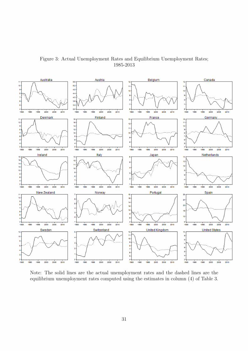
Figure 3: Actual Unemployment Rates and Equilibrium Unemployment Rates;1985-2013
Note: The solid lines are the actual unemployment rates and the dashed lines are theequilibrium unemployment rates computed using the estimates in column (4) of Table 3.
31

Figure 4: Unemployment rates and shares of temporary workers by age and gender –averaged over 20 countries; 1985-2013
a. Unemployment rates b. Shares of temporary workers
Figure 5: Equilibrium unemployment rates by country and age and by gender;1985-2013
a. Males b. Females
Note: based on parameter estimates from Table 5.
32
Recommended