1
MECH 221 FLUID MECHANICS(Fall 06/07)REVIEW
2
MECH 221 – Review
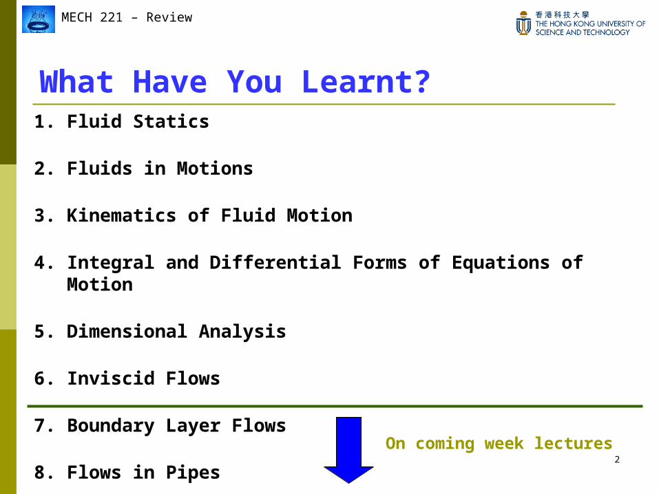
What Have You Learnt? 1. Fluid Statics
2. Fluids in Motions
3. Kinematics of Fluid Motion
4. Integral and Differential Forms of Equations of Motion
5. Dimensional Analysis
6. Inviscid Flows
7. Boundary Layer Flows
8. Flows in Pipes
9. Open Channel Flows
On coming week lectures
3
MECH 221 – Review
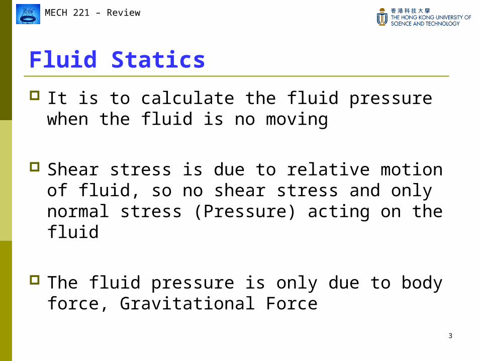
Fluid Statics It is to calculate the fluid pressure when the
fluid is no moving
Shear stress is due to relative motion of fluid, so no shear stress and only normal stress (Pressure) acting on the fluid
The fluid pressure is only due to body force, Gravitational Force
4
MECH 221 – Review
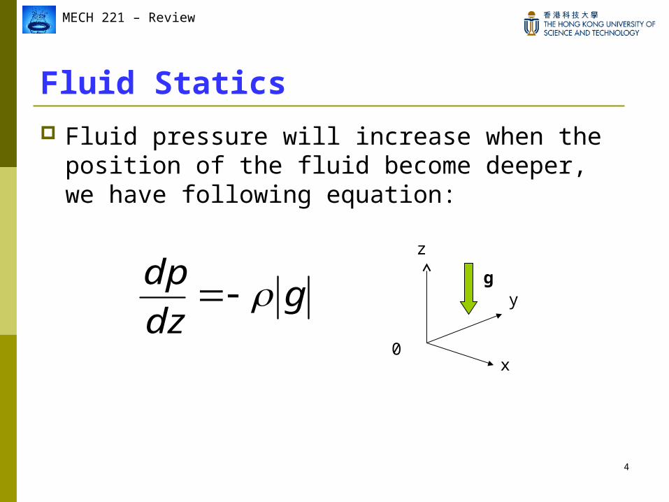
Fluid Statics Fluid pressure will increase when the position
of the fluid become deeper, we have following equation:
gdz
dp z
y
x
g
0
5
MECH 221 – Review
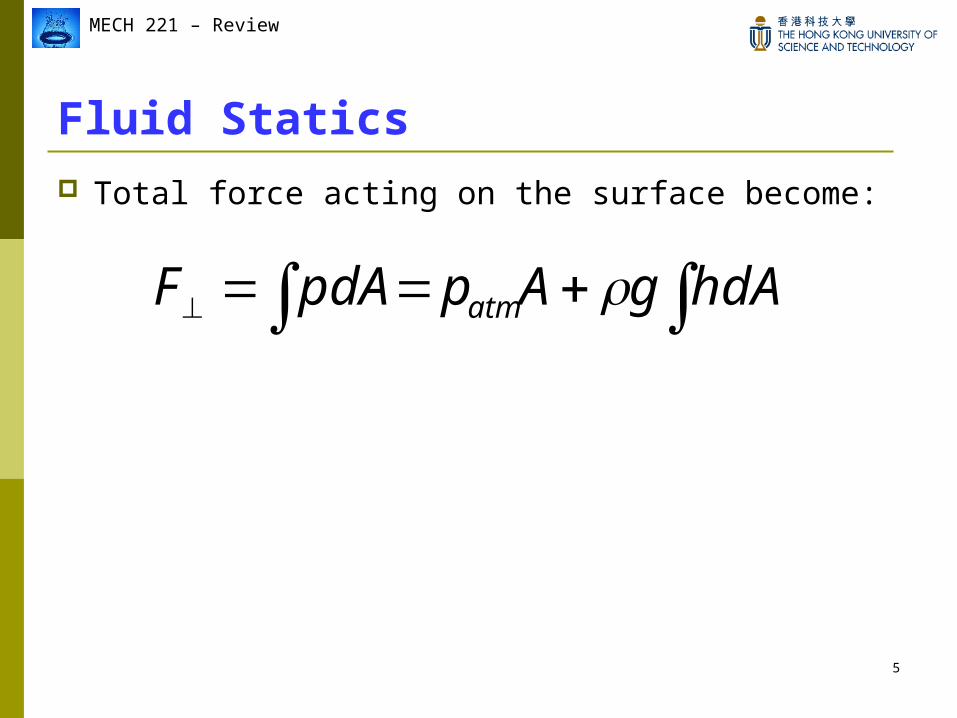
Fluid Statics Total force acting on the surface become:
hdAgAppdAF atm
6
MECH 221 – Review
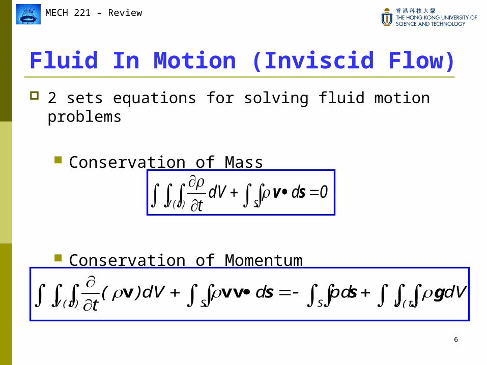
Fluid In Motion (Inviscid Flow) 2 sets equations for solving fluid motion problems
Conservation of Mass
Conservation of Momentum
dVpdddV)(t S )t(VS)t(V
gss vvv
0ddVt S)t(V
sv
7
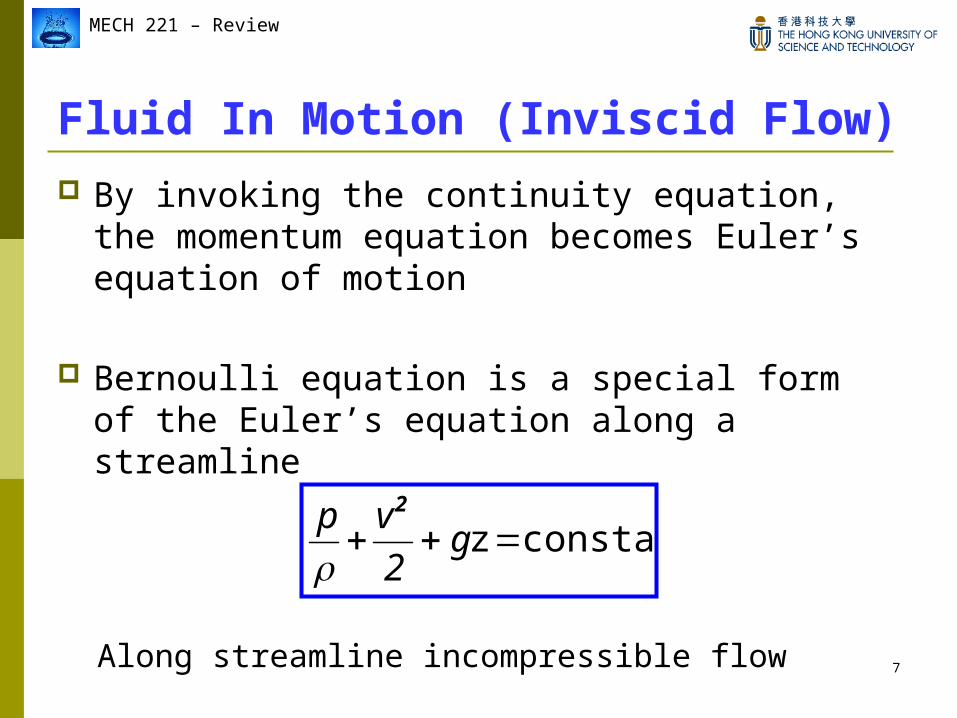
MECH 221 – Review
Fluid In Motion (Inviscid Flow) By invoking the continuity equation, the
momentum equation becomes Euler’s equation of motion
Bernoulli equation is a special form of the Euler’s equation along a streamline
constantz 2
g2
vp
Along streamline incompressible flow
8
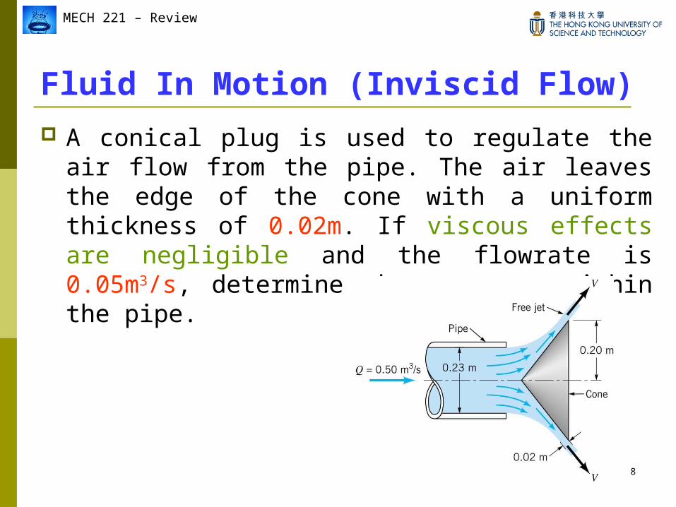
MECH 221 – Review
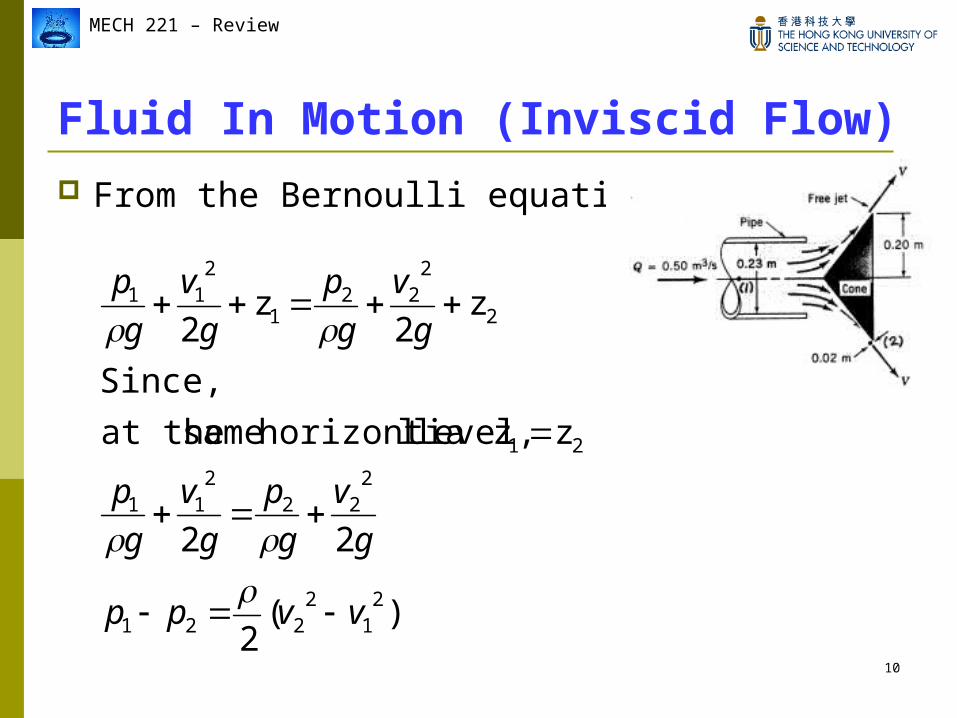
Fluid In Motion (Inviscid Flow) A conical plug is used to regulate the air flow
from the pipe. The air leaves the edge of the cone with a uniform thickness of 0.02m. If viscous effects are negligible and the flowrate is 0.05m3/s, determine the pressure within the pipe.
9
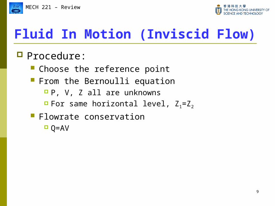
MECH 221 – Review
Fluid In Motion (Inviscid Flow) Procedure:
Choose the reference point From the Bernoulli equation
P, V, Z all are unknowns For same horizontal level, Z1=Z2
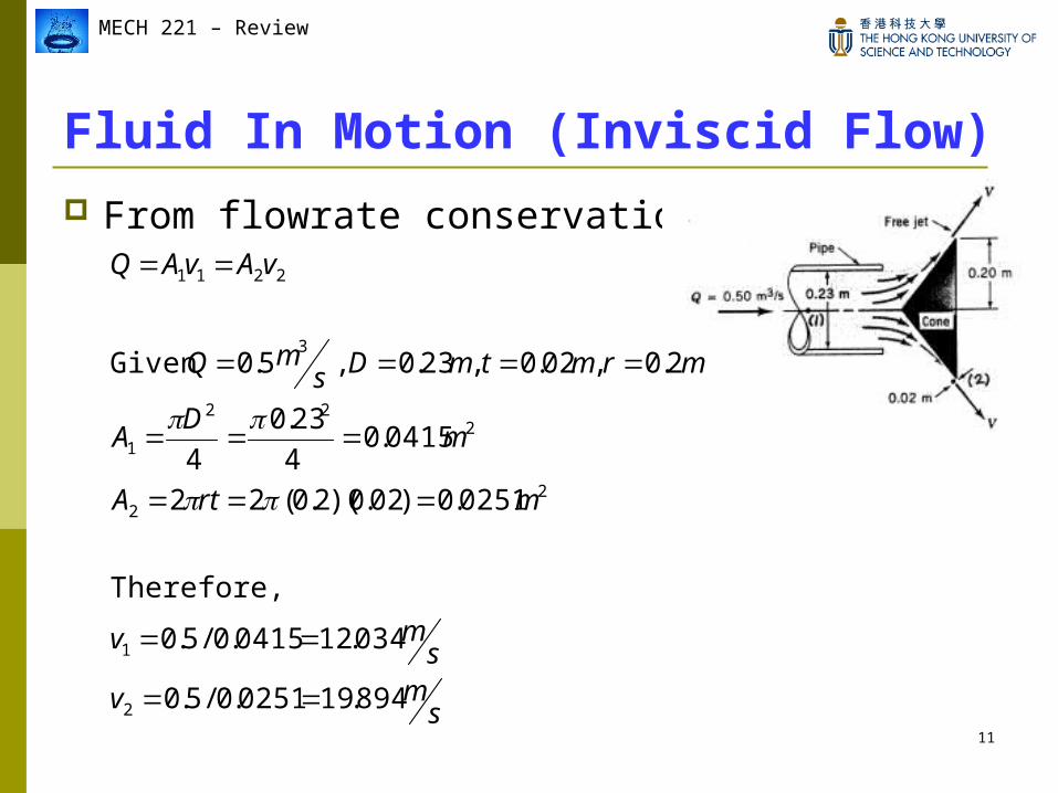
Flowrate conservation Q=AV
10
MECH 221 – Review
Fluid In Motion (Inviscid Flow) From the Bernoulli equation,
)(2
2
2
zz level, lhorizontia same at the
Since,
z 2
z 2
21
2221
222
211
21
2
222
1
211
vvpp
g
v
g
p
g
v
g
p
g
v
g
p
g
v
g
p
11
MECH 221 – Review
Fluid In Motion (Inviscid Flow) From flowrate conservation,
smv
smv
mrtA
mD
A
mrmtmDsmQ
vAvAQ
894.190251.0/5.0
034.120415.0/5.0
Therefore,
0251.0)02.0)(2.0(22
0415.04
23.0
4
2.0,02.0 ,23.0 ,5.0Given
2
1
22
222
1
3
2211
12
MECH 221 – Review
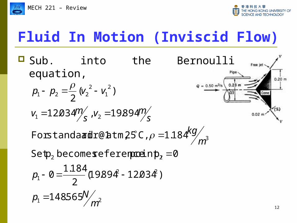
Fluid In Motion (Inviscid Flow)
21
221
22
3
21
21
2221
565.148
)034.12894.19(2
184.10
0p point, reference becomes pSet
184.1 C,25 atm, air@1 standardFor
894.19 ,034.12
)(2
mNp
p
mkg
smvs
mv
vvpp
Sub. into the Bernoulli equation,
13
MECH 221 – Review
Fluid In Motion (Viscous Flow) In the mentioned fluid motion is inviscid
flows, only pressure forces act on the fluid since the viscous forces (stress) were neglected
With the viscous stress, the total stress on the fluid is the sum of pressure stress ( ) and viscous stress ( ) given by:τ
pσ
τ pσσ

14
MECH 221 – Review
Fluid In Motion (Viscous Flow) The substitution of the viscous stress into the
momentum equations leads to:
These equations are also named as the Navier-Stokes equations
bτ
)()( p)(t
vvv
15
MECH 221 – Review
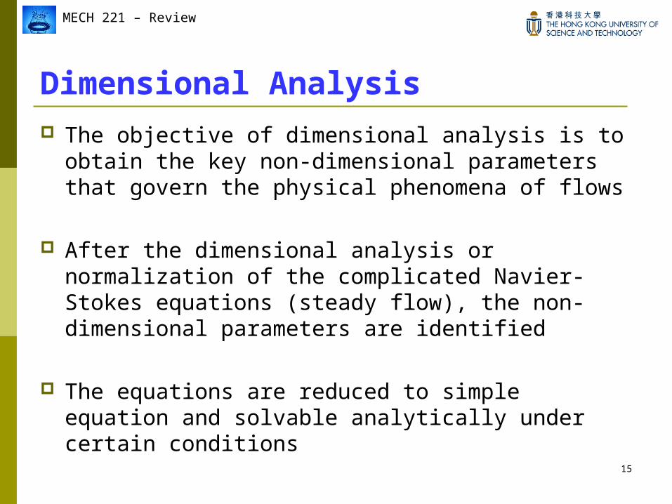
Dimensional Analysis The objective of dimensional analysis is to obtain
the key non-dimensional parameters that govern the physical phenomena of flows
After the dimensional analysis or normalization of the complicated Navier-Stokes equations (steady flow), the non-dimensional parameters are identified
The equations are reduced to simple equation and solvable analytically under certain conditions
16
MECH 221 – Review
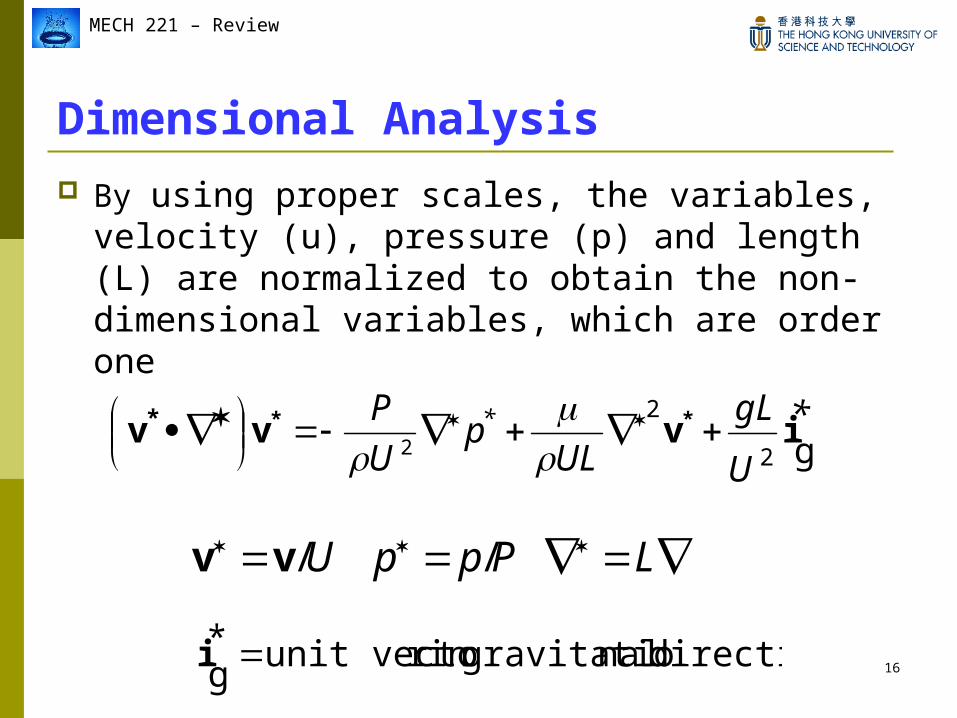
Dimensional Analysis By using proper scales, the variables, velocity
(u), pressure (p) and length (L) are normalized to obtain the non-dimensional variables, which are order one
*
U
gL
ULp
U
P *
g2
2
2ivvv ***
L Ppp U / /vv
direction nalgravitatio inr unit vecto *gi
17
MECH 221 – Review
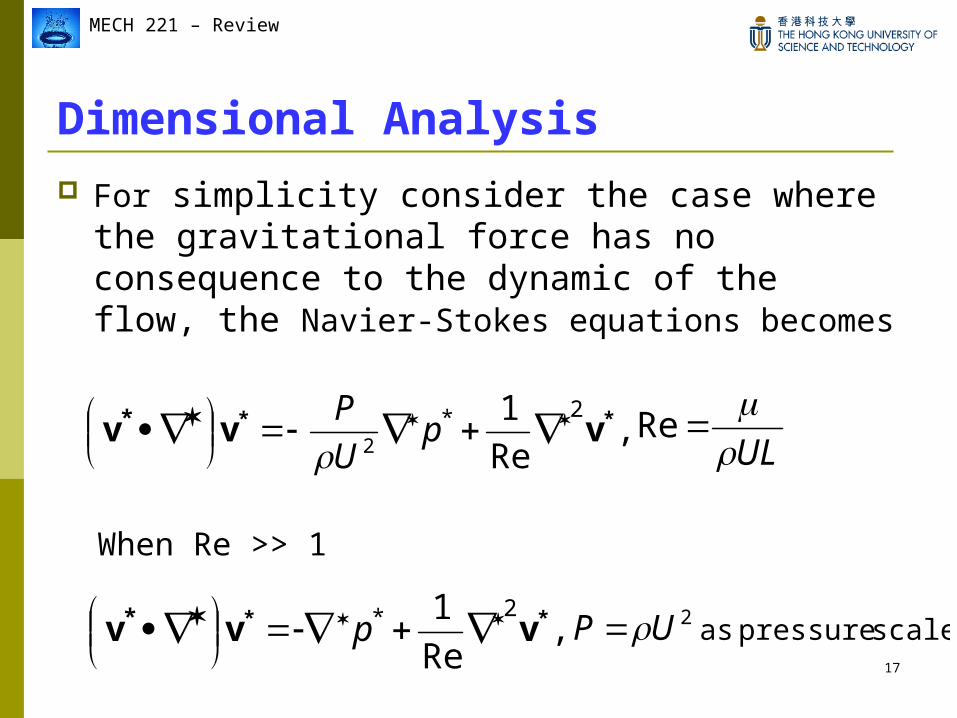
Dimensional Analysis For simplicity consider the case where the
gravitational force has no consequence to the dynamic of the flow, the Navier-Stokes equations becomes
UL
Re
,Re
1 2*2
** vvv*
p
U
P
,Re
1 2* ** vvv*
p
When Re >> 1
scale pressure as 2UP
18
MECH 221 – Review
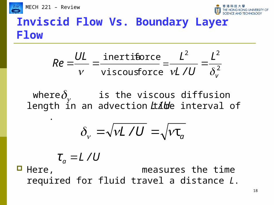
Inviscid Flow Vs. Boundary Layer Flow
where is the viscous diffusion length in an advection time interval of .
Here, measures the time required for fluid travel a distance L.
2
22
v
L
U/L
LULRe
force viscous
force inertia
U/L
U/Laτ
aU/L τ
19
MECH 221 – Review
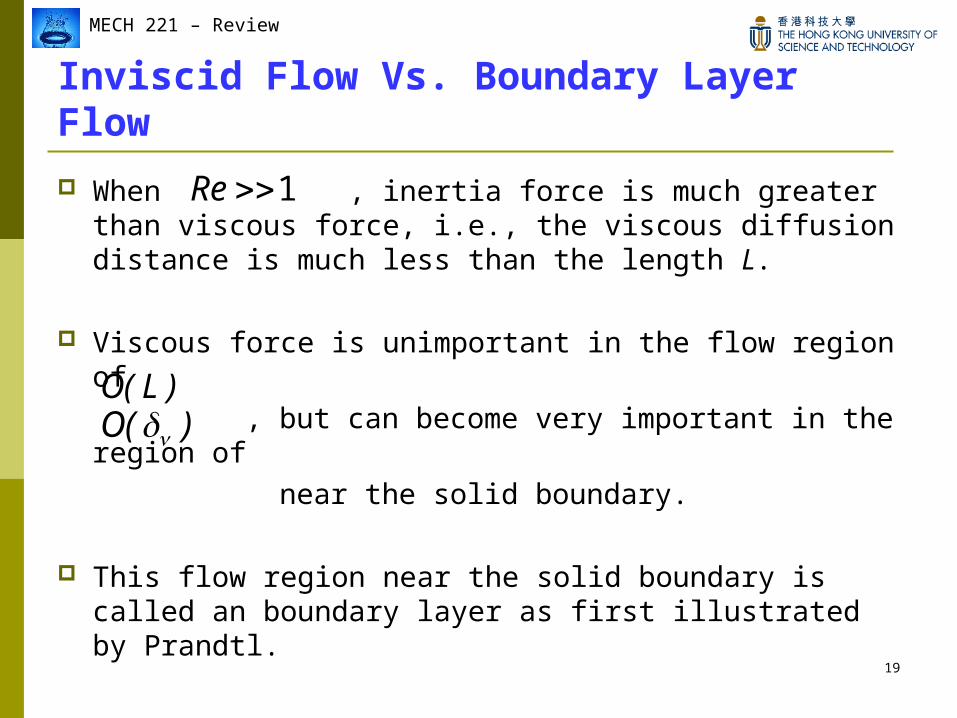
Inviscid Flow Vs. Boundary Layer Flow
When , inertia force is much greater than viscous force, i.e., the viscous diffusion distance is much less than the length L.
Viscous force is unimportant in the flow region of , but can become very important in the region of
near the solid boundary.
This flow region near the solid boundary is called an boundary layer as first illustrated by Prandtl.
1Re
)(O )L(O
20
MECH 221 – Review
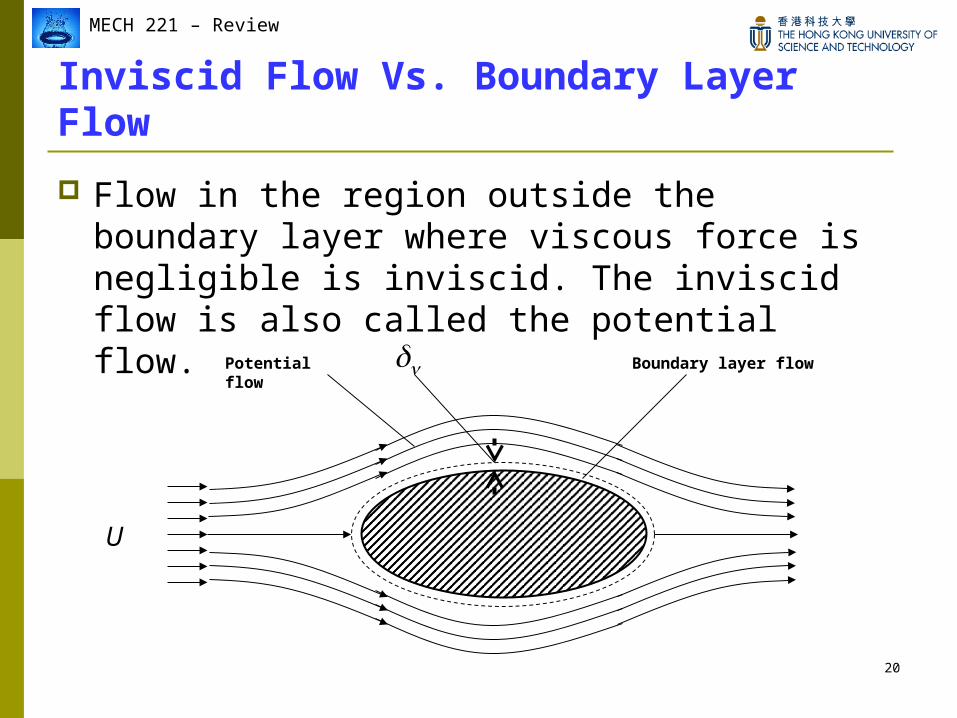
Inviscid Flow Vs. Boundary Layer Flow
Flow in the region outside the boundary layer where viscous force is negligible is inviscid. The inviscid flow is also called the potential flow.
U
Boundary layer flowPotential flow
21
MECH 221 – Review
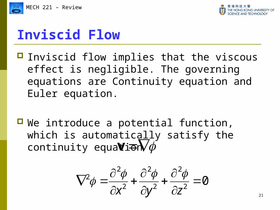
Inviscid Flow Inviscid flow implies that the viscous effect is
negligible. The governing equations are Continuity equation and Euler equation.
We introduce a potential function, which is automatically satisfy the continuity equation
v
02
2
2
2
2
22
zyx
22
MECH 221 – Review
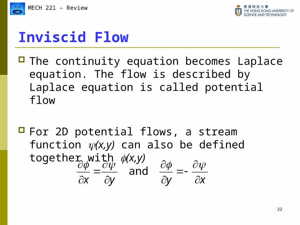
Inviscid Flow The continuity equation becomes Laplace
equation. The flow is described by Laplace equation is called potential flow
For 2D potential flows, a stream function (x,y) can also be defined together with (x,y)
xyyx
and
23
MECH 221 – Review
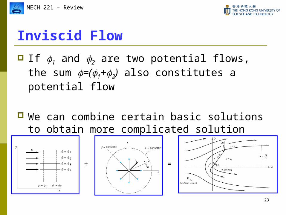
Inviscid Flow
If 1 and 2 are two potential flows, the sum =(1+2) also constitutes a potential flow
We can combine certain basic solutions to obtain more complicated solution
+ =
24
MECH 221 – Review
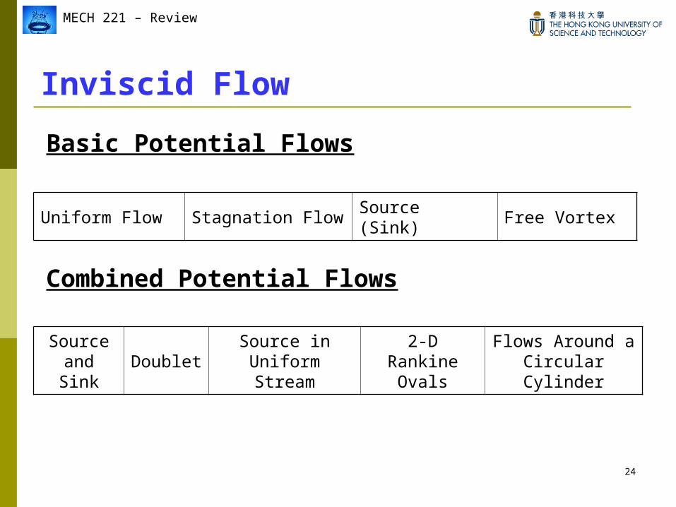
Inviscid Flow
Uniform Flow Stagnation Flow Source (Sink) Free Vortex
Source and Sink
DoubletSource in
Uniform Stream2-D Rankine
OvalsFlows Around a
Circular Cylinder
Basic Potential Flows
Combined Potential Flows
25
MECH 221 – Review
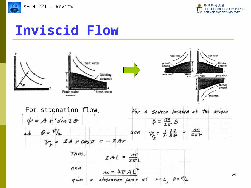
Inviscid Flow
For stagnation flow,
26
MECH 221 – Review
Boundary Layer Flow The thin layer adjacent to a solid boundary is
called the boundary layer and the flow inside the layer is called the boundary layer flow
Inside the thin layer the velocity of the fluid increases from zero at the wall (no slip) to the full value of corresponding potential flow.
27
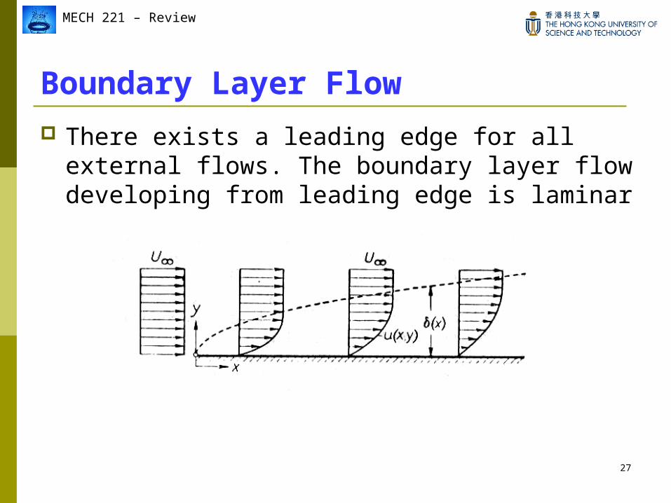
MECH 221 – Review
Boundary Layer Flow There exists a leading edge for all external
flows. The boundary layer flow developing from leading edge is laminar
28
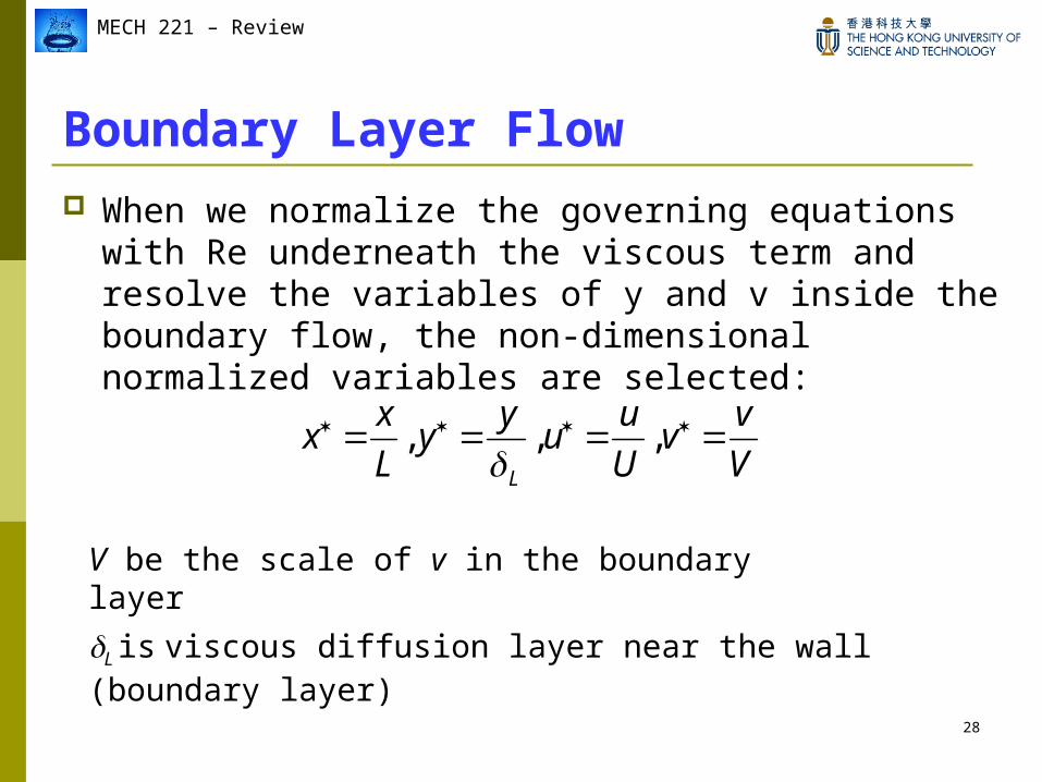
MECH 221 – Review
Boundary Layer Flow When we normalize the governing equations with
Re underneath the viscous term and resolve the variables of y and v inside the boundary flow, the non-dimensional normalized variables are selected:
V
vv
U
uu
yy
L
xx
L
,,,
V be the scale of v in the boundary layer
L is viscous diffusion layer near the wall (boundary layer)
29
MECH 221 – Review
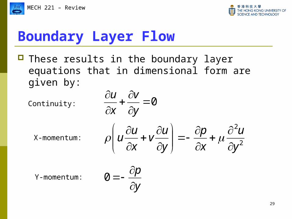
Boundary Layer Flow These results in the boundary layer equations that
in dimensional form are given by:
0
yx
vu
2
2
y
u
x
p
y
uv
x
uu
y
p
0
Continuity:
X-momentum:
Y-momentum:
30
MECH 221 – Review
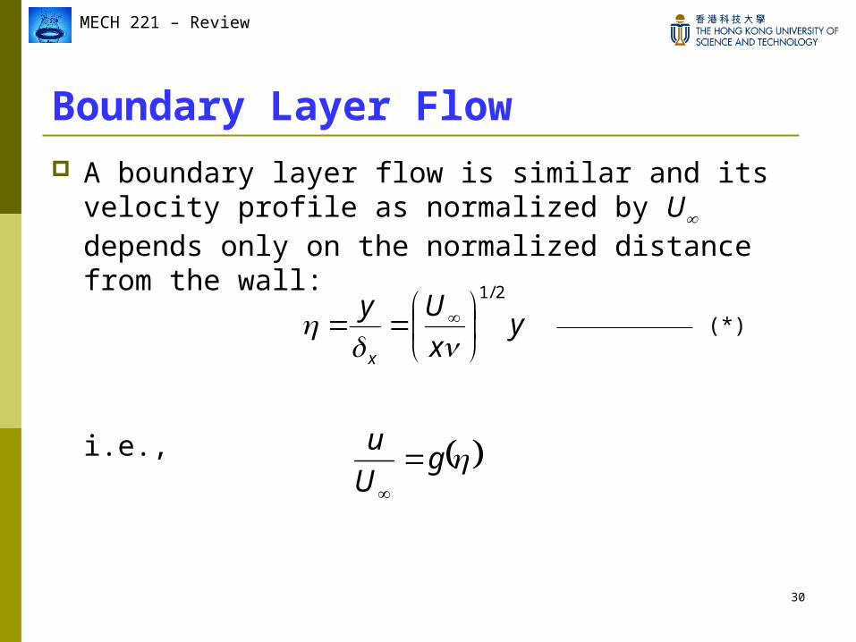
Boundary Layer Flow A boundary layer flow is similar and its velocity
profile as normalized by U depends only on the normalized distance from the wall:
i.e.,
yx
Uy
x
2/1
gU
u
(*)
31
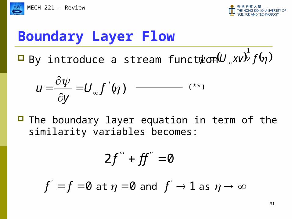
MECH 221 – Review
Boundary Layer Flow By introduce a stream function
The boundary layer equation in term of the similarity variables becomes:
)(' fU
yu
fxvU 2
1
f ff '' as and at 100
02 ''''' fff
(**)
32
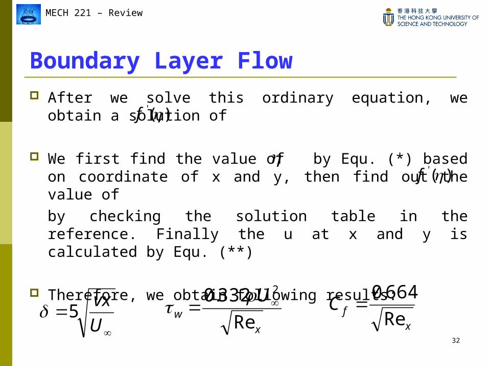
MECH 221 – Review
After we solve this ordinary equation, we obtain a solution of
We first find the value of by Equ. (*) based on coordinate of x and y, then find out the value of by checking the solution table in the reference. Finally the u at x and y is calculated by Equ. (**)
Therefore, we obtain following results:
Boundary Layer Flow
5
U
vx
)(' f
)(' f
x
w
U
Re
332.0 2
x
fCRe
664.0
33
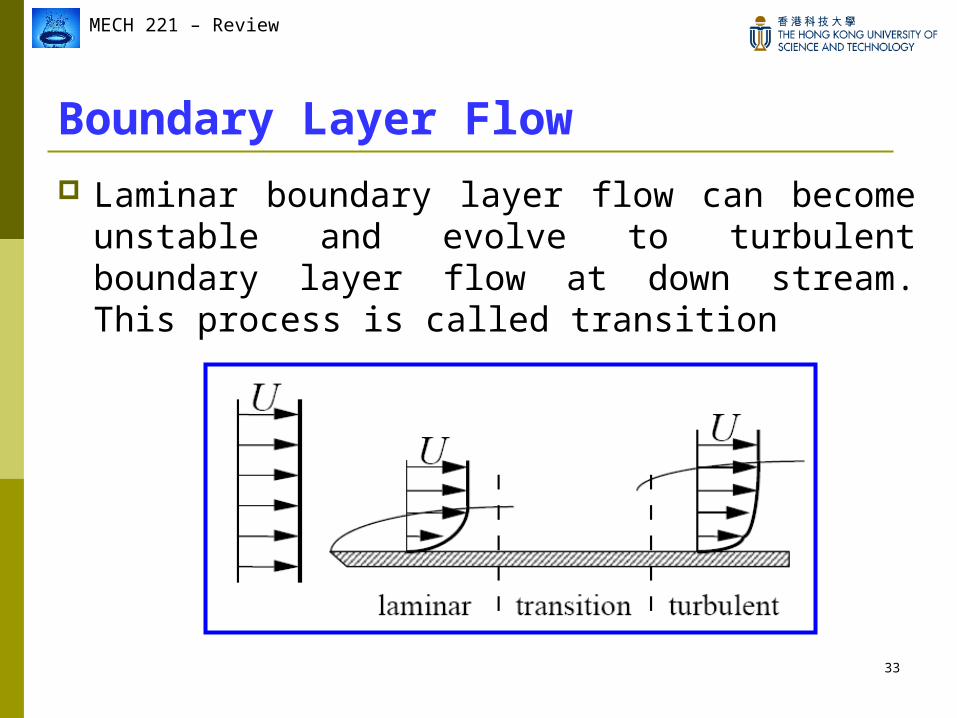
MECH 221 – Review
Boundary Layer Flow Laminar boundary layer flow can become
unstable and evolve to turbulent boundary layer flow at down stream. This process is called transition
34
MECH 221 – Review
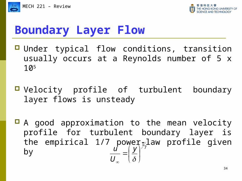
Boundary Layer Flow Under typical flow conditions, transition usually
occurs at a Reynolds number of 5 x 10⁵
Velocity profile of turbulent boundary layer flows is unsteady
A good approximation to the mean velocity profile for turbulent boundary layer is the empirical 1/7 power-law profile given by
71
y
U
u
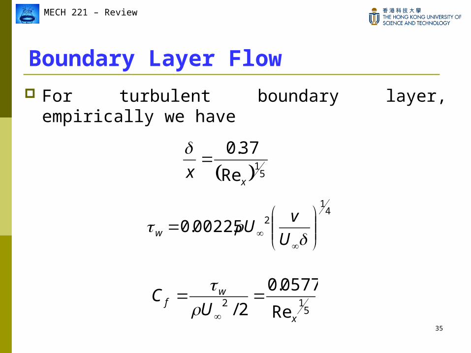
35
MECH 221 – Review
Boundary Layer Flow
51
Re
37.0
xx
512
Re
0577.0
2/x
wf
UC
41
200225.0
U
vUw
For turbulent boundary layer, empirically we have
36
MECH 221 – Review
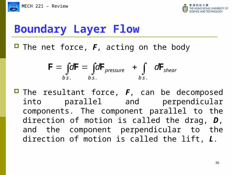
Boundary Layer Flow The net force, F, acting on the body
The resultant force, F, can be decomposed into parallel and perpendicular components. The component parallel to the direction of motion is called the drag, D, and the component perpendicular to the direction of motion is called the lift, L.
...... sb
shear
sb
pressure
sb
ddd FFFF
37
MECH 221 – Review
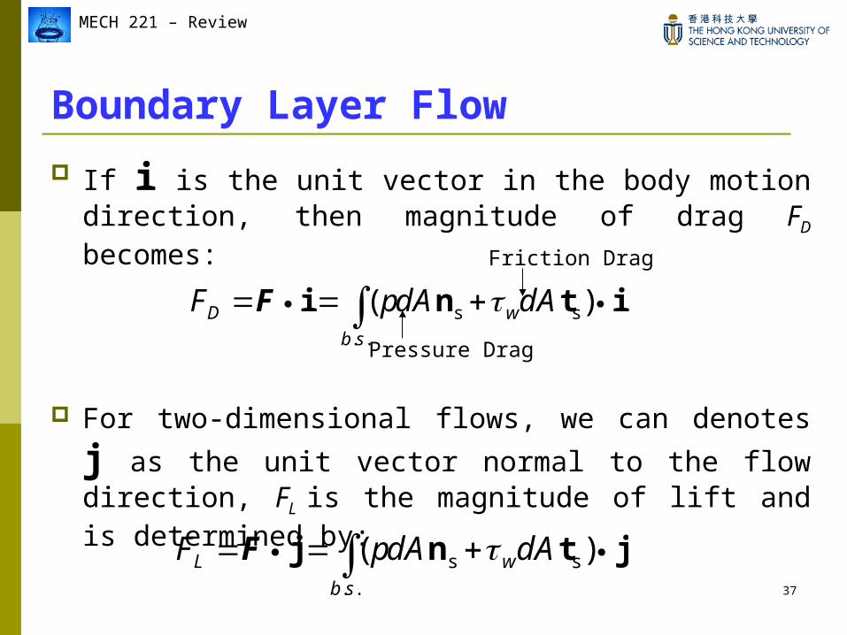
If i is the unit vector in the body motion direction, then magnitude of drag FD becomes:
For two-dimensional flows, we can denotes j as the unit vector normal to the flow direction, FL is the magnitude of lift and is determined by:
Boundary Layer Flow
)( ss
..
itni dAdApF w
sb
D F
jtnj )( ss
..
dAdApF w
sb
L F
Pressure Drag
Friction Drag
38
MECH 221 – Review
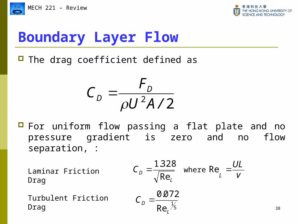
The drag coefficient defined as
For uniform flow passing a flat plate and no pressure gradient is zero and no flow separation, :
Boundary Layer Flow
22 /AU
FC D
D
Re
072.05
1
L
DC
vUL
CL
L
D ReRe
328.1 whereLaminar Friction Drag
Turbulent Friction Drag
39
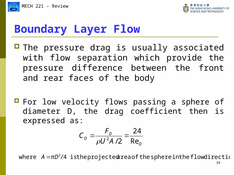
MECH 221 – Review
Boundary Layer Flow The pressure drag is usually associated with
flow separation which provide the pressure difference between the front and rear faces of the body
For low velocity flows passing a sphere of diameter D, the drag coefficient then is expressed as:
D
DD AU
FC
Re
24
2/2
direction flow the in sphere the of area projected the is where 42 /πDA
Recommended