Embed Size (px)
Citation preview
MECH 3492 Fluid Mechanics and Applications Univ. of Manitoba Fall Term, 2017
Chapter 2: Differential Analysis of Fluid Motion
Dr. Bing-Chen WangDept. of Mechanical Engineering
Univ. of Manitoba, Winnipeg, MB, R3T 5V6
1. Fluid Kinematics
1.1. Basic Fluid Motion and Deformation
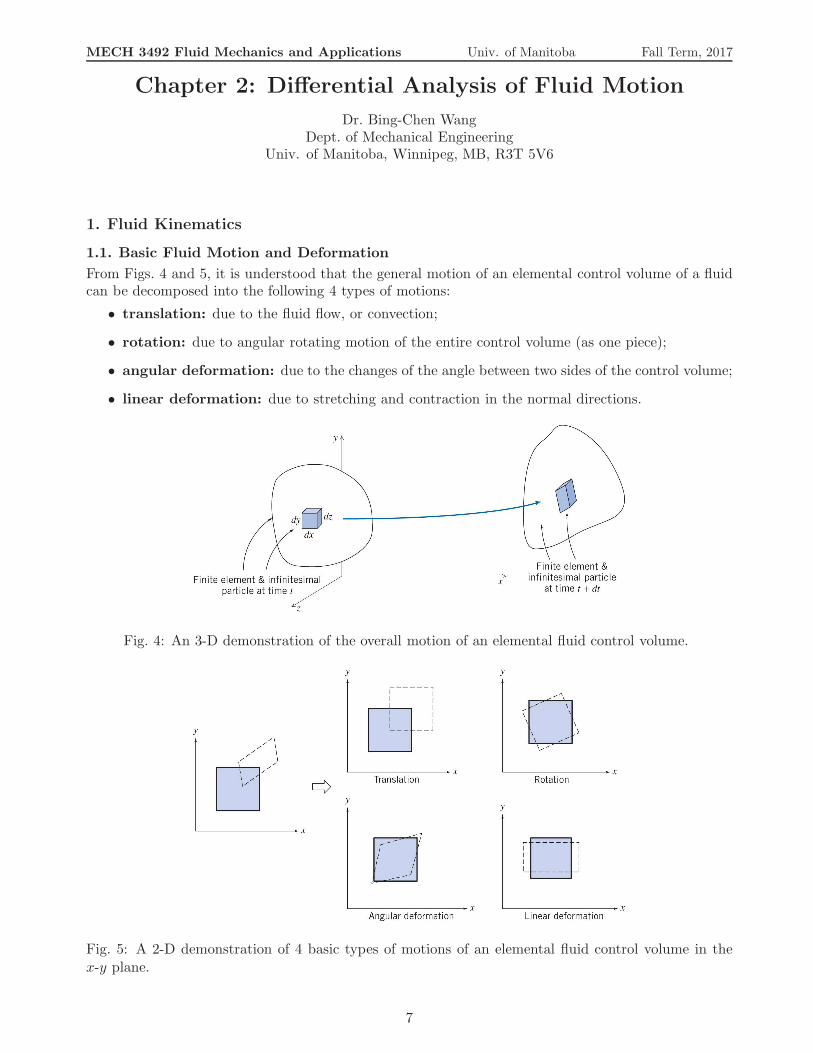
From Figs. 4 and 5, it is understood that the general motion of an elemental control volume of a fluidcan be decomposed into the following 4 types of motions:
• translation: due to the fluid flow, or convection;
• rotation: due to angular rotating motion of the entire control volume (as one piece);
• angular deformation: due to the changes of the angle between two sides of the control volume;
• linear deformation: due to stretching and contraction in the normal directions.
Fig. 4: An 3-D demonstration of the overall motion of an elemental fluid control volume.
Fig. 5: A 2-D demonstration of 4 basic types of motions of an elemental fluid control volume in thex-y plane.
7
MECH 3492 Fluid Mechanics and Applications Univ. of Manitoba Fall Term, 2017
1.2. Material Derivative
The material derivative (also called “substantial derivative”) of a physical quantity of a mate-rial/substance is defined as
D(·)
Dt︸ ︷︷ ︸
Rate of change
=∂(·)
∂t︸︷︷︸
Transient rate
+ V · ∇(·)︸ ︷︷ ︸
Convective rate
, (1)
The material derivative of a physical quantity (a scalar or a vector) describes its rate of change in aflow, which is caused by two factors: transient change (by itself over time), and interaction with theflow through convection. From this definition, the material derivative of temperature (T , a scalar) andthat of velocity (V, a vector) are expressed as:
DT
Dt=∂T
∂t+V · ∇T , (2)
DV
Dt︸︷︷︸
Totalacceleration
=∂V
∂t︸︷︷︸
Transientacceleration
+ V · ∇V︸ ︷︷ ︸
Convectiveacceleration
, (3)
respectively.
The material derivative of the velocity field V = [u, v, w] represent the total acceleration (rateof the change of velocity is acceleration) of the fluid. Obviously, the total acceleration of the fluid iscontributed by two parts: transient acceleration and convective acceleration. In a rectangular coordi-nate system, the total acceleration of the fluid can be expressed using components by expanding theterms in Eq. (3), i.e.
DV
Dt=∂V
∂t+ u
∂V
∂x+ v
∂V
∂y+ w
∂V
∂z, (4)
and further as
Du
Dt=∂u
∂t+ u
∂u
∂x+ v
∂u
∂y+ w
∂u
∂z
Dv
Dt=∂v
∂t+ u
∂v
∂x+ v
∂v
∂y+ w
∂v
∂z
Dw
Dt=∂w
∂t+ u
∂w
∂x+ v
∂w
∂y+ w
∂w
∂z
(5)
1.3. Fluid Rotation and Angular Deformation
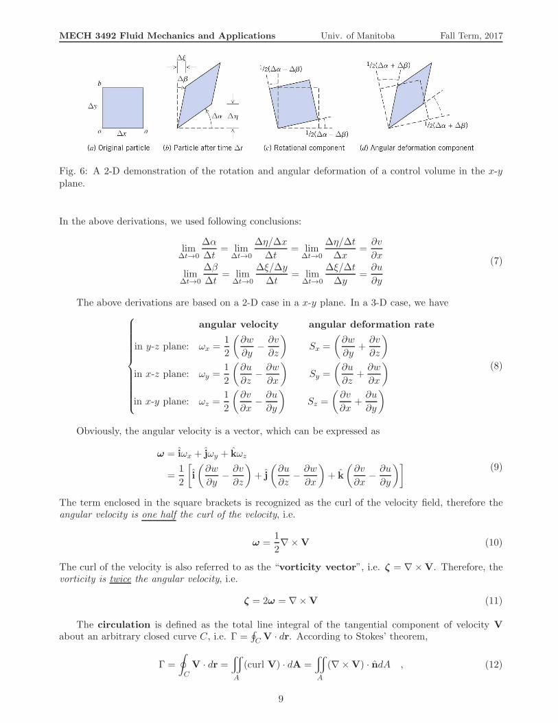
As explained in section 1.1, there four basic types of fluid motions, two of which relate to angularmotion, i.e. rotation and angular deformation. These two fluid motions are well-explained onpages 190-193 of the textbook (Pritchard, 2011). Figure 6 shows the rotation and angular deformationof a control volume in a 2-D plane. It can be reasoned from the figure that• the average rotation of the control volume is: ∆R = 1
2(∆α−∆β); and
• the angular deformation of the control volume is: ∆D = ∆α+∆β = 12(∆α+∆β) + 1
2(∆α+∆β).
Correspondingly, in the x-y plane, the angular velocity ωz and the angular deformation rateSz are determined as:
Angular velocity: ωz = lim∆t→0
∆R
∆t= lim
∆t→0
12(∆α−∆β)
∆t=
1
2
(∂v
∂x−∂u
∂y
)
,
Angular deformation rate: Sz = lim∆t→0
∆D
∆t= lim
∆t→0
(∆α+∆β)
∆t=
(∂v
∂x+∂u
∂y
)
.
(6)
8
MECH 3492 Fluid Mechanics and Applications Univ. of Manitoba Fall Term, 2017
Fig. 6: A 2-D demonstration of the rotation and angular deformation of a control volume in the x-yplane.
In the above derivations, we used following conclusions:
lim∆t→0
∆α
∆t= lim
∆t→0
∆η/∆x
∆t= lim
∆t→0
∆η/∆t
∆x=∂v
∂x
lim∆t→0
∆β
∆t= lim
∆t→0
∆ξ/∆y
∆t= lim
∆t→0
∆ξ/∆t
∆y=∂u
∂y
(7)
The above derivations are based on a 2-D case in a x-y plane. In a 3-D case, we have
angular velocity angular deformation rate
in y-z plane: ωx =1
2
(∂w
∂y−∂v
∂z
)
Sx =
(∂w
∂y+∂v
∂z
)
in x-z plane: ωy =1
2
(∂u
∂z−∂w
∂x
)
Sy =
(∂u
∂z+∂w
∂x
)
in x-y plane: ωz =1
2
(∂v
∂x−∂u
∂y
)
Sz =
(∂v
∂x+∂u
∂y
)
(8)
Obviously, the angular velocity is a vector, which can be expressed as
ω = iωx + jωy + kωz
=1
2
[
i
(∂w
∂y−∂v
∂z
)
+ j
(∂u
∂z−∂w
∂x
)
+ k
(∂v
∂x−∂u
∂y
)](9)
The term enclosed in the square brackets is recognized as the curl of the velocity field, therefore theangular velocity is one half the curl of the velocity, i.e.
ω =1
2∇×V (10)
The curl of the velocity is also referred to as the “vorticity vector”, i.e. ζ = ∇×V. Therefore, thevorticity is twice the angular velocity, i.e.
ζ = 2ω = ∇×V (11)
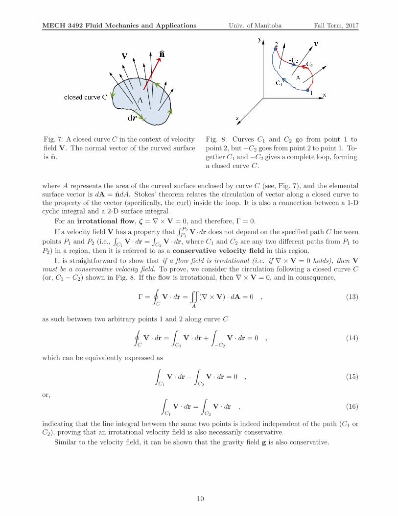
The circulation is defined as the total line integral of the tangential component of velocity Vabout an arbitrary closed curve C, i.e. Γ =
∮
CV · dr. According to Stokes’ theorem,
Γ =
∮
C
V · dr =x
A
(curl V) · dA =x
A
(∇×V) · ndA , (12)
9
MECH 3492 Fluid Mechanics and Applications Univ. of Manitoba Fall Term, 2017
Fig. 7: A closed curve C in the context of velocityfield V. The normal vector of the curved surfaceis n.
Fig. 8: Curves C1 and C2 go from point 1 topoint 2, but−C2 goes from point 2 to point 1. To-gether C1 and −C2 gives a complete loop, forminga closed curve C.
where A represents the area of the curved surface enclosed by curve C (see, Fig. 7), and the elementalsurface vector is dA = ndA. Stokes’ theorem relates the circulation of vector along a closed curve tothe property of the vector (specifically, the curl) inside the loop. It is also a connection between a 1-Dcyclic integral and a 2-D surface integral.
For an irrotational flow, ζ = ∇×V = 0, and therefore, Γ = 0.
If a velocity field V has a property that∫ P2
P1V ·dr does not depend on the specified path C between
points P1 and P2 (i.e.,∫
C1V · dr =
∫
C2V · dr, where C1 and C2 are any two different paths from P1 to
P2) in a region, then it is referred to as a conservative velocity field in this region.
It is straightforward to show that if a flow field is irrotational (i.e. if ∇ ×V = 0 holds), then Vmust be a conservative velocity field. To prove, we consider the circulation following a closed curve C(or, C1 −C2) shown in Fig. 8. If the flow is irrotational, then ∇×V = 0, and in consequence,
Γ =
∮
C
V · dr =x
A
(∇×V) · dA = 0 , (13)
as such between two arbitrary points 1 and 2 along curve C
∮
C
V · dr =
∫
C1
V · dr+
∫
−C2
V · dr = 0 , (14)
which can be equivalently expressed as
∫
C1
V · dr−
∫
C2
V · dr = 0 , (15)
or, ∫
C1
V · dr =
∫
C2
V · dr , (16)
indicating that the line integral between the same two points is indeed independent of the path (C1 orC2), proving that an irrotational velocity field is also necessarily conservative.
Similar to the velocity field, it can be shown that the gravity field g is also conservative.
10
MECH 3492 Fluid Mechanics and Applications Univ. of Manitoba Fall Term, 2017
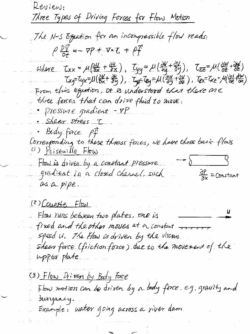
2. Governing Equations
2.1. Conservation Laws and Governing Equations
Fluid and Heat flows (or, thermal fluid flows) obey conservations laws. There are three conservationlaws involved in fluid mechanics and heat transfer:
• Mass Conservation,
• Momentum Conservation,
• Energy Conservation.
These three conservation laws result in three governing equations, which can be expressed in ei-ther integral forms or differential forms, so-called integral governing equations and differentialgoverning equations.
The integral governing equations are results of mass, momentum and energy conservations over afinite control volume (i.e., general balance over a finite-size domain), but the differential governingequations reflect exact mass, momentum and energy conservations at a point (or, exact balance at apoint enclosed in an infinitesimal control volume). As results of the three conservation laws, the set ofdifferential governing equations include:
• Mass Conservation Equation (also called “Continuity Equation”),
• Momentum Equation, (also called “Navier-Stokes Equation” if Stokes’ Hypothesis is acti-vated),
• Energy Equation.
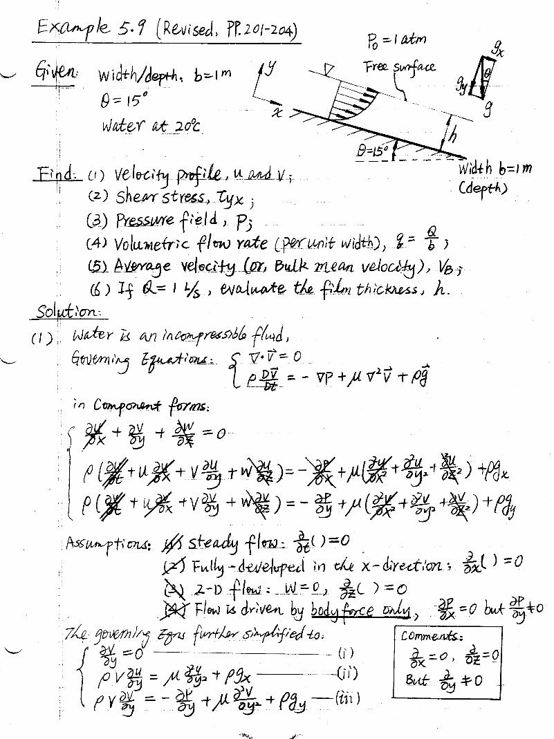
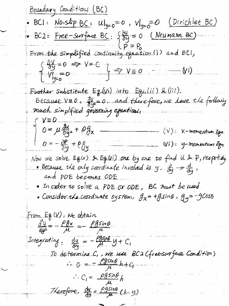
2.2. Governing Equations for an Incompressible Thermal Flow
For an incompressible thermal fluid flow, its density is constant, i.e. ρ = C. Therefore, any differen-tiation of density ρ with respect to time and space is zero, identically, i.e. dρ
dt≡ 0 and dρ
dx≡ 0. In the
context of an incompressible thermal flow, the three differential governing equations take the followingforms:
(1) Continuity Equation
∇ ·V = 0 , (17)
indicating that an incompressible flow is divergence free.∗
(2) Momentum Equation
From Newton’s second law, for a unit control volume of the fluid, the momentum equation reads:
ρDV
Dt︸ ︷︷ ︸
Rate of changein momentum
=∑
i
fi
︸ ︷︷ ︸
External forces
, (19)
∗It should be indicated that the general continuity equation for both compressible and incompressible flows reads:
∂ρ
∂t+∇ · (ρV) = 0 . (18)
In the special context of incompressible flow, this general continuity equation reduces to Eq. (17).
11
MECH 3492 Fluid Mechanics and Applications Univ. of Manitoba Fall Term, 2017
where DV
Dtis the total acceleration of the fluid, fi is an external force exerted on a unit control volume.†
The external forces exerted on the control volume include:• normal and shear stresses (represented by the stress tensor τ , see Eq. (4) and Fig. 2), and• body forces (such as the gravitational force and buoyancy).Therefore, the momentum equation that governs the flow motion reads
ρDV
Dt= ∇ · τ + ρf , (20)
which can be further expressed in component forms as
ρ
(∂u
∂t+ u
∂u
∂x+ v
∂u
∂y+ w
∂u
∂z
)
=
(∂σxx∂x
+∂τyx∂y
+∂τzx∂z
)
+ ρfx
ρ
(∂v
∂t+ u
∂v
∂x+ v
∂v
∂y+ w
∂v
∂z
)
=
(∂τxy∂x
+∂σyy∂y
+∂τzy∂z
)
+ ρfy
ρ
(∂w
∂t+ u
∂w
∂x+ v
∂w
∂y+w
∂w
∂z
)
=
(∂τxz∂x
+∂τyz∂y
+∂σzz∂z
)
+ ρfz .
(21)
For an incompressible flow, ∇ ·V = 0 and Stokes’ hypothesis assumes that
σxx = −p+ 2µ∂u
∂xσyy = −p+ 2µ
∂v
∂yσzz = −p+ 2µ
∂w
∂z
τxy = τyx = µ
(∂v
∂x+∂u
∂y
)
τyz = τzy = µ
(∂w
∂y+∂v
∂z
)
τzx = τxz = µ
(∂u
∂z+∂w
∂x
) (22)
where µ is the dynamic viscosity of the fluid. Stokes’ hypothesis builds a constitutive relationshipbetween stresses and velocity gradients for a Newtonian fluid.‡
By utilizing Stokes’ hypothesis (i.e., substituting Eq. (22) into Eq. (20)), the momentum equationbecomes:
ρDV
Dt= −∇p+ µ∇2V+ ρf . (23)
†Note that Newton’s second law reads: ma =∑
iFi. Here Fi is an external force, m = ρV is the mass, and V is the
volume. For a unit control volume, Newton’s second law becomes ρa =∑
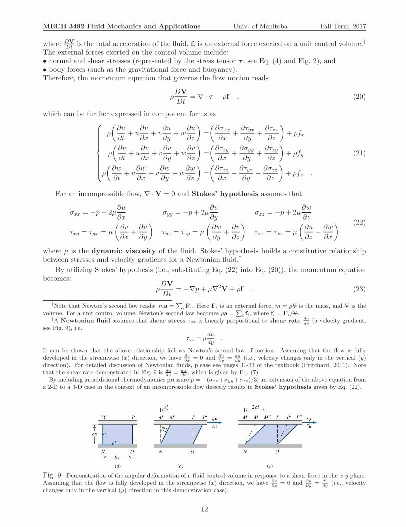
i fi, where fi = Fi/V.‡A Newtonian fluid assumes that shear stress τyx is linearly proportional to shear rate du
dy(a velocity gradient,
see Fig. 9), i.e.
τyx = µdu
dy.
It can be shown that the above relationship follows Newton’s second law of motion. Assuming that the flow is fullydeveloped in the streamwise (x) direction, we have ∂v
∂x= 0 and ∂u
∂y= du
dy(i.e., velocity changes only in the vertical (y)
direction). For detailed discussion of Newtonian fluids, please see pages 31-33 of the textbook (Pritchard, 2011). Notethat the shear rate demonstrated in Fig. 9 is du
dy= dα
dt, which is given by Eq. (7).
By including an additional thermodynamics pressure p = −(σxx+σyy+σzz)/3, an extension of the above equation froma 2-D to a 3-D case in the context of an incompressible flow directly results in Stokes’ hypothesis given by Eq. (22).
Fig. 9: Demonstration of the angular deformation of a fluid control volume in response to a shear force in the x-y plane.Assuming that the flow is fully developed in the streamwise (x) direction, we have ∂v
∂x= 0 and ∂u
∂y= du
dy(i.e., velocity
changes only in the vertical (y) direction in this demonstration case).
12
MECH 3492 Fluid Mechanics and Applications Univ. of Manitoba Fall Term, 2017
This form of the momentum equation (derived based on Stokes’ hypothesis) is referred to as the so-called “Navier-Stokes equation”, named after C. L. M. H. Navier (1785-1836) and Sir George G.Stokes (1819-1903).
Dividing both sides of Eq. (23) by ρ, we obtain:
DV
Dt= −
1
ρ∇p+ ν∇2V + f , (24)
where ν = µ/ρ is the kinematic viscosity of the fluid. If the gravitational force is the body force(i.e., f = g), the above equation becomes:
∂V
∂t︸︷︷︸
Transient term
+ V · ∇V︸ ︷︷ ︸
Convection
= −1
ρ∇p
︸ ︷︷ ︸
Pressure gradient
+ ν∇2V︸ ︷︷ ︸
Diffusion
+ g︸︷︷︸
Gravity
. (25)
The physical meaning of each term is annotated under the curly bracket.
(3) Thermal Energy Equation
DT
Dt= α∇2T + S , (26)
where S is a heat source/sink term, and α = kρCP
is molecular thermal diffusivity of the fluid. Herek is the thermal conductivity of the fluid and CP is the specific heat under a constant pressure. Thephysical meaning of the above equation can be explained as
∂T
∂t︸︷︷︸
Transient term
+ V · ∇T︸ ︷︷ ︸
Convection
= α∇2T︸ ︷︷ ︸
Diffusion
+ S︸︷︷︸
Source Term
. (27)
The above thermal energy equation is also called the “convection-diffusion equation” of a scalar,and it governs both heat conduction and heat convection. If the fluid is still (no flow motion is involved)or if the material is a solid, the convection term vanishes. Then, the above equation reduces to theheat conduction equation (for both solid and liquid), viz.
∂T
∂t= α∇2T + S . (28)
If the heat conduction process is steady state, then the transient term vanishes, and the above heatequation further reduces to
α∇2T + S = 0 . (29)
which is a Poisson’s equation, dominated by the molecular diffusion term α∇2T (also called the “con-duction term”).
13
MECH 3492 Fluid Mechanics and Applications Univ. of Manitoba Fall Term, 2017
SummaryFor an incompressible thermal fluid flow under the gravitational force, the set of three governingequations reads:
Continuity Equation: ∇ ·V = 0 ,
Momentum Equation:DV
Dt= −
1
ρ∇p+ ν∇2V+ g ,
Thermal Energy Equation:DT
Dt= α∇2T + S .
(30)
Note:
(1) If heat transfer is not involved, then the thermal energy equation is not needed. For a pure fluidsproblem, only two governing equations are needed: continuity and momentum equations.(2) The momentum and thermal energy equations can be considered as “transport equations” formomentum and thermal energy (indicated by temperature T ). In general, a transport equation for aphysical quantity (either a vector or a scalar) includes:
• material derivative (on the left hand side),• a diffusion term and an external source (or force) term (on the right hand side).
(3) The convection term is a consequence of flow motion at macro scales, but the diffusion term is dueto the molecular motions at micro scales (so-called “Brownian motion” of molecules).A weblink for Brownian motion: http://en.wikipedia.org/wiki/Brownian%5Fmotion(4) Convection V · ∇T is sensitive to the flow direction (because of V), but diffusion (α∇2T ) isa molecular behavior (determined by ν and α) and takes effects in all directions (i.e., diffusion isinsensitive to mean flow directions).
2.3. Governing Equations in Component Forms (for fluid flow only)
For an incompressible fluid flow under the gravitational force, the two governing equations (continuityand momentum equations) summarized in Eq. (30) are:
Continuity Equation: ∇ ·V = 0 ,
Momentum Equation: ρDV
Dt= −∇p+ µ∇2V + ρg ,
(31)
which can be further expanded using in component forms in both rectangular and cylindrical coordinatesystems as follows:
• Rectangular Coordinate System
Continuity Equation:∂u
∂x+∂v
∂y+∂w
∂z= 0 ,
Momentum Equation:
ρ
(∂u
∂t+ u
∂u
∂x+ v
∂u
∂y+ w
∂u
∂z
)
=−∂p
∂x+ µ
(∂2u
∂x2+∂2u
∂y2+∂2u
∂z2
)
+ ρgx
ρ
(∂v
∂t+ u
∂v
∂x+ v
∂v
∂y+w
∂v
∂z
)
=−∂p
∂y+ µ
(∂2v
∂x2+∂2v
∂y2+∂2v
∂z2
)
+ ρgy
ρ
(∂w
∂t+ u
∂w
∂x+ v
∂w
∂y+ w
∂w
∂z
)
=−∂p
∂z+ µ
(∂2w
∂x2+∂2w
∂y2+∂2w
∂z2
)
+ ρgz .
(32)
14
MECH 3492 Fluid Mechanics and Applications Univ. of Manitoba Fall Term, 2017
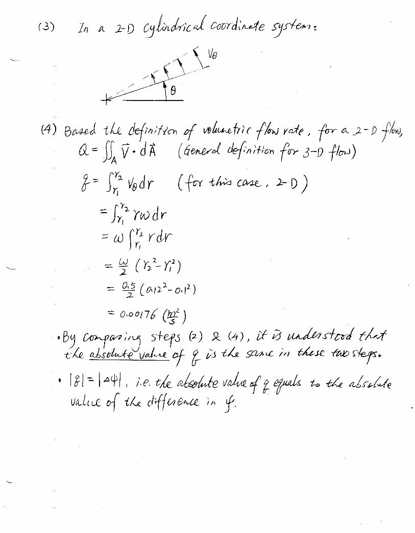
• Cylindrical Coordinate System
Continuity Equation:1
r
∂(rVr)
∂r+
1
r
∂Vθ∂θ
+∂Vz∂z
= 0 ,
Momentum Equation:
r-component:
ρ
(∂Vr∂t
+ Vr∂Vr∂r
+Vθr
∂Vr∂θ
−V 2θ
r+ Vz
∂Vr∂z
)
=
ρgr −∂p
∂r+ µ
{∂
∂r
[1
r
∂
∂r(rVr)
]
+1
r2∂2Vr∂θ2
−2
r2∂Vθ∂θ
+∂2Vr∂z2
}
θ-component:
ρ
(∂Vθ∂t
+ Vr∂Vθ∂r
+Vθr
∂Vθ∂θ
+VrVθr
+ Vz∂Vθ∂z
)
=
ρgθ−
1
r
∂p
∂θ+ µ
{∂
∂r
[1
r
∂
∂r(rVθ)
]
+1
r2∂2Vθ∂θ2
+2
r2∂Vr∂θ
+∂2Vθ∂z2
}
z-component:
ρ
(∂Vz∂t
+ Vr∂Vz∂r
+Vθr
∂Vz∂θ
+ Vz∂Vz∂z
)
=
ρgz −∂p
∂z+ µ
{1
r
∂
∂r
(
r∂Vz∂r
)
+1
r2∂2Vz∂θ2
+∂2Vz∂z2
}
.
(33)
REFERENCES
Pritchard, P. J. 2011, Fox and McDonald’s Introduction to Fluids Mechanics, 8th edition, Wiley, USA.
White, F. M. 2011, Fluid Mechanics, 7th edition, McGraw-Hill, New York, NY.
15
MECH 3492 Fluid Mechanics and Applications Univ. of Manitoba Fall Term, 2017
3. Stream Function
For a 2-D incompressible flow field V = iu+ jv, the continuity equation reads:
∂u
∂x+∂v
∂y= 0 . (34)
The stream function ψ = ψ(x, y) is defined such that
u ≡∂ψ
∂yand v ≡ −
∂ψ
∂x, (35)
with which, the continuity equation (34) reduces to a trivial form, i.e.
∂2ψ
∂x∂y−
∂2ψ
∂y∂x≡ 0 . (36)
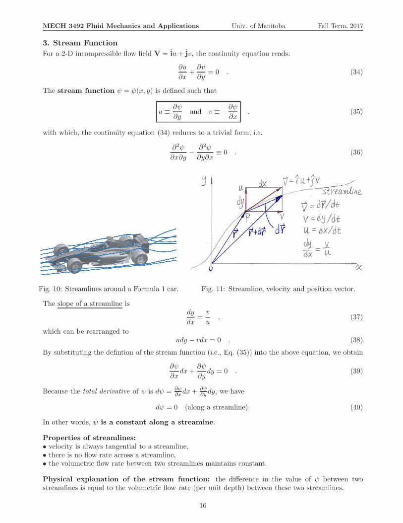
Fig. 10: Streamlines around a Formula 1 car. Fig. 11: Streamline, velocity and position vector.
The slope of a streamline isdy
dx=v
u, (37)
which can be rearranged toudy − vdx = 0 . (38)
By substituting the defintion of the stream function (i.e., Eq. (35)) into the above equation, we obtain
∂ψ
∂xdx+
∂ψ
∂ydy = 0 . (39)
Because the total derivative of ψ is dψ = ∂ψ∂xdx+ ∂ψ
∂ydy, we have
dψ = 0 (along a streamline). (40)
In other words, ψ is a constant along a streamine.
Properties of streamlines:• velocity is always tangential to a streamline,• there is no flow rate across a streamline,• the volumetric flow rate between two streamlines maintains constant.
Physical explanation of the stream function: the difference in the value of ψ between twostreamlines is equal to the volumetric flow rate (per unit depth) between these two streamlines.
16
MECH 3492 Fluid Mechanics and Applications Univ. of Manitoba Fall Term, 2017
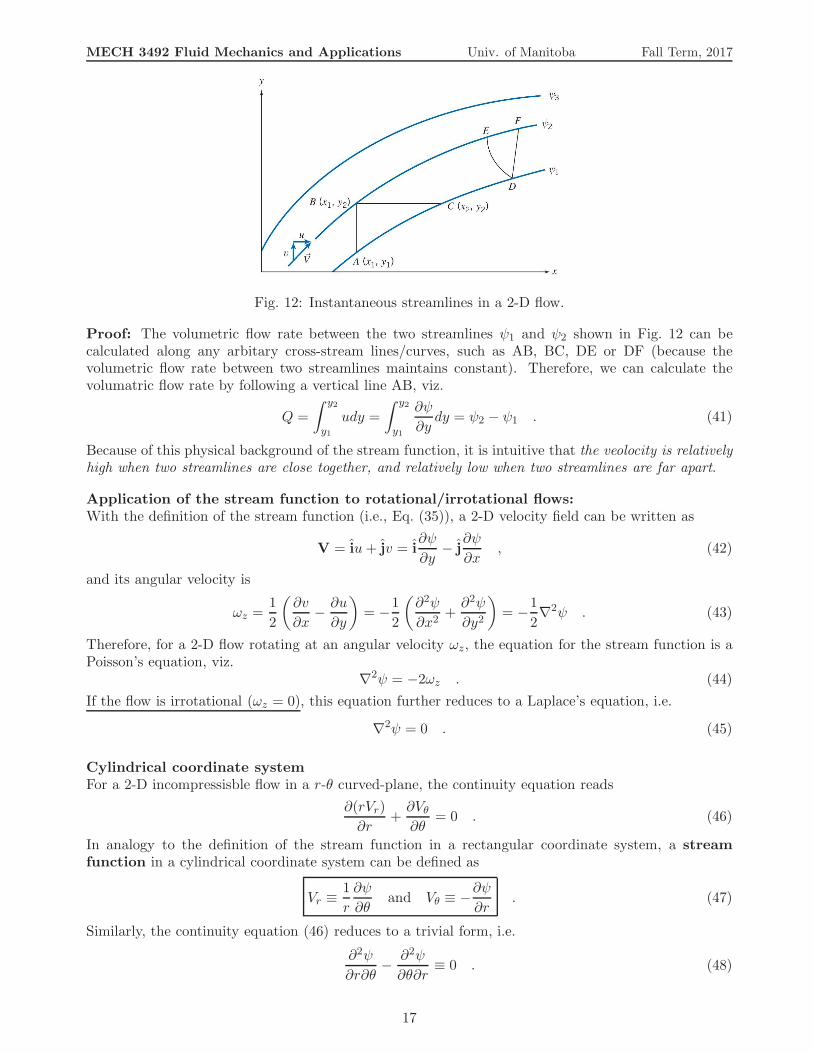
Fig. 12: Instantaneous streamlines in a 2-D flow.
Proof: The volumetric flow rate between the two streamlines ψ1 and ψ2 shown in Fig. 12 can becalculated along any arbitary cross-stream lines/curves, such as AB, BC, DE or DF (because thevolumetric flow rate between two streamlines maintains constant). Therefore, we can calculate thevolumatric flow rate by following a vertical line AB, viz.
Q =
∫ y2
y1
udy =
∫ y2
y1
∂ψ
∂ydy = ψ2 − ψ1 . (41)
Because of this physical background of the stream function, it is intuitive that the veolocity is relativelyhigh when two streamlines are close together, and relatively low when two streamlines are far apart.
Application of the stream function to rotational/irrotational flows:With the definition of the stream function (i.e., Eq. (35)), a 2-D velocity field can be written as
V = iu+ jv = i∂ψ
∂y− j
∂ψ
∂x, (42)
and its angular velocity is
ωz =1
2
(∂v
∂x−∂u
∂y
)
= −1
2
(∂2ψ
∂x2+∂2ψ
∂y2
)
= −1
2∇2ψ . (43)
Therefore, for a 2-D flow rotating at an angular velocity ωz, the equation for the stream function is aPoisson’s equation, viz.
∇2ψ = −2ωz . (44)
If the flow is irrotational (ωz = 0), this equation further reduces to a Laplace’s equation, i.e.
∇2ψ = 0 . (45)
Cylindrical coordinate systemFor a 2-D incompressisble flow in a r-θ curved-plane, the continuity equation reads
∂(rVr)
∂r+∂Vθ∂θ
= 0 . (46)
In analogy to the definition of the stream function in a rectangular coordinate system, a streamfunction in a cylindrical coordinate system can be defined as
Vr ≡1
r
∂ψ
∂θand Vθ ≡ −
∂ψ
∂r. (47)
Similarly, the continuity equation (46) reduces to a trivial form, i.e.
∂2ψ
∂r∂θ−
∂2ψ
∂θ∂r≡ 0 . (48)
17