Measuring the Welfare Effects of Residential Energy Efficiency
Programs
Hunt Allcott and Michael Greenstone∗
April 4, 2017
Abstract
This paper sets out a framework to evaluate the welfare impacts of residential energy effi-
ciency programs in the presence of imperfect information, behavioral biases, and externalities,
then estimates key parameters using a 100,000-household field experiment. Several results run
counter to conventional wisdom: we find no evidence of informational or behavioral failures
thought to reduce program participation, there are large unobserved benefits and costs that
traditional evaluations miss, and realized energy savings are only 58 percent of predictions. In
the context of the model, the two programs we study reduce social welfare by $0.18 per subsidy
dollar spent, both because subsidies are not well-calibrated to currently-estimated externality
damages and because of self-selection induced by subsidies that attract households whose par-
ticipation generates low social value. However, the model predicts that perfectly-calibrated
subsidies would increase welfare by $2.53 per subsidy dollar, revealing the potential of energy
efficiency programs.
JEL Codes: D12, L94, Q41, Q48.
Keywords: Energy efficiency, program evaluation, randomized control trials, welfare anal-
ysis.
——————————————————————————–—————-
In many settings, market failures such as externalities, transaction costs, and imperfect infor-
mation provide opportunities for socially-beneficial policy intervention. In practice, however, it
∗Allcott: New York University, NBER, JPAL, and E2e. Address: New York University Department of Economics;19 W. 4th St., 6th Floor; New York, NY 10012. Email: [email protected]. Greenstone: University of Chicago,NBER, JPAL, and E2e. Address: University of Chicago Department of Economics; 1126 E. 59th Street; Chicago,IL 60637. Email: [email protected]. We are grateful to Lucas Davis, Amy Finkelstein, Stephen Holland,Pat Kline, Chris Knittel, Nick Kuminoff, Erin Mansur, Magne Mogstad, Nick Muller, Devin Pope, Jim Sallee, AndyYates, and seminar participants at the 2016 AEA Annual Meeting, Berkeley, Chicago, Georgetown, Harvard, HarvardBusiness School, the 2015 NBER Summer Institute, Stanford, UCLA, University of Connecticut, the University ofNorth Carolina, and Yale for helpful feedback, to K.V.S. Vinay for dedicated research management, to Harshil Sahaifor superb research assistance, to Monica Curtis, Amy Wollangk, and others at the Wisconsin Energy ConservationCorporation for implementation and technical information, to Michael Blasnik, Michael Heaney, Dale Hoffmeyer,Jane Peters, Greg Thomas, and Ed Vine for technical information, and to the MacArthur Foundation for financialsupport. Code to replicate the analysis is available from https://sites.google.com/site/allcott/research.
1

may be difficult to identify all relevant market failures, or policymakers may be constrained in their
ability to implement the first-best policy. In these “second-best” settings, well-intentioned policies
may not achieve their full potential, and in some cases may even reduce welfare. This underscores
the importance of carefully measuring market failures and estimating how corrective policies affect
behavior.
Energy efficiency policy is a natural example of these issues. Energy efficiency decisions are
widely believed to be affected by at least two types of market failures. First, most energy use
causes negative environmental externalities, so if Pigouvian taxes are unavailable, subsidizing en-
ergy conservation could be beneficial. Second, imperfect information, credit constraints, and behav-
ioral biases might cause people to forgo privately-beneficial energy efficiency investments.1 Indeed,
McKinsey (2009) argues that adoption of currently-available, cost-effective energy efficiency invest-
ments in the U.S. could generate $700 billion in net private cost savings. In this sense, energy
efficiency closely resembles many other settings where consumers and firms appear reticent to
make seemingly-beneficial investments, such as better business management, migration to places
with higher wages, fertilizer and high-yielding variety seeds, and preventive health care.2
Motivated by these potential market failures, the U.S. and other countries have dramatically
expanded energy efficiency policy in recent years.3 Indeed, virtually all credible climate change mit-
igation plans assign a key role to energy efficiency in reducing greenhouse gas emissions.4 However,
many energy efficiency policies are explicitly second-best: for example, subsidizing energy effi-
ciency instead of directly pricing externalities or providing information to directly address possible
information imperfections. This opens the door to unintended distortions. Furthermore, the con-
ventional program evaluation approaches used in practice may not be well-suited to identify these
unintended distortions because they rely on accounting-style approaches instead of empirically-
grounded economic models.
This paper formalizes an approach to modeling home energy efficiency investment decisions and
uses this framework to evaluate two large energy efficiency programs in Wisconsin. Like many res-
idential energy efficiency programs nationwide, these programs involved a two-step process. First,
1These privately-beneficial but unadopted investments are often referred to as an “Energy Efficiency Gap,” andthey have motivated significant interest in policy circles. For example, the Alliance to Save Energy (2013) writesthat “energy efficiency is increasingly recognized as the lowest cost, most abundant and cleanest “source” of energy,”offering “a win-win solution for economically and environmentally sustainable growth for America.” This idea datesat least to the 1970s: Yergin (1979) writes that “If the United States were to make a serious commitment toconservation, it might well consume 30 to 40 percent less energy than it now does, and still enjoy the same or an evenhigher standard of living ... Overcoming [the barriers] requires a government policy that champions conservation ...”
2See Bloom et al. (2013), Bryan, Chowdhury, and Mobarak (2014), Duflo, Kremer, and Robinson (2011), Dupas(2014), Dupas and Robinson (2013), Foster and Rosenzweig (2010), Suri (2011), and many others.
3For example, the 2009 economic stimulus provided $17 billion for energy efficiency (Allcott and Greenstone2012). Utility “demand-side management” expenditures grew 80 percent between 2008 and 2013 (CEE 2013, 2015).Twenty-six states now have Energy Efficiency Portfolio Standards, which require utilities to run energy efficiencyprograms.
4For example, the U.S. Energy Information Administration assumes that efficiency will account for 42 percentof CO2 reductions as part of one of its key mitigation plans (EIA 2015). The International Energy Agency (2015)projects that efficiency measures will reduce global demand growth to 2040 by 40 percent. The Clean Power Plan,the Obama Administration’s flagship climate change policy, includes substantial opportunity for compliance throughenergy efficiency.
2

homeowners decide whether or not to have a home energy audit, during which they learn about
a set of recommended energy efficiency investments, such as improved insulation or new heating
systems. Second, they decide which of the recommended investments to undertake. The programs
subsidized both audits and investments. Our model captures this two-step process, allowing both
observed monetary returns and unobserved benefits and costs to affect takeup. The model ac-
commodates the two key types of market failures introduced above: audit and investment takeup
distortions such as imperfect information and behavioral biases, and uninternalized externalities
that distort retail energy prices.
The model is estimated using the Wisconsin programs’ administrative data, including costs
and predicted energy savings for all investments recommended during the audit, paired with a
100,000-household randomized experiment. By varying the content of promotional letters across
households, the experiment solves two key identification problems. First, randomly-assigned au-
dit subsidies serve as an instrument to identify self-selection – that is, the correlation between
unobservables in the audit and investment takeup decisions. Second, randomly-assigned informa-
tional and behavioral treatments identify the magnitude of six specific informational and behavioral
distortions thought to reduce audit takeup.
Even before quantifying welfare effects, the program evaluation process generates several impor-
tant empirical results. First, in the randomized experiment, there is no evidence of the hypothesized
informational or behavioral failures. Within the letter variations, only price mattered: while a $100
audit subsidy increased takeup by 32 percent relative to control, all six informational and behav-
ioral variations had statistically and economically insignificant effects.5 This suggests that the
informational and behavioral factors we tested are not barriers to takeup, although additional tests
would be valuable. If this finding holds beyond the Wisconsin programs, this would undermine the
basis for energy efficiency programs to subsidize home energy audits.
Second, in addition to observed monetary benefits and costs, energy efficiency investments entail
large unobserved benefits and costs. Non-experimental investment takeup estimates imply that
households that had audits were willing to pay an average of $330 for the unobserved attributes of
a recommended investment, perhaps due to “warm glow” from contributing to externality reduction
or from the improved comfort of a weatherized home. Furthermore, post-audit investment takeup
was remarkably inelastic to monetary benefits and costs: consumers did not take up 40 percent of
investments with private internal rates of return (IRRs) greater than 20 percent, and they did take
up 36 percent of investments with negative private IRRs. This inelasticity implies that consumers
perceive a wide dispersion in unobserved benefits and costs. These results highlight the importance
of using revealed preference approaches to welfare analyses, instead of conventional accounting
approaches that consider only observed monetary factors.
5Our results are especially important in light of Bertrand et al. (2010), Coffman, Featherstone, and Kessler (2013),Bhargava and Manoli (2015), and other studies showing that subtle variations of informational or advertising contentcan substantially affect behavior. Given our large samples, our zero statistical effects are not due to lack of precision,and we bound the effects of the non-price treatments at about one-quarter the size of the effects in Bertrand et al.(2010), after adjusting for income differences between South Africa and the U.S.
3

Third, we find strong experimental evidence of self-selection effects in program participation.
Specifically, consumers that were marginal to our experimental audit subsidies were much less likely
to invest than those that were inframarginal. This highlights one potential problem with policy
proposals to expand residential energy efficiency programs by increasing audit subsidies: while
additional households may be induced to audit, these marginal households could be much less
interested in making subsequent investments, and thus would generate less externality reduction.
This underscores the importance of more complete models of behavior when designing second-
best policies. More broadly, this self-selection phenomenon arises in many settings. For example,
trading off selection effects vs. the value of experimentation, should we subsidize college enrollment
or college completion (Manski 1988, Altonji 1993)? When a job training program expands to enroll
more people, are the marginal participants more or less likely to eventually find a job? Our design
provides a rare opportunity to identify such selection effects using experimental variation.
Fourth, we estimate that realized energy savings fell well short of predictions. Specifically,
the programs’ simulation models predicted that the average household that had an audit made
investments that would save $153 per year at retail prices, or about 8.5 percent of baseline energy
expenditures. In contrast, we estimate an average savings of $89 per year, implying a “realization
rate” of 58 percent. The shortfall cannot be explained by temporary weather patterns and is far too
large to be caused by a “rebound effect” (i.e. increased utilization in response to the decreased cost
of energy services). Identifying potential inaccuracies in simulation predictions is crucial because
these predictions are given to consumers during audits (to help decide whether to make different
investments) and to regulators and policymakers (to help decide whether to keep funding energy
efficiency programs). This result, along with a similar result from Fowlie, Greenstone, and Wolfram
(2015b), provides important new evidence on the urgency of this issue.6
With these results in hand, we turn to welfare evaluation and counterfactual policy analysis.
In the model, the optimal investment subsidies would exactly equal the reduction in uninternalized
externalities. For example, if an insulation improvement is projected to reduce climate damages
and local air pollution by a present value of $500 more than is internalized into retail energy prices,
the optimal subsidy would be $500. By contrast, the programs subsidized each investment by a
round number multiplier on the share of the household’s energy use that would be conserved. This
generates three types of distortions. First, the program subsidies favored small households, where
a given investment reduces a larger share of energy use. Second, the round number multiplier
that the programs chose tended to be too generous relative to our estimate of the uninternalized
externality reduction. Third, different investments reduce natural gas, electricity, and fuel oil in
6This paper’s focus and setting differ from Fowlie, Greenstone, and Wolfram (2015b) in important ways. Theystudy a different program, the Weatherization Assistance Program, which provides energy efficiency retrofits tolow-income households at no cost. By contrast, the programs we study are open to households of all incomes andrequire participants to pay a meaningful share of costs. Furthermore, Fowlie, Greenstone, and Wolfram (2015b) focuson estimating energy use and “rebound” effects, while the core of our paper is the theoretical framework, demandestimation, and revealed preference welfare analysis. Finally, the field experiments differ: Fowlie, Greenstone, andWolfram’s (2015b) field experiment is designed to generate a first stage for estimating the effect of weatherization onenergy use, whereas our field experiment is designed to identify self-selection as well as informational and behavioralmarket failures.
4
different proportions, and these different fuels have vastly different uninternalized externalities, so
subsidizing energy savings favors investments that reduce energy use but don’t necessarily reduce
uninternalized externalities.
These distortions may seem subtle, but they turn out to make a very big difference. Using cur-
rent standard estimates of uninternalized pollution damages based on a $39 social cost of carbon
and local air pollution damages from Holland, Mansur, Muller, and Yates (2015), the model pre-
dicts that a program with perfectly-calibrated subsidies would increase welfare by $2.53 per subsidy
dollar. By contrast, the model suggests that the program subsidies are so mis-targeted relative to
our market failure estimates that they reduce welfare by $0.18 per subsidy dollar. The welfare
estimates also highlight the consequences of the self-selection effects discussed above: counterfac-
tual increases in audit subsidies generate less and less externality reduction per program dollar,
because they induce audits by households that are increasingly unlikely to make energy efficiency
investments. Taken together, these results highlights how potentially-beneficial public programs
can leave large social welfare gains on the table when they rely on heuristic judgments about the
form of market failures (e.g. that energy use per se is a problem, instead of measuring the un-
internalized externalities that vary by fuel) and do not account for empirical factors that govern
individual behavior (e.g. self-selection).
As a benchmark, the paper also presents welfare estimates using the conventional “accounting
approach.” These estimates suggest that the upfront audit and investment costs exceed the present
value of reductions in energy, local air pollution, and greenhouse gases. Specifically, the social
internal rate of return (including externality reductions) of investments made through the programs
is negative 4.1 percent using the empirical estimates of energy savings. To help address the question
of whether these results generalize outside the two Wisconsin programs, Appendix E presents a
parallel analysis using data from 37 Better Buildings program sites nationwide. We find that the
national programs had slightly worse IRRs than the Wisconsin programs.
This paper makes two primary contributions to the literature. First, it sets out a theoretical
framework to evaluate the welfare consequences of residential energy efficiency programs in the
presence of imperfect information, behavioral biases, and externalities, and shows how to estimate
the key parameters using a field experiment. This approach is a departure from conventional
approaches to evaluating energy efficiency programs that exclusively consider monetary net ben-
efits, and it underscores that standard demand estimation, welfare analysis, and counterfactual
simulation can be used in this setting. While researchers have long been interested to include non-
monetary factors when evaluating home energy efficiency programs (see Skumatz (2008) for a list
of 45 “non-energy benefits” studies), this paper demonstrates how they can be measured through
standard revealed preference techniques.
Second, the bulk of the above empirical results run counter to the conventional wisdom among
policymakers and practitioners about energy efficiency programs. While McKinsey (2009) and sim-
ilar studies suggest that energy efficiency programs could generate large private and social benefits,
the results imply that at least for the programs we study, this is not the case. This highlights
5

the importance of additional peer-reviewed research and connects to literature in other domains
suggesting that low adoption of apparently-beneficial technologies may be due to overestimated
private benefits, not market failures.7 At the same time, the results suggest that it is feasible to
design socially desirable energy efficiency programs, but this may require more precise targeting
of policies to market failures and more empirical knowledge of the parameters governing consumer
behavior.
The paper proceeds as follows. Section I provides an overview of nationwide energy efficiency
programs and our case study. Section II presents our theoretical framework. Sections III and IV
detail the experimental design and data, while Sections V and VI present the empirical strategy
and results for audit and investment takeup. Section VII estimates effects on energy use, Section
VIII presents the welfare analyses, and Section IX concludes.
I Overview: A Case Study of Nationwide Programs
We focus on two energy efficiency programs in Wisconsin that were part of the national Better
Buildings Neighborhood Program (BBNP). We begin by giving an overview of related programs,
followed by more detail on the Wisconsin case study.
I.A Overview of Federal and State Energy Efficiency Programs
The programs we study facilitate and subsidize energy audits and energy efficiency investments,
such as improved insulation and heating and cooling systems, at existing homes. Panel A of Table 1
gives an overview of related programs.8 As shown in column 1, the Better Buildings Neighborhood
Program (BBNP) ran from 2010-2013, facilitating approximately 119,000 energy efficiency retrofits,
mostly at residential buildings. BBNP allocated $508 million through competitive grants to 41 state
and local agencies, including the Wisconsin programs we study. Most of the $508 million funding
came through the Energy Efficiency and Conservation Block Grant (EECBG) program shown in
column 2. EECBG was established through the Energy Independence and Security Act of 2007,
and it was allocated $3.2 billion through the 2009 American Recovery and Investment Act. Similar
to BBNP, EECBG’s stated goals were reducing energy costs, reducing carbon emissions, and job
creation.
In addition to the stimulus-related programs, there are also longer-running “demand-side man-
agement” (DSM) programs, such as Wisconsin’s statewide Focus on Energy program, to help resi-
dential, commercial, and industrial utility customers save energy. Column 3 shows that in 2013, 347
US and Canadian DSM programs spent $8.0 billion, and program participants saved an estimated
$2.95 billion in that year. Finally, there are means-tested energy efficiency programs available only
7See Hanna, Duflo, and Greenstone (2016) on cookstoves, for example.8The public expenditures and energy savings in this table are included only to give a sense of program magnitudes,
not as a cost-benefit analysis. Public expenditures do not include any consumer investment costs, and value ofpredicted energy saved is based on simulation models with varying energy price assumptions.
6

to low-income consumers, the most important of which is the Weatherization Assistance Program
shown in column 4. Fowlie, Greenstone, and Wolfram (2015a, 2015b) study that program.
Because these programs are either administered by the government or overseen by regulators,
many program evaluation reports have been written: Billingsley et al. (2014) identify 4,200 eval-
uations of DSM programs alone. The standard evaluation uses a straightforward “accounting
approach”: compare the observed investment costs to the present discounted value of energy sav-
ings. Panel B of Table 1 presents some common assumptions that these evaluations make, based
on a survey by the American Council for an Energy Efficient Economy (Kushler, Nowak, and Witte
2012). Only 30 percent of programs include benefits other than reduced energy use, and we are
not aware of any that measure non-monetary investment costs. Nearly all programs use simulation
predictions instead of empirical analysis to estimate energy savings, of which 70 percent use sim-
ulation predictions from states other than the state where the program was implemented. More
than four out of five do not use empirical analysis to retroactively evaluate programs. Our paper
shows how these assumptions can be relaxed and documents the importance of doing so.
These program evaluation assumptions are particularly relevant given the U.S. Environmental
Protection Agency’s proposed Clean Power Plan. The proposed plan allows states substantial
leeway in how to comply, and it would allow compliance through energy efficiency programs and
other mechanisms instead of cap-and-trade programs. Indeed, the National Association of State
Energy Officials (2015) believes that “energy efficiency programs ... likely offer the most cost
effective means for compliance under the pending EPA rule,” and the American Council for an
Energy Efficient Economy (2015) has found that “rapidly deployable energy efficiency policies can
achieve nearly 70% of EPA’s required greenhouse gas emissions by 2030.” Compliance through
energy efficiency could result in more (less) greenhouse gas abatement than expected under the
Clean Power Plan if savings are evaluated through approaches that tend to understate (overstate)
energy savings. Similarly, the Clean Power Plan’s overall welfare effects would depend on the
welfare effects of policies that the states choose to implement.
I.B The Madison and Milwaukee Programs
We study the Green Madison (GM) and Milwaukee Energy Efficiency (Me2) programs, which were
operated jointly but branded separately in each city. The programs were managed by the Wisconsin
Energy Conservation Corporation (WECC), a well-respected and highly professionalized program
implementer, and they built on the existing design and infrastructure of the Wisconsin Focus on
Energy home energy efficiency program. The two programs received part of a $20 million Wisconsin
BBNP grant. They were wound down after stimulus funds were exhausted in late 2013, although
similar programs continue in Wisconsin and around the country.
From a homeowner’s perspective, program participation involved two steps. The first step
had three sub-parts. First, a homeowner would schedule a free informational visit by an “Energy
Advocate” to explain the program and discuss low-cost conservation opportunities. Second was a
home energy audit by an “Energy Consultant,” a state-certified independent contractor. During
7
the audit, the Energy Consultant would often put in “direct install measures,” primarily CFLs
and faucet and shower aerators, at no cost to the homeowner. At the end of the audit, the
Energy Consultant would provide an “audit report” with a list of recommended energy efficiency
investments, including projected upfront costs, simulation predictions of annual energy cost savings,
payback period, and lifetime energy savings for each investment. See Appendix A for an example
audit report. Third, homeowners who were interested in making investments would schedule an
initial visit by a program-certified contractor to provide a formal cost estimate. In the model below,
we think of these three sub-parts collectively as the “audit” step.
The second step was for a contractor to actually perform the work in the consumer’s home.
In some cases multiple contractors were required for different type of work, for example one for
insulation and one for HVAC. After the work was complete, the Energy Consultant would return
for a “post-test” to verify that the contractor had done the work properly.
Many residential retrofit programs have a similar structure. While the programs try to make
participation as easy as possible, it is clear that both audits and investments require consumers’
time and effort as well as money. These time and effort costs represent part of the non-monetary
attributes in our model.
To predict energy savings, the Wisconsin programs used a simulation model called the Tar-
geted Retrofit Energy Analysis Tool (TREAT). TREAT is one of the important models used by
energy efficiency programs nationwide, and 28 percent of audits in the national Better Buildings
Neighborhood Program data used TREAT. TREAT has repeatedly satisfied Department of En-
ergy validation protocols, “in which results from software programs are compared to results from
other software programs” (PSD 2015a). This suggests that any differences between predicted and
empirically estimated savings might not be limited to this software and to the Wisconsin programs.
The programs offered large investment subsidies. The bulk of payments were tiered subsidies
of $1000, $1500, and $2000, for a homeowner making investments projected to save 15-24, 25-34,
or more than 35 percent of energy use, respectively. There were also subsidies for correcting health
and safety issues, doing air infiltration tests, “completion bonuses” for finishing projects before
particular dates, and a means-tested subsidy for completing a large “Home Performance” retrofit.
Appendix Table A.1 presents a breakdown of subsidies paid.
Program participants were also eligible for loans at 4.5 to 5.25 percent interest from a local
credit union of $2,500 to $20,000 (up to 100 percent of installation costs), with terms from 3-10
years. While most people in Madison and Milwaukee probably did not know about this opportunity
if they did not have an energy audit, the Energy Advocates and Energy Consultants would discuss
financing opportunities during the audits, and the audit reports gave financing information in
several places. Thus, for people who have had audits, credit constraints should not be a major
barrier to takeup.
8

II Model
Paralleling the program structure detailed above, we model consumers in a two-step process of
audit and investment decisions. We allow for three classes of market failures that motivate en-
ergy efficiency policy, as described in overview articles by Allcott and Greenstone (2012), Jaffe
and Stavins (1994), and Gillingham, Newell, and Palmer (2009). First, imperfect information or
behavioral barriers might distort consumers’ decisions about whether to have an audit. Second,
similar distortions could affect investment decisions. Third, environmental externalities and other
distortions cause an investment’s private benefits to differ from its social benefits.
II.A Setup
Heterogeneous consumers indexed by i engage in a two-step process. First, they decide whether to
have a home energy audit; we represent this decision with Ai = {0, 1}. Second, consumers decide
whether to make each of a set of potential investments Ji, which are indexed by j; we represent
each decision with Iij = {0, 1}. Consumers cannot invest without having an audit. We assume
that investment opportunities are independent in the sense that adopting one does not affect the
benefits and costs of adopting another.
Audits and investments are provided in perfectly competitive markets at prices cA and cij ,
respectively, where cA is constant but cij varies across consumers and potential investments de-
pending on the specifics of the consumer’s house. Audits and investments have net non-monetary
benefits ξAi and ξij , which are heterogeneous and could be positive or negative. Costs such as
time and hassle during the audit and construction make ξAi and ξij more negative, while benefits
such as a more comfortable home and warm glow from reducing externalities make ξAi and ξij
more positive. In the empirical estimates, ξAi and ξij are interpreted as demand unobservables,
capturing non-monetary benefits as well as all sources of econometric error.
Household energy use is determined by an additional optimization problem that we do not need
to model explicitly; see Dubin and McFadden (1984) and Davis (2008). The present discounted
value (PDV) of baseline household energy use without the investment is e0i. The investment would
reduce energy use per unit of energy services and, unless utilization is fully inelastic to the price of
energy services, increase utilization, for a net PDV reduction of eij . Utilization elasticity (sometimes
called the “rebound effect”) enters the model as more positive non-monetary benefits ξij and lower
savings eij .
The policymaker can set an audit subsidy sAi and an investment subsidy sij .9 We assume that
subsidies are funded through a lump-sum tax T , so there is no additional cost of public funds due
to a deadweight loss of taxation. A consumer with initial wealth yi has utility function
9In the model, both subsidies can vary across consumers. In the actual Wisconsin programs, the audit subsidyvaried across consumers by city and due to our experimentally-assigned subsidies, and the investment subsidy variedacross consumers and investments depending on predicted energy savings.
9

Ui = yi − e0i − T +Ai ·
sAi − cA + ξAi +∑j∈Ji
Iij · (sij − cij + eij + ξij)
. (1)
Define NP as the number of consumers in the population. To maintain a balanced budget, the
lump-sum tax must equal total subsidy disbursements:
T =1
NP
NP∑i=1
Ai ·
sAi +∑j∈Ji
Iijsij
. (2)
II.B Audit and Investment Decisions
In a model with no market failures, consumers’ audit and investment decisions would maximize
Equation (1). Our model nests this possibility but also flexibly allows for market failures that
might justify audit and investment subsidies.
In the second step, consumers’ investment decisions maximize utility in Equation (1), except
that there is a reduced-form distortion γij that can drive a wedge between utility and investment
takeup. For example, γij might represent imperfect information that remains even after the audit is
complete, or γij could be zero if the audit fully informs consumers and there are no other distortions.
The investment decision is thus
Iij = 1 (sij − cij + eij + ξij + γij > 0) . (3)
Define λi =∑
j∈Ji Iij · (sij − cij + eij + ξij + γij) as the perceived private net benefit from
investments that consumer i would make. Before the audit, consumers may be imperfectly informed
about this private net benefit, receiving signal λi+γAi. For example, in a simple rational information
acquisition model in which consumers’ prior is that they will receive E[λ] from investments, γAi =
E[λ] − λi. The audit decision maximizes utility conditional on the signal of perceived private net
investment benefits:
Ai = 1 (sAi − cA + ξAi + λi + γAi > 0) . (4)
More generally, γAi could capture any informational or behavioral distortion affecting audit
takeup. If γAi and γij tend to be positive (negative), this makes consumers more (less) likely to
audit and invest.
II.C Social Welfare
We allow the retail energy price to differ from social marginal cost due to uninternalized externalities
and other pricing distortions. Household i’s baseline energy expenditures are below social cost by
a PDV of φ0i, and investment j reduces these uninternalized negative externalities by a PDV of
φij . Define s as the vector of audit and investment subsidies across all consumers, and notice that
10
Ui, Ai, Ii, and T are all implicitly functions of s. Social welfare is just the sum over consumers of
utility minus the uninternalized externality:
W (s) =
NP∑i=1
Ui − φ0i +∑j∈Ji
Iij · φij
. (5)
The effect of subsidy vector s1 vs. s0 on social welfare is
∆W = W (s1)−W (s0). (6)
The social welfare maximizing subsidies exactly offset the audit and investment takeup distor-
tions: sAi = −γAi and sij = φij − γij . If energy demand is fully inelastic, the equilibrium under
those subsidies would be first-best.
II.D Empirical Approaches to Welfare Analysis
We compare two approaches to measuring the social welfare effect of an energy efficiency program.
The “accounting approach” counts the monetary costs and benefits, plus uninternalized externality
benefits, from the entire set of investments made at subsidy s1:
∆Wa =
NP∑i=1
Ai ·
(−cA) +∑j∈Ji
Iij · (−cij + eij + φij)
. (7)
∆Wa = ∆W under two assumptions: if no investments are made at s0 and if non-monetary net
benefits are mean-zero, i.e. E[ξAi|Ai = 1] = 0 and E[ξij |Iij = 1] = 0. As discussed above, most
energy efficiency programs are evaluated using variants of the accounting approach. This approach
is useful because it is not very informationally demanding: ∆Wa can be calculated using admin-
istrative data on the monetary costs and benefits of investments, which most programs already
record. If empirical data on average energy savings eij are available, as in our setting, then empir-
ical estimates can be substituted in place of simulation predictions. The two required assumptions
may not hold, however. In particular, it would be quite a coincidence for non-monetary benefits to
be mean-zero, and we will show that this is not the case in our data.10 Furthermore, this approach
does not allow evaluations of alternative counterfactual subsidy structures.
The “revealed preference approach” involves using observed audit and investment takeup de-
cisions to estimate utility function parameters. It requires the same administrative data as the
engineering approach, but introduces two additional identification problems. First, we need to
identify the joint distribution of unobservables in the audit and investment takeup decisions, ξAi
and ξij . Put differently, we need exogenous variation in prices or subsidies to identify the slopes
10Practitioners often call inframarginal consumers “free riders,” and some evaluations attempt to measure a pro-gram’s impact relative to counterfactual by scaling down ∆Wa by an estimate of the share of program adopters thatare believed to be marginal.
11

of audit and investment demand, as well as the self-selection effects that connect the two demand
functions. Second, we need to identify γAi and γij , the wedges between takeup and true utility.
The randomized experiment described below helps to solve these two problems.
III Experimental Design
III.A Experimental Population and Randomization
We sent informational letters by direct mail to a subset of households eligible for the Green Madison
and Me2 programs. The experimental population included all owner-occupied single-family homes
in Madison and Milwaukee that were built in 1990 or before, had no lien on the property, and had
not scheduled an audit prior to May 2012. The population includes 101,881 households, of which
31,213 are in Madison and 70,668 are in Milwaukee. 79,994 households were randomly assigned
to receive two identical direct mail marketing letters between June 2012 and February 2013, with
the remaining 21,887 assigned to control. We used a min-max t-stat re-randomization algorithm
to ensure balance, and Appendix Table A.2 shows that this was successful.11
III.B Letter Variations
Appendix Figures A.5 and A.6 present example letters. They were printed on 8 1/2-by-11 paper
and folded in half for mailing. When opened, the top half was a picture with a short headline. The
bottom half includes simple text that describes the program, lays out next steps, and gives a phone
number to call to schedule the home energy audit. We varied the letters along seven dimensions,
including audit subsidies and six non-price treatments that were designed to address key market
failures thought to reduce takeup of home energy audits. These can be roughly categorized into
three “informational” market failures and three “behavioral” failures.
III.B.1 Informational Treatments
Appendix Table A.4 details the treatments designed to address informational market failures.
Benefit Information. The Benefit Info treatments provided hard information on the private
and social benefits of typical investments that could be made through the program.12 This was
11The balancing variables were house age, property value, building area, and the Madison indicator. To ensureunbiased standard errors, we control for the balancing variables when estimating treatment effects (Bruhn andMcKenzie 2009).
12Based on the program’s previous estimates, we assumed that a typical weatherization job would reduce energyuse by 23 percent. We transformed this to private cost savings using average natural gas and electricity prices.We transformed this into reduced climate damages using emissions factors from the National Academy of Sciencesand a $21 social cost of carbon, which was the current official estimate at the time of the experiment (Greenstone,Kopits, and Wolverton 2013). We included no quantitative information about the benefits through local air pollutionreduction. Most of the energy saved is natural gas, and since natural gas generates little local air pollution, wecalculated relatively small damages. Program staff hypothesized that revealing this would reduce takeup and askedus to remove the quantitative information.
12

motivated by literature suggesting that imperfect information and biased beliefs could affect energy
efficiency investment.13
Financing. The Financing treatments informed consumers that low-interest financing was
available for investments made through the program. This was motivated by Berry (1984), Gilling-
ham, Newell, and Palmer (2009), and others who propose that credit constraints could reduce
investment in energy efficiency.
Comparison. The Comparison treatments put the Benefit Information in context by compar-
ing the program’s energy savings to other tangible energy use decisions. We compared program
non-participation to wasteful actions such as leaving the lights on all day or leaving the door wide
open in the winter, in order to make participation seem like the natural choice. These treat-
ments were designed to address the biased beliefs documented by Attari et al. (2010), who show
that consumers tend to underestimate the savings from large energy efficiency improvements like
weatherization relative to small changes like turning off lights. While we have classified this as an
“informational” treatment, one could equally classify it as “behavioral.”
III.B.2 “Behavioral” Treatments
The top of Appendix Table A.5 details the treatments targeted at potential behavioral failures.
Graphical Prime. We varied the pictures and headlines at the top of the letters to emphasize
four different benefits of weatherization: saving money, local and global environmental protection,
and a more comfortable home. The psychology literature refers to such graphical variations as
“primes”: activating an idea, potentially without providing any information, in a way that affects
subsequent related behavior (Meyer and Schvaneveldt 1971). Prior research suggests that even
subtle graphical primes can be effective. For example, Bertrand et al. (2010) find that showing
a female photo increases demand for loans by as much as a two percent reduction in the monthly
interest rate, while Mandel and Johnson (2002) find that background images affect hypothetical
choices in a simulated shopping environment.
Time Frame. The Time Frame treatments varied whether the Benefit Information was framed
as a one-year or seven-year total. These treatments were motivated by Turrentine and Kurani
(2007), who show that consumers have difficulty aggregating savings over time, and Camilleri and
Larrick (2014), who find that aggregating savings over longer periods increases stated preference
for energy efficiency.
Audit Cue. The Audit Cue treatments varied whether the letter used the phrase “home energy
assessment” or “home energy audit” in five different places on the page. Many energy efficiency
experts suggest that using the word “audit” can reduce takeup because it cues negative associations
with taxes. Program staff asked us to randomize only 1/3 of households into the “audit” condition,
because they hypothesized that the word “audit” would reduce takeup.
13See Allcott (2013), Allcott and Sweeney (2016), Allcott and Taubinsky (2015), Davis and Metcalf (2016), andNewell and Siikamaki (2013) for recent experimental analyses. See Gillingham, Newell, and Palmer (2009), Jaffe andStavins (1994), Sanstad, Hanemann, and Auffhammer (2006) for overview articles discussing imperfect information.
13

III.B.3 Subsidy Treatments
The bottom of Appendix Table A.5 details the subsidy treatments.
Subsidy. The Subsidy treatments varied the price of the home energy audit. In the “next
steps” box, the letter read: “Call to schedule a home energy [assessment/audit]. Usual cost: $400.
You pay only X!” Control households paid the standard program price, which was X=$200 in
Madison and $100 in Milwaukee. Two other groups were randomly assigned to $25 and $100
additional rebates, so their listed prices were $175 and $100 in Madison and $75 and “nothing”
in Milwaukee. A fourth group was presented with the standard control group price, but was also
informed that they would receive a $25 Visa cash card after completing the audit. For this group,
a mock Visa cash card was included in the letter, in an effort to make the money salient.
The audit subsidy information was relatively subtle, appearing once in normal font near the
bottom of the letter. By contrast, the Benefit Information was in bold in a larger font, the word
“audit” or “assessment” appeared in five different places, and the Graphical Primes involved the
entire top fold of the letter and a headline in very large font. Thus, when we find in Section VI
that the subsidy has larger effects than the non-price treatments, it is not because the non-price
treatments were more subtly implemented.
IV Data
Table 2 presents summary statistics. Panel A presents data for the 101,881 households in the
Wisconsin experimental population. House age, property value, and building footprint are from
county administrative data provided by the utilities. Hybrid share is the percent of registered
vehicles in the Census tract that are hybrids, potentially ranging from 0 to 100. Of the households
in the experimental population, 1.4 percent (1394) had a home energy audit and 0.8 percent (823)
made an investment through the programs before they ended in September 2013.
The Wisconsin programs’ administrative data include the characteristics of each recommended
and adopted investment at every household. Characteristics include investment type (e.g. insula-
tion, air sealing, etc.), unsubsidized cost, and simulation predictions of annual energy savings in
physical units of natural gas, electricity, and heating oil per year. Characteristics of adopted in-
vestments can differ from the audit report as contractors refine estimates, although on average they
are very similar and in many cases identical. The most common types of recommended investments
are various kinds of insulation (64 percent of recommendations), air sealing (22 percent) and new
heating and cooling systems (11 percent).
Panel B details the two samples of investments that we construct. “Recommended investments”
comprise households’ choice sets for the investment takeup estimates in Section VI. This is the set of
recommendations on the audit report, plus any investments that were adopted but did not appear
on the audit report. “Adopted investments” are the investments considered in the “accounting
approach” to welfare analysis in Section VIII. These include all subsidized investments.
The costs and predicted savings on the audit reports and in our data assume that investments
14

are independent. For example, a recommended new heating system will have one row in the data
with one cost and one predicted savings, with no information on how these might depend on whether
the household also installs new insulation. Furthermore, the programs did not retain the data to
exactly reconstruct the tiered investment subsidy that a household would receive with vs. without
each investment.14 Thus, since we do not have data on complementarities and substitutabilities,
we assume in the model and empirical estimates that investments are independent.
Because our study is limited to evaluating energy efficiency investments, we exclude health and
safety projects (improved ventilation and fire risk reduction) and solar photovoltaics from both
the “recommended” and “adopted” investment samples. The recommended investments sample
additionally excludes observations with zero or negative projected dollar savings (these appear
to reflect model input errors), zero-cost and direct install measures (because they are free, there
is no plausibly-exogenous price variation), appliances (takeup is imperfectly observed), and new
hot water heaters (the program treated water heaters inconsistently across households). Our final
samples of recommended and adopted investments include averages of 4.4 and 2.8 investments,
respectively, per household audited.
We construct present discounted values using standard investment lifetimes provided by the
program; 95 percent of investments in our final recommendations data have a 20 year assumed
lifetime. We assume a five percent annual discount rate, approximately consistent with the real
post-World War II returns to the S&P 500 stock market index and with the interest rates on loans
available to program participants. In all PDV and IRR calculations, we assume that energy savings
accrue in equal monthly installments.
We calculate energy prices to reflect averages over 2011-2014. In Madison and Milwaukee,
natural gas and electricity are sold by regulated local monopolies, while heating oil is sold by
multiple competing providers. We gathered retail marginal prices for natural gas and electricity
from the Madison and Milwaukee utilities, and we use the Wisconsin average residential heating oil
price from the Energy Information Administration (EIA). At retail prices, 76, 7.7, and 16 percent
of savings from adopted investments are from natural gas, electricity, and heating oil, respectively.
For natural gas acquisition costs, we use Wisconsin wholesale (“citygate”) prices from EIA. For
electricity acquisition costs, we use “all-in” wholesale market prices for the MISO market, which
includes Wisconsin, from Potomac Economics (2011-2014). These “all-in” electricity prices include
quantity-weighted average costs for energy and capacity, plus ancillary services and uplift charges.
For heating oil, we assume that retail price equals marginal cost.
Panel C presents summary statistics for the electricity and gas usage microdata. Wisconsin
law prohibits utilities from sharing energy use data with researchers unless the customer consents.
Customers were asked to sign release forms during the audits, and 90 percent (1258 out of 1394)
agreed, but we do not have energy use data for the larger group of unaudited households in the
experimental population. We drop households that installed solar photovoltaics or are recorded as
14In particular, the program did not retain the household-specific baseline energy use estimates used to determineinvestment subsidy amounts.
15

having participated in another energy efficiency program for which we do not observe predicted sav-
ings; both of these factors would bias the comparison of empirically-estimated savings to predicted
savings from investments made through these programs. The sample begins as early as January
2006 and ends in May 2015. The average household used 2.50 therms of gas and 20.6 kilowatt-hours
of electricity per day during the sample period. We do not have consistent heating oil consumption
data, but only 23 households made investments that were predicted to save heating oil.
Appendix B presents additional information on data preparation, categories of investments and
subsidies, and energy price and externality assumptions.
V Empirical Strategy
We first specify the empirical analogue to Equation (4), the audit takeup equation. SEi is household
i’s experimental audit subsidy (either $0, $25, or $100), Gi is an indicator for the $25 gift card
offer, Ti is the vector of indicators for informational and behavioral treatment groups, and Xi is
a vector of the five household-level covariates from Panel A of Table 2: house age, property value,
building footprint, a Madison indicator variable, and hybrid share. In the context of the model,
the treatments Ti can affect γAi, and household characteristics Xi can be associated with non-
monetary preferences ξAi, potential benefit from investing λi, and γAi. Define VAi = SEi + ϕGi +
τTi + βAXi + κA as the observed part of latent utility from auditing, where κA is a constant, and
define εAi as an econometric error. In the model, utility is money-metric, so the units on VAi, εAi,
etc., are dollars.
The empirical analogue to Equation (4) is
Ai = 1 (VAi + εAi > 0) . (8)
We also specify an empirical analogue to Equation (3), the investment takeup equation. Cij
is the investment cost estimate, and Eij is predicted retail energy cost savings over the assumed
investment lifetime using a five percent annual discount rate. Recall that the bulk of investment
subsidies were from tiered subsidies that increased by $500 for every 10 percentage point increase
in energy saved by adopted investments relative to the household’s baseline. Because we do not
have the data to exactly reconstruct the tiered program subsidies, we impute for each investment a
linearized subsidy of Sij = $5000Eij
E0i, where E0i is the PDV of household i’s average pre-audit energy
use, discounted over the investment lifetime. (To mirror the program subsidy structure, we cap this
subsidy at $3500, which winsorizes a handful of cases whereEij
E0i> 0.7.) Let ξij = βIXi + ξj + εij ,
where ξj is a constant and εij is an econometric error, and define Vij = Sij −Cij +Eij + βIXi + ξj
as the observed part of latent investment utility. The empirical analogue to Equation (3) is
Iij = 1 (Vij + εij > 0) . (9)
.
16

In the theoretical model from Section II, ξij represented non-monetary attributes such as comfort
benefits and time costs. Empirically, these are interpreted as unobserved attributtes, capturing both
non-monetary attributes and any other econometric errors, such as discount rates other than five
percent and idiosyncratic monetary factors that are known to the consumer but unobserved on
the audit reports. If consumers believe that realized energy savings will be lower (higher) than
predictions presented on the audit report, this will show up as lower (higher) estimated ξij .
When estimating Equation (9) and Equation (10) below, standard errors are clustered by house-
hold to allow for arbitrary within-household correlation in εij .
We assume that ηAεAi and ηIεij are distributed standard normal, where ηA and ηI are scaling
factors. If εAi⊥εij , then probit estimates of Equation (9) are relevant for the full 101,881-household
population. Otherwise, probit estimates of Equation (9) are relevant only to the subset of house-
holds that had audits. Notice that because the rescaled errors are distributed standard normal,
the estimated probit coefficients are the scaling factor times the coefficient written above. For ex-
ample, the estimated coefficient on Ti in the audit takeup equation will be ηAτ , and the estimated
coefficient on SEi will be ηA. Dividing the estimated coefficient on Ti by the estimated coefficient
on SEi will give ηAτ/ηA = τ . Analogously, the estimated constant term in the investment takeup
equation is ηIξj , so dividing by the price coefficient will give ξj in units of dollars.
We will begin by estimating separate probits for Equations (8) and (9). Our primary spec-
ification, however, allows for correlation between εAi and εij by jointly estimating the audit and
investment takeup equations using the maximum likelihood approach of Van de Ven and Van Praag
(1981). Defining ρ = corr(εAi, εij) and Φ2(x, y, ρ) as the bivariate standard normal cumulative dis-
tribution of x and y with correlation ρ, the log-likelihood function is
lnL =∑i
Ai∑
j∈Ji [Iij ln Φ2(VijηI , VAiηA, ρ) + (1− Iij) ln Φ2(−VijηI , VAiηA,−ρ)]
+(1−Ai)w ln [1− Φ(VAiηA)]
. (10)
Inside the brackets, the first line sums over all investment opportunities for the households that
did audit, while the second line sums over the households that did not audit. One feature of our
data is that there are multiple investment decisions for each audit, which causes the households
that audit to appear multiple times and thus receive more weight in estimating the audit takeup
coefficients. To identify the audit takeup coefficients equally from households that did vs. did
not audit, we weight the non-audited households with weight w equal to the average number of
recommended investments per audit, while weighting each investment observation with weight 1.
Equation (10) delivers the parameters necessary for the revealed preference welfare analysis. We
can now see how our RCT helps solve the two identification problems discussed earlier. First, this is
a sample selection model in the spirit of Heckman (1979) and the literature that follows: we observe
characteristics and takeup decisions for recommended investments only if a household audits. The
randomly-assigned subsidies affect audit takeup but do not change investment incentives, which
17

means that they act as an excluded instrument to identify the correlation between εAi and εij . In
the literature that uses sample selection models, it is rare to have such an instrument. However,
we do not have an instrument for price in the investment equation, so we need to assume that
(Sij − Cij + Eij)⊥εij |Xi, i.e. that monetary characteristics are uncorrelated with unobservables
affecting investment takeup. We discuss these issues further in the estimation results.
Second, the RCT helps to identify the audit takeup distortion γAi. Intuitively, distortions can
be measured in dollar terms by dividing the effect of removing the distortion by the effect of a price
change. For example, if all consumers have γAi = −$25 due to imperfect information, providing
full information will have the same effect on audit takeup as subsidizing audits by $25. If instead
γAi = −$50, providing full information will have twice the effect of the $25 subsidy. Thus, if ηAτ
is the effect of a treatment that fully removes an informational or behavioral distortion and ηA is
the price effect, the dollar value of the audit takeup distortion is γAi = ηAτ/ηA = τ .15 Thus, our
six informational and behavioral treatments test for particular sources of γAi, although we cannot
rule out the possibility of other audit takeup distortions.
VI Empirical Results
VI.A Audit Takeup
VI.A.1 Effects of Letter and Subsidy Treatments
Column 1 of Table 3 presents probit estimates of Equation (8), the effects of the experiment on
audit takeup. We first present estimates replacing Ti with an indicator Ti for being mailed a letter.
We present marginal effects, with coefficients multiplied by 100 for readability. The table’s bottom
row restates that 1.4 percent of households had an audit.
Receiving a letter with zero monetary incentives increased the probability of auditing by 0.158
percentage points, or about 13 percent of the control group mean. This relatively small effect
strongly suggests that basic lack of awareness of the program was not a major barrier to takeup.
The gift card had no effect, perhaps because of perceived transaction costs in activation. Money
does matter, however: a $100 subsidy increase affects audit probability by a point estimate of
0.525 percentage points, or 32 percent relative to control.16 Even after heavy subsidies, demand for
audits is remarkably low: households in the $100 subsidy group in Milwaukee (Madison) needed
to pay a net-of-subsidy price of only $0 ($100) for an audit, compared to a typical market price
of $400. Despite this, only 1.8 (2.2) percent of households in Milwaukee (Madison) in the $100
subsidy group had audits.
Column 2 presents analogous probit estimates of whether the household made any investment.
15More precisely, Mullainathan, Schwartzstein, and Congdon (2012) show that if γAi is homogeneous, a first-orderapproximation to γAi is the ratio of the information effect to the price effect. Allcott and Taubinsky (2015), Chetty,Looney, and Kroft (2009), and Bronnenberg et al. (2015) use variants of this approach to identify informational andattentional distortions in other markets.
16Additional estimates of both audit and investment takeup show that the effect of the $100 subsidy is not statis-tically distinguishable from four times the effect of the $25 subsidy.
18

The point estimates suggest that a relatively small share of consumers marginal to the letters and
experimental subsidies eventually invested. In the 21,887-household control group that did not
receive informational letters, 64 percent of households that audited followed through with some
investment. If consumers marginal to the treatments followed through at the same rate, then the
ratio of estimates in column 2 to column 1 would also be 0.64. By contrast, the point estimates
suggest that the average letter without experimental subsidy increased investments by about 26
percent of the increase in audits (0.041/0.158), and the experimental subsidies increased investments
by 29 percent of the increase in audits (0.152/0.525). The fact that the marginal auditors are less
likely to invest implies that εAi is positively correlated with observable or unobservable investment
attributes. We explore this issue more formally below.
The X covariates are associated with audit and investment takeup in intuitive ways. Takeup
increases in house age: because building codes and construction techniques have improved, older
houses can benefit more from weatherization retrofits. Takeup is positively correlated with hybrid
vehicle share, perhaps because environmentalists benefit more due to warm glow. Takeup is also
positively correlated with wealth, as measured by property value and building footprint.
VI.A.2 Effects of Informational and “Behavioral” Treatments
We also estimate a version of Equation (8) with the full set of Ti indicators. The full set of estimates
is in Appendix Table A.7. In summary, only the experimental subsidies statistically significantly
affect takeup relative to the omitted category. Furthermore, Wald tests in Appendix Table A.8
show that none of the six groups of informational or behavioral treatments jointly affected audit
or investment takeup.
How precisely estimated are these zero effects? Figure 1 presents the point estimates and
confidence intervals for each informational and “behavioral” treatment scaled by the effect of a $1
subsidy, i.e. ηAτ/ηA = τ . This translates the coefficient estimates into dollar terms, which is the
same scale as utility and γAi. All 90 percent confidence intervals include zero, and the average
confidence interval bounds the effect at no more than the effect of a $30 to $40 price change.17
This normalization of treatment effects into dollar terms is useful for two reasons. First, it gives
the dollar value of the informational distortion under the assumption that γAi = τ , as discussed
above. In our experiment, one should not interpret any given treatment as removing all distortions,
both because it is unlikely that our treatments fully addressed the hypothesized distortions and
because there are other possible distortions that we could not test. Notwithstanding, the bounds
on the information effects suggest that the magnitudes of the informational and behavioral audit
takeup distortions that motivated our six treatments might be an order of magnitude smaller than
17For comparison, the three statistically significant advertising treatments in Bertrand et al. (2010) affected demandby the equivalent of a two percent change in monthly interest rate. At a median loan size of $150, a two-percentinterest rate change is worth $3 per month, or $12 total for their four-month loans. This is about 2.5 percent oftheir population’s $470 median gross monthly income. By contrast, our population’s median gross monthly incomeis $4000, so 2.5 percent of median income is $100. Thus, after accounting for population income differences, we canbound the price-scaled effects of all our non-subsidy treatments at about 30-40 percent as large as the Bertrand etal. (2010) estimates.
19
the programs’ $200-$300 audit subsidies.
Second, the normalization addresses the fact that many people don’t read unsolicited mail.
Imagine that share r < 1 of consumers who were mailed the letters actually read them, and the
true treatment effect on letter readers is τ ′, so τ = rτ ′. Then τ could be small either because
the treatments had little effect on the letter readers (τ ′ is small) or because few people read the
letters (r is small). Taking the ratio of the information effect to the subsidy effect divides out the
r, giving the ratio of effects within the group of letter readers. This issue is crucial to interpreting
our results, as these economically small coefficient ratios cannot be explained by people not reading
the letters: if nobody read the letters, then the experimental subsidies would also have no effect.
This discussion also clarifies that all coefficients and ratios are “local” to the subset of people who
read the letters, and these people could in be systematically more or less informed or “behavioral”
than the people who do not read the letters.
VI.B Investment Takeup
VI.B.1 Graphical Results
Figure 2 directly illustrates the identification of Equation (9). The vertical bars are a histogram
of projected monetary benefit (Sij − Cij + Eij) in the sample of recommended investments. We
truncate the graph at ±$3000 for readability, plotting all smaller (larger) investments in the far
left (right) bins. The dots illustrate the takeup rates within each bin.18
Figure 2 has three striking features. First, many of the recommended investments are disadvan-
tageous from a purely financial perspective, even at subsidized investment costs and retail energy
prices and assuming that the simulated savings and 20-year lifetimes are correct. One quarter of
recommended investments lose $638 or more, the median recommendation loses $47, and 53 percent
do not pay back at a five percent discount rate. Second, takeup rates are increasing in projected
monetary net benefit, meaning that consumers clearly consider monetary incentives. The slope of
takeup with respect to monetary benefit identifies ηI . Third, while takeup clearly increases in pro-
jected monetary benefit, the slope is quite gradual: a $1000 increase in projected monetary benefit
is associated with only about a five percentage point increase in takeup. Consumers did not take
up 40 percent of investments with private internal rates of return (IRRs) greater than 20 percent,
and they did take up 36 percent of investments with negative private IRRs. This implies that ηI is
small: there must be wide dispersion in unobserved attributes to rationalize these takeup decisions.
This highlights the importance of incorporating unobserved attributes into welfare analysis using
the “revealed preference approach” instead of the “accounting approach.”
18Appendix Figure A.7 re-creates this figure with internal rate of return instead of net benefit on the x-axis. BecauseIRR and net benefit are closely connected, the figure looks very similar.
20

VI.B.2 Estimation Results
Table 4 presents marginal effects from probit estimates of Equation (9). Except for in column 4,
we limit the sample to observations with ‖(Sij − Cij + Eij)‖ ≤ $5000 to reduce the influence of
outliers. Column 1 presents estimates excluding household covariates Xi. Consistent with Figure
2, takeup increases by 5.9 percentage points for every $1000 increase in projected monetary benefit.
Column 2 adds the Xi covariates to column 1; the marginal effect of ηI does not change.
The probit coefficient (i.e., not the marginal effect) on (Sij −Cij +Eij) in column 2 is ηI ≈ 0.148.
Because σηIεij = 1 by the normalization of the probit model, we have σεij = 1ηI≈ 1
0.148 ≈ 6.8. Given
that (Sij − Cij + Eij) is in units of $000s, this implies that the standard deviation of εij is about
$6,800. This quantifies the observation from Figure 2 that there is wide dispersion in unobserved
attributes. Given such a wide dispersion, it would be highly coincidental for unobserved attributes
to be mean-zero, as the accounting welfare analysis approach assumes.
Because (Sij − Cij + Eij) is not randomly assigned, we can only cautiously interpret η as a
demand slope. The unobservable εij would be positively correlated with Eij if energy savings
bring warm glow utility or are associated with more in-home comfort. Furthermore, εij would
be negatively correlated with Cij if higher-cost projects also require more non-monetary effort to
implement, e.g. if larger home construction jobs are both more costly and more of a hassle for the
homeowner. Both of these possible correlations would bias ηI upward, meaning that investment
takeup might be even more inelastic than we estimate.
To explore this issue, Column 3 allows separate ηI coefficients on future savings Eij vs. net
upfront costs Cij−Sij . The coefficients are economically and statistically similar to each other and
to the ηI coefficients in columns 1 and 2. Thus, either the ηI coefficient is reasonably unbiased, or
εij happens to have very similar correlations with Eij vs. Cij − Sij .19
Column 4 includes the additional 110 recommended investments with ‖(Sij − Cij + Eij)‖ >$5000. These estimates could be more heavily driven by outliers – for example, there are four
recommendations with ‖(Sij − Cij + Eij)‖ ≥ $25, 000. The ηI coefficient is somewhat smaller,
further reinforcing the finding of inelastic demand.
The theoretical framework and welfare analysis allow for various market failures that might
affect demand for audit and investments. One potential example is asymmetric information prob-
lems that could prevent investments’ full benefits from being capitalized into home resale prices.
If people have some foresight into their possible future moves, such a market failure would cause
households that move sooner to be less likely to invest. However, column 5 shows that the 37 au-
dited households that close their utility accounts more than six months post-audit but during our
sample are no less likely to invest. This provides no evidence that this potential market failure is
relevant for investment decisions, although it could in principle affect whether people have audits.
Column 6 includes an additional control for the experimental audit subsidy offered to household
i, in units of $100s. This subsidy does not affect investment incentives conditional on auditing, but
it does cause selection into auditing. Households that audited under a $100 larger audit subsidy
19Additional estimates with the Chamberlain (1980) fixed effects logit estimator give similar results.
21
are a remarkable 12.9 percentage points less likely to invest, conditional on Xi and Sij −Cij +Eij .
This selection effect implies that there is a positive correlation between εAi and εij .
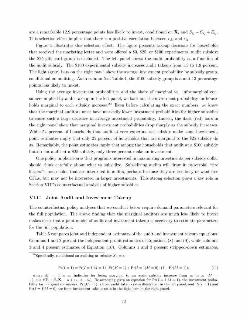
Figure 3 illustrates this selection effect. The figure presents takeup decisions for households
that received the marketing letter and were offered a $0, $25, or $100 experimental audit subsidy;
the $25 gift card group is excluded. The left panel shows the audit probability as a function of
the audit subsidy. The $100 experimental subsidy increases audit takeup from 1.3 to 1.9 percent.
The light (gray) bars on the right panel show the average investment probability by subsidy group,
conditional on auditing. As in column 5 of Table 4, the $100 subsidy group is about 13 percentage
points less likely to invest.
Using the average investment probabilities and the share of marginal vs. inframarginal con-
sumers implied by audit takeup in the left panel, we back out the investment probability for house-
holds marginal to each subsidy increase.20 Even before calculating the exact numbers, we know
that the marginal auditors must have markedly lower investment probabilities for higher subsidies
to cause such a large decrease in average investment probability. Indeed, the dark (red) bars in
the right panel show that marginal investment probabilities drop sharply as the subsidy increases.
While 54 percent of households that audit at zero experimental subsidy make some investment,
point estimates imply that only 25 percent of households that are marginal to the $25 subsidy do
so. Remarkably, the point estimates imply that among the households that audit at a $100 subsidy
but do not audit at a $25 subsidy, only three percent make an investment.
One policy implication is that programs interested in maximizing investments per subsidy dollar
should think carefully about what to subsidize. Subsidizing audits will draw in proverbial “tire
kickers”: households that are interested in audits, perhaps because they are less busy or want free
CFLs, but may not be interested in larger investments. This strong selection plays a key role in
Section VIII’s counterfactual analysis of higher subsidies.
VI.C Joint Audit and Investment Takeup
The counterfactual policy analyses that we conduct below require demand parameters relevant for
the full population. The above finding that the marginal auditors are much less likely to invest
makes clear that a joint model of audit and investment takeup is necessary to estimate parameters
for the full population.
Table 5 compares joint and independent estimates of the audit and investment takeup equations.
Columns 1 and 2 present the independent probit estimates of Equations (8) and (9), while columns
3 and 4 present estimates of Equation (10). Columns 1 and 3 present stripped-down estimates,
20Specifically, conditional on auditing at subsidy SA = s,
Pr(I = 1) = Pr(I = 1|M = 1) · Pr(M = 1) + Pr(I = 1|M = 0) · (1− Pr(M = 1)), (11)
where M = 1 is an indicator for being marginal to an audit subsidy increase from s0 to s: M =1 (−s < τTi + βAXi + κ+ εAi < −s0). Re-arranging gives an equation for Pr(I = 1|M = 1), the investment proba-bility for marginal consumers. Pr(M = 1) is from audit takeup rates illustrated in the left panel, and Pr(I = 1) andPr(I = 1|M = 0) are from investment takeup rates in the light bars in the right panel.
22

excluding household covariates Xi, while columns 2 and 4 include Xi and replace the constant ξj
with separate indicators for all six investment categories: air sealing, insulation, heating/cooling
systems, windows, pipe and duct sealing and insulation, and programmable thermostats. The top
panel of column 2 is the same as column 1 of Table 3, while the bottom panel of column 1 is the
same as column 1 of Table 4, except that we now present coefficient estimates, not marginal effects.
The experimental audit subsidy SEi, gift card indicator Gi, and letter treatment indicator Ti
are included in the audit takeup equation but excluded from the investment takeup equation, thus
identifying the correlation between εAi and εij .21 The estimated ρ ≈ 0.94 is remarkably high, driven
by the sharp decrease in investment probability at higher subsidy levels illustrated in Figure 3.
Comparing the independent and joint estimates in columns 1 vs. 3 and 2 vs. 4, we see that the
audit takeup parameters are all statistically indistinguishable. The investment takeup parameters,
however, are all statistically different. The starkest difference is that the “constant” terms ηIξj are
much more negative in the joint estimates in column 3 compared to the independent estimates in
column 1. This reflects the positive correlation between εAi and εij . In column 1, the independent
probit estimate of investment takeup identifies the constant ηIξj relevant for the subset of house-
holds that audited. By contrast, the joint estimate in column 3 returns the constant relevant for
the full population. The subsample of audited households have high draws of εAi, and because ρ
is large, they also have high draws of εij . Thus, the constant ηIξj for the audited sample is much
larger (i.e. less negative) than for the full sample of 101,881 households. This underscores that the
households that audited are a self-selected group that is significantly more interested in making
investments.
Dividing the estimated constant term ηIξj by ηI gives ξj , the mean unobserved attribute, in
units of dollars. In column 1, we find that across all recommended investments in the sample of
audited households, the mean unobserved attribute is slightly positive: ξj ≈ 0.0485/0.147 ≈ $329.
This indicates that on average, audited households positively value recommended energy efficiency
investments above their financial net present value, perhaps due to warm glow or the expectation
of a more comfortable weatherized home. This approach is important because it captures and
respects consumers’ preferences, allowing for the possibility that consumers perceive costs and
benefits that the analyst does not observe. These results contrast with the assumption in the
“accounting approach” that the mean unobserved attribute is zero.
Figure 4 presents the estimated ξj from a regression that is identical to the investment takeup
probit in column 1, except that it allows the constant term to vary by investment category. We
calculate standard errors using the Delta method. The close correspondence between takeup rates
(against the right axis) and ξj (against the left axis) emphasizes that takeup rates identify ξj : if
many consumers adopt an investment after being informed about its costs and benefits, we infer
that they must derive more utility from it. Air sealing, insulation, and programmable thermostats
have the most positive ξj , while windows and pipe and duct sealing/insulation have the most
21We could also use the full set of non-price treatment indicators Ti as excluded variables, but they reduce precisionbecause they do not affect takeup.
23

negative.
VII Effects on Energy Use
VII.A Empirical Strategy
The private and social benefits of energy saved are a crucial part of the welfare evaluation. What are
the empirical estimates of energy savings, and how do they compare to the simulation predictions?
Define Yit as natural gas or electricity use (in therms/day or kWh/day) for household i for the
billing period ending in date t. Pit is a pair of post-audit indicators: to distinguish shorter-term
from longer-term effects, we allow different coefficients on Pit for the first six months vs. later.
For the billing period that includes the audit date, we pro-rate Pit on [0, 1] to reflect the share of
days after the audit. Wit is a vector of two weather controls: average heating degrees and average
cooling degrees in the household’s city (Madison or Milwaukee) over the billing period ending in
t, from NOAA (2015). νi is a household-by-calendar month fixed effect, and µm is the set of
month-of-sample indicators for all months m in the sample.22 The estimating equation is
Yit = αPit + ωWit + νi + µm + εit. (12)
Standard errors are robust and clustered by household to allow for arbitrary serial correlation
in εit.
To compare empirical estimates to the simulation predictions, we also fit Equation (12) with
predicted savings as the dependent variable. Denote Eit as the total predicted daily savings (in
therms/day or kWh/day) for all observed investments made by household i as of the billing period
ending in date t. (Eit = 0 before the first investment is made, and thus Eit = 0 before the audit.)
If the investment install date occurs in the middle of the billing period ending in date t, we pro-rate
predicted savings over the billing period.
The simulated savings are for average weather conditions. If the empirically realized weather
conditions differ, this could make the empirical results differ from predictions even if predictions
are unbiased in average weather. We thus weather-adjust the predictions assuming that savings
scale proportionally in degree days.23 The “realization rate” for natural gas or electricity will be
the ratio of the α for actual energy use to the α for predicted savings.
22For example, there is one µ indicator variable that takes value 1 for all bills t where the midpoint of the billingperiod occurs in January 2012, then another µ for all bills where the midpoint occurs in February 2012, etc. Then,there is one fixed effect ν for all bills of household i with midpoint in January of any year, a second fixed effect forall bills of household i with midpoint in February of any year, etc.
23Specifically, we classify investments into four seasonality categories: constant (hot water and lighting), cooling(cooling system improvements), heating (heating system improvements), and cooling or heating (all others, suchas insulation, air sealing, etc.). For cooling (heating) categories, Ew
it = Eit · WitWi
, where Wit is the mean base-65
cooling (heating) degree days for billing period t and Wi is the average cooling (heating) degrees for household i’scity (Madison or Milwaukee) between 2000 and 2011. The equation for Ew
it for the “cooling or heating” seasonalitycategory is identical except that Wit and Wit are the sum of heating plus cooling degrees. Appendix Table A.9presents robustness checks without the weather adjustment.
24
If Pit⊥εit|(Wit, νi, µm), then α is the average causal effect of the audit and ensuing invest-
ments. Even under this assumption, however, there are two reasons to interpret α carefully. First,
households may simultaneously change utilization behaviors, so α would differ from causal effect of
investments under constant utilization. This is important for interpreting the realization rate be-
cause TREAT and other simulation models predict savings under constant utilization. A realization
rate less than 100 percent could thus reflect either a utilization increase, which the simulation mod-
els are explicitly not trying to capture, or systematic modeling bias, which the simulation models
should be trying to avoid. This is also important for interpreting the accounting welfare analy-
sis, because a utilization increase generates an increase in consumer welfare that the accounting
approach does not capture.
Second, households may make unobserved investments, such as purchasing CFLs or appliances
through retailers not affiliated with the programs. This is clearly important for the realization
rate, because the simulation models only predict savings from observed investments, and for the
accounting welfare analysis, because we do not include the costs of investments we do not observe.
We discuss these issues more below.24
VII.B Empirical Results
VII.B.1 Graphical Results
Figure 5 is a standard event time graph, which illustrates effects and allows a visual test for pre-
trends. To make the figure, we estimate Equation (12) replacing Pit with indicators for each two-
month period within an event window extending 18 months before and after the audit. The figure
combines separate estimates for natural gas and electricity, weighting each two-month period’s
coefficients by sample average retail prices and multiplying by 365 to transform units to annualized
retail energy cost savings.
Figure 5 shows that there are no pre-audit trends in energy use. Immediately after the audit,
energy use decreases. By about six months post-audit, energy use has stabilized at almost $100
less than the pre-audit annual average. Relative to a pre-audit average of about $1800 per year,
this represents a five percent reduction.
The light gray lines are the simulation predictions, from using Eit instead of energy use as
the dependent variable in the same regression. Predicted energy use decreases immediately after
the audit as “direct install” measures (primarily CFLs and low-flow showerheads) are put in, then
decreases gradually over the first six months post-audit as consumers make larger investments. By
about six months post-audit, predicted energy use has stabilized at approximately $150 less than
baseline. Appendix D presents separate figures for natural gas and electricity, as well as a series of
other graphical robustness checks.
24Neither of these two problems is solved by a randomized encouragement research design. Such a design crediblyidentifies the causal impact of the encouragement, but households could also change utilization behaviors or makeunobserved investments.
25

VII.B.2 Estimation Results
Table 6 presents formal estimates of Equation (12). Columns 1 and 2 are for natural gas, while
columns 3 and 4 are for electricity. Columns 1 and 3 use the weather-adjusted simulation predictions
Eit as the dependent variable, while columns 2 and 4 use energy use Yit. Since the typical investment
is predicted to last 20 years and the graph shows savings stabilizing only after about six months
after the audit, we focus on the coefficients for ≥ 6 months.
After six months, the simulations predict 0.444 therms/day natural gas savings and 0.408
kWh/day electricity savings. By contrast, the actual savings were 0.128 therms/day and 1.013
kWh/day. Figure 6 summarizes these results. Natural gas savings amount to only 29 percent of
predictions, while electricity savings are 248 percent of predictions. In total, the average household
that had an audit saves $89 per year in retail gas and electricity costs. The total predicted savings
are $153 per year, so the realization rate is 58 percent at retail prices. We have done extensive
additional analysis and robustness checks; interested readers should see Appendix D.
Because the realization rates are so different between natural gas and electricity (29 vs. 248
percent), the relative weight given to the two fuels matters for the overall realization rate. For
example, because electricity has a higher retail markup over acquisition cost than natural gas,
combining the two fuels at acquisition costs increases the weight on natural gas. Valuing energy at
acquisition cost, the average audited household reduces gas and electricity use by $38 per year, and
the realization rate is 41 percent. Adding externalities and valuing energy at social marginal cost,
the average audited household reduces gas and electricity use by $94 per year, and the realization
rate is 52 percent.
What could explain the difference between simulated and empirically-estimated savings? For
natural gas, additional analyses in Appendix Table A.11 show smaller or statistically zero shortfalls
for large and common investments (insulation and new heating/cooling systems) but particularly
large empirical shortfalls for smaller and less common investments. For electricity, the additional
analyses suggest that the excess savings could result from unobserved actions such as appliance
replacement that would not be recorded in the programs’ administrative data. When adjusting
the accounting welfare analysis in Section VIII for empirically-realized savings, we assume that
the excess electricity savings accrue because of the observed investments, which may cause us
to understate total investment costs for the empirically-estimated energy savings. This will bias
against our finding that program costs outweighed benefits.
The simulation models assume constant utilization before vs. after the investment, and one
natural explanation for the natural gas shortfall could be the “rebound effect,” i.e. that consumers
increase utilization in response to a decrease in the cost of energy services. Appendix D presents
two calculations showing that the rebound effect is highly unlikely to explain the full gas shortfall.
First, a utilization elasticity of -0.98 would be required to explain the full shortfall. By contrast,
the most closely-related estimates of energy utilization elasticity are much smaller: -0.06, -0.3,
and -0.22 for washing machines (Davis 2008), home electricity (Dubin and McFadden 1984), and
autos (Gillingham 2014), respectively. Second, a large indoor temperature change of 7.5 degrees
26

Fahrenheit would be required to explain the full shortfall. By contrast, the Fowlie, Greenstone,
and Wolfram (2015b) find no statistically significant post-weatherization temperature change in a
low-income (and thus likely more price elastic) population in Michigan, and they can reject a post-
weatherization temperature change of more than 1.4 degrees Fahrenheit with 90 percent confidence
in a two-sided test. To the extent that utilization is not fully inelastic, the associated increase
in consumer welfare is excluded from the “accounting approach,” biasing those benefit estimates
downward. In theory, the revealed preference analysis does capture this welfare increase as part of
ξij .
A realization rate of less than 100 percent is consistent with previous findings. Fowlie, Green-
stone, and Wolfram (2015b) find a 40 percent realization rate in their Michigan RCT. They similarly
find that the simulation model overestimates natural gas savings and underestimates electricity sav-
ings, but since gas comprises a larger share of savings, the overall realization rate is far less than 100
percent. The TREAT software developers found median household-level realization rates around
60-70 percent in recent New York study (PSD 2015b), also finding that their model understated
electricity savings and overstated gas savings. DOE’s analysis of realization rates at other Better
Buildings Neighborhood Program sites were 47 percent and 59 percent, respectively, for natural
gas and electricity (DOE 2015c).25
VIII Welfare Analysis
In this section, we present welfare analyses using the “accounting” and “revealed preference” ap-
proaches. First, we detail assumptions for environmental externalities and market failure parame-
ters φij , γAi, and γij .
Both the accounting and revealed preference approaches require estimates of environmental
externalities per unit of energy use, for each of the three fuels in our data: natural gas, electricity,
and fuel oil. We calculate externality reductions in real 2013 dollars using natural gas and heating
oil emission factors (i.e. pollution emissions per unit of energy use) from the AP-42 database (EPA
1995) and electricity emission factors from Holland, Mansur, Muller, and Yates (2015). For each
fuel, we then multiply those emission factors by pollutant-specific marginal damages, also from
Holland, Mansur, Muller, and Yates (2015). Key assumptions for marginal damages are a $39
social cost of carbon, based on estimates from the Interagency Working Group on the Social Cost
of Carbon (2013), a three percent life-cycle leakage rate from natural gas systems from Howarth et
al. (2012) and Abrahams et al. (2015), a $6 million value of a statistical life, and a fine particulate
dose response function from Pope et al. (2002).
The revealed preference approach requires estimates of present discounted value of the uninter-
nalized externality, denoted φij in our model.26 (If environmental externalities are already priced
25Additionally, an early study by the American Council for an Energy Efficient Economy (Nadel and Keating 1991)reviewed 11 prior studies with a mean realization rate of 48 percent. Blasnik (2010) discusses studies from the 1990swith realization rates between 50 and 70 percent.
26Formally, φij is the sum over fuels f ∈ {natural gas, electricity, fuel oil} of the PDV of an investment’s energy
27

into retail marginal energy costs, then they do not distort investment decisions.) As Davis and
Muehlegger (2010) point out, most utilities mark up retail marginal prices above marginal acquisi-
tion cost in order to cover fixed costs such as meter reading and overhead, and this markup partially
offsets the environmental externalities.27 Section IV presented assumptions for energy acquisition
costs, as well as discount rates and investment lifetimes. In our sample, retail marginal prices
exceed acquisition costs by 50 percent and 297 percent for natural gas and electricity, respectively.
Thus, while the mean recommended investment in our sample reduces environmental externalities
by a present discounted value of $598, the mean φij is only $261.
The revealed preference approach also requires estimates of γAi and γij . Our RCT found statis-
tically and economically zero treatment effects of variations designed to identify six informational
and behavioral barriers to audit takeup. In our base case estimates, we therefore assume γAi = 0.
In the context of the Wisconsin programs, most of the investment takeup market failures γij that
have been discussed in the energy efficiency literature are not relevant. The home energy audits and
written audit reports provide clear information about the costs and benefits of possible investments.
There is no credit constraint, as consumers have full financing available. Credit availability also
reduces the potential role of present bias: allowing consumers to borrow means that investment
does not require a reduction in current consumption. Our sample includes only owner-occupied
homes, so there is no landlord-tenant distortion discussed by Davis (2012), Gillingham, Harding,
and Rapson (2012), and Myers (2015). In Table 4, we found no evidence that investment takeup
is affected by asymmetric information problems that might prevent investments’ full benefits from
being capitalized into home re-sale prices. In our base case estimates, we therefore assume that
γij = 0: other than uninternalized externalities, no market failures affect investment takeup. Due to
the inherent uncertainty in these parameters, we will also present welfare estimates under alternative
assumptions for γAi and γij .
VIII.A Welfare Effects Using the “Accounting Approach”
Table 7 presents welfare effects using the “accounting approach.” Costs comprise audit and in-
vestment costs, while benefits comprise energy savings (at acquisition cost) plus environmental
externality reduction.28 We assume that the unsubsidized audit cost is cA = $400, based on typical
market prices. Column 1 uses the simulation predictions to calculate energy and externality reduc-
savings times the retail price distortion:
φij =∑f
T∑t=1
δt · Energy Savedij,f · (Social Marginal Costf −Retail Marginal Pricef ),
where δ is the discount factor, t indexes time, T is the investment lifetime, and Social Marginal Cost is the per-unitacquisition cost plus the per-unit environmental externality.
27A more economically efficient pricing structure would be to pass through fixed costs as fixed monthly charges.Regardless of whether this rate structure is desirable on equity grounds (see Borenstein and Davis (2012)), it stillgenerates a price distortion.
28To be clear, this is the full environmental externality reduction, not the uninternalized externality reduction φ.Environmental externality reduction plus energy savings (at acquisition cost) also equals uninternalized externalityreduction plus energy savings (at retail price).
28

tions. Column 2 multiplies the simulation predictions by realization rates of 2.48 for electricity and
0.29 for natural gas and heating oil, on the basis of Table 6 and Figure 6.29
Under the assumptions of the accounting approach, the programs reduces welfare. Using the
simulation predictions, the Wisconsin programs have a benefit/cost ratio of 0.92 at five percent
discount rates, with an internal rates of return of 4.0 percent. After adjusting for the empirical
shortfall, the benefit/cost ratio is 0.43 and the IRR is negative 4.1 percent.
Is it possible that the two programs that we evaluated happened to have particularly low
returns? In Appendix E, we analyze data from all 37 Better Buildings Neighborhood Programs
nationwide that reported data to the U.S. Department of Energy (DOE). While we were unable
to run experiments or gather recommended investment data from these other sites to carry out
the full revealed preference analysis, we can replicate this accounting evaluation. The national
programs performed worse than the Wisconsin programs. Using the simulation predictions, the
national programs have a benefit/cost ratio of 0.75 at five percent discount rates, with an IRR of
1.5 percent. After adjusting with the DOE’s estimate of the empirical shortfall, the benefit/cost
ratio is 0.38 and the IRR is negative 5.2 percent. By these metrics, society would have been much
better off without these programs.
The results of the accounting approach depend heavily on energy price and externality assump-
tions. Instead of using recent energy prices, one alternative would be to use forecasts over the
investment lifetimes. The U.S. Energy Information Administration (2015) Annual Energy Out-
look predicts that the benchmark Henry Hub natural gas price will average $1.01 higher in real
terms over 2013-2032 than it was over 2011-2014. When passed through to citygate prices, this
would increase acquisition costs (and thus the value of natural gas savings) by 19 percent, slightly
increasing net benefits. We could also proxy for the social marginal cost of electricity using the
cost of a new combined cycle natural gas plant. Using the Annual Energy Outlook levelized cost
estimates from EIA (2015) and our same per-unit externality damage assumptions, we calculate an
electricity social marginal cost of $0.106 per kilowatt-hour, which is 16 percent lower than our main
assumptions. This is lower because while the levelized production cost is higher than 2011-2014
market prices, this is more than offset by the natural gas plant’s relatively low local air pollution
emissions. Using this lower electricity cost would slightly reduce net benefits. Very large changes
to the energy price or externality assumptions would be required to make the programs welfare
enhancing in Table 7: for empirically-adjusted benefits to exceed costs, energy acquisition costs
would need to be 4.2 times larger, all externality damages would need to be 3.3 times larger, or the
social cost of carbon would need to be $239 per ton.
29The vast majority of heating oil savings are from oil-to-gas heating system conversions. Although we do not haveempirical estimates of the realization rates for heating oil, we need to adjust heating oil savings by the natural gasadjustment factor to avoid predicting artificial decreases in total energy use.
29

VIII.B Welfare Effects Using the “Revealed Preference Approach”
VIII.B.1 Simulation Procedure
We now evaluate the welfare impacts of a subsidy change from s0 to s1 using the “revealed preference
approach.” We first show how to determine the welfare effect conditional on one draw of each εAi and
εij , and we then simulate draws over the joint distribution of εAi and εij . In our base case estimates,
we use the simulation predictions of energy savings, which gives an upper bound on welfare effects
both because the empirically-estimated externality reductions are lower and because consumers may
have made investment decisions with the apparently incorrect belief that the simulation predictions
were unbiased.
We must first define several terms. We denote household i’s vector of εAi and εij draws as εi,
and we denote the vector of all households’ εAi and εij draws as ε. We denote the vector of program
subsidies as sp. We use “hats” to signify that a variable depends on empirical estimates, which we
take from the joint estimates in column 4 of Table 5. For example, λi(s; εi) =∑
j∈Ji Iij(s; εij) ·(Vij(s) + εij).
30
The empirical analogue to the utility function in Equation (1) is
Ui(s; ε) = yi − E0i − T (s; ε) + Ai(s; εi) ·
{ (VAi + εAi
)+(λi(s; εi)− λi(sp; εi)
)−γAi −
∑j∈Ji Iij(s; εij) · γij
}. (13)
To understand the terms inside the brackets in Equation (13), recall that VAi + εAi is the
empirical analogue to sAi − cA + ξAi + λi + γAi, the perceived utility from the audit and potential
investments. The λi in our empirical estimate of VAi is λi(sp; εi), corresponding to existing program
subsidies sp. Therefore, to simulate Ui for a counterfactual subsidy s, we subtract λi(sp; εi) and
add λi(s; εi). If we did not do this, utility would be unaffected by a change in investment subsidies.
The final two terms account for possible differences between observed takeup and true utility from
Equation (1). We subtract γAi if consumer i audited, to account for misperceived audit benefits, and
we subtract γij if consumer i made investment j, to account for misperceived investment benefits.
In our base case, where we assume γAi = γij , Equation (13) is a standard estimate of consumer
surplus based on observed market decisions.
Define W (s; ε) as the empirical analogue to social welfare from Equation (5) conditional on a
draw of ε. The empirical analogue to the welfare change in Equation (6) is
∆W =
∫W (s1; ε)− W (s0; ε) dΦ2(εAi, εij , ρ). (14)
30When fitting Ai and VAi, we make two modifications. First, the latent utility from auditing did not include aterm for the (non-experimental) program audit subsidy offer, as this would have been collinear in the estimation.To simulate counterfactuals at different subsidy levels, we re-write the audit takeup intercept as a function of theprogram audit subsidy sAi offered to household i: κA = κAi + sAi. Second, to reflect conditions in the absence of ourRCT, we set SEi = Gi = Ti = 0.
30

We simulate the integral over 250 draws of ε and present the mean of results across draws.
Because the sample is so large, results are very similar even with many fewer draws.31
We present two tables of results. First, we evaluate the program subsidies and alternative
policies under our base case assumptions for φij , γAi, and γij . Second, we evaluate the program
subsidies under alternative assumptions. The broad array of counterfactuals and assumptions
illustrates the applicability of our approach to a broad class of settings.
VIII.B.2 Results: Program Subsidies and Alternative Policies Under Base Case As-
sumptions
Table 8 reports the simulated effects of alternative residential energy efficiency programs with
different audit and investment subsidies. Panel A details the specific program subsidy assumptions,
Panel B reports the impacts on households and uninternalized externalities, and Panel C presents
welfare impacts.
Column 1 reports the baseline case with audit and investment subsidies set to zero. This coun-
terfactual indicates that the market for home energy audits and retrofits would almost entirely
disappear in the absence of government intervention. For example, the results suggest that over
the sample period, only 0.008 percent of households would have an audit, and only 0.005 percent of
possible energy efficiency investments would be adopted. Across all 101,881 households in the sam-
ple, the mean investment expenditures are $0.21, and the mean value of uninternalized externality
benefits φij from adopted investments is $0.02. This finding, like the others in the table, requires
extrapolation along the audit and investment demand curves, which assume a particular functional
form for the joint distribution of εAi and εij . Notwithstanding, the qualitative implication seems
clear.
Column 2a presents the revealed preference welfare evaluation of the Wisconsin programs at the
subsidy levels employed in these programs. Panel A restates that the audit subsidies were $200 and
$300 in Madison and Milwaukee, respectively, and that we use the linearized investment subsidy
of $5000Eij
E0i, i.e. 5,000 times the predicted share of savings in household energy use. The mean
investment subsidy offer is 24 percent of investment cost. The estimates in Panel B suggest that
the program subsidies effectively create this market, increasing audit and investment takeup rates
to 1.17 and 0.65 percent, respectively. The costs of creating the market are also evident: $14.44
per sample household to fund audit and investment subsidies, or about $1.5 million in total across
all 101,881 sample households. Under these subsidies, the average sample household spends $40.35
on energy efficiency investments, which sums to $4.1 million in the full sample. The investments
are projected to produce around $9.62 of uninternalized externality reductions over their lifetimes
31When simulating ∆W , any household in the sample could be predicted to audit when it receives high simulationdraws of εi, but we do not have characteristics of recommended investments for households that did not audit.For these households, we simulate characteristics of recommended investments with a random draw of the Ji for ahousehold that did audit. We find no evidence against this approach: as shown in Appendix Table A.14, the costs,energy savings, and count of a household’s recommended investments are highly insignificantly correlated with thehousehold’s experimental audit subsidy.
31

per sample household, or about $0.67 per dollar of subsidies.
Panel C presents the simulated social welfare effects of subsidies compared to the zero-subsidy
counterfactual in column 1. The first two rows of Panel C consider the two components of social
welfare. The first row reports the change in consumer utility. Per Equation (13), this depends
on subsidy amounts, the monetary benefits and costs of investments, draws of εAi and εij , and
the resulting takeup decisions and lump-sum taxes to fund the subsidies. In this scenario, the
existing Wisconsin programs reduce consumer utility (ignoring externalities) by $12.22 per sample
household. All scenarios, including the social optimum, involve a decrease in consumer utility
because households are being taxed to induce themselves to make decisions that they would not
otherwise make, thus distorting choices from the perceived private optimum. Of course, these losses
can be offset with social gains from uninternalized externality reduction. The second row of Panel
C shows that relative to the no subsidy counterfactual, the program subsidies induce investments
that reduce uninternalized externalities by an average of $9.61 per sample household.
The social welfare change is the consumer utility change plus the uninternalized externality
reduction. In total, the program subsidies generate a social welfare loss of $2.61 per household, or
about $254,000 in aggregate in our sample. This amounts to a social loss of $0.18 for every $1 in
subsidy. Thus, from the perspective of our model, the program subsidies are worse than having no
subsidies at all.
Great increases in residential energy efficiency investments play an important role in virtually
all climate mitigation plans. Column 2b probes the feasibility of achieving this goal by tripling both
audit and investment subsidies. To be clear, this scenario is relatively extreme. It involves $600
and $900 audit subsidies in Madison and Milwaukee, respectively, so given a market price of $400,
households would receive $200 and $500 to have an audit. The average investment subsidy offer
would be 69 percent of cost. Thus, it is not surprising that this causes 9.94 percent of households
to audit over the sample period, or about nine times more than the program subsidies in column
2a.
However, this increase in audits is not matched by an increase in investments: only about
one percent of possible investments in the sample are adopted, and the average investment across
all households is just shy of $70. This finding of a much smaller investment response is largely
explained by the earlier finding that audit subsidy increases draw in households that are increasingly
negatively selected in their interest in making investments. This alternative policy would cost more
than $140 per household in subsidies and would produce only 30 cents of externality reduction per
subsidy dollar, significantly lower than the program’s actual subsidy. Overall, our model implies
that such a subsidy would reduce welfare by about $39 per sample household, meaning that this
sort of program expansion is not justified by this metric.
Columns 3a and 3b explore a different approach to structuring the investment subsidies. Specif-
ically, column 3a considers investment subsidies set to exactly offset the uninternalized externality
φij , while column 3b considers investment subsidies of 2φij . (To parallel the program subsidies,
we also cap these subsidies at $3500 per investment.) In both columns, there is no audit subsidy.
32

Except for the $3500 cap, the column 3a subsidies are socially optimal in our model if γAi = γij = 0
and energy use is fully price inelastic.
There are three differences between the programs’ investment subsidies and the “socially op-
timal” subsidies in column 3a. First, the program subsidies scale as a share of household energy
use instead of the amount of energy conserved. This causes a distortion by encouraging low-usage
households to make investments that generate less uninternalized externality reduction. Second,
the program subsidies are relatively generous: they cover an average of 24 percent of cost, compared
to 16 percent in column 3a. This induces more energy efficiency investment than would be optimal
under our uninternalized externality assumptions.
Third, the program subsidies scale in energy savings (in physical energy units such as million
British thermal units (mmBtu)) instead of uninternalized externality reductions. For any given
fuel, uninternalized externality reductions scale linearly in energy saved. However, our estimates
of the retail price distortions per physical unit of energy very different across the three fuels: as
shown in Appendix Table A.6, retail price is below social marginal cost by $1.75 and $12.01,
respectively, per mmBtu for natural gas and heating oil, while retail price exceeds social marginal
cost by $3.18 per mmBtu of electricity. Different recommended investments at different homes
save different proportions of the three fuels. Thus, the program subsidies induce investments that
save more electricity and less heating oil compared to subsidies that are precisely targeted to the
uninternalized externality. Put more simply, the subsidies induce investments with high energy
reductions that do not necessarily have high uninternalized externality reductions.
These three factors matter a lot. The subsidies in column 3a generate a social welfare gain of
$21.76 per sample household, or $2.22 million across the full Wisconsin sample. This welfare gain
is accomplished with only $8.59 per household in subsidies, and there is $3.06 in uninternalized
externality benefit per dollar of subsidy. The primary driver of this improved performance is that
the uninternalized social costs of heating oil (primarily from carbon and sulfur emissions) are very
large ($12.01 per mmBtu) compared to those from natural gas and electricity ($1.75 and -$3.18
per mmBtu). When we shift from the program investment subsidies in column 2a to investment
subsidies equal to φij in column 3a, the marginal investments tend to be those that conserve
significant amounts of heating oil. Even in column 3b, with subsidies that are double the “social
optimum” in our model, the welfare effect is positive, although this is naturally less positive than
in 3a because subsidies exceeding φij induce some investments with social costs larger than social
benefits.
Columns 4a and 4b focus on the effects of audit subsidies in isolation. Specifically, they present
results for counterfactual programs with zero investment subsidies and audit subsidies equal to
the actual program amounts (column 4a) and twice the program amounts (column 4b). At both
amounts, audit subsidies reduce social welfare. Subsidizing audits is an inefficient way to reduce
uninternalized externalities compared to simply subsidizing uninternalized externality reduction.
Comparing column 4b to column 4a sharply illustrates the impact of self-selection – that is,
the correlation of εAi and εij . The higher subsidy increases audit takeup by a factor of 13, from
33

0.17 percent to 2.26 percent. However, the investment takeup rate and investment expenditures
increase by only a factor of five. The bottom row of Panel B shows that as a result, this subsidy
increase generates only four cents of externality benefit per subsidy dollar, compared to 15 cents
in column 4a. This underscores a core problem that affects efforts to expand energy efficiency
programs by drawing in households with higher audit subsidies: the households that are marginal
to these subsidies are more likely to be “tire-kickers” who are not very interested in making efficiency
investments.
These simulations have limitations. For example, the joint normal functional form assumption
determines how demand responds to counterfactual subsidies, so we must be especially cautious
in interpreting these out-of-sample predictions. Additionally, the investment takeup elasticity is
estimated from non-experimental data and is lower than our ex ante expectations. Furthermore,
there is considerable uncertainty in the market failure parameters γAi, γij , and φij , which we explore
in the next section.
Even noting these limitations, two main qualitative conclusions are likely to be robust. First,
it is important to calibrate energy efficiency program subsidies to the market failures that might
justify them, and failing to do so can leave surprising amounts of money on the table. This message
may be even more important outside of the Wisconsin programs: many other programs across the
country offer investment subsidies that scale as a percentage of investment costs, thus encouraging
high-cost investments with no regard for either energy savings or environmental benefits. Second,
subsidizing audits can be an ineffective way to reduce externalities, both because audits don’t
directly generate externality reduction and because audit subsidy increases draw in consumers who
are less and less interested to invest.
VIII.B.3 Results: Program Subsidies Under Alternative Assumptions
Table 9 presents welfare evaluations of the existing program subsidies (i.e. those in column 2a of
Table 8) under alternative assumptions for γAi, γij , and φij . Panel A describes the alternative
assumptions for each scenario, including the assumed γAi and the average assumed γij and φij
across all recommended investments. Panel B presents the welfare results, paralleling the bottom
panel of Table 8.
Column 1 re-prints the base case assumptions, giving the same welfare results as column 2a of
Table 8. Column 2 considers a scenario in which energy efficiency improvements are not capitalized
into home resale prices due to asymmetric information problems between home sellers and buyers.
While we do not formally model the details of this asymmetric information problem, we can capture
its implications: existing homeowners that improve energy efficiency effectively impose positive
externalities on future home buyers who receive a more energy efficient home without paying a
higher price. As a benchmark, we add a positive externality of 40 percent of the present discounted
value of empirically-adjusted retail energy cost savings.32 Under this assumption, the program
32This is roughly consistent with a homeowner who sells after 10 years and capitalizes none of the investment inthe sale price, giving the buyer another ten years of a 20-year investment lifetime at a five percent annual discount
34

subsidies generate 41 cents of net social welfare gains for each subsidy dollar spent.
Column 3 presents results after doubling the social cost of carbon, using $78 instead of $39.
The average environmental externality increases by less than a factor of two, because externalities
include local air pollutant emissions as well as carbon, but the average uninternalized externality
(i.e. environmental externality net of the retail energy price markup) more than doubles. The
program subsidies now significantly increase welfare, generating 67 cents in net social welfare gains
per subsidy dollar.
Columns 4-6 take into account the results in Section VII that the simulation predictions over-
state natural gas savings and understate electricity savings. In column 4, we empirically adjust only
the uninternalized externality φij . This is not the same as simply reducing all φij by the 58 percent
realization rate calculated earlier. Instead, the empirically-adjusted average φij of recommended
investments happens to be almost exactly zero, meaning that on average, the energy conserved by
recommended investments is priced very close to social marginal cost. This happens because we
calculate that the retail marginal price is above social marginal cost for electricity, while it is be-
low social marginal cost for natural gas. The empirical adjustment weights electricity substantially
more, and gas substantially less, so this re-weighting reduces the average uninternalized externality.
Naturally, the substantial reduction in uninternalized externality benefits substantially worsens the
program’s estimated welfare effects.
Column 5 takes the next step and assumes that consumers took the audit report’s energy
savings predictions at face value, whereas only the empirically-adjusted savings were realized. This
misperception implies deadweight loss, because consumers made investments that they would not
have made if they knew that the true savings were lower. We accommodate this in the model
by calculating the “actual savings” for investment ij (by multiplying the simulation predictions
of savings on the audit report by the fuel-specific realization rates from Table 6), then setting
γij equal to the simulation predictions minus the “actual savings.” In this scenario, the program
subsidies generate a large social welfare loss of $1.92 per subsidy dollar, or $2.8 million for the full
sample. This starkly highlights how important it is for energy efficiency programs to accurately
inform consumers about how much energy they can expect to save.
Column 6 repeats column 5, except after doubling the social cost of carbon. This somewhat
improves the welfare results, although the improvement is attenuated by the fact that the carbon
savings are attenuated by the empirically estimated realization rates.
In column 7, we leave aside our own assumptions for γAi, γij , and φij and assume that the pro-
gram subsidies were optimally calibrated: that is, that γAi is $200 ($300) in Madison (Milwaukee),
and φij = $5000Eij
Ei0, truncated at $3500. Under these assumptions, the existing program subsidies
would be socially optimal, and they would achieve the first best in our model if home energy use
were fully price inelastic. The welfare gains amount to $2.17 per sample household, or $220,000 for
the full sample.
rate.
35
VIII.C Discussion
Both the “accounting” and “revealed preference” welfare approaches ignore important additional
issues. First, the “revealed preference” model abstracts away from dynamic considerations. At
least in theory, consumers might delay such investments due to uncertainty about future energy
prices (Metcalf and Rosenthal 1995), although we have seen no empirical or anecdotal evidence
that this actually happens. Furthermore, consumers’ ξAi and ξij could vary over time, for example
as they get a raise, move into a new house, or because their interest in home improvements varies
with the age of their house or their personal circumstances. We think of our takeup estimates as
reflecting the takeup that would be expected over a period like our sample period, and we could
expect additional takeup over a longer period as households receive new draws of ξAi and ξij .
Second, the calculations exclude administrative and marketing costs. In total, the Wisconsin
Better Buildings programs facilitated $25.4 million in retrofit costs and also incurred $528,000 in
marketing and outreach and $11.2 million in other program expenses (DOE 2015b). Applying
this 0.46 ratio of overhead/retrofit costs to the investment costs in the experimental sample gives
overhead costs of $2.1 million. This reduces the benefit/cost ratios in Table 7 to 0.65 and 0.30 with
the simulation predictions and empirical adjustment, respectively. $2.1 million is just slightly less
than the welfare gains from the “socially-optimal” subsidies in Column 3a of Table 8.
Third, part of the goal of the Better Buildings programs was to make investments that would
support an economically sustainable home retrofit market. On the basis of their budget records,
WECC staff tell us that more than $7.9 million of WECC’s $20 million EECBG grant was spent
in ways that continued to support local retrofit markets after the grant ended, including a loan
loss reserve, program design efforts, technical training and mentoring for contractors, and funding
for cities to continue parts of the programs (Curtis 2017). This does not affect the interpretation
of Tables 7 and 8, as those include only direct audit and investment costs, but it means that
the overhead costs discussed in the above paragraph have additional benefits that we have not
quantified.
Fourth, the Better Buildings programs were funded with economic stimulus dollars, and job
creation was an important motivation.33 Our analysis is designed to ask whether these programs
would be welfare enhancing in the absence of a macroeconomic stimulus benefit.
IX Conclusion
This paper lays out a framework to evaluate the welfare impacts of residential energy efficiency
programs in the presence of imperfect information, behavioral biases, and externalities, and im-
plements the framework with the help of a 100,000-household randomized field experiment. This
exercise demonstrates that standard revealed preference analysis can be used to evaluate residential
energy efficiency programs and that the results can be used to assess a wide range of policies.
33DOE (2015c) finds that BBNP created or retained net 10,191 full-time-equivalent jobs, or about one job for every$44,000 in federal outlays.
36
The empirical results are remarkable in that they run counter to many aspects of the conven-
tional wisdom about energy efficiency programs. First, the data provide no statistically or eco-
nomically significant evidence of any of the six potential informational and behavioral failures that
were tested. Second, consumer decisions imply large unobserved benefits and costs that conven-
tional accounting-style evaluations do not measure. Third, there is evidence of strong self-selection
in these programs, such that it is less socially beneficial to increase audit subsidies because the
marginal participants are less likely to make externality-reducing investments. Fourth, the esti-
mated energy savings from energy efficiency investments are only 58 percent of predicted savings.
Fifth, the programs reduced welfare. In the accounting-style evaluation, the programs have an in-
ternal rate of return of negative 4.1 percent. In our revealed preference model, the programs reduce
welfare by $0.18 per subsidy dollar. The welfare results demonstrate the significant implications of
even subtle-seeming policy design issues.
While these results may not be encouraging for the program structure we evaluated, the counter-
factual simulations suggest that if Pigouvian taxes or other more direct approaches are not feasible,
there are significant opportunities for energy efficiency programs to increase welfare. Specifically,
we find that a program with perfectly-calibrated subsidies could increase welfare by $2.53 per sub-
sidy dollar. It is apparent that residential energy efficiency programs have significant potential,
but reaching this potential requires restructuring policies to better target the market failures that
motivate them.
References
[1] Abrahams, Leslie S., Constantine Samaras, W. Michael Griffin, and H. Scott Matthews. 2015. “LifeCycle Greenhouse Gas Emissions From U.S. Liquefied Natural Gas Exports: Implications for EndUses.” Environmental Science and Technology 49: 3237-3245.
[2] Allcott, Hunt (2013). “The Welfare Effects of Misperceived Product Costs: Data and Calibrations fromthe Automobile Market.” American Economic Journal: Economic Policy , Vol. 5, No. 3 (August), pages30-66.
[3] Allcott, Hunt, and Michael Greenstone (2012). “Is There an Energy Efficiency Gap?” Journal of Eco-nomic Perspectives, Vol. 26, No. 1 (Winter), pages 3-28.
[4] Allcott, Hunt, and Richard Sweeney (2016). “The Role of Sales Agents in Information Disclosure:Evidence from a Field Experiment.” Management Science, forthcoming.
[5] Allcott, Hunt, and Dmitry Taubinsky (2015). “Evaluating Behaviorally-Motivated Policy: ExperimentalEvidence from the Lightbulb Market.” American Economic Review , Vol. 105, No. 8 (August), pages2501-2538.
[6] Alliance to Save Energy (2013). “Energy Efficiency and the President’s Climate Action Plan.” Avail-able from http://www.ase.org/resources/energy-efficiency-and-presidents-climate-action-plan. AccessedSeptember 13, 2016.
[7] Altonji, Joseph (1993). “The Demand for and Return to Education When Education Outcomes AreUncertain.” Journal of Labor Economics, Vol. 11, No. 1 (August), pages 48-83.
37

[8] American Council for an Energy Efficient Economy (2015). “Section 111(d) of the Clean Air Act.”Available from http://aceee.org/topics/section-111d-clean-air-act. Accessed June 8, 2015.
[9] Attari, Shahzeen, Michael DeKay, Cliff Davidson, and Wandi Bruine de Bruin (2010). “Public Percep-tions of Energy Consumption and Savings.” Proceedings of the National Academy of Sciences, Vol. 107,pages 16054-16059.
[10] Berry, Linda (1984). “The Role of Financial Incentives in Utility-Sponsored Residential ConservationPrograms: A Review of Customer Surveys.” Evaluation and Program Planning , Vol. 7, No. 2, pages131-141.
[11] Bertrand, Marianne, Dean Karlan, Sendhil Mullainathan, Eldar Shafir, and Jonathan Zinman (2010).“What’s Advertising Content Worth? Evidence from a Consumer Credit Marketing Field Experiment.”Quarterly Journal of Economics, Vol. 125, No. 1 (February), pages 263-306.
[12] Bhargava, Saurabh, and Dayanand Manoli (2015). “Psychological Frictions and the Incomplete Take-Up of Social Benefits: Evidence from an IRS Field Experiment.” American Economic Review , Vol. 105,No. 11 (November), pages 3489-3529.
[13] Billingsley, Megan, Ian Hoffman, Elizabeth Stuart, Steven Schiller, Charles Goldman, and KristinaLaCommare (2014). “The Program Administrator Cost of Saved Energy for Utility Customer-Funded Energy Efficiency Programs.” Lawrence Berkeley National Laboratory Report No. 6595E.https://emp.lbl.gov/sites/all/files/lbnl-6595e.pdf
[14] Blasnik, Michael (2010). “Energy Models vs. Reality.” Presentation, Southface Lecture Series (January).
[15] Bloom, Nicholas, Benn Eifert, Aprajit Mahajan, David McKenzie, and John Roberts (2013). “DoesManagement Matter? Evidence from India.” Quarterly Journal of Economics, Vol. 128, No. 1 (Febru-ary), pages 1-51.
[16] Borenstein, Severin, and Lucas Davis (2012). “The Equity and Efficiency of Two-Part Tariffs in U.S.Natural Gas Markets.” Journal of Law and Economics, Vol. 55, No. 1, pages 75-128.
[17] Bronnenberg, Bart, Jean-Pierre Dube, Matthew Gentzkow, and Jesse Shapiro (2015). “Do PharmacistsBuy Bayer? Sophisticated Shoppers and the Brand Premium.” Quarterly Journal of Economics, Vol.130, No. 4 (November), pages 1669-1726.
[18] Bruhn, Miriam, and David McKenzie (2009). “In Pursuit of Balance: Randomization in Practice inDevelopment Field Experiments.” American Economic Journal: Applied Economics, Vol. 1, No. 4(October), pages 200-232.
[19] Bryan, Gharad, Shyamal Chowdhury, and Ahmed Mushfiq Mobarak (2014). “Underinvestment in aProfitable Technology: The Case of Seasonal Migration in Bangladesh.” Econometrica, Vol. 82, No. 5(September), pages 1671-1748.
[20] Camilleri, Adrian R., and Richard P. Larrick (2014). “Metric and Scale Design as Choice ArchitectureTools.” Journal of Public Policy & Marketing , Vol. 33, No. 1 (Spring), pages 108-125.
[21] CEE (Consortium for Energy Efficiency) (2013, 2015). “State of the Efficiency Program Industry.”Boston MA: Consortium for Energy Efficiency. Available from http://www.cee1.org/annual-industry-reports. Accessed May 20, 2015.
[22] Chamberlain, Gary (1980). “Analysis of Covariance with Qualitative Data.” Review of Economic Stud-ies, Vol. 47, pages 225-238.
[23] Chetty, Raj, Adam Looney, and Kory Kroft (2009). “Salience and Taxation: Theory and Evidence.”American Economic Review , Vol. 99, No. 4 (September), pages 1145-1177.
38

[24] Coffman, Lucas, Clayton Featherstone, and Judd Kessler (2016). “Can Social Information Affect WhatJob You Choose and Keep?” American Economic Journal: Applied Economics, forthcoming.
[25] Curtis, Monica (2017). Personal communication. Janary 13th.
[26] Davis, Lucas (2012). “Evaluating the Slow Adoption of Energy Efficient Investments: Are RentersLess Likely to Have Energy-Efficient Appliances?” in The Design and Implementation of U.S. ClimatePolicy, Don Fullerton and Catherine Wolfram, Eds. Chicago, IL: University of Chicago Press.
[27] Davis, Lucas, and Erich Muehlegger (2010). “Do Americans Consume Too Little Natural Gas? AnEmpirical Test of Marginal Cost Pricing.” RAND Journal of Economics, Vol. 41, No. 4, pages 791-810.
[28] Davis, Lucas, and Gilbert Metcalf (2016). “Does Better Information Lead to Better Choices? Evidencefrom Energy-Efficiency Labels.” Journal of the Association of Environmental and Resource Economists,Vol. 3, No. 3 (September), pages 589-625.
[29] DOE (U.S. Department of Energy) (2014). http://energy.gov/eere/wipo/energy-efficiency-and-conservation-block-grant-program. Accessed May 14, 2014.
[30] DOE (U.S. Department of Energy) (2015a). “Better Buildings Neighborhood Program: History.”http://energy.gov/eere/better-buildings-neighborhood-program/history. Accessed June 8, 2015.
[31] DOE (U.S. Department of Energy) (2015b). “Wisconsin Data Dashboard.”http://energy.gov/eere/better-buildings-neighborhood-program/downloads/wisconsin-data-dashboard.Accessed June 13, 2015.
[32] DOE (U.S. Department of Energy) (2015c). “Evaluation of the Better Buildings Neighborhood Pro-gram.” http://www1.eere.energy.gov/analysis/pdfs/bbnp volume 1 final evaluation 072215.pdf. Ac-cessed August 18, 2015.
[33] Dubin, Jeffrey, and Daniel McFadden (1984). “An Econometric Analysis of Residential Electric Appli-ance Holdings and Consumption.” Econometrica, Vol. 52, No. 2 (March), pages 345-362.
[34] Duflo, Esther, Michael Kremer, and Jonathan Robinson (2011). “Nudging Farmers to Use Fertilizer:Theory and Experimental Evidence from Kenya.” American Economic Review , Vol. 101, No. 6, pages2350-2390.
[35] Dupas, Pascaline (2013). “Short-Run Subsidies and Long-Run Adoption of New Health Products: Ev-idence from a Field Experiment.” Econometrica, Vol. 82, No. 1 (January), pages 197-228.
[36] Dupas, Pascaline, and Jonathan Robinson (2013). “Why Don’t the Poor Save More? Evidence fromHealth Savings Experiments.” American Economic Review , Vol. 103, No. 4 (June), pages 1138-1171.
[37] EIA (U.S. Energy Information Administration) (2015). “Annual Energy Outlook.” Available fromhttp://www.eia.gov/forecasts/aeo/. Accessed September 3, 2015.
[38] EPA (U.S. Environmental Protection Agency) (1995). “AP 42, Ffth Edition: Compilation of Air Pol-lutant Emission Factors, Volume 1: Stationary Point and Area Sources. Chapter 1: External Combus-tion Sources.” Available from http://www.epa.gov/ttn/chief/ap42/ch01/index.html. Accessed June 12,2015.
[39] Foster, Andrew, and Mark Rosenzweig (2010). “Microeconomics of Technology Adoption.” AnnualReview of Economics, Vol. 2, pages 395-424.
[40] Fowlie, Meredith, Michael Greenstone, and Catherine Wolfram (2015a). “Are the Non-Monetary Costsof Energy Efficiency Investments Large? Understanding Low Take-up of a Free Energy EfficiencyProgram.” American Economic Review, Papers and Proceedings, forthcoming.
39

[41] Fowlie, Meredith, Michael Greenstone, and Catherine Wolfram (2015b). “Do Energy Efficiency Invest-ments Deliver? Evidence from the Weatherization Assistance Program.” Working Paper, University ofChicago (June).
[42] Gillingham, Kenneth (2014). “Identifying the Elasticity of Driving: Evidence from a Gasoline PriceShock in California.” Regional Science and Urban Economics, Vol. 47 (July), pages 13-24.
[43] Gillingham, Kenneth, Matthew Harding, and David Rapson (2012). “Split Incentives and HouseholdEnergy Consumption.” The Energy Journal , Vol. 33, No. 2, pages 37-62.
[44] Gillingham, Kenneth, Richard Newell, and Karen Palmer (2009). “Energy Efficiency Economics andPolicy.” Annual Review of Resource Economics, Vol. 1, pages 597-619.
[45] Greenstone, Michael, Elizabeth Kopits, and Ann Wolverton (2013). “Developing a Social Cost of Carbonfor US Regulatory Analysis: A Methodology and Interpretation.” Review of Environmental Economicsand Policy , Vol. 7, No. 1, pages 23-46.
[46] Hanna, Rema, Esther Duflo, and Michael Greenstone (2016). “Up in Smoke: The Influence of House-hold Behavior on the Long-Run Impact of Improved Cooking Stoves.” American Economic Journal:Economic Policy , Vol. 8, No. 1 (February), pages 80-114.
[47] Heckman, James (1979). “Sample Selection Bias as a Specification Error.” Econometrica, Vol. 47, No.1 (January), pages 153-161.
[48] Holland, Stephen, Erin Mansur, Nicholas Muehller, and Andrew Yates (2015). “Measuring the SpatialHeterogeneity in Environmental Externalities from Driving: A Comparison of Gasoline and ElectricVehicles.” NBER Working Paper No. 21291 (June).
[49] Howarth, Robert, Drew Shindell, Renee Santoro, Anthony Ingraffea, Nathan Phillips, andAmy Townsend-Small. (2012). “Methane Emissions from Natural Gas Systems.” Available fromhttp://www.eeb.cornell.edu/howarth/publications/Howarth et al 2012 National Climate Assessment.pdf.Accessed August 15, 2015.
[50] Interagency Working Group on the Social Cost of Carbon (2013). “Techni-cal Support Document - Technical Update of the Social Cost of Carbon forRegulatory Impact Analysis - Under Executive Order 12866.” Available fromhttp://www.whitehouse.gov/sites/default/files/omb/inforeg/social cost of carbon for ria 2013 update.pdf
[51] International Energy Agency (2015). “World Energy Outlook 2015.” Available fromhttp://www.worldenergyoutlook.org/weo2015/. Accessed August 18, 2016.
[52] Jaffe, Adam, and Robert Stavins (1994). “The Energy-Efficiency Gap: What Does it Mean?” EnergyPolicy , Vol. 22, No. 10, pages 804-810.
[53] Kushler, Martin, Seth Nowak, and Patti Witte (2012). “A National Survey of State Policies and Prac-tices for the Evaluation of Ratepayer-Funded Energy Efficiency Programs.” American Council for anEnergy-Efficient Economy Report Number U122 (February).
[54] Mandel, Naomi, and Eric Johnson (2002). “When Web Pages Influence Choice: Effects of Visual Primeson Experts and Novices.” Journal of Consumer Research, Vol. 29, pages 235–245.
[55] Manski, Charles (1988). “Should We Subsdize Enrollment in or Completion of Postsecondary School-ing?” Available from http://files.eric.ed.gov/fulltext/ED315523.pdf.
[56] McKinsey & Co. (2009). “Unlocking Energy Efficiency in the U.S. Economy.” Available fromhttp://www.mckinsey.com/clientservice/electricpowernaturalgas/downloads/US energy efficiency full report.pdf.Accessed June 25, 2014.
40

[57] Metcalf, Gilbert, and Donald Rosenthal (1995). “The “New” View of Investment Decisions and PublicPolicy Analysis: An Application to Green Lights and Cold Refrigerators.” Journal of Policy Analysisand Management, Vol. 14, No. 4 (Autumn), pages 517-531.
[58] Meyer, David, and Roger Schvaneveldt (1971). “Facilitation in Recognizing Pairs of Words: Evidenceof a Dependence Between Retrieval Operations.” Journal of Experimental Psychology , Vol. 90, pages227-234.
[59] Mullainathan, Sendhil, Joshua Schwartzstein, and William Congdon (2012). “A Reduced-Form Ap-proach to Behavioral Public Finance.” Annual Review of Economics, Vol. 4, pages 17.1-17.30.
[60] Myers, Erica (2015). “Asymmetric Information in Residential Rental Markets: Implicationsfor the Energy Efficiency Gap.” Working Paper, UC Berkeley (September). Available fromhttps://ei.haas.berkeley.edu/research/papers/WP246.pdf
[61] Nadel, Steven, and Kenneth Keating (1991). “Engineering Estimates vs. Impact Evaluation Results:How Do They Compare and Why?” Research Report U915, American Council for an Energy-EfficientEconomy. Available from http://www.aceee.org/research-report/u915
[62] National Association of State Energy Officials (2015). “State 111(d) Resource Hub.” Available fromhttp://111d.naseo.org/. Accessed June 8, 2015.
[63] Newell, Richard, and Juha Siikamaki (2013). “Nudging Energy Efficiency Behavior: The Role of Infor-mation Labels.” NBER Working Paper No. 19224 (July).
[64] NOAA (National Oceanic and Atmospheric Administration) (2015). “Climate Data Online.” Availablefrom http://www.ncdc.noaa.gov/cdo-web/search. Accessed June 14, 2015.
[65] Pope, C. Arden, Richard T. Burnett, Michael J. Thun, Eugenia, E. Calle, Daniel Krewski, Kazuhiko Ito,and George D. Thurston (2002). “Lung Cancer, Cardiopulmonary Mortality, and Long-term Exposureto Fine Particulate Air Pollution.” Journal of the American Medical Association, Vol. 287, No. 9 (March6), pages 1132-1141.
[66] Potomac Economics (2012-2015). “State of the Market Report for the MISO Electricity Markets.” Avail-able from https://www.misoenergy.org/MarketsOperations/IndependentMarketMonitor/Pages/IndependentMarketMonitor.aspx.Accessed August 18, 2015.
[67] PSD (Performance Systems Development) (2015a). “HERS BESTEST & DOE APPROVED.” Availablefrom http://psdconsulting.com/software/treat/hers-bestest-doe-approved/. Accessed June 8, 2015.
[68] PSD (Performance Systems Development) (2015b). “NYSERDA Home Performance with Energy StarRealization Rate Attribution Study.” Prepared for New York State Energy Research and DevelopmentAuthority. Ithaca, NY: Performance Systems Development.
[69] Sanstad, Alan, Michael Hanemann, and Maximilian Auffhammer (2006). “End-use Energy Efficiencyin a “Post-Carbon” California Economy: Policy Issues and Research Frontiers.” In Michael Hanemannand Alexander Farrell, Eds., Managing Greenhouse Gas Emissions in California. Berkeley, CA: TheCalifornia Climate Change Center at UC Berkeley.
[70] Skumatz, Lisa (2008). “Non-Energy Benefits Publications / Bibliography for Skumatz / SERA.” Avail-able from http://www.serainc.com/NEBPublicationsforWebSite2008.pdf. Accessed July 9, 2015.
[71] Suri, Tavneet (2011). “Selection and Comparative Advantage in Technology Adoption.” Econometrica,Vol. 79, No. 1, pages 159–209.
[72] Turrentine, Thomas, and Kenneth Kurani (2007). “Car Buyers and Fuel Economy?” Energy Policy ,Vol. 35, pages 1213-1223.
41

[73] Van de Ven, Wynand, and Bernard Van Praag (1981). “The Demand for Deductibles in Private HealthInsurance.” Journal of Econometrics, Vol. 17, pages 229-252.
[74] Yergin, Daniel (1979). Energy Future: The Report of the Energy Project at the Harvard BusinessSchool. New York: Random House.
42

Tables and Figures
Table 1: Overview of Related Energy Efficiency Programs
Panel A: Policy Overview
(1) (2) (3) (4)
Better Buildings Energy Efficiency U.S. and Canada Weatherization
Neighborhood and Conservation Ratepayer-Funded Assistance Program
Program Block Grants Efficiency Programs (per year,
(2010-2013) (total) (year 2013) pre-stimulus)
Number of programs 41 ∼2000 347 ∼400
Public expenditures $508 million $3.2 billion $8.0 billion $250 million
Buildings retrofitted 119,404 86,000 100,000
Value of predicted energy saved $669 million $2.95 billion $453 million
Panel B: Program Evaluation Assumptions
Share of programs
Include non-monetary benefits 30%
Use simulation predictions of savings 97%
of which: Use simulation predictions from other states 70%
Do not evaluate programs retrospectively 81%Notes: “Public expenditures” includes costs of program operation, including administrative costs and subsi-dies, but not any investment costs paid by consumers. Better Buildings Neighborhood Program informationin column 1 is from DOE (2015b,c). Energy Efficiency and Conservation Block Grant information in column2 is from DOE (2014). U.S. and Canada ratepayer-funded program information in column 3 is from CEE(2015), and energy savings are those that accrue in 2013 only. Weatherization Assistance Program informa-tion in column 4 is from DOE (2011,2015) and Eisenberg (2010). Program evaluation assumptions are fromKushler, Nowak, and Witte (2012).
43

Table 2: Summary Statistics
Variable Mean Std.
Dev.
Min. Max.
Panel A: Wisconsin Household Data
(N=101,881 households in experimental population)
House age (years) 67.2 23.0 0 182
Property value ($000s) 156 90.7 0 2816
Building footprint (sq. feet/1000) 1.24 0.43 0 12.1
Madison 0.31 0.46 0 1
Census tract hybrid vehicle share 1.20 1.26 0 8.33
Audited 0.014 0.12 0 1
Invested 0.008 0.09 0 1
Panel B: Wisconsin Simulation Estimates of Monetary Costs and Benefits
Recommended investments (N=6100 at the 1394 households that had audits)
Cost ($) 1493 1472 17.1 43,600
Retail energy cost savings ($/year) 86.1 145 0.01 4359
Invested 0.51 0.50 0 1
Adopted investments (N=3834 at the 1394 households that had audits)
Cost ($) 1206 1208 0.5 14,475
Retail energy cost savings ($/year) 79.9 134 -526 2501
Panel C: Wisconsin Electricity and Natural Gas Usage
N=1212 households (gas); N=1217 households (electricity)
Number of gas bills observed 51.9 14.2 9 88
Average gas use (therms/day) 2.50 0.98 0.20 9.59
Number of electricity bills observed 53.2 14.2 8 88
Average electricity use (kWh/day) 20.6 9.27 4.16 80.6
Notes: Recommended investments in Panel B include only those used for empirical estimates of investmenttakeup, and adopted investments in Panel B include only those used for the “accounting approach” towelfare analysis. Energy bills are observed only if a household had an audit. Energy prices are averages over2011-2014. See Appendix B for more details.
44
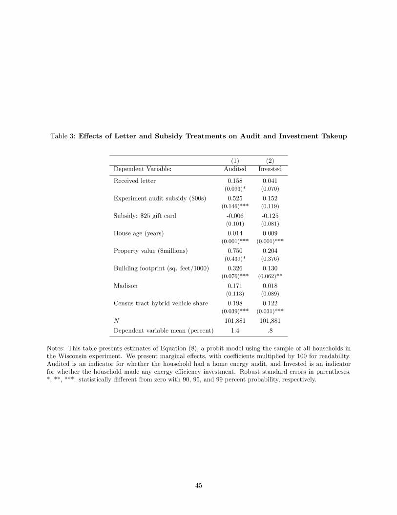
Table 3: Effects of Letter and Subsidy Treatments on Audit and Investment Takeup
(1) (2)Dependent Variable: Audited Invested
Received letter 0.158 0.041(0.093)* (0.070)
Experiment audit subsidy ($00s) 0.525 0.152(0.146)*** (0.119)
Subsidy: $25 gift card -0.006 -0.125(0.101) (0.081)
House age (years) 0.014 0.009(0.001)*** (0.001)***
Property value ($millions) 0.750 0.204(0.439)* (0.376)
Building footprint (sq. feet/1000) 0.326 0.130(0.076)*** (0.062)**
Madison 0.171 0.018(0.113) (0.089)
Census tract hybrid vehicle share 0.198 0.122(0.039)*** (0.031)***
N 101,881 101,881
Dependent variable mean (percent) 1.4 .8
Notes: This table presents estimates of Equation (8), a probit model using the sample of all households inthe Wisconsin experiment. We present marginal effects, with coefficients multiplied by 100 for readability.Audited is an indicator for whether the household had a home energy audit, and Invested is an indicatorfor whether the household made any energy efficiency investment. Robust standard errors in parentheses.*, **, ***: statistically different from zero with 90, 95, and 99 percent probability, respectively.
45
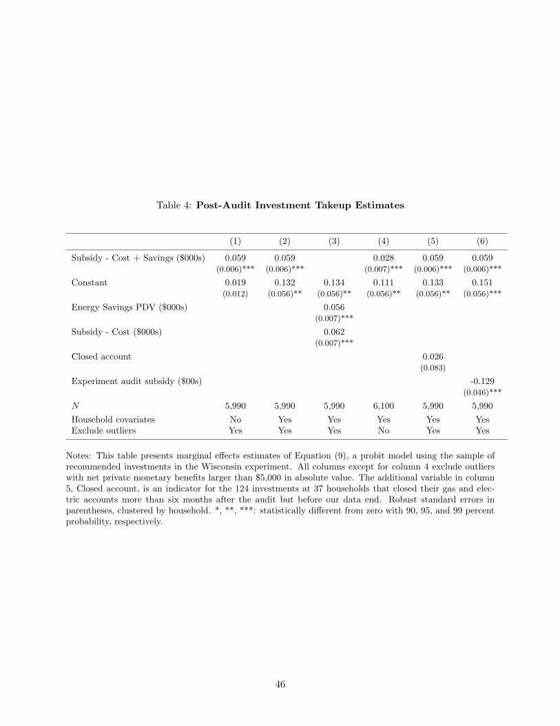
Table 4: Post-Audit Investment Takeup Estimates
(1) (2) (3) (4) (5) (6)
Subsidy - Cost + Savings ($000s) 0.059 0.059 0.028 0.059 0.059(0.006)*** (0.006)*** (0.007)*** (0.006)*** (0.006)***
Constant 0.019 0.132 0.134 0.111 0.133 0.151(0.012) (0.056)** (0.056)** (0.056)** (0.056)** (0.056)***
Energy Savings PDV ($000s) 0.056(0.007)***
Subsidy - Cost ($000s) 0.062(0.007)***
Closed account 0.026(0.083)
Experiment audit subsidy ($00s) -0.129(0.046)***
N 5,990 5,990 5,990 6,100 5,990 5,990
Household covariates No Yes Yes Yes Yes YesExclude outliers Yes Yes Yes No Yes Yes
Notes: This table presents marginal effects estimates of Equation (9), a probit model using the sample ofrecommended investments in the Wisconsin experiment. All columns except for column 4 exclude outlierswith net private monetary benefits larger than $5,000 in absolute value. The additional variable in column5, Closed account, is an indicator for the 124 investments at 37 households that closed their gas and elec-tric accounts more than six months after the audit but before our data end. Robust standard errors inparentheses, clustered by household. *, **, ***: statistically different from zero with 90, 95, and 99 percentprobability, respectively.
46

Table 5: Joint Estimates of Audit and Investment Takeup
(1) (2) (3) (4)
Independent Probits Joint Estimates
Audit Parameters
Received letter 0.0470 0.0482 0.0295 0.0318
(0.0279)* (0.0282)* (0.0253) (0.0254)
Experiment audit subsidy ($00s) 0.156 0.160 0.178 0.182
(0.0438)*** (0.0443)*** (0.0436)*** (0.0447)***
Subsidy: $25 gift card -0.00131 -0.00169 0.0376 0.0372
(0.0304) (0.0307) (0.0280) (0.0281)
Constant -2.260 -2.813 -2.265 -2.833
(0.0236)*** (0.0462)*** (0.0224)*** (0.0459)***
Household covariates No Yes No Yes
Investment Parameters
Subsidy - Cost + Savings ($000s) 0.147 0.119 0.0619 0.0497
(0.0150)*** (0.0173)*** (0.0213)*** (0.0182)***
Constant 0.0485 -2.363
(0.0308) (0.141)***
Investment category indicators No Yes No Yes
Household covariates No Yes No Yes
ρ 0.941 0.944
(0.0599)*** (0.0608)***
Notes: Columns 1 and 2 present the independent probit estimates of Equations (8) and (9), while columns3 and 4 present estimates of Equation (10) using the maximum likelihood estimator of Van de Ven and VanPraag (1981). These are coefficients, not marginal effects. All estimates exclude outlier investments with netprivate monetary benefits larger than $5,000 in absolute value. ρ is the estimated correlation between theerrors in the audit and investment takeup equations. Robust standard errors in parentheses, clustered byhousehold. *, **, ***: statistically different from zero with 90, 95, and 99 percent probability, respectively.
47

Table 6: Post-Audit Energy Use Changes
(1) (2) (3) (4)Natural Gas (therms/day) Electricity (kWh/day)
Simulation Energy Simulation EnergyDependent Variable: Prediction Use Prediction Use
Post audit (<6 months) -0.284 -0.093 -0.296 -0.874(0.026)*** (0.029)*** (0.026)*** (0.238)***
Post audit (≥6 months) -0.444 -0.128 -0.408 -1.013(0.032)*** (0.036)*** (0.036)*** (0.319)***
N 61,845 61,845 63,655 63,654
Notes: This table presents estimates of Equation (12) with daily usage of natural gas and electricity, re-spectively, as the dependent variables. Columns 1 and 3 have the simulation predictions as the dependentvariable, while columns 2 and 4 have energy use as the dependent variable. Mean pre-audit natural gas usageis 2.40 therms/day, and mean pre-audit electricity usage is 21.4 kWh/day. Average marginal natural gasprice is $0.82 per therm, and average marginal electricity price is $0.136 per kWh. All columns control forheating and cooling degrees, household-by-calendar month fixed effects, and month-of-sample fixed effects.Robust standard errors in parentheses, clustered by household. *, **, ***: statistically different from zerowith 90, 95, and 99 percent probability, respectively.
48

Table 7: Welfare Effects: Accounting Approach
(1) (2)
Simulation Empirically
Source of energy savings estimates: Predictions Adjusted
Cost ($millions)
Audit costs (at $400 per audit) 0.56
Investment costs 4.52
Total cost 5.08
Energy Savings ($millions present value at 5% discount rate)
Natural gas 1.92 0.56
Electricity 0.07 0.18
Heating oil 0.61 0.18
Total 2.61 0.92
Externality Reduction ($millions present value at 5% discount rate)
Climate (at $39 per ton CO2) 1.37 0.57
SO2/NOx/PM 0.72 0.68
Total 2.09 1.26
Summary
Benefits - Costs ($millions) -0.39 -2.91
Benefit/Cost ratio 0.92 0.43
Internal rate of return (percent) 4.0 -4.1
Notes: Column 1 uses energy savings projected by simulation models, while column 2 adjusts for empirically-observed savings. Column 2 multiplies electricity and gas/heating oil savings from Column 1 by 2.48 and0.29, respectively, based on the estimates in Table 6. Energy savings are calculated at average wholesaleprices over 2011-2014, and externality reductions are based on a $39 social cost of carbon and a $6 millionvalue of a statistical life; see Appendix B for details.
49

Table 8: Welfare Effects: Revealed Preference Approach
(1) (2a) (2b) (3a) (3b) (4a) (4b)
No Program Externality Audit
Scenario: Subsidy Subsidy Subsidy Only Subsidy Only
Panel A: Program Subsidy Assumptions
Audit subsidy in Madison/Milwaukee $0 $200/300 $600/900 $0 $0 $200/300 $400/600
Investment subsidy multiplier on share energy saved – 5,000 15,000 – – – –
Investment subsidy multiplier on externality reduction – – – 1 2 – –
Panel B: Program Impacts on Households and Externalities
Audit probability 0.008% 1.17% 9.94% 0.27% 0.70% 0.17% 2.26%
Investment probability 0.005% 0.65% 1.03% 0.11% 0.40% 0.03% 0.16%
Subsidy paid per sample household $0 $14.44 $141.95 $8.59 $17.66 $0.59 $13.29
Investment expenditures per sample household $0.21 $40.35 $68.92 $11.69 $31.43 $1.39 $6.42
Uninternalized externality benefit from investments per sample household $0.02 $9.62 $42.94 $26.28 $30.15 $0.09 $0.54
Uninternalized externality benefit per dollar subsidy -- 0.67 0.30 3.06 1.71 0.15 0.04
Incremental uninternalized externality benefit per incremental dollar subsidy 0.67 0.26 0.43 0.04
(relative to previous column)
Panel C: Program Impacts on Welfare (Relative to No Subsidy)
∆Consumer utility (net of tax) per sample household -$12.22 -$82.18 -$4.51 -$10.45 -$0.40 -$10.31
∆Uninternalized externality per sample household $9.61 $42.93 $26.27 $30.14 $0.08 $0.52
∆Welfare per sample household -$2.61 -$39.25 $21.76 $19.69 -$0.33 -$9.79
∆Welfare per dollar subsidy -0.18 -0.28 2.53 1.11 -0.55 -0.74
Incremental ∆welfare per incremental dollar subsidy -0.18 -0.29 -0.23 -0.75
(relative to previous column)Notes: This table reports averages across 250 simulated draws of ε. “Program Subsidy” refers to an investment subsidy that scales in the share ofhousehold energy saved. “Externality Subsidy” refers to an investment subsidy that scales in uninternalized externality reduction. Both subsidies arerestricted to be between $0 and $3,500 per investment. Investment probability divides the number of adopted investments by the total number ofpossible investments that could be made by the 101,881-household sample. “Per sample household” means per household in the 101,881-householdWisconsin sample. Uninternalized externality reductions are discounted at a five percent discount rate using the programs’ assumed investmentlifetimes and simulation predictions of savings, based on a $39 social cost of carbon and a $6 million value of a statistical life; see Appendix B fordetails. In Panel C, consumer utility is from Equation (13), and ∆Welfare is from Equation (14).
50
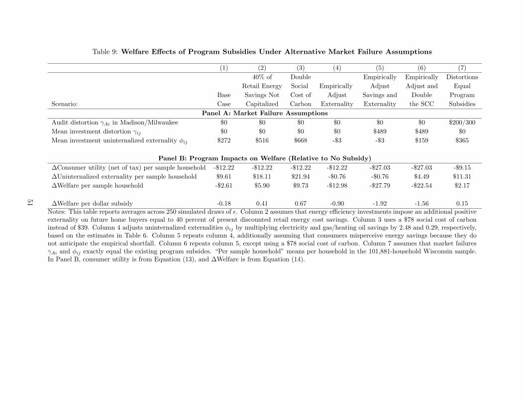
Table 9: Welfare Effects of Program Subsidies Under Alternative Market Failure Assumptions
(1) (2) (3) (4) (5) (6) (7)
40% of Double Empirically Empirically Distortions
Retail Energy Social Empirically Adjust Adjust and Equal
Base Savings Not Cost of Adjust Savings and Double Program
Scenario: Case Capitalized Carbon Externality Externality the SCC Subsidies
Panel A: Market Failure Assumptions
Audit distortion γAi in Madison/Milwaukee $0 $0 $0 $0 $0 $0 $200/300
Mean investment distortion γij $0 $0 $0 $0 $489 $489 $0
Mean investment uninternalized externality φij $272 $516 $668 -$3 -$3 $159 $365
Panel B: Program Impacts on Welfare (Relative to No Subsidy)
∆Consumer utility (net of tax) per sample household -$12.22 -$12.22 -$12.22 -$12.22 -$27.03 -$27.03 -$9.15
∆Uninternalized externality per sample household $9.61 $18.11 $21.94 -$0.76 -$0.76 $4.49 $11.31
∆Welfare per sample household -$2.61 $5.90 $9.73 -$12.98 -$27.79 -$22.54 $2.17
∆Welfare per dollar subsidy -0.18 0.41 0.67 -0.90 -1.92 -1.56 0.15Notes: This table reports averages across 250 simulated draws of ε. Column 2 assumes that energy efficiency investments impose an additional positiveexternality on future home buyers equal to 40 percent of present discounted retail energy cost savings. Column 3 uses a $78 social cost of carboninstead of $39. Column 4 adjusts uninternalized externalities φij by multiplying electricity and gas/heating oil savings by 2.48 and 0.29, respectively,based on the estimates in Table 6. Column 5 repeats column 4, additionally assuming that consumers misperceive energy savings because they donot anticipate the empirical shortfall. Column 6 repeats column 5, except using a $78 social cost of carbon. Column 7 assumes that market failuresγAi and φij exactly equal the existing program subsides. “Per sample household” means per household in the 101,881-household Wisconsin sample.In Panel B, consumer utility is from Equation (13), and ∆Welfare is from Equation (14).
51

Figure 1: Audit Takeup Treatment Effects Scaled by Effect of a $1 Subsidy
Subsidy ($00s)$25 gift card
Audit cue: AssessmentTime: Seven Year
Prime: EnvironmentPrime: Climate
Prime: FinancialFinancing: Incentives
Financing: CreditComparison: Car idlingComparison: Lights on
Comparison: Door openInfo: Combined
Info: EnvironmentInfo: ClimateInfo: Comfort
Info: Financial
-50 0 50 100 150Effect scaled by effect of $1 subsidy ($)
Notes: This figure presents the point estimates and 90 percent confidence intervals for the treatment effectestimates from the Wisconsin audit takeup experiment, scaled by the effect of a $1 subsidy. The estimatingequation is Equation (8), and formal estimates are in Appendix Table A.7.
Figure 2: Net Private Monetary Benefit and Investment Takeup
0.1
.2.3
.4.5
.6.7
Tak
eup
rate
0.0
5.1
Sha
re o
f rec
omm
ende
d in
vest
men
ts
-3000 -2000 -1000 0 1000 2000 3000Net private monetary benefit ($)
Share Takeup rate
Notes: Net private monetary benefit is the present discounted value of retail energy cost savings net ofsubsidized cost, or (Sij − Cij +Eij) in the notation of the model. Energy cost savings are computed at the2011-2014 average retail natural gas and electricity prices in the household’s city (Madison or Milwaukee).Subsidized costs are the upfront cost net of an imputed subsidy of $500 per 10 percentage point projecteddecrease in the household’s pre-audit energy use.
52

Figure 3: Marginal Investment Probabilities by Subsidy Level
0.5
11.
52
Per
cent
of p
opul
atio
n au
ditin
g
$0 subsidy $25 subsidy $100 subsidy
020
4060
Pr(
Inve
st|A
udit)
$0 subsidy $25 subsidy $100 subsidy
Average Marginal
Notes: The left panel presents audit probability for each experimental audit subsidy group. The light (gray)bars on the right panel show the average investment probability by subsidy group, conditional on auditing.The dark (red) bars on the right panel show the investment probability for households marginal to each auditsubsidy increase. Households that were in the letter control group or the $25 gift card group are excludedfrom this figure.
Figure 4: Mean Unobserved Attribute of Recommended Investments
.2.3
.4.5
.6T
akeu
p ra
te
-10
-50
5M
ean
unob
serv
ed a
ttrib
ute
($00
0s)
Airsealing
Insulation New heating/coolingsystem
Newwindows
Pipe/ductsealing/
insulation
Prog.t-stat
Average utility Takeup rate
Notes: Point estimates and 90 percent confidence intervals for the dollar value of the mean unobservedattribute by investment category, or ξj in the notation of the model. This uses estimates in column 1 ofTable 4. Standard errors are calculated using the Delta method.
53

Figure 5: Energy Use in Event Time
-150
-100
-50
050
Ann
ualiz
ed r
etai
l ene
rgy
cost
sav
ings
($)
-18 -12 -6 0 6 12 18Months after audit
Empirical estimate Simulation prediction
Notes: This figure presents energy use in event time relative to the household’s audit. The figure is con-structed by estimating Equation (12) separately for natural gas and electricity, replacing Pit with indicatorsfor each two-month period within an event window extending 18 months before and after the audit. Theexcluded category is the month of the audit and the month before. After estimating separate equations fornatural gas and electricity, we combine coefficients and standard errors for each two-month period, weight-ing fuels by their retail prices and multiplying by 365 to transform units to annualized retail cost savings.Dashed lines are 90 percent confidence intervals. Mean pre-audit retail energy costs are $1804 per year.
Figure 6: Simulation Predictions vs. Empirical Estimates of Post-Audit Energy Savings
050
100
150
Mea
n an
nual
ret
ail e
nerg
y co
st s
avin
gs p
er a
udit
($)
Gas Electricity Combined
Simulation prediction Empirical estimate
Notes: This figure takes the simulated and actual effects on energy use for households ≥6 months post-auditfrom Table 6. The regression coefficients are in therms per day (for gas) and kilowatt-hours per day (forelectricity). They are multiplied by 365 × sample average retail energy prices to give mean annual retailenergy cost savings per audit.
54

Online Appendix Allcott and Greenstone
MEASURING THE WELFARE EFFECTS OF RESIDENTIAL ENERGY EFFICIENCYPROGRAMS
Hunt Allcott and Michael Greenstone
Online Appendix: Not for Publication
1

Online Appendix Allcott and Greenstone
A Example Audit Report
2

Online Appendix Allcott and Greenstone
Figure A.1: Example Audit Report (Page 1)
May 21, 2013 Dear Aaron; You’re on your way to saving energy and money! Your home energy assessment results are in and Milwaukee Energy Efficiency (Me2) is here to help. The enclosed Home Performance with ENERGY STAR® report is your ticket to savings—not to mention a better, more comfortable home. The report tells you how your home performed, including: Facts about your home’s insulation levels, ventilation, and air leakage. What’s really going on—the source of your home’s problems. Personalized and proven solutions to improve your home’s performance.
Me2 provides City of Milwaukee residents with access to more financial offers than ever before. Use available incentives and watch your savings add up: Me2 incentive—Me2 is giving you $750 to $2,000 when you complete all of the recommended measures. Energy assessment reimbursement—Complete recommended air sealing work or $1,000 in other energy
efficiency improvements with a Participating Contractor and you’ll get your $100 energy assessment fee back. Health and Safety Grant—You may qualify for a grant up to $1,000 to fix eligible health and safety issues, including
electrical upgrades of knob and tube wiring and removal of asbestos, vermiculite, or an oil tank. To receive this grant, you must also complete the recommended energy-efficiency improvements.
Special financing—Take advantage of optional energy-efficiency financing through Summit Credit Union. Flexible terms and fixed interest rates lower than average personal loan rates. Visit SummitCreditUnion.com/SummitMe2 or call 800.236.5560 to learn more or to get pre-approved.
Plus, you’ll save on energy bills if you complete the improvements recommended in your report. Next steps You’re so close to having an energy-efficient home. KEEP GOING. Decide which recommended projects you’d like to pursue. Pull out the Participating Contractor List. Ask for estimates, schedule the work, and reap the benefits. Questions? Your Me2 team is here to help. Don’t hesitate to contact me or your energy consultant. We can help answer questions, prioritize projects, and keep things moving forward. Sincerely, Margee Foulke-Evans Me2 Energy Advocate 414-333-6245 [email protected] P.S. Enjoy the perks! Having an energy-efficient home is smart. You’ll save energy and money.
3

Online Appendix Allcott and Greenstone
Figure A.2: Example Audit Report (Page 2)
Reference Home The below diagram is provided for reference as you read your personalized report. It illustrates common sources of home energy-efficiency issues and associated terminology.
4

Online Appendix Allcott and Greenstone
Figure A.3: Example Audit Report (Page 3)
Hom How
RequPROPOImprov Attic Kn
Vaulted
Above
Air Sea
Water H
Rim Jo
Furnac
Attic In
Window
*Plea Notecashcoun The sovera
me Energ
your home
uired energyOSED vement
nee Wall Insulati
d Ceiling Insulati
Grade Wall Insu
aling
Heater Improvem
oist Insulation
ce Replacement*
sulation
w Improvement
se note the s
: Costs and-back rewa
nt towards p
savings perall propose
y Snapsh
e uses energ
y-efficiencyCustom
on
on
ulation $3
ment $1
$3
$1
$11
software is o
d savings arrds. Work
potential bo
rcentage of ed savings.
hot - (Ach
gy:
y projects tomer Cost
$225.00
$100.00
3,400.00
$800.00
1,750.00
$625.00
3,250.00
1,250.00
1,500.00
only able to e
re estimatesmust be co
onuses.
f the individ
hieve 35+
o achieve 3Annual
SavingsP
$63.11
$12.23
$298.76
$70.05
$160.95
$31.18
$68.05
$21.74
$79.08
estimate gas
s only. Payompleted by
dual items w
+% Energ
5+% energyPayback
(years)S
3.6
8.2
11.4
11.4
10.9
20.0
47.8
57.5
145.4
s savings for
yback and Sy Me2-partic
will not nece
gy Saving
y savings: SIR Savings
Percen
4.2 4.32%
1.8 0.79%
1.3 21.46%
1.3 5.21%
1.0
0.8 2.25%
0.3 5.02%
0.3 1.43%
0.1 4.87%
r furnace rep
SIR do not facipating con
essarily add
Page 3 of
gs)
s nt
LifetimSaving
% $1,262.2
% $244.5
% $5,975.2
% $1,400.9
- $2,253.2
% $623.5
% $1,361.0
% $434.8
% $1,581.6
lacements.
actor in ntractors to
d up to the
f 4
me gs
21
53
21
91
28
55
00
83
60
o
5

Online Appendix Allcott and Greenstone
Figure A.4: Example Audit Report (Page 4)
EneDepefollow
Comeffic
Heal(Up toremovefficie
*Inceincurexce Plus,CredMe2 cimpro Visit or to Focuwwwtheseincencontr
ergy projeending on whwing financia
Targeted
35+% E
25-34%
15-24%
10-14%
mplete recomiency impro
lth & Safetyo $1,000. Coveval an oil tank. ency improvem
entive amourred to the ced cost of i
, you may qit Union. Enclients, and yovements.
SummitCredget pre-app
us on Energw.FocusonEe rewards. ntives for anractor(s) to
ect costs hich improveal incentives
Energy Sav
Energy Savin
Energy Savi
Energy Savi
Energy Savi
mmended aovements w
y Grant ers necessary e
To receive thisents.)
unt cannot ecustomer. installation.
qualify for snergy-efficieyou can fina
ditUnion.comroved.
gy cash-bacEnergy.com
The Me2 pny project. see if they
and finaements you :
Proj
vings
ngs
ings
ings
ings
Additio
air sealing wwith a Partic
electrical upgras grant you mu
exceed the Total rewar.
pecial enerency financinance up to 10
m/SummitMe
ck rewards or call 800
program doe Homeownqualify for
ncial incechoose to co
ject Incenti
M
nal Me2 Inc
work or $1,0cipating Co
ades, removal ost also comple
energy efficrds from Me
rgy-efficiencng between $00 percent o
e2 or call 800
may also b0-767-7077 es not guarers are resany other i
entives: omplete, you
ves
Me2 Incentiv
centives
000 in otherntractor.
of asbestos/verete the recomm
ciency impre2 and Focu
cy financing$1,000 and $of the costs o
0.236.5560
be availableto determi
rantee Focusponsible foncentive pr
u may be eli
ves for Ene
$2,000*
$1,500*
$1,000*
$750*
r energy-
rmiculite, or mended energy-
rovement cus on Energ
g through S$15,000 is aof recomme
to explore y
e. Visit ne your eligus on Energor working wrograms.
Page 4 of
igible for the
ergy Saving
-
costs gy cannot
Summit available to nded
your options
gibility for gy with their
f 4
e
gs
$100
$1,000
6

Online Appendix Allcott and Greenstone
B Data Appendix
B.A Wisconsin Experiment and Program Details
Table A.1 presents an overview of subsidies paid by the Wisconsin programs. Audit subsidiesand the tiered investment subsidy based on percent energy savings are by far the most commonsubsidies, so these are the two that we model in the paper.
The recipient households were randomly assigned to be mailed letters in one of eight initialwaves in summer and fall 2012, which were June 11, June 25, July 9, July 23, September 10,September 24, October 8, and November 22. Households were randomly assigned to be mailed asecond letter in one of four final waves, which were mailed on November 12, 2012, and January 7,January 28, and February 4, 2013. The 1,051 households that signed up for an audit after May 2012but before their initial or final wave’s mail date were not sent additional letters. These householdsare still included in the analysis.
We used a re-randomization algorithm to ensure balance. Specifically, we wrote an algorithmthat carried out 500 randomizations for each city (Madison and Milwaukee) using 500 different seedsfor the random number generator. For each seed, the algorithm regressed house age, property value,and building area on the set of all treatment group indicators and found the number of p-valuesless than 0.1 and the minimum p-value of each t-test. For each city, the algorithm then chose therandomization with the largest minimum p-value from the subset of randomizations with the fewestp-values less than 0.1.
Appendix Table A.2 presents tests of balance on observables. Unsurprisingly, F-tests fail toreject balance, with high p-values. The Census tract hybrid vehicle share, which was not part ofthe re-randomization algorithm, is also highly balanced across treatment groups; that F-test has ap-value of 0.993.
Appendix Table A.3 summarizes costs and benefits by investment category for both the Wis-consin and national programs.
Appendix Tables A.4 and A.5 detail the treatments in the Wisconsin field experiment, andAppendix Figures A.5 and A.6 present example letters from the experiment.
Table A.1: Overview of Subsidies Paid by Wisconsin Programs
Number of Total
recipient value
Type of subsidy households ($000s)
Audit subsidy 1338 352
Tiered investment subsidy based on energy savings 779 1080
Time-limited completion bonus 637 204
Blower door tests 635 92
Low-income Home Performance bonus 266 591
Randomly-assigned experiment audit subsidy 115 6
Health and safety 36 29
Solar 9 18
7

Online Appendix Allcott and Greenstone
Table A.2: Test of Balance on Observables in Wisconsin Experiment
(1) (2) (3) (4) (5)House Property Building Hybrid
Dependent Variable: Age Value Area Madison Share
Received letter -0.238 -0.000 -0.001 0.002 -0.016(0.349) (0.001) (0.007) (0.007) (0.019)
Info: Financial 0.119 0.001 0.004 -0.002 0.003(0.296) (0.001) (0.006) (0.006) (0.016)
Info: Comfort 0.160 -0.000 0.001 0.001 0.005(0.295) (0.001) (0.006) (0.006) (0.016)
Info: Climate -0.094 0.000 -0.006 0.001 0.018(0.293) (0.001) (0.006) (0.006) (0.016)
Info: Environment 0.399 -0.000 -0.001 0.001 0.013(0.296) (0.001) (0.006) (0.006) (0.016)
Info: Combined 0.299 -0.001 -0.008 -0.000 0.011(0.294) (0.001) (0.006) (0.006) (0.016)
Comparison: Door open -0.032 -0.001 -0.000 -0.003 0.001(0.230) (0.001) (0.004) (0.005) (0.013)
Comparison: Lights on -0.158 0.001 0.004 -0.002 -0.003(0.231) (0.001) (0.004) (0.005) (0.013)
Comparison: Car idling -0.258 -0.000 -0.001 0.000 -0.000(0.228) (0.001) (0.004) (0.005) (0.013)
Financing: Credit 0.107 0.001 0.006 0.001 0.012(0.199) (0.001) (0.004) (0.004) (0.011)
Financing: Incentives 0.142 -0.000 -0.002 0.000 -0.001(0.199) (0.001) (0.004) (0.004) (0.011)
Prime: Financial 0.185 -0.001 -0.002 0.001 -0.014(0.230) (0.001) (0.004) (0.005) (0.013)
Prime: Climate 0.101 -0.000 0.004 0.002 -0.012(0.230) (0.001) (0.004) (0.005) (0.013)
Prime: Environment 0.187 -0.000 -0.001 -0.001 -0.002(0.230) (0.001) (0.004) (0.005) (0.013)
Time: Seven year -0.066 0.001 0.003 -0.002 0.006(0.178) (0.001) (0.003) (0.004) (0.010)
Audit cue: Assessment -0.065 0.000 0.002 -0.001 0.001(0.172) (0.001) (0.003) (0.003) (0.010)
Subsidy: $100 0.111 0.001 0.002 0.002 0.005(0.355) (0.001) (0.007) (0.007) (0.019)
Subsidy: $25 0.051 -0.001 -0.003 -0.001 -0.001(0.204) (0.001) (0.004) (0.004) (0.011)
Subsidy: $25 gift card -0.035 0.001 -0.004 0.001 0.003(0.213) (0.001) (0.004) (0.004) (0.012)
N 101,881 101,881 101,881 101,881 101,881
F-test p-Value .992 .878 .582 1 .993
Notes: Robust standard errors in parentheses. *, **, ***: statistically different from zero with 90, 95, and99 percent probability, respectively.
8

Online Appendix Allcott and Greenstone
Table A.3: Summary of Adopted Investments in Wisconsin and National Programs
(1) (2) (3) (4) (5) (6) (7)
National
Pro-
grams
Wisconsin Programs
Category Number
of adop-
tions
Number
on
audit
reports
Number
of adop-
tions
Mean
cost ($)
Mean
whole-
sale
energy
savings
($/year)
Median
internal
rate of
return
(%)
Mean
as-
sumed
measure
life
Insulation 50,622 3923 2059 1233 51 -3.4 20.0
Air sealing 27,454 1358 790 951 67 1.9 20.0
Exhaust fan 2,523 839 428 697 0 . 20.0
New heating/cooling system 25,567 707 279 3584 156 -7.7 18.5
New water heater 10,025 461 136 1711 13 -18.1 14.0
Replace lighting with CFLs 11,634 455 301 8.93 9 127 6.0
Aerators/showerheads 9,451 404 186 2.17 5 375.5 20.0
New windows 6,023 110 16 2867 9 -12.7 20.0
Programmable thermostat 5,104 49 61 305 21 -8.3 11.0
Pipe/duct sealing/insulation 11,629 35 6 481 41 1.9 18.3
Appliance replacement 1,959 33 0 . . . .
Chimney liner 1,139 21 0 . . . .
Unspecified weatherization 11,550 . . . . . .
Notes: Adoption counts for national programs reflect the number of households that made an investment inthat category within the 58,418 households that have valid data. Count on audit reports and adoption countsfor Wisconsin programs reflect the number of investments within the category from the 1394 households thathad audits, possibly including more than one per household. Cost is unsubsidized upfront cost, and energysavings are based on simulation estimates and 2011-2014 wholesale energy price averages. Internal rate ofreturn is at unsubsidized costs and energy acquisition costs.
9
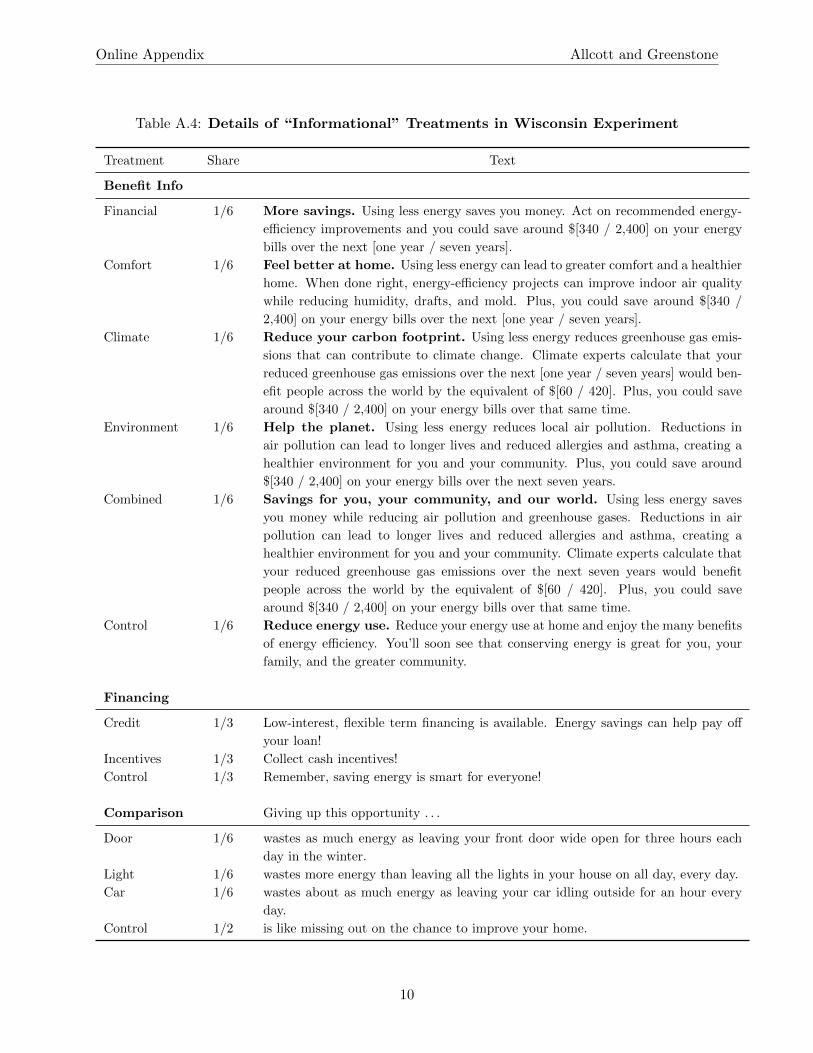
Online Appendix Allcott and Greenstone
Table A.4: Details of “Informational” Treatments in Wisconsin Experiment
Treatment Share Text
Benefit Info
Financial 1/6 More savings. Using less energy saves you money. Act on recommended energy-
efficiency improvements and you could save around $[340 / 2,400] on your energy
bills over the next [one year / seven years].
Comfort 1/6 Feel better at home. Using less energy can lead to greater comfort and a healthier
home. When done right, energy-efficiency projects can improve indoor air quality
while reducing humidity, drafts, and mold. Plus, you could save around $[340 /
2,400] on your energy bills over the next [one year / seven years].
Climate 1/6 Reduce your carbon footprint. Using less energy reduces greenhouse gas emis-
sions that can contribute to climate change. Climate experts calculate that your
reduced greenhouse gas emissions over the next [one year / seven years] would ben-
efit people across the world by the equivalent of $[60 / 420]. Plus, you could save
around $[340 / 2,400] on your energy bills over that same time.
Environment 1/6 Help the planet. Using less energy reduces local air pollution. Reductions in
air pollution can lead to longer lives and reduced allergies and asthma, creating a
healthier environment for you and your community. Plus, you could save around
$[340 / 2,400] on your energy bills over the next seven years.
Combined 1/6 Savings for you, your community, and our world. Using less energy saves
you money while reducing air pollution and greenhouse gases. Reductions in air
pollution can lead to longer lives and reduced allergies and asthma, creating a
healthier environment for you and your community. Climate experts calculate that
your reduced greenhouse gas emissions over the next seven years would benefit
people across the world by the equivalent of $[60 / 420]. Plus, you could save
around $[340 / 2,400] on your energy bills over that same time.
Control 1/6 Reduce energy use. Reduce your energy use at home and enjoy the many benefits
of energy efficiency. You’ll soon see that conserving energy is great for you, your
family, and the greater community.
Financing
Credit 1/3 Low-interest, flexible term financing is available. Energy savings can help pay off
your loan!
Incentives 1/3 Collect cash incentives!
Control 1/3 Remember, saving energy is smart for everyone!
Comparison Giving up this opportunity . . .
Door 1/6 wastes as much energy as leaving your front door wide open for three hours each
day in the winter.
Light 1/6 wastes more energy than leaving all the lights in your house on all day, every day.
Car 1/6 wastes about as much energy as leaving your car idling outside for an hour every
day.
Control 1/2 is like missing out on the chance to improve your home.
10

Online Appendix Allcott and Greenstone
Table A.5: Details of “Behavioral” and Subsidy Treatments in Wisconsin Experiment
Treatment Share Text
Graphical Prime
Financial 1/4 make BANK. Shrink your energy bills. Get paid.
CASH in. Save energy. Save money.
Environmental 1/4 earth LOVER. Save energy at home. Save the planet.
breathe EASY. Energy-efficient home. Cleaner air.
Climate 1/4 take CONTROL. Save energy. Reduce your carbon footprint.
PEACE of MIND. Energy-efficient home. Brighter future
Comfort 1/4 COMFY. Save energy. Live comfortably.
COZY. Feel better in your home.
Time Frame
Seven years 1/2 Example: “you could save around $2,400 on your energy bills over the next seven
years.”
One year 1/2 Example: “you could save around $340 on your energy bills over the next year.”
Audit Cue
Assessment 2/3 “home energy assessment”
Audit 1/3 “home energy audit”
Subsidy** Call to schedule a home energy [assessment/audit]. Usual cost: $400 ...
$100 Subsidy 0.06 You pay [nothing / only $200]!
$25 Subsidy 0.23 You pay only $[75 / 175]!
$25 Gift Card 0.20 You pay only $[100 / 200]! Bonus! Receive a $25 Visa Reward Card just for
completing an [assessment/audit]!
Control 0.51 You pay only $[100 / 200]!
**: These prices differed by city: the program subsidized the base price of audits (without the additionalexperimental subsidy) to $100 in Milwaukee and $200 in Madison.
11

Online Appendix Allcott and Greenstone
Figure A.5: Wisconsin Experiment Sample Letter 1
12

Online Appendix Allcott and Greenstone
Figure A.6: Wisconsin Experiment Sample Letter 2
13
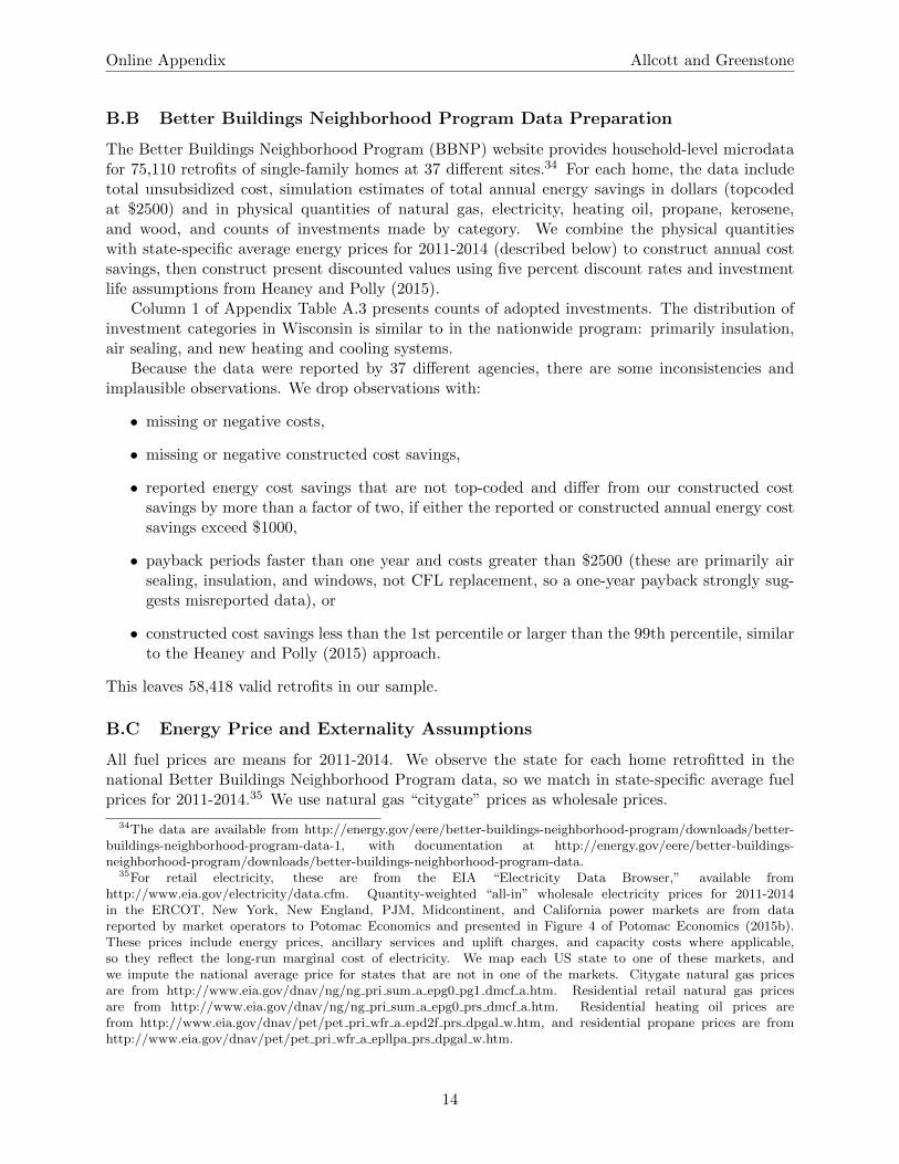
Online Appendix Allcott and Greenstone
B.B Better Buildings Neighborhood Program Data Preparation
The Better Buildings Neighborhood Program (BBNP) website provides household-level microdatafor 75,110 retrofits of single-family homes at 37 different sites.34 For each home, the data includetotal unsubsidized cost, simulation estimates of total annual energy savings in dollars (topcodedat $2500) and in physical quantities of natural gas, electricity, heating oil, propane, kerosene,and wood, and counts of investments made by category. We combine the physical quantitieswith state-specific average energy prices for 2011-2014 (described below) to construct annual costsavings, then construct present discounted values using five percent discount rates and investmentlife assumptions from Heaney and Polly (2015).
Column 1 of Appendix Table A.3 presents counts of adopted investments. The distribution ofinvestment categories in Wisconsin is similar to in the nationwide program: primarily insulation,air sealing, and new heating and cooling systems.
Because the data were reported by 37 different agencies, there are some inconsistencies andimplausible observations. We drop observations with:
• missing or negative costs,
• missing or negative constructed cost savings,
• reported energy cost savings that are not top-coded and differ from our constructed costsavings by more than a factor of two, if either the reported or constructed annual energy costsavings exceed $1000,
• payback periods faster than one year and costs greater than $2500 (these are primarily airsealing, insulation, and windows, not CFL replacement, so a one-year payback strongly sug-gests misreported data), or
• constructed cost savings less than the 1st percentile or larger than the 99th percentile, similarto the Heaney and Polly (2015) approach.
This leaves 58,418 valid retrofits in our sample.
B.C Energy Price and Externality Assumptions
All fuel prices are means for 2011-2014. We observe the state for each home retrofitted in thenational Better Buildings Neighborhood Program data, so we match in state-specific average fuelprices for 2011-2014.35 We use natural gas “citygate” prices as wholesale prices.
34The data are available from http://energy.gov/eere/better-buildings-neighborhood-program/downloads/better-buildings-neighborhood-program-data-1, with documentation at http://energy.gov/eere/better-buildings-neighborhood-program/downloads/better-buildings-neighborhood-program-data.
35For retail electricity, these are from the EIA “Electricity Data Browser,” available fromhttp://www.eia.gov/electricity/data.cfm. Quantity-weighted “all-in” wholesale electricity prices for 2011-2014in the ERCOT, New York, New England, PJM, Midcontinent, and California power markets are from datareported by market operators to Potomac Economics and presented in Figure 4 of Potomac Economics (2015b).These prices include energy prices, ancillary services and uplift charges, and capacity costs where applicable,so they reflect the long-run marginal cost of electricity. We map each US state to one of these markets, andwe impute the national average price for states that are not in one of the markets. Citygate natural gas pricesare from http://www.eia.gov/dnav/ng/ng pri sum a epg0 pg1 dmcf a.htm. Residential retail natural gas pricesare from http://www.eia.gov/dnav/ng/ng pri sum a epg0 prs dmcf a.htm. Residential heating oil prices arefrom http://www.eia.gov/dnav/pet/pet pri wfr a epd2f prs dpgal w.htm, and residential propane prices are fromhttp://www.eia.gov/dnav/pet/pet pri wfr a epllpa prs dpgal w.htm.
14

Online Appendix Allcott and Greenstone
For electricity and retail natural gas in the Wisconsin programs, we gathered marginal retailprices from staff at the Madison and Milwaukee utilities. Both utilities use time-invariant resi-dential electricity prices, except that Madison charges higher prices during the June-Septembersummer peak. We construct a consumption-weighted average price using 2011-2014 monthly aver-age electricity consumption data for Madison Gas and Electric reported on the EIA Form 826. Fornatural gas, both utilities have prices that vary by month. We construct consumption-weightedaverage retail prices using Wisconsin 2011-2014 monthly average retail natural gas consumptionfrom EIA.36 For citygate natural gas, wholesale electricity, and residential heating oil prices, weuse the Wisconsin data from the same EIA sources as for the national program.
Externality damage assumptions build primarily on Holland, Mansur, Muller, and Yates (2015),who graciously shared their data with us. Their key assumptions are a $6 million value of astatistical life and a fine particulate dose response function from Pope et al. (2002). We use a$39 social cost of carbon, based on estimates from the Interagency Working Group on the SocialCost of Carbon (2013) for 2013 and inflated to real 2013 dollars. For electricity, they provideestimates of average marginal damages by pollutant, NERC region, and hour. We weight the hoursby residential load shapes from the Integral Analytics DSMore model and sum across pollutants toget average marginal damages by state per kilowatt-hour conserved. Holland et al. also providedcounty-by-pollutant marginal damages for non-point sources, which are relevant for natural gasand heating oil combustion at places such as homes that do not have smokestacks. We inflate theseto 2013 dollars, collapse these to the state level, weighting by 2011 population, and multiply thestate average marginal damages by pollutant-specific emission factors for natural gas, heating oil,propane, kerosene, and wood from the AP-42 database (EPA 1995).
Drawing on Howarth et al. (2012) and Abrahams et al. (2015), we assume that three percentof natural gas leaks as methane during drilling and transportation before arriving in homes. Wetranslate this to carbon dioxide equivalents using a methane global warming potential of 34 fromthe Intergovernmental Panel on Climate Change (Myhre et al. 2013). This increases the naturalgas climate change externality by 38 percent, or $0.10/therm for residential natural gas.37
For heating oil sulfur content, we assume 2500 parts per million, except in Connecticut, Delaware,Maine, Massachusetts, New Hampshire, New Jersey, New York, and Pennsylvania, which are phas-ing in maximum fuel oil sulfur content regulations by 2018. In these states, we construct the presentvalue of average sulfur content over 2013-2032, using a five percent discount rate and maximumallowable fuel sulfur content reported by the New England Fuel Institute (2014). We assume thatmaximum fuel oil sulfur content restrictions larger than 2500 ppm are non-binding.
Appendix Table A.6 summarizes the energy price and externality assumptions. Climate exter-nality refers to carbon dioxide emissions, plus methane leakage for residential natural gas. Column1 presents averages for the Wisconsin experiment population. Retail gas and electricity prices differonly slightly between Madison and Milwaukee, and the table presents the average weighted by theshare of the audited population in each city. Column 2 presents averages across all households inthe national sample.
The table highlights three key issues. First, retail prices substantially exceed wholesale pricesfor both electricity and natural gas. Indeed, consistent with Davis and Muehlegger (2010), theretail natural gas markup more than exceeds the externality damages for the national programs,meaning that it may be optimal to tax investments that conserve natural gas. This is not the case
36This is available from http://tonto.eia.gov/dnav/ng/hist/n3010wi2m.htm.37Although this leakage also affects climate damages from electricity consumption, we do not include this because
our data from Holland, Mansur, Muller, and Yates do not include whether natural gas was on the margin. If naturalgas were on the margin 50 percent of the time, the electric power climate externality in Appendix Table A.6 wouldbe 38% × 50% × 2.3 cents/kWh ≈ 0.45 cents/kWh larger.
15
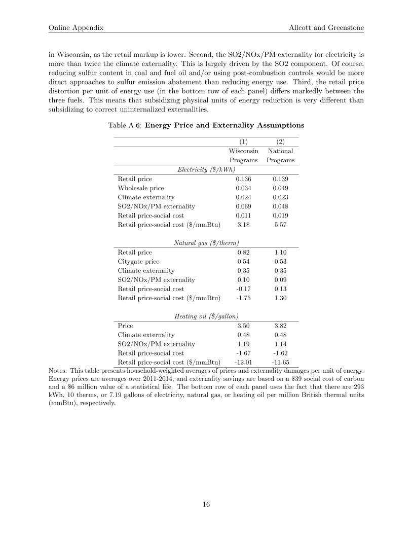
Online Appendix Allcott and Greenstone
in Wisconsin, as the retail markup is lower. Second, the SO2/NOx/PM externality for electricity ismore than twice the climate externality. This is largely driven by the SO2 component. Of course,reducing sulfur content in coal and fuel oil and/or using post-combustion controls would be moredirect approaches to sulfur emission abatement than reducing energy use. Third, the retail pricedistortion per unit of energy use (in the bottom row of each panel) differs markedly between thethree fuels. This means that subsidizing physical units of energy reduction is very different thansubsidizing to correct uninternalized externalities.
Table A.6: Energy Price and Externality Assumptions
(1) (2)
Wisconsin National
Programs Programs
Electricity ($/kWh)
Retail price 0.136 0.139
Wholesale price 0.034 0.049
Climate externality 0.024 0.023
SO2/NOx/PM externality 0.069 0.048
Retail price-social cost 0.011 0.019
Retail price-social cost ($/mmBtu) 3.18 5.57
Natural gas ($/therm)
Retail price 0.82 1.10
Citygate price 0.54 0.53
Climate externality 0.35 0.35
SO2/NOx/PM externality 0.10 0.09
Retail price-social cost -0.17 0.13
Retail price-social cost ($/mmBtu) -1.75 1.30
Heating oil ($/gallon)
Price 3.50 3.82
Climate externality 0.48 0.48
SO2/NOx/PM externality 1.19 1.14
Retail price-social cost -1.67 -1.62
Retail price-social cost ($/mmBtu) -12.01 -11.65Notes: This table presents household-weighted averages of prices and externality damages per unit of energy.Energy prices are averages over 2011-2014, and externality savings are based on a $39 social cost of carbonand a $6 million value of a statistical life. The bottom row of each panel uses the fact that there are 293kWh, 10 therms, or 7.19 gallons of electricity, natural gas, or heating oil per million British thermal units(mmBtu), respectively.
16

Online Appendix Allcott and Greenstone
C Appendix to Audit and Investment Takeup Estimates
Figure A.7: Private Internal Rate of Return and Investment Takeup in Wisconsin
0.1
.2.3
.4.5
.6.7
Tak
eup
rate
0.0
5.1
.15
Sha
re o
f rec
omm
ende
d in
vest
men
ts
-.2 0 .2 .4 .6Private Internal Rate of Return
Share Takeup Rate
Notes: Internal rates of return are computed at the 2011-2014 average retail natural gas and electricity pricesin the household’s city (Madison or Milwaukee). Subsidized costs are the upfront cost net of an imputedsubsidy of $500 per 10 percentage point projected decrease in the household’s pre-audit energy use. Theseare annualized IRRs, assuming that energy savings accrue in equal monthly installments until the end of theinvestment’s projected life.
17
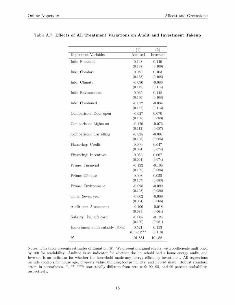
Online Appendix Allcott and Greenstone
Table A.7: Effects of All Treatment Variations on Audit and Investment Takeup
(1) (2)Dependent Variable: Audited Invested
Info: Financial 0.148 0.149(0.138) (0.109)
Info: Comfort 0.080 0.103(0.138) (0.108)
Info: Climate -0.090 -0.086(0.142) (0.114)
Info: Environment 0.035 0.148(0.140) (0.108)
Info: Combined -0.072 -0.034(0.142) (0.113)
Comparison: Door open -0.027 0.070(0.108) (0.083)
Comparison: Lights on -0.176 -0.076(0.112) (0.087)
Comparison: Car idling -0.025 -0.007(0.108) (0.085)
Financing: Credit 0.009 0.047(0.094) (0.074)
Financing: Incentives 0.050 0.067(0.094) (0.074)
Prime: Financial -0.122 -0.108(0.109) (0.086)
Prime: Climate 0.008 0.055(0.107) (0.083)
Prime: Environment -0.098 -0.099(0.108) (0.086)
Time: Seven year -0.002 -0.009(0.084) (0.066)
Audit cue: Assessment -0.100 -0.018(0.081) (0.064)
Subsidy: $25 gift card -0.005 -0.124(0.100) (0.081)
Experiment audit subsidy ($00s) 0.521 0.153(0.145)*** (0.118)
N 101,881 101,881
Notes: This table presents estimates of Equation (8). We present marginal effects, with coefficients multipliedby 100 for readability. Audited is an indicator for whether the household had a home energy audit, andInvested is an indicator for whether the household made any energy efficiency investment. All regressionsinclude controls for house age, property value, building footprint, city, and hybrid share. Robust standarderrors in parentheses. *, **, ***: statistically different from zero with 90, 95, and 99 percent probability,respectively.
18

Online Appendix Allcott and Greenstone
Table A.8: Tests of Whether Groups of Treatments Jointly Affect Takeup
(1) (2)
Dependent Variable: Audited Invested
Benefit info treatments 0.45 0.11
Comparison treatments 0.47 0.58
Graphical prime treatments 0.52 0.16
All “informational” treatments 0.63 0.24
All “behavioral” treatments 0.58 0.38
All non-subsidy treatments 0.67 0.24
Subsidy treatments 0.001 0.07
Notes: This table presents p-values of Wald tests of whether groups of coefficients in Appendix Table A.7jointly differ from zero. Audited is an indicator for whether the household had a home energy audit, andInvested is an indicator for whether the household made any energy efficiency investment.
19

Online Appendix Allcott and Greenstone
D Appendix to Estimates of Effects on Energy Use
D.A Additional Figures
Figure 5 combines event time estimates for natural gas and electricity. In this appendix, we presentthe separate estimates for each fuel. To parallel Appendix Table A.10 below, we also consider usingthe first investment date as the event, instead of the audit. Note that even in the post-investmentfigures, simulation model savings continue increasing (in absolute value) after month 0 becausethat month marks the first investment, which for many households is a “direct install” measureput in during the audit, and many of these same households later make larger investments througha contractor.
Appendix Figures A.8 and A.9 present the natural gas and electricity estimates underlyingFigure 5. In each figure, Panel (a) presents the estimates relative to the audit date, while Panel(b) presents the estimates relative to the first investment date. There are no significant pre-auditor pre-investment trends in either gas or electricity use. Immediately after the audit or investment,energy use decreases. By the end of the first year post-audit, natural gas usage averages 0.09therms/day lower, and electricity usage averages about 1.6 kWh/day lower. Relative to pre-auditaverages of 2.40 therms/day and 21.4 kWh/day, these represent approximately four and sevenpercent reductions.
Relative to the empirical estimates, the simulations predict much larger natural gas savings,both post-audit and post-investment. By contrast, the empirical estimates for post-audit elec-tricity savings are much larger than predicted, and the post-investment estimates are noisy andindistinguishable from the prediction. Note that although Eit = 0 for all t before the audit, thecoefficient estimates are not exactly zero before the audit and investment due to the inclusion ofmonth-of-sample effects µm.
Appendix Figures A.10 and A.11 present analogues to Appendix Figures A.8 and A.9, exceptlimiting the sample to a “balanced” set of households whose energy bills are observed over the entireevent window of 18 months before to 18 months after. (For the investment figures, households thatmade no investments are also included as controls.) This eliminates the possibility of compositionaleffects, i.e. that systematically different sets of households would identify treatment effects fordifferent months. The “balanced” group of households turns out to have made larger investments:on average, they were projected to save 17 percent more gas and 36 percent more electricity thanthe non-balanced group by the end of the first year post-audit. Thus, the energy savings in FiguresA.10 and A.11 are somewhat larger than for the full sample. Otherwise, the figures look verysimilar.
Appendix Figures A.12 and A.13 present analogues to Figures A.10 and A.11, except over ashorter time window. Because these figures limit to the “balanced” set of households observed overthe entire window in order to eliminate compositional effects, limiting to a smaller window allowsus to include additional households that are observed only over a shorter period. This and othertime windows all give essentially the same pictures as Figures A.10 and A.11.
Appendix Figure A.14 presents the audit event studies for households with no recorded in-vestments. Again, there are no discernible pre-trends. The point estimates suggest a slight butimprecisely-estimated post-audit increase in natural gas use.
20
Online Appendix Allcott and Greenstone
Figure A.8: Natural Gas Usage in Event Time
-1-.
8-.
6-.
4-.
20
.2N
atur
al g
as u
sage
(th
erm
s/da
y)
-20 -10 0 10 20Months after audit
Empirical estimate Simulation prediction
(a) Post-Audit
-1-.
8-.
6-.
4-.
20
.2N
atur
al g
as u
sage
(th
erm
s/da
y)
-20 -10 0 10 20Months after first investment
Empirical estimate Simulation prediction
(b) Post-InvestmentNotes: This figure presents energy use in event time relative to the household’s audit or investment. Dashedlines are 90 percent confidence intervals. Mean pre-audit natural gas usage is 2.40 therms/day.
21

Online Appendix Allcott and Greenstone
Figure A.9: Electricity Usage in Event Time
-3-2
-10
1E
lect
ricity
usa
ge (
kWh/
day)
-20 -10 0 10 20Months after audit
Empirical estimate Simulation prediction
(a) Post-Audit
-3-2
-10
1E
lect
ricity
usa
ge (
kWh/
day)
-20 -10 0 10 20Months after first investment
Empirical estimate Simulation prediction
(b) Post-InvestmentNotes: This figure presents energy use in event time relative to the household’s audit or investment. Dashedlines are 90 percent confidence intervals. Mean pre-audit electricity usage is 21.4 kWh/day.
22

Online Appendix Allcott and Greenstone
Figure A.10: Natural Gas Usage in Event Time in Balanced Sample
-1-.
8-.
6-.
4-.
20
.2N
atur
al g
as u
sage
(th
erm
s/da
y)
-20 -10 0 10 20Months after audit
Empirical estimate Simulation prediction
(a) Post-Audit
-1-.
8-.
6-.
4-.
20
.2N
atur
al g
as u
sage
(th
erm
s/da
y)
-20 -10 0 10 20Months after first investment
Empirical estimate Simulation prediction
(b) Post-InvestmentNotes: This figure presents energy use in event time relative to the household’s audit or investment. Dashedlines are 90 percent confidence intervals. Mean pre-audit natural gas usage is 2.40 therms/day. This parallelsFigure A.8 but includes on the “balanced” sample of households.
23

Online Appendix Allcott and Greenstone
Figure A.11: Electricity Usage in Event Time in Balanced Sample
-3-2
-10
1E
lect
ricity
usa
ge (
kWh/
day)
-20 -10 0 10 20Months after audit
Empirical estimate Simulation prediction
(a) Post-Audit
-3-2
-10
1E
lect
ricity
usa
ge (
kWh/
day)
-20 -10 0 10 20Months after first investment
Empirical estimate Simulation prediction
(b) Post-InvestmentNotes: This figure presents energy use in event time relative to the household’s audit or investment. Dashedlines are 90 percent confidence intervals. Mean pre-audit electricity usage is 21.4 kWh/day. This parallelsFigure A.9 but includes on the “balanced” sample of households.
24

Online Appendix Allcott and Greenstone
Figure A.12: Natural Gas Usage in Event Time in Balanced Sample over Shorter Win-dow
-1-.
8-.
6-.
4-.
20
.2N
atur
al g
as u
sage
(th
erm
s/da
y)
-15 -10 -5 0 5 10Months after audit
Empirical estimate Simulation prediction
(a) Post-Audit
-1-.
8-.
6-.
4-.
20
.2N
atur
al g
as u
sage
(th
erm
s/da
y)
-15 -10 -5 0 5 10Months after first investment
Empirical estimate Simulation prediction
(b) Post-InvestmentNotes: This figure presents energy use in event time relative to the household’s audit or investment. Dashedlines are 90 percent confidence intervals. Mean pre-audit natural gas usage is 2.40 therms/day. This parallelsFigure A.10 but covers a shorter time window.
25

Online Appendix Allcott and Greenstone
Figure A.13: Electricity Usage in Event Time in Balanced Sample over Shorter Window
-3-2
-10
1E
lect
ricity
usa
ge (
kWh/
day)
-15 -10 -5 0 5 10Months after audit
Empirical estimate Simulation prediction
(a) Post-Audit
-3-2
-10
1E
lect
ricity
usa
ge (
kWh/
day)
-15 -10 -5 0 5 10Months after first investment
Empirical estimate Simulation prediction
(b) Post-InvestmentNotes: This figure presents energy use in event time relative to the household’s audit or investment. Dashedlines are 90 percent confidence intervals. Mean pre-audit electricity usage is 21.4 kWh/day. This parallelsFigure A.11 but covers a shorter time window.
26
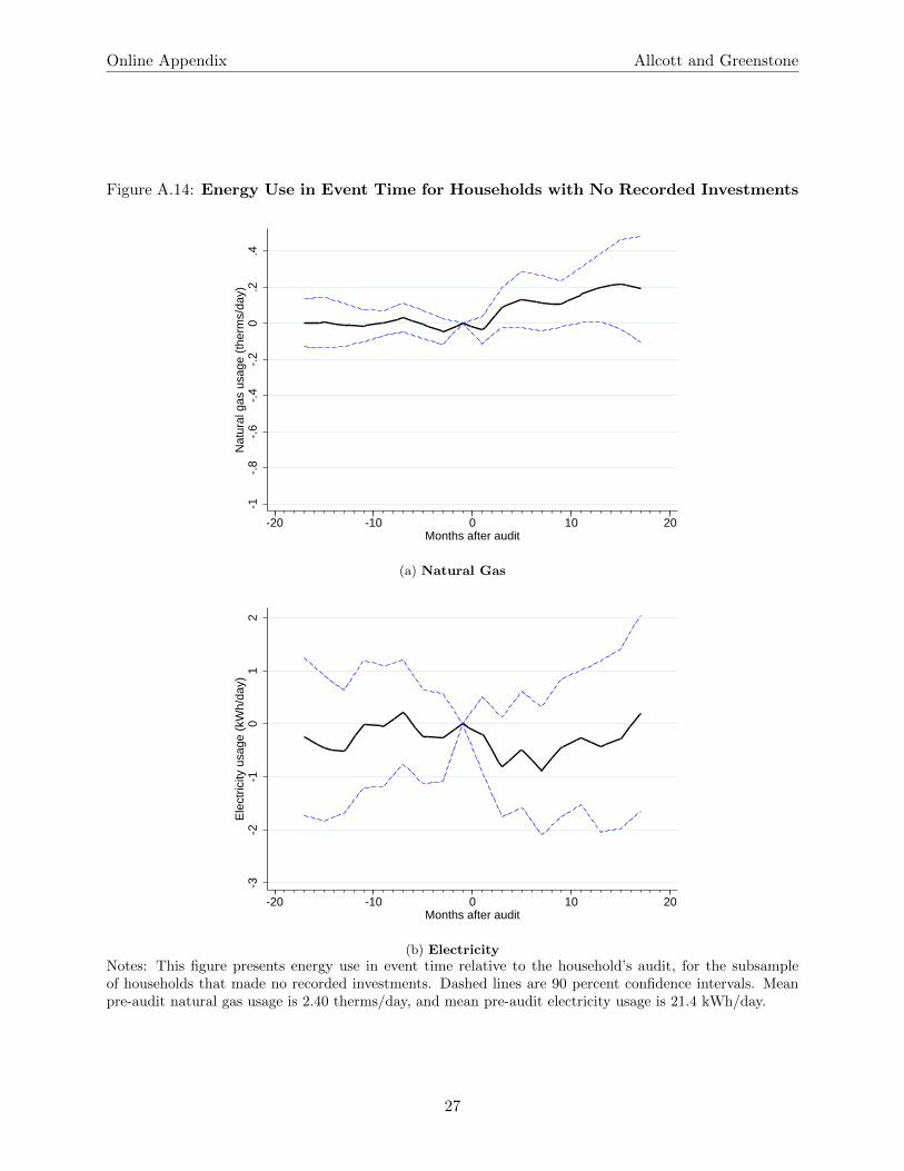
Online Appendix Allcott and Greenstone
Figure A.14: Energy Use in Event Time for Households with No Recorded Investments
-1-.
8-.
6-.
4-.
20
.2.4
Nat
ural
gas
usa
ge (
ther
ms/
day)
-20 -10 0 10 20Months after audit
(a) Natural Gas
-3-2
-10
12
Ele
ctric
ity u
sage
(kW
h/da
y)
-20 -10 0 10 20Months after audit
(b) ElectricityNotes: This figure presents energy use in event time relative to the household’s audit, for the subsampleof households that made no recorded investments. Dashed lines are 90 percent confidence intervals. Meanpre-audit natural gas usage is 2.40 therms/day, and mean pre-audit electricity usage is 21.4 kWh/day.
27
Online Appendix Allcott and Greenstone
D.B Extensions to Table 6
Appendix Table A.9 presents robustness checks and extensions to Table 6. As with Table 6, columns1 and 2 present natural gas estimates, while columns 3 and 4 present electricity estimates. Columns1 and 3 limit the sample to households that made no observed investments, paralleling AppendixFigure A.14. Three of the four coefficients on the post audit indicators are statistically insignificant,which would suggest that these households do not make significant unobserved investments. Fornatural gas, however, the coefficient on Post audit (≥6 months) is positive and significant with 90percent confidence.38
Columns 2 and 4 repeat columns 1 and 3 of Table 6, except with weather-unadjusted simulationestimates as the dependent variable. The estimates are similar to but slightly smaller than theestimates using weather-adjusted predictions. This implies that the post-audit and post-investmentsamples include slightly more extreme temperatures, in which more savings would be expectedrelative to prediction. The ≥ 6 month gas realization rate using the weather-unadjusted resultsin column 3 is -0.128/-0.409≈31 percent. For comparison, the weather-adjusted figure reported inFigure 6 was 29 percent.
In the body of the paper, we defined Pit as a pair of post-audit indicators, estimating theeffects of audits plus subsequent investments. Appendix Table A.10 parallels Table 6, except addingpost-investment indicators to Pit. Recall that Eit takes value 0 before investments are made andequals the predicted savings thereafter. Many households audited but did not invest, so the post-audit indicators from Table 6 represent a diluted effect of investments in the larger populationof households that audited. In Appendix Table A.10, the predicted post-investment savings nowload more heavily onto the post-investment indicators. There are small decreases associated withthe post-audit indicators in column 3 due to the combination of minor compositional effects withmonth of sample dummies µm.
These results can be used to construct an alternative realization rate based on the post-investment coefficients. The natural gas realization rate is 0.458/1.036≈44%, while the electricityrealization rate is 0.199/0.836≈24%. When combined at retail prices, this gives an over realizationrate of 42 percent.
The main interesting feature of this table is that the electricity savings in column 4 are muchmore strongly associated with the post-audit indicators than the post-investment indicators. Thissuggests that the excess electricity savings may not be attributable to the observed investments,which in any event are largely projected to save natural gas. Instead, the excess savings could resultfrom unobserved actions taken after the audit, such as additional CFL installation and appliancereplacement, that would not be recorded in the programs’ administrative data. When adjustingthe accounting welfare analysis in Section VIII for empirically-realized savings, we assume thatthe excess electricity savings accrue because of the observed investments, which may cause us tounderstate total investment costs for the empirically-estimated energy savings. This biases againstour finding that program costs outweighed benefits.
To better understand the differences between the simulation and empirical estimates, we con-struct a “shortfall” variable Yit−Eit, measuring the difference between actual usage and predictedsavings. Columns 1 and 3 of Appendix Table A.11 regress this shortfall on the interaction ofpost-audit indicators with indicators for whether the household made made one of the three most
38Additional regressions show that this apparent post-audit gas use increase is unlikely to be driven by unobservedenergy efficiency investments: the increase is no larger at households that received recommendations of new heatingand cooling systems or water heaters. The increase is unlikely to be driven by substitution from electricity to gas:post-audit gas use changes are not associated with electricity use changes. We do find that the apparent usage increaseis limited to only above-median natural gas users. Our best guess is that the apparent increase is an idiosyncraticresult for a subset of heavy users where the difference-in-differences controls are imperfect.
28
Online Appendix Allcott and Greenstone
common investments: insulation, heating/cooling, and “other,” which includes air sealing, newwater heaters, new windows, pipe and duct sealing and insulation, and programmable thermostats.Positive coefficients mean that the investment is associated with a savings shortfall, while negativecoefficients mean that the investment is associated with excess savings. Column 1 shows that insu-lation and heating/cooling are not statistically significantly associated with the shortfall variable,although the t-statistic on insulation is around 1.3. By contrast, natural gas shortfalls are statisti-cally significantly associated with investments in the “other” category. (We do not have sufficientpower to further disaggregate the “other” category.) Consistent with our results, a recent report bythe TREAT model developers (PSD 2015b) also finds that air sealing and insulation predictions areimportant contributors to low realization rates. The TREAT model is “in close alignment with thepredictions from best-in-class modeling tools” (PSD 2015b), so this finding may be more generalthan just TREAT.
Columns 2 and 4 add an indicator for whether a new appliance appears in the household’slist of recommended measures. The program’s takeup data do not include appliances becausethey were not subsidized, but the fact that this last interaction is significant suggests that thesehouseholds may have reduced both natural gas and electricity use through unobserved appliancepurchases. However, only 25 households in the energy use data were recommended appliances, sothis is not enough to fully explain the excess post-audit electricity savings relative to the simulationpredictions.
See Blasnik (2010), Nadel and Keating (1991), and PSD (2015b) for more in-depth discussionsof why simulations can systematically overestimate empirically-realized savings. One broad classof explanations has to do with the assumptions and parameters used by the program and itsauditors. For example, a home’s baseline energy use could be overstated, giving excess simulatedsavings. This explains most of the empirical shortfall in the PSD (2015b) New York study. Inthe Wisconsin programs, however, only 12 percent of pre-audit observations were calibrated withestimates instead of the audited household’s true baseline energy use, so this particular factor seemsunlikely to explain much of the our estimated shortfall.39 Another factor that could cause excesssimulated savings in Wisconsin and elsewhere is that simulations often assume best-case installationscenarios that could not be realized except through great effort by the most expert contractors.This, or any other source of systematic bias, can be addressed (on average) by scaling back allpredictions by some factor less than one.
39The default calibrations were 23 percent lower and 12 percent higher than the average audited household’spre-audit usage of gas and electricity, respectively.
29

Online Appendix Allcott and Greenstone
Table A.9: Post-Audit Energy Use Changes: Alternative Estimates
(1) (2) (3) (4)Natural Gas (therms/day) Electricity (kWh/day)
Non- Weather- Non- WeatherInvestors’ Unadjusted Investors’ UnadjustedEnergy Simulation Energy Simulation
Dependent Variable: Use Prediction Use Prediction
Post audit (<6 months) 0.068 -0.225 -0.416 -0.292(0.043) (0.021)*** (0.395) (0.025)***
Post audit (≥6 months) 0.112 -0.409 -0.145 -0.402(0.057)* (0.029)*** (0.524) (0.034)***
N 22,455 61,845 23,098 63,655
Notes: This table presents alternative estimates of Equation (12). Columns 1 and 3 present estimatesfor households with no recorded investments. Columns 2 and 4 present estimates of Equation (12) withweather-unadjusted simulation predictions as the dependent variable. Mean pre-audit natural gas usage is2.40 therms/day, and mean pre-audit electricity usage is 21.4 kWh/day. Average marginal natural gas priceis $0.82 per therm, and average marginal electricity price is $0.136 per kWh. All columns control for heatingand cooling degrees, household-by-calendar month fixed effects, and month-of-sample fixed effects. Robuststandard errors in parentheses, clustered by household. *, **, ***: statistically different from zero with 90,95, and 99 percent probability, respectively.
30

Online Appendix Allcott and Greenstone
Table A.10: Post-Investment Energy Use Changes
(1) (2) (3) (4)Natural Gas (therms/day) Electricity (kWh/day)
Simulation Energy Simulation EnergyDependent Variable: Prediction Use Prediction Use
Post audit (<6 months) 0.010 0.016 -0.082 -0.796(0.021) (0.030) (0.019)*** (0.259)***
Post audit (≥6 months) 0.013 0.067 -0.045 -0.918(0.022) (0.037)* (0.023)** (0.340)***
Post investment (<6 months) -0.849 -0.323 -0.626 -0.217(0.030)*** (0.030)*** (0.037)*** (0.293)
Post investment (≥6 months) -1.036 -0.458 -0.836 -0.199(0.031)*** (0.037)*** (0.052)*** (0.345)
N 61,845 61,845 63,655 63,654
Notes: This table presents estimates of Equation (12) with daily usage of natural gas and electricity, re-spectively, as the dependent variables, using data from the Wisconsin experiment. This parallels Table 6,except adds post-investment indicators. Columns 1 and 3 have the simulation predictions as the dependentvariable, while columns 2 and 4 have energy use as the dependent variable. Mean pre-audit natural gasusage is 2.40 therms/day, and mean pre-audit electricity usage is 21.4 kWh/day. Average marginal naturalgas price is $0.82 per therm, and average marginal electricity price is $0.136 per kWh. Robust standarderrors in parentheses, clustered by household. *, **, ***: statistically different from zero with 90, 95, and99 percent probability, respectively.
Table A.11: Associations of Energy Savings Shortfalls with Specific Investments
(1) (2) (3) (4)Natural Gas (therms/day) Electricity (kWh/day)
Post audit × Insulation 0.179 0.158 -0.997 -1.265(0.140) (0.138) (1.454) (1.356)
Post audit × Heating/cooling -0.003 0.004 -0.518 -0.432(0.064) (0.064) (0.539) (0.534)
Post audit × Other 0.348 0.367 1.373 1.607(0.142)** (0.140)*** (1.489) (1.393)
Post audit × Recommended appliance -0.219 -3.255(0.069)*** (0.879)***
N 61,845 61,845 63,654 63,654
Notes: This table presents alternative estimates of Equation (12), interacting Pit with indicators for installedand recommended investment categories. The dependent variable is Yit −Eit, the difference between actualusage and predicted savings. Mean pre-audit natural gas usage is 2.40 therms/day, and mean pre-auditelectricity usage is 21.4 kWh/day. Average marginal natural gas price is $0.82 per therm, and averagemarginal electricity price is $0.136 per kWh. All columns control for heating and cooling degrees, household-by-calendar month fixed effects, and month-of-sample fixed effects. Robust standard errors in parentheses,clustered by household. *, **, ***: statistically different from zero with 90, 95, and 99 percent probability,respectively.
31

Online Appendix Allcott and Greenstone
D.C Can the “Rebound Effect” Explain the Empirical Shortfall?
We present two calculations to test whether the “rebound effect,” i.e. increased utilization inresponse to a decreased cost of energy services, can explain the low natural gas realization rate.For this section, we use the realization rate implied by the post-investment coefficients in TableA.10, which is 0.458/1.036≈44%. Since this is slightly higher than the realization rate from thepost-audit coefficients, our calculations are “conservative”: it would be even more difficult for therebound effect to explain the lower post-audit realization rate.
First, we calculate the price elasticity of demand for energy services that would be implied if allof the empirical shortfall is due to increased utilization. The change in quantity of energy serviceswould be
%∆qenergy services =Actual Post-Investment Usage
Simulated Post-Investment Usage− 1 ≈ 0.419. (15)
The change in price of energy services is
%∆penergy services =Simulated Usage Reduction
Baseline Usage≈ −0.429. (16)
The implied elasticity is thus
%∆qenergy services%∆penergy services
≈ −0.98. (17)
A utilization elasticity of -0.98 appears to be unrealistically large in this population. For com-parison, the most closely-related estimates of energy utilization elasticity are much smaller: -0.06,-0.3, and -0.22 for washing machines (Davis 2008), home electricity (Dubin and McFadden 1984),and autos (Gillingham 2014), respectively.
The second calculation is to determine the change in indoor temperature that would be requiredto generate the entire empirical shortfall. To do this, we make two assumptions. First, we assumethat natural gas consumption is a linear function of the difference between indoor and outdoortemperatures. Second, we assume that households keep indoor temperatures constant as outdoortemperatures fluctuate, or more weakly that indoor temperatures are not conditionally correlatedwith outdoor temperatures. Under these two assumptions, we can estimate the natural gas requiredto increase indoor temperatures using variation in outdoor temperatures. We estimate the followinganalogue to Equation (12):
Yit = ιPitWit + ω(1− Pit)Wit + νi + µm + εit. (18)
where Yit is natural gas consumption, Pit is a post-investment indicator, Wit is heating andcooling degrees, νi is a household-by-calendar month fixed effect, and µm are month-of-sampleindicators. The coefficient ι measures natural gas consumption as a function of the differencebetween indoor and outdoor temperatures.
In the post-investment sample, we estimate ι ≈ 0.035 therms/cooling degree and ι ≈ 0.099therms/heating degree. If 1/3 of the year in Wisconsin requires cooling and 2/3 of the year requiresheating, then the average therms per degree of indoor temperature per day is 1
3 · 0.035 + 23 ·
0.099 ≈ 0.078. Comparing the ≥ 6 month post-investment simulation vs. empirical estimatesin columns 2 vs. 4 of Table 6 gives an empirical shortfall of 1.036 − 0.458 ≈ 0.578 therms/day.Thus, to explain the full empirical shortfall, indoor temperatures would have to change (increase inwinter and decrease in summer) by 0.589/0.078 ≈ 7.5 degrees. This would be unrealistically large.
32

Online Appendix Allcott and Greenstone
For comparison, Fowlie, Greenstone, and Wolfram (2015) find no statistically significant post-weatherization temperature change in a low-income (and thus likely more price elastic) populationin Michigan. They can reject a post-weatherization temperature change of more than 1.4 degreeswith 90 percent confidence in a two-sided test.
In summary, the “rebound effect” is likely to explain only a small fraction of the empiricalshortfall for natural gas.
33

Online Appendix Allcott and Greenstone
E Accounting Welfare Analysis of National Better Buildings Pro-gram
It is important to know whether our results in Table 7 are specific to the Wisconsin programs,or whether they generalize more broadly. To test whether the Wisconsin experimental samplewas somehow unusual, we augment the analysis with microdata from all Better Buildings pro-grams nationwide, representing $435 million in upfront costs across 58,418 households at 37 sites.We downloaded the data from the DOE website and prepared the data according to the processdescribed in Appendix B.B.
Table A.12 describes data from the 37 Better Buildings Neighborhood Program sites that re-ported to the Department of Energy. These data are more limited than for the Wisconsin programs:for each household retrofitted through the program, we observe the categories of investments made(as in Wisconsin, typically insulation, air sealing, and heating and cooling), total (unsubsidized)cost, and simulation estimates of total annual energy savings in physical units. The primary twofuels saved are electricity and natural gas, but the data also include predicted savings of heating oil,propane, kerosene, and wood. We group these latter four fuels as “other fuels” for Table A.13. Wetranslate physical units to dollars and externality reductions using the same process described inSection IV, with data from the state and electricity market where the site is located. Of the 75,110households in the original data, 58,418 survive the data cleaning process described in Appendix B.
Table 7 presents welfare effects using the “accounting approach.” Columns 1 and 2 replicateTable 7, presenting results for the Wisconsin programs, while columns 3 and 4 present the na-tionwide BBNP results.40 Columns 1 and 3 use the simulation predictions to calculate energy andexternality reductions. Column 2 multiplies the Wisconsin simulation estimates by realization ratesof 2.48 for electricity and 0.29 for natural gas and other fuels, on the basis of Table 6 and Figure6. Column 4 multiplies the national program simulation estimates by realization rates of 0.59 forelectricity and 0.47 for natural gas and other fuels, on the basis of the DOE’s (2015c) nationalBBNP evaluation.
Under the assumptions of the accounting approach, the programs reduce welfare. Even using thesimulation predictions, the Wisconsin and national programs have benefit/cost ratios of 0.92 and0.75 at five percent discount rates, with internal rates of return of 4.0 and 1.5 percent, respectively.After adjusting for the empirical shortfall, the benefit/cost ratios are 0.43 and 0.38, and the IRRsare negative 4.1 and negative 5.2 percent. The projects from the national program with valid datainvolved total cost of $435 million, compared to empirically-adjusted social benefits of $166 million.
Of course, the results of the engineering approach depend on energy price and externalityassumptions. For empirically-adjusted benefits to exceed costs, energy acquisition costs wouldneed to be 4.2 and 3.9 times larger, all externality damages would need to be 3.3 and 4.7 timeslarger, or the social cost of carbon would need to be $239 and $301 per ton for the Wisconsin andnational samples, respectively.
The U.S. Department of Energy (DOE) has conducted an official evaluation of the nationwideBetter Buildings Neighborhood Program (DOE 2015c). The DOE report evaluates BBNP as aneconomic stimulus program, which is relevant given that it was funded through the AmericanRecovery and Reinvestment Act, but does not present a benefit-cost analysis relevant for typicalmacroeconomic conditions. By contrast, we do not consider the economic stimulus benefit, so whileour analysis is appropriate under normal economic conditions, we are not evaluating whether the
40We assume that the unsubsidized audit cost is cA = $400, based on typical market prices. The national BetterBuildings program dashboard reports a grand total of 138,323 single-family home audits and 74,493 retrofits. Applyingthat 54 percent follow-through rate implies that 108,474 audits were required to generate the 58,418 valid projectsin our data.
34

Online Appendix Allcott and Greenstone
programs increased welfare during the Great Recession. The DOE’s headline benefit/cost ratio of3.0 is the ratio of economic activity created (i.e. private sector expenditures plus tax revenues)divided by federal government outlays. This calculation is not comparable to ours. Indeed, it ismechanically opposite: energy efficiency investment costs count as a cost in our framework, whilethey count as a benefit in the DOE framework because they represent additional economic stimulus.The details of the DOE report suggest that if they had done an analysis like ours, they would havearrived at similar conclusions: total program costs exceed retail energy savings plus carbon emissionbenefits, and their empirical analysis finds a 52 percent realization rate for residential retrofits aftercombining electricity and gas.41
Table A.12: Summary Statistics for National Better Buildings Program Data
Variable Mean Std.
Dev.
Min. Max.
Total cost ($) 6705 5711 100 30,000
Retail energy cost savings ($/year) 472 430 12.7 2734
Notes: Sample size is the 58,418 households that made investments and survive the data cleaning processdescribed in Appendix B. Energy prices are averages over 2011-2014; see Appendix B for details.
41The DOE evaluation reports $669 million in lifetime bill savings and $972 million in total costs, plus 7.2 millionmetric tons of CO2 abated, which sums to $274 million at a $39 social cost of carbon. In this sense, costs exceedbenefits by $29.4 million. However, this is not directly comparable to our benefit-cost analysis, because it considersenergy savings at retail prices instead of avoided costs, uses undiscounted future energy and environmental benefits,and does not include the local air pollution benefits.
35

Online Appendix Allcott and Greenstone
Table A.13: Welfare Effects: Accounting Approach, Including National Programs
(1) (2) (3) (4)
Wisconsin Programs National Programs
Simulation Empirically Simulation Empirically
Source of energy savings estimates: Predictions Adjusted Predictions Adjusted
Cost ($millions)
Audit costs (at $400 per audit) 0.56 43
Investment costs 4.52 392
Total cost 5.08 435
Energy Savings ($millions present value at 5% discount rate)
Natural gas 1.92 0.56 77 36
Electricity 0.07 0.18 43 25
Other fuels 0.61 0.18 68 32
Total 2.61 0.92 187 93
Externality Reduction ($millions present value at 5% discount rate)
Climate (at $39 per ton CO2) 1.37 0.57 81 40
SO2/NOx/PM 0.72 0.68 59 32
Total 2.09 1.26 140 73
Summary
Benefits - Costs ($millions) -0.39 -2.91 -108 -270
Benefit/Cost ratio 0.92 0.43 0.75 0.38
Internal rate of return (percent) 4.0 -4.1 1.5 -5.2
Notes: Columns 1 and 2 present estimates for the Wisconsin sample, and Columns 3 and 4 present estimatesfor the 58,418 households that invested under the national Better Buildings program and have valid data.Columns 1 and 3 use energy savings projected by simulation models, while columns 2 and 4 adjust forempirically-observed savings. Column 2 multiplies electricity and gas/other fuels savings from Column 1 by2.48 and 0.29, respectively, based on the estimates in Table 6. Column 4 multiplies electricity and gas/otherfuels savings from Column 3 by 0.59 and 0.47, respectively, based on estimates from DOE (2015c). Energysavings are calculated at average wholesale prices over 2011-2014, and externality reductions are based on a$39 social cost of carbon and a $6 million value of a statistical life; see Appendix B for details.
36
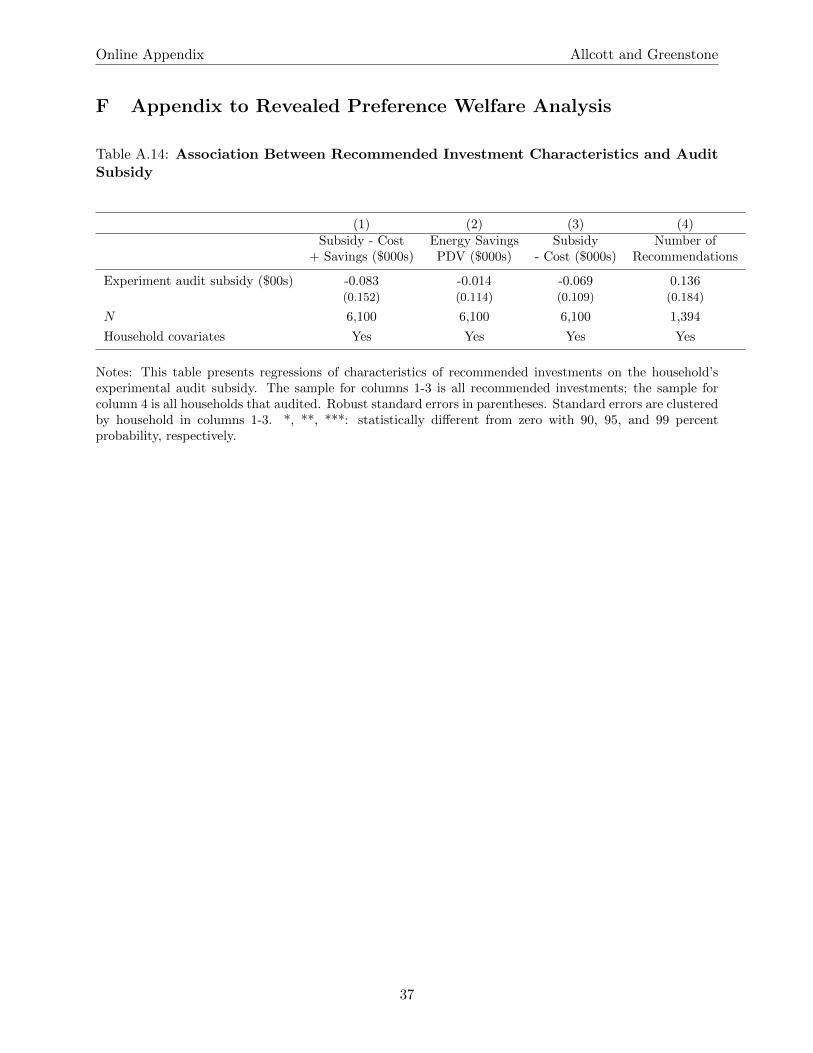
Online Appendix Allcott and Greenstone
F Appendix to Revealed Preference Welfare Analysis
Table A.14: Association Between Recommended Investment Characteristics and AuditSubsidy
(1) (2) (3) (4)Subsidy - Cost Energy Savings Subsidy Number of
+ Savings ($000s) PDV ($000s) - Cost ($000s) Recommendations
Experiment audit subsidy ($00s) -0.083 -0.014 -0.069 0.136(0.152) (0.114) (0.109) (0.184)
N 6,100 6,100 6,100 1,394
Household covariates Yes Yes Yes Yes
Notes: This table presents regressions of characteristics of recommended investments on the household’sexperimental audit subsidy. The sample for columns 1-3 is all recommended investments; the sample forcolumn 4 is all households that audited. Robust standard errors in parentheses. Standard errors are clusteredby household in columns 1-3. *, **, ***: statistically different from zero with 90, 95, and 99 percentprobability, respectively.
37
References
[1] Heaney, Michael, and Ben Polly (2015). “Analysis of Installed Measures and Energy Savings for Single-Family Residential Better Buildings Projects.” National Renewable Energy Laboratory Technical Re-port 5500-64091 (April).
[2] Myhre, G., D. Shindell, F.-M. Breon, W. Collins, J. Fuglestvedt, J. Huang, D. Koch, J.-F. Lamarque,D. Lee, B. Mendoza, T. Nakajima, A. Robock, G. Stephens, T. Takemura and H. Zhang. 2013. “An-thropogenic and Natural Radiative Forcing.” In: Climate Change 2013: The Physical Science Basis.Contribution of Working Group I to the Fifth Assessment Report of the Intergovernmental Panel onClimate Change [Stocker, T.F., D. Qin, G.-K. Plattner, M. Tignor, S.K. Allen, J. Boschung, A. Nauels,Y. Xia, V. Bex and P.M. Midgley (eds.)]. Cambridge University Press, Cambridge, United Kingdomand New York, NY, USA.
[3] New England Fuel Institute (2014). “State Sulfur & Bioheat Requirements for No. 2 Heating Oil inthe Northeast & Mid-Atlantic States.” Available from http://www.nefi.com/news/docs/heating-oil-standards-chart.pdf. Accessed June 12, 2015.
[4] Potomac Economics (2015b). “2014 State of the Market Re-port for the ERCOT Wholesale Electricity Markets.” Available fromhttps://www.potomaceconomics.com/uploads/ercot documents/2014 ERCOT State of the Market Report.pdf.Accessed August 18, 2015.
38
Recommended