MPRAMunich Personal RePEc Archive

The Welfare Effects of Social Mobility:An Analysis for OECD countries.

Fischer, Justina AV

OECD

02. September 2009

Online at http://mpra.ub.uni-muenchen.de/17070/

MPRA Paper No. 17070, posted 02. September 2009 / 16:58

1

The Welfare Effects of Social Mobility:

An Analysis for OECD countries

Justina A.V. Fischer+

OECD Paris.

Version 2 Sept 2009

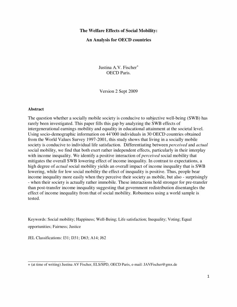
Abstract

The question whether a socially mobile society is conducive to subjective well-being (SWB) has

rarely been investigated. This paper fills this gap by analyzing the SWB effects of

intergenerational earnings mobility and equality in educational attainment at the societal level.

Using socio-demographic information on 44’000 individuals in 30 OECD countries obtained

from the World Values Survey 1997-2001, this study shows that living in a socially mobile

society is conducive to individual life satisfaction. Differentiating between perceived and actual

social mobility, we find that both exert rather independent effects, particularly in their interplay

with income inequality. We identify a positive interaction of perceived social mobility that

mitigates the overall SWB lowering effect of income inequality. In contrast to expectations, a

high degree of actual social mobility yields an overall impact of income inequality that is SWB

lowering, while for low social mobility the effect of inequality is positive. Thus, people bear

income inequality more easily when they perceive their society as mobile, but also - surprisingly

- when their society is actually rather immobile. These interactions hold stronger for pre-transfer

than post-transfer income inequality suggesting that government redistribution disentangles the

effect of income inequality from that of social mobility. Robustness using a world sample is

tested.

Keywords: Social mobility; Happiness; Well-Being; Life satisfaction; Inequality; Voting; Equal

opportunities; Fairness; Justice

JEL Classifications: I31; D31; D63; A14; J62

________________________________________ + (at time of writing) Justina AV Fischer, ELS/SPD, OECD Paris, e-mail: JAVFischer@gmx.de

Acknowledgement

The author thanks Andrew Clark, Henrik Jordahl, Alois Stutzer, and colleagues from the OECD

such as Simon Chapple, Enrico Giovannini, Maria Huerta del Carmen, and Mark Pearson, for

helpful comments and suggestions. This paper was first written when the author was working in

the Social Policy Division (ELS) at the OECD, and builds on a previous version entitled “Social

Mobility and Subjective Well-Being”, ELS/SPD, February 2009, and an internal working party

document of the ELS/SPD presented in October 2008. This project has been financed by the EU

Commission which had no influence on its design, analysis, interpretation or decision to submit.

This version replaces all previous versions.

The views expressed in this paper are those of the authors alone, not necessarily of the OECD or

any of its Member countries.

3

1. Introduction

1.1. Background and aim of paper: Democracy and social mobility

There is the tendency and the observation in the Western World to view democratic political

structures as well as social mobility and equality in opportunities as two inseparable dimensions

of socio-economic and societal progress – a progress at least the majority of the population

should profit from.1

Approximating the unobserved utility experienced by one person using survey-based self-report

measures of subjective well-being (SWB),2 the welfare impacts of democratic political decision-

making and impartiality of decisions of the government administration have been well

investigated. While Dorn et al. (2007) identify a positive association between the extent of civil

and political liberties and individual welfare, a positive linkage of government efficiency and a

strong rule of law with population well-being is reported in Helliwell and Huang (2007) and

Bjørnskov, Dreher and Fischer (2008c). However, there is a research gap of analyses on the

welfare effects of social mobility as a characteristic of society.

1.2. Previous, related literature

Most of previous evidence of the welfare effects of social mobility in society, either actual or

perceived, has been only indirect. Alesina, DiTella and MacCulloch (2004) use a perceived

social mobility argument to explain the differential impacts of income inequality on individual

1 Since the 20th century, in Economics societal progress has been equated with growth in national income (GDP).

For recent attempts to re-define societal progress and to develop alternative measures focusing on a quality

dimension, see the discussion in e.g. OECD (2007). One approach is to use indicators of subjective well-being

(SWB) – which is employed in this paper.

2 See Dolan, Peasgood, and White (2008) for a recent survey of happiness research. In this paper, we use the notions

‘life satisfaction’, ‘happiness’, ‘subjective well-being’ (SWB), and ‘well-being’ interchangeably, given that they

all proxy utility, but being aware of their conceptional differences. Discussion of these differences would go

beyond the scope and purpose of this paper (see Fischer, 2009).

SWB between the US and Western Europe. In particular, they relate the insignificant effect of

income dispersion in the US to prospects of upward mobility, while linking the negative impact

in Western Europe to social immobility. In a similar vein, Senik (2008) compares the effects of

reference income, the income level on which social comparisons are based on, across Western

and Eastern European countries. She explains the beneficial, SWB increasing effects in the post-

communist countries with a rising-income-trajectory argument. Potentially, the positive,

beneficial reference income effects at the neighborhood level, with simultaneously negative,

SWB decreasing comparison income effects at the national level, reported in Kingdon and

Knight (2007), may equally be explained by differences in (perceived) social mobility: while

neighbours’ income level may play a role model for their own (upward) income expectations, the

national reference income may merely yield negative social comparisons effects. Social mobility

effects at the individual level are assessed by Clark and D’Angelo (2008). Comparing the type of

job held by parents with that occupied by their child, the impact of a personal intergenerational

improvement on individual SWB is clearly positive. Taken all together, these studies provide

only indirect evidence, sometimes only conjectures, on the effects of socially mobile society on

well-being. Indeed, direct empirical evidence on the subjective well-being effects of social

mobility, as nature of the society an individual lives in, is still lacking.

1.3. Topic of paper

This paper addresses the question whether a socially mobile society is conducive to societal and

individual welfare, also taking into account its interplay with income inequality. Extending

previous analyses, not only perceived, but also actual social mobility is analyzed; in addition,

income distribution before and after redistributive government activities are differentiated.

In this paper we define social mobility as intergenerational improvement in income or social

status, comparing the parental generation’s standing with one’s own (contrasting intra-

generational changes that relate to the identical individual).3 In this study, social mobility in

3 As the concept of social mobility implies contrasting individual social status with social status of the preceding

generation, it is somewhat related to the field of ‘social comparisons’ or ‘relative deprivation’, which assumes a

5

society is captured by two direct measures: one that relates to average intergenerational earnings

dependence in society, while the second assesses the average dependence of student’s education

attainment on their family background. In principle, both measures are not restricted to upwards

mobility only, but available for OECD countries only. Notably, due to the cross-sectional nature

of the social mobility and happiness data employed, causality cannot be inferred from a

methodological point of view, which leaves room for further explorations when international

micro-macro-panels become available.

1.4. Outline of paper

The rest of the paper is organized as follows: section 2 introduces the data and provides

descriptive statistics, while the subsequent section briefly discusses the method of statistical

analysis. Section 4 analyzes the SWB models and presents the results for actual and perceived

social mobility, also taking account of heterogeneity by respondent’s political ideology. In

section 5 the models test the effects of income inequality and its interplays with perceived and

social mobility. Section 6 provides further-reaching, more speculative discussions of the

empirical findings, while section 7 summarizes and concludes.

comparison of individual’s income with a certain contemporaneous threshold income, e.g. average income. For a

literature overview, see, e.g., Clark and Oswald (1996), Ferrer-i-Carbonell (2005), Fischer and Torgler (2008). For

a thorough empirical assessment of relative and absolute income effects on happiness, see Ferrer-i-Carbonell

(2005).

2. Data

2.1. Micro data on SWB

Using the World Values Survey (WVS) data from 1997 to 2001 for the subsample of 30 OECD

countries, we extract information on 44’000 persons. Subjective well-being is measured using

the life satisfaction question, which asks , “All things considered, how satisfied are you with

your life as whole these days ? ”, and rates its answers on a 10-point scale, ranging from

“completely dissatisfied” to “completely satisfied”. These data have been previously employed

in numerous scientific articles written by economists, sociologists and political scientists, and

focuses on the cognitive, evaluative component of subjective well-being in a broader sense (e.g.,

Bjørnskov, Dreher and Fischer, 2008a, 2008b; Helliwell and Huang, 2007). For the country-level

analyses, the population share of those responding in the highest three categories is employed

(following e.g. Bjørnskov, Dreher, and Fischer, 2007), while the micro-level analysis exploits the

full scale of the life satisfaction question.

2.2. Measures of actual social mobility

This paper addresses the question whether living in a society with more social mobility is

conducive to SWB. In this paper we define social mobility as intergenerational improvement in

income or social status, comparing the parental generation’s standing with one’s own

(contrasting intragenerational changes that relate to the identical individual). Thus, in a society

with equal opportunities we should observe wages and earnings which are less dependent on

family background and parental income (Roemer, 2002). Already at school, student performance

should be less determined by parental education level.

2.2.1. Intergenerational earnings elasticity

To measure the degree of social mobility in society, two measures are employed: first, the

intergenerational earnings elasticity, which measures the dependence of one’s own life-time

7

income to parental income, based on a father-son comparison.4 The earnings elasticity in this

study is obtained from estimating a model in which son’s log earnings is a function of log of

father’s earnings, usually also correcting for life-cycle bias, based on the theoretical framework

developed by Becker and Tomes (1979). The estimated coefficient represents then

intergenerational earnings elasticity. In all OECD countries, this coefficient takes on positive

values ranging from 0.15 to 0.5 which reflect smaller and larger intergenerational persistence, on

average. The extreme value of 0 indicates complete generational mobility, with no relation

between parent and child outcomes, while the maximum value of 1 reflects complete immobility.

A value of 0.5 implies that 50% of father’s earnings advantage is passed on to his son. According

to Corak (2006), even small values can indicate substantial earnings differences by parental

background: e.g. for the US, an elasticity of 0.4 implies that adult children of high-income

parents earn more than two-and–a-half higher incomes compared to descendents of low-income

parents (in case of 0.2, the income advantage is still 1.64). This earnings elasticity measure is,

however, only available for 12 countries in our sample. The data are obtained from OECD

(2008), which summarizes the meta-studies by D’Addio (2007) (3 countries) and Corak (2006)

(9 countries), which present elasticities corrected for various biases (e.g. measurement errors due

to natural income fluctuations) and made cross-nationally comparable. To ease interpretation of

the empirical findings, elasticity estimates have been multiplied with -1 so that higher values

indicate more social mobility in the labor market. In our sample, the least mobile countries are

United Kingdom (-0.5), Italy (-0.48), and the USA (-0.47); the most socially mobile OECD

countries in our sample are Denmark (-0.15) and Norway (-0.17) (see Table 1).

4 Ideally, elasticity would be based on both parents’ income and their female and male childrens’ incomes, with

elasticity measuring “the fraction of income differences between two parents that, on average, is observed among

their children in adulthood” (Corak, 2006). However, due to low female labor force participation rates in the

parental generation, longitudinal data on female parental incomes is still largely missing, so that estimated

intergenerational wage elasticity would be unreliable.

2.2.2. Mobility in educational attainment

The second measure assesses social mobility in society before the labor market entry takes place,

namely at the education stage. Intergenerational transmission of education is often captured by a

measure of dependency of student’s educational attainment of her parents’ education. Available

for this study are mobility measures based on PISA 2003 student performance data in

Mathematics and the information on family background. More precisely, educational mobility is

approximated by the difference between the mean student test score in the high-education-

family-background-subsample and that in the medium-level-of-parental-education-subsample.

This difference in means is calculated for mother’s and father’s education background separately

(but does not differentiate by student’s gender). To ensure cross-national comparability, levels of

parental education are measured on the international, standardized ISCED scale, with level 3

(upper secondary education) representing the medium level of parental education and levels 5 or

6 (completed tertiary education) reflecting the highest level in this comparison. For example, in

Spain, the mean test score of students with mothers who have a completed tertiary education is

514 points, while that for students whose mothers have an upper secondary education, the

medium level of parental education, is only 489. Thus, a higher-education background

(compared to a medium level of education-background) yields an average advantage of 514 - 489

= 25 test score points (see Table 1), a quarter of a standard deviation of the PISA test scores.5

These differences are calculated for 29 OECD countries based on the PISA 2003 scores in

Mathematics, obtained from OECD (2004) and OECD (2007).

To ease interpretation of this mobility measure, its values have been multiplied with -1 so that

higher values reflect more mobility in terms of intergenerational dependency of educational

attainment. With respect to maternal education level (and excluding Mexico as outlying

observation)6, this recoded measure ranges between -57.74 and 2.41 PISA test score points, with

negative values indicating educational immobility, as the educational advantage persists over

generations. Values close to zero imply that, on average, both student subsamples by parental

5 The standardized international mean is 500 test score points with a standard deviation of 100 points.

6 The value of 20.14 points for Mexico indicates some considerable downward mobility in terms of educational

attainment for those with an educationally advantageous family background.

9

education perform equally well, indicating that family background plays no role for student

attainment. 7

Table 1shows that highly immobile countries (in terms of maternal education level)

are all Eastern European OECD countries (Poland: -53.94 points, Czech Republic: -54.27 points,

Hungary: -57.74 points, Slovak Republic: -48.59 points), while most mobile are Italy (-1.28

points), Portugal (-1.7 points), Sweden (-2.59 points), and Switzerland (2.41 points).

-------------------------------------------

Insert Table 1 about here

-------------------------------------------

2.3. Measures of perceived social mobility

In the course of this analysis, an approximate measure of perceived social mobility is employed,

constructed using three questions of the WVS. The questions account for confidence in one’s

country’s education system, the belief that it is possible to escape from poverty, and that poverty

is caused by laziness and lack of will, as opposed to bad luck. The latter two WVS questions

have been used by Alesina, Glaeser and Sacerdote (2001) to motivate the differences in

perceived social mobility between the US and Western Europe. A person is defined as perceiving

her society as socially mobile if she responds positively to at least one of three questions.

Altogether, this procedure yields a social mobility perception measure for 30’000 individuals in

25 OECD countries, with the confidence in education measure clearly dominating.8 Thus, this

measure builds largely on the idea that education is an important determinant of socio-economic

position, and that equal opportunities in education generate socio-economic mobility, which is

empirically supported for a small sample of developed countries by the meta-study of Corak

(2006). However, one may argue that intergenerational mobility in education does not reflect

overall social mobility, be it actual or perceived. For reasons of robustness, a more narrow

7 Alternatively, education mobility in terms of years of education could have been employed. However, the duration

may just reflect the efficiency of the schooling or education system. In addition, it is not outcome-focused.

8 The confidence in education measure is available for 21 countries, the remaining two measures for three countries

(AUS, NOR, NZL).

definition of perceived social mobility is employed, which is based only on the latter two

questions excluding the education aspect, but which is available for fewer countries and

individuals. All mobility and national income measures are taken from the OECD databases and

the publication ‘Society at a Glance, 2006’ (OECD, 2007).

2.4. Other control variables at the country level

In various robustness tests, we employ the Net National Income per capita (NNI, in its log form),

which approximates the level of disposable income in the population, and social trust in the

population.9 Social trust at the societal level is measured as the population share of yes-

respondents to the World Values Survey question “Generally speaking, would you say that most

people can be trusted or that you need be very careful in dealing with people?”. Table 1 lists the

values of the actual social mobility (three measures), the perceived social mobility (population

mean), the corresponding GINI coefficients, and subjective well-being (population share of

happiest) for 30 OECD countries.

3. Methodology

Correlation analyses have been carried out at the country level, with individual-level information

aggregated to the societal level, giving rise to 30 data points. A first robustness test with respect

to national income and social capital is carried out, both applying OLS and robust regressions

(RR) that take account of potential outliers in the sample.10

9 NNI is defined as GDP plus wages, earnings, salaries and property income earned abroad, minus the depreciation

of fixed capital assets. NNI is a more accurate measure of economic well-being of the population compared to

GDP.

10 In a robust regression, first, any observation is excluded that has a Cook’s D value of greater than 1, and second,

based on the absolute size of previous-round residuals, observations are assigned weights from 0 to 1.

11

The second and core part of this paper applies multi-level multivariate regressions exploiting the

variation across individuals as well as across countries in the data. Combining individual-level

information with country characteristics, we obtain a cross-section to which we apply weighted

OLS, with clustering by countries to take account of within-group correlations. In particular, this

technique corrects for the fact that actual social mobility as measured (as well as income

inequality) varies only across countries, so that the standard errors of these macro estimates are

correctly calculated.

The application of OLS to a categorical dependent variable (life satisfaction) can be justified

based on Ferrer-i-Carbonell and Frijters (2004). They show that using OLS in place of ordered

probit in SWB analyses preserves the direction of the effects, the significance levels of the

coefficient estimates as well as their relative importance. Using OLS has also the advantage that

coefficients can directly be interpreted as marginal effects, and that interaction terms are

meaningful, so that total (marginal) effects can easily be calculated. Coefficients in OLS

regressions relate to changes in categories of life satisfaction.11

4. Results

4.1. Country-level analysis

4.1.1. Simple correlations between happiness in population and social mobility

We start with investigating simple country-level correlations between SWB in the population and

social mobility. Actual social mobility is measured either by the (recoded) elasticity of one’s

own wage to parental income or approximated by the (recoded) deviation of student performance

in PISA 2003 with a high-education family background from that of medium-education

background, so that higher values correspond with more social mobility. As the following

11 In contrast, marginal effects calculated based on ordered probit estimates relate to changes in probability of

reporting a certain (pre-determined) SWB category.

Graphs 1 and 2 suggest, actual social mobility shows the expected positive correlations with

subjective well-being in OECD countries. The correlation coefficients are ρ = 0.75, 0.49, and

0.45, respectively, indicating that stronger intergenerational dependence of economic success

lowers societal well-being. 12

------------------------------------------------

Insert Graphs 1 and 2 about here

-------------------------------------------------

4.1.2. Testing for alternative explanations: national wealth and trust

It may be argued that the positive correlation between social mobility and SWB are driven by

unobserved factors: national wealth, or, alternatively, social trust. Countries that are socially

more mobile should allocate human capital more efficiently, and, in the long-run, grow faster

and reach higher levels of national wealth.13

This parallel development is reflected in the so-

called modernization hypothesis of societal progress. On the other hand, social trust may well

12 Referring to the introduction of this paper, equal opportunities may also be approximated by more economic

freedom and civil participation possibilities, e.g. measured by the Gastil index of civil liberties

(www.freedomhouse.org). Also for this measures of social mobility we find strong positive correlations with

SWB at the country level, ρ = 0.64. On the other hand, social mobility may also be linked to government

interventions that correct ‘unfair’ market outcomes. For OECD countries, we find a strong positive relation

between confidence in the social security system and SWB (ρ = 0.46). Indeed the importance of fairness

perceptions for SWB has been analyzed in e.g. Tortia (2008).

13 For example, in Western Europe, (proto-)industrialization was made possible through the deliberate destruction of

the medieval feudal system (manoralism), allowing for geographical mobility and land reform, introduction of

economic freedom, and destruction of the craft gild system (England: 1660/ 1760, France: 1789-1793, Prussia:

1807/1810/1866), allowing for entrepreneurship, price competition between manufactures, technological progress,

and performance-based pay schemes. A similar linkage between industrialization and social mobility can be

observed in Russia under Tzar Peter I (the Great, 1682 - 1725), whose reforms included not only state support for

foundation of private enterprises, but also modernization of government administration and state control of the

church. Another example is Japan in 1854, the year the harbours were re-opened to foreign goods and knowledge

after centuries of isolation, accompanied by the deliberate abolition of the Japanese (semi-)feudal system in

1871/1877 by emperor Mutsuhito (1867 – 1912). For literature, see e.g. Encyclopaedia Britannica (2009).

13

constitute a pre-condition for a socially mobile society. Social trust is the general belief that one

treats each other in a fair, non-abusive manner (Bjørnskov, 2007; Jordahl, 2007). As social

mobility implies unpredictable shifts of bargaining power across groups and individuals, a

trusting and trustworthy environment may protect the individual against the adverse effects of

social mobility.14

Uslaner (2008) suggests that social trust is a rather time-invariant feature of

society, transmitted through the family line. Thus, social mobility may just approximate national

wealth or social trust, but not exert an impact of its own.

The correlations between NNI per capita (as of 2000) and the social mobility measures are as

expected for mobility in education (ρ = 0.25; ρ = 0.37) (but not for intergenerational wage

mobility, ρ = 0.03), while the correlation of NNI with SWB is positive and significant (ρ =

0.59).15

Thus, living in a rich country goes along with having more equal educational

opportunities. National wealth may also be associated with and thus approximate the quality of

government institutions. The correlations of log(NNI) with measures of government

effectiveness (Kaufman et al., 2008), the rule of law (Fraser Institute), and the absence of

perceived corruption (Transparency International) exceed ρ = 0.66.16

The positive correlation

coefficients between these institutional quality measures and the social mobility indicators reveal

that better institutions are found in more socially mobile societies. For intergenerational wage

14 That other-regarding fairness considerations put a constraint on purely self-regarding behaviour has been shown in

experimental economics, e.g. in so-called one-shot dictator distribution games in which non-sharing cannot not be

punished by the receiver (Fehr and Schmidt, 1999). Bergren and Jordahl (2008) claim that economic freedom in

society lets social trust emerge; in this line, social mobility would trigger social trust, equally giving rise to their

positive correlation.

15 The correlation with NNI (2000) with intergenerational earnings elasticity is ρ = 0.03, with maternal and paternal

education-dependence of student performance ρ = 0.25 and ρ = 0.37, respectively.

16 The correlation coefficients are ρ = 0.86, 0.66, and 0.73, respectively.

mobility, these correlations exceed 0.5, while for the educational mobility measures, they show

the same tendency, but are smaller in size.17

4.1.3. Partial correlations between inequality and SWB in the population using OLS and RR

To account for this correlation structure, multivariate regressions using OLS and RR for 30

OECD countries are carried out, with country’s SWB as dependent variable, and as explanatory

factors the log of NNI, social trust, and our mobility measure of interest.18

Table 2 reports the

results for the SWB effects of social mobility when also national income is controlled for, while

Table A3 of the Appendix adds to the model social trust in society.

In Table 2, we also report the coefficient estimates for the unconditional association between

social mobility and national happiness, applying the same weights. The similarity of the

conditional with the unconditional social mobility coefficient (mostly staying significant)

suggests that unobserved national wealth does not drive our previous results. Obviously,

providing social mobility that may reflect equal opportunities, which is beneficial to SWB, is not

a question of a country’s financial resources. According to Table 2, an increase in social mobility

in terms of intergenerational wage elasticity by 0.1 increases the share of happiest persons in

society by 6 percentage points. Similarly, an increase in educational attainment independence by

10 test score points increases the happy population share by 6.6 percentage points. The

regressions for social trust yields the coefficients for mobility in education unchanged. In

contrast, the coefficient on social mobility in terms of intergenerational earnings elasticity, which

is only available for 12 countries, appears reduced in size, but stays jointly significant. Thus, the

SWB effects of mobility in the labor market are partly mediated by social trust, which is not the

case for educational mobility. Possibly, actual earnings are more decisive determinants of one’s

17 Correlations coefficients with recoded wage elasticity are ρ = 0.5, 0.68, and 0.72, respectively, and with recoded

dependency on mothers (father’s) educational background ρ = 0.2 (0.26), 0.08 (0.12), and ρ = 0.25 (0.26),

respectively.

18 Adding NNI to models 3 to 6 increases the adjusted R2 from roughly 0.2 to above 0.4, indicating a considerably

better model fit.

15

socio-economic positions in society than is education. Nevertheless, both mobility measures stay

influential.

Taken altogether, the social mobility effects for SWB do not appear to account for unobserved

country characteristics such as social trust and national income.

-------------------------------------------

Insert Table 2 about here

-------------------------------------------

4.2. Main specification: Societal versus individual social mobility

Analogous analyses of the individual SWB effects of living in a mobile society using a combined

micro-macro-level approach are carried out, in which individual-level characteristics are

combined with country-specific factors (e.g. Bjørnskov, Dreher and Fischer (2008a, 2008b). This

approach exploits the variation in subjective well-being across individuals, while the variation of

factors at the country level remains the same. The full model includes controls for gender, age,

marital status, education, income, denomination, political ideology and various facets of social

capital, alongside with national income. As described in the methodology section, OLS with

observations clustered at the country level is applied to account for within-group correlation.

Table A2 provides descriptive statistics of the individual-level determinants.

4.2.1. SWB effects of social mobility

Table 3 shows that social mobility in society exerts a well-being raising influence, as does

national income. In the full models (columns 1 and 3), the marginal effects of intergenerational

labor market mobility and mobility in educational attainment are 1.33 and 0.012 - 0.017,

respectively, indicating the happiness gain from a one-unit increase in the explanatory variable.

Consequently, moving from a completely immobile (-1) to a completely mobile society (0) in

terms of earnings would, ceteris paribus and causally interpreted, increase an individual’s well-

being by more than one satisfaction category (1.33), on average. More feasible in reality is a

move from the (recoded) maximum wage persistence in our OECD sample (-0.5, e.g. UK) to

maximum mobility (-0.15, Denmark), that would yield a happiness gain by half of a SWB

category. For educational mobility, a decrease of parental background advantage by 50 test score

points (maximum in sample: -57 points) would increase life satisfaction by more than 2/3 of a

category, on average. Assessment of the relative importance of social mobility effects is

achieved through comparison with the marginal effects for the control variables in a baseline

model reported in Table A2 of the Appendix. The SWB effects of about 2/3 of a category or

more - triggered by considerable changes in social mobility - are only comparable to associations

with SWB (in absolute terms) of being in a medium-to-high income category compared to being

in the lowest income category (yielding happiness gains of about 70% to 99% of a category), or

being unemployed compared to being full-time employed (-80% of a category). SWB effects of

half of a category are still quite sizable and are similar in size to e.g., having a medium-level

income (compared to the lowest income), or being married.19

Comparably large impacts are also

observable for the log of national income, as Table 3 suggests (60% - 100% of a SWB category,

depending on the model specification).

4.2.2. The relation between socio-demographic characteristics and mobility in society

Stronger results for earnings mobility are observable when only gender and age, the only truly

exogenous individual-specific determinants, are employed (columns 2, 4, and 6). Compared to

the full model 1, which employs all individual-level controls, the coefficient size of

intergenerational earnings elasticity appears larger in absolute terms (1.33 vs. 1.69, representing

an increase by 30%), suggesting that parts of its effects are captured by choice-driven individual-

specific characteristics as education and income. In this light, the significant effect of social

mobility in the full model is particularly noteworthy, suggesting that social mobility at the

societal level and social mobility experienced as past personal history are distinct.

19 As Table A2 of the Appendix shows, sizes of most of the significant OLS coefficient estimates on determinants of

SWB in 30 OECD countries do not exceed the value of 0.35 in absolute terms.

17

This observation of differential marginal effects across model specifications is not made for

social mobility in educational attainment, for which almost all coefficients remain unaffected by

the inclusion of potentially endogenous micro-level control variables (e.g. column 3 versus

column 4). This similarity in coefficients on intergenerational education dependency across

model variants remains in the smaller sample for the intergenerational wage elasticity variable.

4.2.3. The relation between mobility in the labor market and in education

Labor market mobility in society has a different effect on SWB according to whether individual

income is excluded or included in the model. In contrast, for intergenerational mobility in

educational attainment no such observation is made: the coefficient estimate on education

mobility is insensitive to the inclusion of respondent’s education, income, and occupational

status. A possible explanation is that equality in educational opportunity does not fully transmit

into equality of opportunities in the labor market.

Breen (2004) suggests that in countries with a policy of providing equal educational

opportunities soft skills that are not learned at school but in the family may well gain in

importance for obtaining certain occupational positions and for career opportunities. Indeed, the

correlation coefficients between labor market mobility and education mobility are low and

sensitive to the number of countries included in the sample: the small negative correlation in the

full sample (ρ = -0.4) disappears when Italy is excluded, yielding no correlation (ρ = -0.08).20

This is in accordance with the estimates of Table 3 that suggest that there is no direct causal

chain from educational mobility to income and occupation.

What are the mechanisms responsible for this counterintuitive finding ? Traditionally,

sociologists’ and economists’ empirical analyses of social mobility (‘social fluidity’) suggest that

education plays an important role for social class destination. In particular, education was shown

to be a decisive mediating factor for the impact of class origin on class destination (class origin

20 Please note that the positive correlation in Corak (2006) is based on a much smaller sample and partly less precise

measures.

=> education => class destination). Intuitively, it may be appealing to think that by increasing

educational mobility, overall social mobility will be increased. However, the empirical analyses

presented in Breen (2004) show that between 1970 and 2000 social mobility has not converged

at all in 11 European countries (including Israel) and cross-national variation remains substantial.

In addition, it is argued that educational mobility and meritocratic principles need to be changed

simultaneously in order to achieve a higher overall social mobility: Breen (2004) states that a

policy to increase enrolments in higher education with a view to increasing social mobility will

not be effective if this also changes the degree to which segmented labor markets operate on a

meritocratic basis. Indeed, as more people get better educated, the origin-class-destination-class-

link at these higher levels of education might even strengthen (as shown by Vallet, 2004, for

France). In such case, speaking with Corak (2006), social connections, family culture, as well as

the preferences and goals among children formed by the family may become decisive for success

in the labor market, leading to the opposite policy effect than the intended one, causing lower

social mobility.21

In addition, the extent of the effect of educational mobility on social mobility

also depends on the strength of the link between education level and class destination, which

varies greatly across countries.

-------------------------------------------

Insert Table 3 about here -------------------------------------------

In the later part of this paper, the question of the linkage between mobility in educational

attainment and mobility in the labor market will be discussed again.

21 For literature on changes in educational mobility in industrialized countries (associations between class origin and

educational attainment), see Breen and Jonsson (2005). Notably, for the USA, several studies report no decrease

in educational inequality.

19

4.3. Political ideology

4.3.1. Left-wing oriented persons

Traditionally, leftist oriented persons are believed to prefer equal outcomes, e.g. low degrees of

inequality. Such equalization of outcome may well be realized by government interventions that

favour the disadvantaged and socially marginalized, e.g. through redistribution of market

incomes through taxation and welfare transfers. However, a more equal distribution of market-

generated earnings is also believed to be achieved by equalization of levels of educational

attainment, making educational attainment independent of parental background and breaking up

the linkage between parental generation income inequality and the present generation income

distribution (see OECD 2008, p.216). Low social mobility can reinforce income inequality

driving its continuing increase over time (see OECD 2008 p.214 and p.27). In this view, social

mobility in terms of labor market outcomes can be viewed as indication that that poverty

transmission across generations has successfully been broken up: “if the degree of

intergenerational transmission of disadvantage can be reduced, the aptitudes and abilities of

everyone in society are more likely to be used efficiently, thus promoting both growth and

equity" (OECD 2008, p.214). Thus, social mobility may, in the long run, be conducive to equity.

That leftist oriented persons are inequality averse to a stronger degree compared to conservative

persons has been shown by e.g. Alesina et al. (2004) for both the US and Western Europe. While

there is no direct empirical evidence on the linkage between preferences for social mobility and

political orientation, Clark et al. (2008) suggest a positive linkage between own-experienced

individual upward-mobility and being leftist. Specifically, they have shown that persons with an

improved socio-economic status in the labor market, compared to that of their parents, measured

by the Goldthorpe index, are more likely to be pro-redistribution, pro-public sector and vote for

leftist parties. This finding does not contradict that socio-economic status per se is positively

associated with being conservative (empirically supported by Piketty 1995, Persson and Tabellini

1996, Alesina and La Ferrara 2005), this being controlled for in the modelling.22

22 This finding contradicts their intuitive prediction that social climbers would express a more conservative political

ideology, aiming at not having to share their newly gained property with the ‘have-nots’. As their findings are

In sum, improving social mobility should be in accordance with leftists’ policy goals,

contributing to their subjective well-being.23

4.3.2. Right-wing oriented persons

On the other hand, as argued by Alesina and La Ferrara (2005), a conservative view-point may

well be in line with a belief that market outcomes are performance-based, and thus ‘fair’,

opposing too great a degree of income redistribution. Similarly, Clark and D’Angelo (2008)

argue that individuals will be more conservative the higher their own social upward-mobility

(having achieved a higher socio-economic position compared to their parents’ standing).24

Indeed, Alesina and La Ferrara (2005) show that believing in ‘hard work’ as main factor for

getting ahead is associated with a preference for less redistribution in the US. Using individual

data from the General Social Survey, they also report a negative association between having a

personal history of upward mobility in the labor market and preferences for redistribution.25

Also

derived from the British Household Panel, the observed linkages between own past mobility and political self-

positioning may well be specific to the British culture.

23 Based on these arguments, social mobility should be negatively correlated with income inequality, possibly

stronger with market-generated pre-transfer income inequality than with inequality in disposable income after

corrective redistribution through the government. However, correlations of social mobility in the labor market

with pre- and post-transfer income inequality of mid-2000 are rather comparable in size (ρ = -0.69 and -0.71,

respectively) (see also OECD (2008), p.13 for Gini coefficients based on disposable income (ρ = -0.68)). In

contrast, correlations between mobility in educational attainment and market income inequality of mid-2000 are

not significant, while being significantly negatively correlated with final income inequality (when Italy is

excluded as outliers). Possibly, mobility in educational attainment captures population preferences for equalizing

market outcomes. See also Table A9.

24 Corneo and Gruener (2002) argue that due to growing heterogeneity in milieu and rising probabilities of matches

with persons from a low-class family background in the marriage market, high-income persons are more likely to

oppose social mobility and income redistribution.

25 Social mobility is measured as the intergenerational difference in job prestige. Notably, for social mobility

proxied by the difference in years of education a pro-redistribution effect is observable, controlling for individual

level of education. See also Alesina and Angeletos (2002) and Fong (2001) for similar findings.

21

Corneo and Gruener (2002) identify a linkage between (subjectively perceived) upward mobility

and the call for less redistributive activities for 7000 persons from 12 developed, mostly OECD

countries. Higher social mobility would then be interpreted as a stronger personal achievement

reflection of socio-economic status, and being in line with conservative political preferences.26

Taken altogether, favoring social mobility may be in accordance with a rightwing political

ideology, and be conducive to subjective well-being of politically conservative persons.

4.3.3. Empirical Analysis: Social mobility effects for SWB by political ideology

To analyze the heterogeneity of SWB effects of social mobility in society by political ideology,

Table 4 estimates the full model that includes all socio-demographic controls for two ideology-

specific sub-samples. Based on a 10-point scale of political self-positioning (from 1(left) to 10

(right)), variables ‘leftist’ for the lower categories, and ‘conservative’ for the upper categories,

are constructed, omitting the centrist-oriented persons.27

This approach of splitting international

micro-data by self-reported political ideology follows the approach chosen by Alesina et al.

(2004) who use individual-level information from the European Barometer Surveys covering 12

European countries. As argued before, since a full model including individual-specific

determinants of SWB is estimated, we observe the effect of the degree of social mobility in

society rather than (indirectly measured) individual, experienced social mobility. Columns 1, 3

and 5 of Table 4 display the results for the subsample of conservative persons, while columns 2,

4, and 6 present the findings for leftist individuals.

26 Particularly, this linkage may depend on the belief in whether their success was caused by ‘luck’ or ‘effort’. See

also Alesina and Angeletos (2002) and Fong (2001) on such determinants of preferences for income redistribution

and welfare spending.

27 We define ‘leftist’ as those persons positioning themselves between 1 and 4 (ca. 10’000), and ‘conservative’ for

those between 6 and 10 (ca. 16’000). Notably, about 25% of all persons in the full sample rank themselves as ‘5’

(about 12’000). Applying a more restrictive definition of ‘conservative’ (for values 8, 9, and 10; 6’000

individuals), yields coefficients similar to those reported in columns 1, 3, and 5 (1.26, 0.014, and 0.012).

Table 4 shows differential SWB effects by respondent’s political ideology for all three measures

of social mobility - both for social mobility in the labor market and at school. Considerable

differences in coefficient sizes and significance levels between columns 1, 3 and 5 and columns

2, 4 and 6 indicate that only conservative persons value social mobility positively, while leftist

persons do not appear to care. For social mobility in the labor market, the marginal effect of 1.86

implies that a change from a medium persistence of earnings across generations (-0.5) to

complete mobility (0), ceteris paribus and causally interpreted, increases a conservative

respondent’s SWB, on average, by almost an entire life satisfaction category. For mobility in

terms of educational attainment, marginal effects are almost identical to those observed for the

full population (Table 3). Potential explanations for the observed heterogeneity of the social

mobility effects by political ideology on subjective well-being will be discussed at the end of this

paper in section 6.

-------------------------------------------

Insert Table 4 about here

-------------------------------------------

4.4. The SWB effects of perceived social mobility

4.4.1. Background and data

As Alesina et al. (2004) allude, it may be perceived rather than actual social mobility in society

that affects one’s assessment of society’s state and matters to subjective well-being. Indeed,

while income inequality was reported to affect SWB only little in the US, but to lower it

substantially in Western European countries, actual social mobility was rather higher in Europe

(Alesina et al., 2001; see also Table 1, and OECD, 2008, pp. 204 cont.). Building on this

argument, objective measures of actual social mobility in society (reflecting equality in

opportunities) may not well approximate subjective, perceived social mobility. To test this

assumption we construct a measure of perceived social mobility using three items from the WVS

that relate to the perceived fairness of the education system and income mobility, with the first

component dominating, as described in the data section. The availability of this measure for

23

30’000 individuals restricts the sample to only 25 OECD countries. Simple correlations suggest

that our measures of actual social mobility and perceived social mobility are hardly correlated,

with a correlation coefficient not exceeding 0.14 in absolute terms.28

4.4.2. Empirical analysis: social mobility perceptions in OECD countries

Table 5 provides estimation results when mobility perceptions are included in the baseline

model. Columns 1 and 2 display the results when actual social mobility is assessed in terms of

labor market outcomes, while columns 3 through 6 assess it in terms of educational attainment.

All models in Table 5 clearly show that an increase in perceived social mobility is associated

with a gain in subjective well-being of roughly 1/3 of a SWB category (0.25 and 0.34), on

average. The size of this effect lies in the medium band and is comparable to that of e.g. being

married, being separated (in absolute terms), attending a religious service more than weekly, or

trusting one’s peers (see Table A2 of the Appendix).

A comparison of the labor mobility estimates of the baseline model of Table 3 reveals that

perceived social mobility does not correlate with actual social mobility measured by the

elasticity of one’s own earnings to one’s parents’ earnings: the coefficient estimates in models 1

and 2 of Table 5 are almost identical in size compared to those in columns 1 and 2 of Table 3.

Thus, perceived social mobility does not appear to mediate the SWB effects of intergenerational

wage elasticity. In contrast, the impact of actual equality in education in columns 3 to 6 of Table

5 is smaller than that observed in the corresponding baseline models of Table 3.

-------------------------------------------

Insert Table 5 about here

-------------------------------------------

28 The correlations of perceived micro-level social mobility perception with country-level mobility in the labor

market, and educational mobility, are ρ = 0.14, -0.009 (mother), and- 0.011 (father), respectively.

4.4.3. Testing components of social mobility perceptions

It may be argued that the measure of perceived social mobility is biased because of the

dominance of the confidence-in-education-system-component in it. 29

Table A5 of the Appendix

uses an alternative measure of perceived social mobility which is based on the two components

‘escape from poverty is possible’ and ‘success is through effort, not luck’ only. This definition of

perceived social mobility reduces the regression sample to 4’000 persons in 3 countries. These

regressions, however, yield identical results. Controlling for actual social mobility, which varies

only at the country level, individual mobility perceptions appear clearly conducive to SWB. Due

to the small number of countries in this subsample no conclusion with respect to the impact of

actual social mobility can be made. The positive association of subjective mobility perceptions

with SWB also holds also when the two components of this perceived social mobility measure

are tested separately (replacing actual social mobility measures with simple country fixed

effects) (see in Table A6 of the Appendix).

5. Income inequality and SWB

5.1. Background

Most recent happiness research suggests that the well-being effects of individual’s socio-

economic position are conditional on her perceptions of fairness, aspirations, and expectations.

Alesina et al. (2004) and Senik (2008) suggest that the SWB effects of income inequality are

heterogeneous, depending on perceived and actual social mobility in a society. Bjørnskov,

Dreher, Fischer, and Schnellenbach (2008) test the effects of general fairness perceptions for the

differential impact of income inequality in a world sample. Effects of income inequality on

29 OECD (2008) argues that investment in human capital is a major policy to overcome transmission of poverty from

one generation to the next. Thus, confidence in education may well approximate the perceived success of such

government activities. However, confidence in the education system may still be considered as a rather far-fetched

measure of perceived social mobility.

25

subjective well-being may also differ whether pre-redistribution or post-transfer- and –tax -

income redistribution is analyzed. While the first reflects the income gained in the market

process (market income), the second mirrors income disposable for actual consumption after re-

distribution through taxes and transfers (final income). This section analyzes the associations

between income inequality, actual and perceived social mobility for OECD countries. The pre-

and post-transfer income inequality measures are both obtained from OECD (2008) and available

for around 2000 and mid-2000.

5.2. Correlations between SWB and income inequality

5.2.1. Country-level correlations

Graphs 3a to 3d illustrate the simple country-level correlations between the population share of

respondents in the three highest categories on the life satisfaction scale and the four different

measures of income inequality. All fitted regression lines suggest that correlations are negative,

with greater income inequality being associated with lower population well-being. Slopes appear

substantially steeper for final income inequality measures. Indeed, correlation coefficients are

significant for final inequality alone, but not for market income inequality prior to redistributive

activities of the government.30

----------------------------------------------

Insert Graphs 3a – 3d about here

----------------------------------------------

30 Correlation coefficients for market income inequality in 2000 (2005) and final income inequality in 2000 (2005)

are -0.21 (-0.29) and -0.61** (-0.39*), respectively. ‘**’ and ‘*’ denote statistical significance at the 1 and 5

percent levels, respectively.

5.2.2 Multivariate micro-level analysis of income inequality and SWB

The multivariate analysis in Table 6 supports the findings based on the simple correlations.

Table 6 presents the baseline model of Table 3 augmented with two measures of income

inequality in society, the Gini coefficient prior and after redistributive government intervention

have taken place. For simplicity, we term the first market income inequality, and the second final

income inequality, with final income viewed as good proxy for consumption. For reasons of

sample size, in columns 1 and 2 Gini coefficients from around 2000 are employed, the time the

survey data were collected, while columns 3 to 4 test those of mid-2000, which are closer to the

time when our measures of labor market mobility were collected. The correlation of the

inequality measures across time are substantially high (about ρ = 0.9), while pre- and final

income inequality in OECD countries are correlated to a considerably lower extent (ρ = 0.4 -

0.5). 31

Table 6 shows that pre-transfer income inequality does not affect subjective well-being of

persons living in OECD countries, whether measured around 2000 or around 2005 (columns 1

and 3). In contrast, income inequality in terms of disposable income around 2000 is negatively

associated with life satisfaction, which is not the case if 2005 values are employed. The

coefficient estimate of -0.042 suggests that an increase in final income inequality by 1

percentage point is associated with less life satisfaction by roughly 5% of a category; a decrease

by about 1 category is associated with a rise in inequality by roughly 25 percentage points.

Further analysis suggests that the results differ for 2000 because of the smaller country sample,

which excludes Austria, Iceland, Korea, Luxembourg, Poland, and the Slovak Republic: Indeed,

the exclusion of Korea in column 4 yields a negative correlation for final income inequality

which is significant at the 5 percent level (not reported). Columns 5 to 8 of Table 6 repeat the

analysis for a subsample of countries for which the (3-component) social mobility perception

31 The correlation coefficients across time for market and final income inequality are 0.93 and 0.89, respectively.

The correlation coefficients of pre- and post-transfer income inequality for the years 2000 and 2005 are 0.38 and

0.46, respectively. The full model presented in Table 6 excludes individual income as this variable is missing for

two countries (Portugal, Norway).

27

variable is available. In this subsample, final income inequality is now clearly negatively

associated with SWB for both time points of measurement.

5.2.3 Summary of findings for income inequality and SWB

Taken all together, the simple correlations and the multivariate analyses in Table 6 may suggest

that social comparisons take place based on consumption (approximated by final, post-transfer

income) rather than market-generated income inequality. That income inequality is negatively

associated with SWB in Western-European countries, which dominate in our sample, has also

been shown by Alesina et al. (2004) using repeated cross-sections that allow for the inclusion of

country and time fixed effects.

-------------------------------------------

Insert Table 6 about here

-------------------------------------------

5.3. Perceived social mobility and income inequality

Table 7 tests the heterogeneity of the income inequality effects by degree of subjective social

mobility through an interaction between the Gini variables and the measure of perceived social

mobility that is added to the model of Table 6. As described in the section on data, social

mobility perceptions are captured by a dichotomous variable based on three questions posed in

the World Values Survey; a person is viewed as believing in that social climbing in her society

was possible if she agreed to at least one of the three questions, of which the first relates to

having confidence in the education system, the second asks whether lack or laziness determines

financial success, and the third whether escaping poverty is possible. The first part of Table 7

employs income inequality measured around 2000 (columns 1 to 4), while the second part tests

values of mid-2000 (columns 5 to 8). The odd-numbered columns always exclude the

interaction term between social mobility perceptions and income inequality, while the even-

numbered include it.

5.3.1. Empirical results: Inequality

Excluding the interaction terms, Table 7 appears to confirm the previous results of Table 6 that

in OECD countries social comparisons are based on final income but are not based on market

income distribution. The reason may well be that final income, which is close to actual

consumption, is more likely to be observed by other members of society compared to individual

market income before the redistributive government has intervened. The coefficient estimates in

columns 3 and 4 are similar to that of Table 6, with life satisfaction lowered by 5% of a category

when final inequality is raised by 1 percentage point. However, inclusion of the interaction terms

in the even-numbered columns 2 and 6 increases the statistical significance of market income

inequality close to conventional levels.

5.3.2. Empirical results: Mobility perceptions

The findings for social mobility perceptions (dichotomous indicator) in Table 7 are rather

ambiguous. Columns 1, 3, 5, and 7, which exclude any interaction, appear to confirm that

perceived social mobility is positively associated with subjective well-being. Believing that the

society one lives in allows for social climbing is associated with a gain of one third of a life

satisfaction category. However, the remaining models suggest that such perceptions do not play a

role for SWB not per se, but only through their interplay with market or final income inequality,

as described below.

5.3.3. Empirical results: Interplay between inequality and mobility perceptions

As regards market income inequality, the most important finding in Table 7 is its positive and

significant interaction with perceived social mobility (columns 2 and 6), while the signs of the

market inequality coefficients are negative in both models. Thus, as conjectured by Alesina et al.

(2004), having a perception of being in a socially mobile society mitigates the well-being

lowering impact of income inequality. Given the dichotomous nature of the perceived social

mobility measure, in this sample the overall marginal effect of market income inequality

29

becomes positive in a subjectively socially mobile society (e.g. column 6, -0.010 + 0.027 =

0.017).

In contrast, as regards final income inequality, at first sight the positive interaction between final

income inequality and perceived social mobility is not significant at conventional levels

(columns 4 and 8). However, this finding may well be caused by the extremely high correlation

between the interaction term and social mobility perception measures; indeed, in both cases tests

of joint significance reject the null hypothesis of both coefficient estimates being zero.32

On the

other hand, in both models 4 and 8 the t-statistics are considerably larger for the interaction terms

compared to that of social mobility perceptions estimates, suggesting that the interaction term

dominates.

Given the negative association of final income inequality with subjective well-being in both

models, these results suggest that social mobility perceptions mitigate this effect of final income

inequality. In column 4 (column 8), given the magnitude of the interaction term of 0.005 (0.010),

the dichotomous nature of perceived social mobility measure, and the size of the coefficient on

income inequality of -0.050 (-0.034), in OECD countries the total marginal effect of final income

inequality on SWB remains always negative -0.045 (-0.024).33

5.3.4. Results for subsamples

The models of Table 7 have been re-estimated for a much smaller sample of 9 to 10 countries in

which intergenerational wage elasticity can be observed (see also Table 8). Columns 2, 4, 6 and

8 in Table A7 of the Appendix appear to corroborate the previous finding that social mobility

perceptions influence SWB via their interaction with inequality rather than directly. However, in

contrast to the findings in the larger sample in Table 7, all models 1 to 8 both pre- and post-

transfer income inequality do not confirm that social comparisons take place with respect to

32 The correlation of the interaction term with the social mobility measure exceeds 0.96 for market income

inequality and 0.98 for final income inequality.

33 Qualitatively similar results are obtained for a subsample of countries for which actual social mobility data

measured as intergenerational wage elasticity are available. Results are available on request.

levels of consumption only, as both market and final income inequality appear now negatively

associated with subjective well-being, with coefficients just missing the 10 percent significance

levels.34

Also in contrast to the larger sample results, none of the coefficients on the interaction

terms are significant. Again, the considerably high correlation between social mobility

perceptions and its interaction with income inequality in this small sample may well inflate

standard errors. F-tests of joint significance at the bottom of the table confirm this conclusion.

Taken altogether, in this small subsample of Table A7 we cannot exclude the possibility that

both social mobility perceptions and their interactions with income inequality are equally

important determinants of individual SWB.35

5.3.5. Summary of empirical results for inequality and mobility perceptions

Table 7 and A7 show that both market and final income inequality per se are negatively

associated with SWB; however, social comparisons appear stronger for consumption levels than

for pre-transfer earning levels. On the other hand, social mobility perceptions interact

(statistically) in a more pronounced way with market-generated income inequality than with the

final income distribution.

Both Tables 7 and A7 suggest that perceived social mobility is not relevant for people’s well-

being per se. However, market income inequality has even an overall positive effect on SWB

when opportunities in society are perceived as more or less fair and equal, but remains negative

for subjectively socially immobile societies. In contrast, the SWB-lowering effect of final

34 Significance at the 10 percent level is reached only in column 7 for final income inequality in mid-2000. Income

inequality varies only across countries which hinders statistical identification in case the number of countries is

below 30.

35 Correlation coefficients of pre- and post-transfer income inequality for 2000 (2005) are with 0.49 (0.53)

considerably low to exclude the interpretation that both inequality measures simply approximate each other.

Correlation s between the interaction term and social mobility perceptions are ρ = 0.98; in contrast, income

inequality and its interaction with social mobility perceptions are de facto no correlated at all (ρ about -0.02).

31

income inequality becomes only negligibly smaller in a subjectively fair society. Possibly, in a

subjectively fair society unequally distributed income is viewed as reflecting own future earnings

or consumption potentials (Alesina et al., 2004).

-----------------------------------------

Insert Table 7 about here

-------------------------------------------

5.4. Actual social mobility and income inequality

Table 8 tests interactions of actual social mobility with income inequality; the social mobility

measure is in terms of intergenerational earnings elasticity, but has been recoded so that higher

values indicate more mobility in the labor market. Columns 1 to 4 of Table 8 display the results

when income inequality measured in mid-2000 is employed, while the remaining columns use

the inequality measure of 2000. Columns 1 and 2 test the interplay between actual social

mobility and market and final income inequality, while columns 3 and 4 add an interaction

between perceived social mobility with income inequality. Due to missing values in the labor

market mobility variable, this specification includes only twelve countries, excluding the Eastern

European states. Potentially, the findings that follow are representative for Western Europe

only.36

Due the larger sample size, the focus of the results description is set on the inequality

indicators of 2005.

5.4.1. The interplay between actual social mobility and inequality

Column 1 of Table 8 suggests that actual social mobility in the labor market re-enforces the well-

being reducing impact of market income inequality. This finding contradicts ordinary intuition

36 The twelve countries include Australia, Canada, Germany, Denmark, Spain, Finland, France, United Kingdom,

Italy, Norway, Sweden, and the United States.

that actual social mobility may offset the negative effects of a strongly skewed income

distribution on SWB. In contrast, column 1 suggests that in a society with high market income

inequality people would be happier if actual social mobility in the labor market was low rather

than high. Column 3 suggests that this finding is robust to controlling for perceived social

mobility and its interaction with income inequality.37

Column 2 shows that such an interaction is

not present for final income inequality with actual social mobility (see also Table 9 and its

discussion below).

5.4.2. Social mobility perceptions and actual social mobility

Columns 3 and 4 of Table 8 support the previous findings of Table 7 that social mobility

perceptions per se have no association with subjective well-being, but rather play a role in their

interaction with market income inequality, while no significant interaction with final income

inequality is observable. 38

A possible explanation is that living in a subjectively socially mobile

society makes market income inequality tolerable. Again, given the relatively large negative

estimate on the market Gini coefficient, perceived social mobility can only mitigate (but not

revert) the SWB lowering effects of income inequality.

In contrast, actual social mobility per se is positively associated with subjective well-being in

OECD countries even when its interaction with market-generated income is taken into account

(columns 2 and 4, discussed below). In contrast to Tables 6 and 7, particularly market income

inequality appears now negatively associated with subjective well-being, while final income

inequality shows no significant correlation. Further investigation shows that these effects are not

37 In Table 8 all three estimates are jointly significant at the 1 percent level. However, calculation of total marginal

effects of income inequality indicates that the interaction term does not decisively contribute to it. Table 5 has

already shown that perceived social mobility and actual social mobility are rather uncorrelated.

38 An additional regression on the sample of model 4 for the subjective measure only showed that the insignificance

of the mobility estimate is not driven by the inclusion of actual social mobility (and its interaction). In column 3,

F-test on its joint significance with Gini at the bottom of the table is confirmative.

33

driven by the smaller number of countries in the sample.39

Obviously, not taking into account the

interaction of income inequality with actual social mobility creates an omitted-variable problem.

-------------------------------------------

Insert Table 8 about here

-------------------------------------------

5.4.4. Total effects of income inequality and actual social mobility for SWB

Table 9 displays the marginal effects of income inequality and actual social mobility based on

the coefficient estimates of columns 1 and columns 2 of Table 8. Table 9 illustrates how the total

marginal effect of one variable changes when the other, interacted variable takes on different

values.

As regards market income inequality, for a mean level of intergenerational labor market mobility

(-0.30) the total marginal effect of inequality is negative (-0.01), indicating a subjective well-

being lowering effect of 1% of a SWB category. In the sample minimum of actual social

mobility (-0.5), the inequality effect turns positive (0.05, 5% of a category on the life satisfaction

scale), while for the socially most mobile society in the sample (-0.15) the SWB effect of

inequality stays negative (-0.05).

-------------------------------------------

Insert Table 9 about here

-------------------------------------------

Analogously, the total marginal effect of social mobility in the labor market is positive for a low

to medium level of income inequality (e.g. measured by the sample mean) - in other words,

actual social mobility is perceived as something good in societies with a low dispersion of

39 Estimating the models of Table 6 for the smaller subsample for which actual social mobility variables are

available shows a negative significant association only for final income inequality, but an insignificant for market

income inequality.

market-generated income. This positive association becomes smaller as inequality rises, and may

even turn negative - in countries with a high degree of income inequality, actual social mobility

is, on average, perceived as something bad.

The total marginal effects of final income inequality are almost indistinguishable for various

values of interacted actual social mobility (e.g. the total effect of final income inequality varies

between -0.049 and -0.046). In other words, taking account of the potential interaction does not

decisively affect the calculation of the marginal effect, which is also reflected in the

insignificance of the interaction term estimate in column 2 of Table 8.40

5.4.5. Summary of empirical findings for inequality and actual social mobility

In sum, the result for the interaction between income inequality and actual social mobility is

somewhat surprising. In OECD countries, actual mobility affects rather how the market-

generated income distribution influences subjective well-being, which is not the case for the final

income distribution after redistributive government interventions.

As regards the total effect of income inequality (Table 8 column 1 /Table 9), an increase in

market income inequality by the distance between its maximum and its minimum in our sample

(about -15 points) would increase SWB by about 10% of a SWB category if social mobility were

at the sample minimum, but lower SWB by about the same magnitude if social mobility were at

the sample maximum. The implications of this finding will be discussed later in section 6.

40 The total marginal effects for specifications that interact perceived social mobility with income inequality can

easily be calculated (as shown above) as the subjective component of the interaction term takes on values of either

0 or 1, being constructed as dichotomous variable.

35

5.5. Perceived and actual social mobility: contrasting the evidence (Tables 7 and 8)

5.5.1. Interactions with income inequality

The findings in Tables 7 and 8 are similar insofar as they both show a pronounced interactions of

actual and perceived social mobility with market income inequality only, while the coefficient on

the interplay with the final income distribution is rarely independently significant (albeit it is

jointly with the interacting variables). To some extent, one may conclude that government

activities that redistribute market generated income through transfers and taxes disentangle social

mobility (perceptions) effects from (final) income inequality effects for SWB.

5.5.2. Direct effects of market versus those of final income inequality

Tables 7 and 8 are somewhat inconclusive to whether people care more about pre- or final

income inequality. The results in Table 7 suggest that it is rather final income distribution that

matters to SWB, being in line with the conjecture that social comparisons (’keeping up with the

Joneses’) are based on actual consumption patterns. In contrast, using a different specification

and a smaller sample, Table 8 suggests that social comparisons occur mainly on the basis of

market income inequality. However, the estimates of Table A7 indicate that the effects of income

inequality are somewhat sensitive to which countries are included in the sample, yielding

statistically weak correlations for both market and final income inequality. In sum, effects of

income inequality per se appear highly sensitive to the countries included, adding to the problem

that due to the high correlations among the aggregate factors in small country samples statistical

identification is hampered and final conclusions are difficult to draw.

5.5.3. Direct effects of perceived social mobility

The finding that perceived social mobility per se is not relevant for people’s well-being is

supported by all analyses of Tables 8, 7 and A7 likewise. In all models, the significance levels of

its coefficients are considerably lower when its interaction with either type of income inequality

is included in the model. The interaction of social mobility perceptions with inequality is positive

– suggesting that the perception of equal opportunities in society mitigates (or overcompensates)

the negative association of inequality with subjective well-being. As the following discussion in

5.5.4. will show, the results for social mobility also hold when it is split into its single

components ‘confidence in education system’, ‘poverty due to laziness, not bad luck’, and

‘escape from poverty is possible’, and when its effects are estimated for world sample.

5.5.4. Robustness test: Single components of perceived social mobility

It may be argued that the results for perceived social mobility are driven by the ‘confidence in

education system’ component of the perceived social mobility measure. For this reason, Table 10

repeats the analysis of Table 7 replacing the composite measure of self-report social mobility

with its single components. These two components include the social mobility perception

reflected in the belief in “escaping poverty is possible”, on the one hand, and that “poverty is

caused through laziness, not through bad luck”. These two variables are identical to those that

have been employed by Alesina et al. (2004) to contrast social mobility perceptions in the US to

that in Western European countries. Notably, information on these two components is available

for only three countries in our data, possibly affecting identification of effects.

5.5.4.1. Results for OECD countries

Columns 1, 2 and 3 of Table 10 show that subjective social mobility is positively associated with

subjective well-being, irrespective of its definition. These effects are robust to the inclusion of

measures of pre- and post-transfer income inequality (not reported)41

. Low variation of income

inequality at the country level is probably the cause for the insignificant coefficients on these

variables and most of their interaction terms in columns 4 to 7. Only the interaction of ‘poverty

due to laziness rather than luck’ with income inequality is significant – stronger for market

income than for final income (columns 8 and 9). In both cases, perceptions of social mobility

mitigate the (potentially) well-being lowering effect of income inequality, while social

41 Results are available on request.

37

perceptions per se are negatively and significantly associated with subjective well-being.

Notably, the correlation between the interaction term and the social mobility perception is so

close to unity that these findings should be taken with a grain of salt.

-------------------------------------------

Insert Table 10 about here

-------------------------------------------

5.5.4.2. Empirical results: world sample

To remedy this restriction, the same exercise has been carried out for a world sample obtained

from the full World Values Survey data, matched with information provided by the World Bank

on income inequality. The World Bank Gini coefficients do not differentiate between the type of

income (final/market/disposable) and data sources (tax admin./surveys) on which their

calculations are based. Definitions of social mobility perceptions that are tested include the 3-

component one analogously to Table 7, the 2-component one as well as the two single-

component ones used in Table 10; samples include either 38 or 8/9 countries.

The results are reported in Table 11. Controlling only for country fixed effects and income

inequality, each social mobility measure appears positively correlated with life satisfaction in the

world (not reported). In these estimations, income inequality appears positively associated with

subjective well-being (see also columns 1 – 8 of Table 11). Again, we find that living in a

subjectively socially mobile society makes people happy, while, in this cross-sectional world

sample, income inequality may approximate personal earnings expectations.

Turning to the SWB effects of interest, namely the interplay between income inequality and

subjective social mobility in columns 1 to 4 of Table 11, for all variants of social mobility

perceptions positive coefficient estimates are observable, while social mobility perceptions per

se often yield negative coefficients. The tests of joint significance at the bottom of the table

suggest that due to the high correlations between perceived social mobility and the interaction

terms standard errors are inflated. Columns 5 to 8 test specifications which omit the social

mobility perceptions per se from the model, based on the observation that t-statistics for the

interaction terms in columns 1 to 4 are relatively larger in the previous four models. The positive

coefficient estimates of the interaction terms are now significant at the 5 percent level, indicating

that social mobility perceptions enlarge the positive association between income inequality and

individual SWB. The similarity of the interaction term coefficients across models (when per se

perceptions are either included or excluded, e.g. column 1 versus column 5, column 2 versus

column 6, etc.) suggest, again, that social mobility perceptions play a role for SWB only in their

interplay with income inequality, but not directly.

5.6. Summary on the interplay between income inequality and social mobility

Taken all together, Tables 7 to 11 link nicely to the conjectures made by Alesina et al. (2004)

about the interactions between income inequality and social mobility. Extending his arguments,

this analysis differentiates 1) between perceived and actual social mobility, and 2) between

market-generated income inequality and final income inequality after government transfers and

tax payments, which may approximate disposable income.

For market income distribution, starting from a mostly negative effect of inequality per se, its

interactions with perceived social mobility are always significant and positive. Thus, the negative

assessment of market-generated income dispersion is at least mitigated by higher perceived

social mobility (e.g. Western Europe versus USA).

However, with respect to the interplay between actual social mobility and market generated

income inequality, the opposite is observed: less social mobility appears to mitigate its negative

association with SWB, potentially turning it even into a well-being rising one.

Section 6 discusses further, partly more speculative conclusions that could be drawn from the

preceding empirical analyses.

39

6. Further discussion of results

6.1. Political ideology: social mobility and the demand for redistribution

One main finding is that only politically conservative persons appear to appreciate actual social

mobility (intergenerational mobility in educational attainment or earnings mobility in the labor

market), while SWB of leftist oriented persons appears unaffected (Table 4). Possibly, leftist

oriented persons may be somewhat indifferent toward the extent of social mobility (that affects

market-generated income) because they have reasons to believe that redistributive measures are

undertaken by governments to correct (procedurally) ‘unfair’ market outcomes. This

interpretation is also supported by the later observation that the interplay of social mobility with

market income inequality appears stronger than that with post-transfer income inequality (e.g.

Table 8, see also section 6.3.). Corneo and Gruener (2002), and Alesina and LaFerrara (2005)

show that less actual social mobility and more unequal opportunities lead to a greater population

demand for corrective income redistribution and equalization of consumption patterns through

publicly provided goods which would be contrary to conservative persons’ preferences. Possibly,

it is through this fear of an increased population demand for government interventions why

conservative people’s well-being is strongly reduced in socially immobile societies.

6.2. Perceived and actual social mobility: no close relation

Another important observations is that social mobility perceptions do not appear to be formed

based on actual social mobility in the labor market: perceived social mobility does not correlate

with actual social mobility measured by the elasticity of one’s own earnings to one’s parents’

earnings (Table 5), although both are appreciated by people and contribute to their subjective

well-being (e.g. Table 3). While perceived social mobility mediates the effects of actual social

mobility in terms of educational attainment, it does not so for social mobility in terms of

earnings. This finding may be explained by the fact that people form their perceptions of actual

social mobility based on equal opportunities in education, being unable to observe social

mobility in the labor market, given that e.g. wages are often not transparent. We discuss

additional interpretations of social mobility perceptions in 6.5.

6.3. Income inequality and perceived social mobility: social comparisons and the role of

government redistribution

This analysis also provides indirect evidence for which type of income is actually used for social

comparisons – a question previous cross-national studies on relational goods often lacked

appropriate data to address (e.g. Fischer and Torgler, 2008). Tables 6 and 7 indicate that the

distribution of final income is stronger negatively associated with subjective well-being than

market-generated income distribution is. This finding suggests that social comparisons are based

on differences in actual consumption patterns, which is determined by disposable income or final

income - after government transfers, tax payments and social security contributions - rather than

pre-transfer market-generated income. Indeed, the relatively low correlation between market and

final income inequality of about 0.5 supports the view of such differential effects.

One of the main conclusions that can be drawn in addition is that social mobility perceptions

relate to fairness in the market income generation process, but not to inequality in actual

consumption, as government redistributive activities appear to disentangle the SWB effects of

social mobility perceptions from that of final income inequality: Tables 7 and 8 show that social

mobility perceptions have a strong positive interplay with market income inequality, while the

interplay with final income inequality is statistically weak. It has been concluded that perceived

social mobility makes the adverse effects of market income inequality more tolerable, and that

the association of viewing oneself in a socially mobile society with SWB is entirely transmitted

through its interplay with income inequality. That the interplay of social mobility perceptions

with market income inequality is stronger than with final income inequality may have its cause

in the definition of the mobility perception variable: its definition links to the fairness in the

market income generation process, as it implicitly assumes that effort, willpower (absence of

laziness), and education are main determinants of one’s financial success. Arguably, market-

generated incomes are determined by one’s human capital accumulation and own effort (worker

productivity) stronger by far than incomes after corrective taxation and social transfers have been

applied (final income): in our sample, both types of income show a rather low correlation of only

0.5. In other words, in people’s perceptions redistributive government interventions make the

final incomes rather independent from the actual fairness in the generation process of market

incomes through labor markets.

41

6.4. Actual social mobility and income inequality: regret and fatalism

Another important conclusion may be that actual social mobility does not appear to relate to

income expectations and aspired earnings, rather to some kind of regret - or fatalism,

respectively: Tables 8 and 9 reveal that the interplay between actual social mobility and market-

generated income inequality yields a negative sign, contradicting everyday intuition. Obviously,

given that income inequality reduces SWB, actual social immobility mitigates this SWB lowering

effect, while a high degree of social mobility enlarges it. Potentially, high actual social mobility

relates to people’s impression of forgone earnings opportunities, triggering feelings of

disappointment, regret of having made wrong employment decisions, or simply envy, so that

negative social comparisons effects caused by an unequal income distribution are evoked or

enlarged.42

Thus, the higher social mobility in the labor market, the larger the SWB lowering

effect of income inequality will be. In contrast, low actual social mobility makes it easier to

accept existing socio-economic cleavages - in a fatalistic view people accept them as an

unchangeable fact - , so that in our analysis negative inequality effects appear diminished. A

historical, but extreme example for such a society are feudalist systems in which people believe

in their godgivenness.

6.5. Perceived versus actual social mobility: future income versus present income

Perceived and actual social mobility may also differ in the time horizon they relate to. This

conclusion can be drawn from the differential interpretations of the negative interaction effect of

income inequality with ‘actual social mobility’ and that of the positive interaction with

‘perceived social mobility’. As argued in 6.3., the interaction with perceived social mobility is

interpreted using arguments resting on fairness perceptions of the income generation process,

such as the role of current (past) effort for future (current) earnings. Possibly, perceived social

mobility has a strong future-oriented element, also reflecting people’s overly optimistic view on

their own socio-economic improvement through effort and educational investment (for a similar

42 For literature on social comparison effects on happiness, see footnote 2.

view, see also Alesina et al., 2004). In contrast, the effect of actual social mobility was

interpreted as relating to an assessment of one’s current socio-economic status with the current

status of one’s peers, using arguments of forgone income opportunities and past decisions that

affect current earnings. Thus, actual mobility relates rather to the current, given status quo in

society, as the arguments in 6.4 indicate.

It is for this difference in time horizon of actual and perceived social mobility that triggers their

opposing interactions with income inequality: Actual social mobility may enlarge the SWB

lowering effect of income inequality as people tend more to interpret (negative) income distances

and positional disadvantages as own forgone opportunities. In contrast, perceived social mobility

mitigates the SWB lowering effects of income inequality as people are more inclined to interpret

the existing income differences as reflecting their own future opportunities.

Thus, for an OECD country with a high degree of income inequality, it may be better to have low

actual social mobility compared to having high social mobility. As Table 1 shows, in the US and

in the UK, income inequality is higher and actual (not perceived) social mobility in the labor

market is lower compared to Western Continental Europe – the better combination in the light of

these results.

7. Conclusion

7.1. Background of paper and contribution

The subjective well-being effects of social mobility in society have been largely neglected in

happiness research. Empirical evidence on such SWB effects of living in a socially mobile

society has been only indirect, through comparisons of relative income and inequality effects

across countries (e.g. Alesina et al., 2004; Senik, 2008).

That social mobility increases SWB a priori should not be taken for granted. A closed society

may be linked to having a stable socio-economic environment and income security, and may be

preferred over the insecure state of ‘social mobility’ particularly if the population is largely risk

43

averse or has a taste for an egalitarian society (similarly, see Corneo and Gruener, 2002). The

work by Senik (2008) suggests that income inequality was perceived as positive in the ex-

communist countries during their societal transition phasis, compared to the established Western

European societies and ex-communist countries after their transition. When lauding the

advantages of social mobility, one should not forget that mobility is not only upwards, but

equally downwards. Empirical research on the SWB effects of individual downward mobility is

still lacking, which may exceed that of upward mobility (in absolute terms) due to ‘loss aversion’

and feelings of ‘relative deprivation’ (see e.g. Fischer and Torgler, 2008).

In this study one of the innovative contributions lies in drawing a fine distinction between

perceived and actual social mobility and taking into account of their interactions with income

inequality. Possibly due to subjective misperceptions, both social mobility concepts may not

closely correlated with each other: In a society that is perceived as mobile, due to optimism bias

most persons predict for themselves a positive income trajectory, even though their actual social

positions remain unaltered or may even worsen over time (e.g. Senik, 2008). In contrast, actual

social mobility may be rather linked to actual income comparisons that occur at the present

societal state. To take account of these differences, in this study both objective measures as well

as subjective measure of social mobility are tested for their SWB effects.

7.2. Summary of main findings

Using data from the combined 3rd

and 4th World Values Survey on 30 OECD countries, we find

that actual social mobility in society - measured by intergenerational earnings elasticity and

intergenerational dependence of educational attainment - is positively correlated with SWB, both

for the well-being of society as a whole but also for individuals’ SWB. Most importantly, the

positive social mobility effects are independent of that of national wealth and economic

development. Approximating perceived social mobility with a measure building on having

confidence in the education system and the impression that poverty can be escaped through

effort, we find perceived social mobility to positively affect SWB, with further analysis

suggesting that its effect is mediated through its (positive) interplay with income inequality.

Negative associations of inequality with SWB are observable both for inequality in final income

as well as market-generated income, even though in tendency suggesting that social comparison

effects are based rather on actual consumption.

In this analysis, a high degree of perceived social mobility appears to mitigate or even reverse the

negative SWB impact of market income inequality, even when controlling for actual social

mobility (and its interaction with inequality). This finding supports the verbal arguments by

Alesina et al. (2004), while the following analysis for actual social mobility and income

inequality cannot be based on any preceding study.

In countries with a high degree of actual social mobility in the labor market we identify an

overall negative impact of market income inequality on SWB, while for countries with social

immobility the effects of inequality are even positive. It is conjectured that well-being lowering

social comparisons effects, that are triggered by an unequal distribution of income, are

aggravated through feelings of forgone earnings opportunities and regret (of having made the

wrong occupational choices), reflected by actual social mobility. These findings equally mirror

the negative income inequality effect for SWB in Western European countries identified by

Alesina et al. (2004), and the rather insignificant effects of income inequality in the USA, a

country with a relatively low actual social mobility but high income inequality. Notably, Alesina

et al. (2004) themselves suggest rather as explanation the high social mobility perceptions in the

US as compared to Western Europe, neglecting interactions between actual social mobility and

income inequality.

7.3. Some policy implications

This paper also shows that equality in educational opportunities and earnings mobility in the

labor market are two rather distinct facets of social mobility, and that one does not necessarily

trigger the other. It also reveals that social mobility perceptions and actual social mobility do not

necessarily move in parallel with each other. This becomes particularly evident in the assessment

of their interplay with income inequality in society. Obviously, perceptions may reflect what

people hope will happen in the future, so that they entail a strong aspiration component, while

actual mobility relates to the current situation, the status quo. To increase welfare, countries with

high actual social mobility should aim at achieving a narrow income distribution.

45

References

Alesina, A. Angeletos, G.-M., 2003. Fairness and Redistribution: U.S. versus Europe. National

Bureau of Economic Research, NBER Working Paper 9502.

Alesina, A., Di Tella, R., MacCulloch, R., 2004. Inequality and happiness: are Europeans and

Americans different? Journal of Public Economics 88, 2009-2042.

Alesina, A., Glaeser, E., Sacerdote, B., 2001. Why Doesn't The US Have a European-Style

Welfare State? Harvard Institute of Economic Research Working Paper 1933.

Alesina, A., La Ferrara, E., 2005. Preferences for redistribution in the land of opportunities.

Journal of Public Economics 89, 897-931.

Alesina, A., La Ferrara, E., 2002. Who Trusts Others? Journal of Public Economics 85, 207–234.

Becker, G. S., Tomes, N., 1979. An Equilibrium Theory of the Distribution of Income and

Intergenerational Mobility. Journal of Political Economy 87, 1153-89.

Berggren, N., Jordahl, H., 2006. Free to Trust: Economic Freedom and Social Capital. Kyklos

59, 141-169.

Bjørnskov, C., 2007. Determinants of generalized trust: A cross-country comparison. Public

Choice 130, 1-21.

Bjørnskov, C., Dreher, A., Fischer, J.A.V., 2008a. On Decentralization and Life Satisfaction.

Economics Letters 99, 147–151.

Bjørnskov, C., Dreher, A., Fischer, J.A.V., 2008b. Cross-country determinants of life

satisfaction: exploring different determinants across groups in society. Social Choice and

Welfare 30, 119-173.

Bjørnskov, C., Dreher, A., Fischer, J.A.V., 2008c. Formal Institutions and Subjective Well-

Being: Revisiting the Cross-Country Evidence. Stockholm School of Economics, Working

Paper Series in Economics and Finance 699.

Bjørnskov, C., Dreher, A., Fischer, J.A.V., Schnellenbach, J., 2008. On the relation between

inequality and happiness – do fairness perceptions matter ?, mimeo, Stockholm School of

Economics.

Bjørnskov, C., Dreher, A., Fischer, J.A.V., 2007. The bigger the better? Evidence of the effect of

government size on life satisfaction around the world. Public Choice 130, 267-292.

Borjas, G.J., 1992. Ethnic Capital and Intergenerational Mobility. Quarterly Journal of

Economics 107, 123-50.

Breen, R. (Ed.), 2004. Social Mobility in Europe. Oxford University Press, Oxford.

Corak, M., 2006. Do Poor Children Become Poor Adults? Lessons from a Cross Country

Comparison of Generational Earnings Mobility. Research on Economic Inequality 13, 143-

188.

Corneo, G., H.P. Gruener, H.P., 2002. Individual preferences for political redistribution. Journal

of Public Economics 83, 83-107.

Dolan, P., Peasgood, T., White, M., 2008. Do we really know what makes us happy ? A review

of the economic literature on the factors with subjective well-being. Journal of Economic

Psychology 29, 94-122.

Dorn, D., Fischer, J.A.V., Kirchgässner, G., Sousa-Poza, A., 2007. Is It Culture or Democracy?

The Impact of Democracy and Culture on Happiness. Social Indicators Research 82, 505-526.

D'Addio, A.C., 2007. Intergenerational Transmission of Disadvantage: Mobility or Immobility

Across Generations? OECD, Social Employment and Migration Working Papers, No. 52.

Encyclopaedia Britannica, 2009. “feudalism”, in: Encyclopædia Britannica Online. Retrieved

June 17, 2009. http://www.britannica.com/EBchecked/topic/205583/feudalism

Fehr, E., Schmidt, K.M., 1999. A Theory Of Fairness, Competition, and Cooperation. Quarterly

Journal of Economics 114, 817-868.

Ferrer-i-Carbonell, A., 2005. Income and well-being: an empirical analysis of the comparison

income effect. Journal of Public Economics 89, 997-1019.

Ferrer-i-Carbonell, A., Frijters, P., 2004. How Important is Methodology for the estimates of the

determinants of Happiness? The Economic Journal 114, 641-659.

Fischer, J.A.V., 2009. Subjective Well-Being as Welfare Measure: Concepts and Methodology.

University Library of Munich, MPRA Paper 16619.

47

Fischer, J.A.V., Torgler, B., 2008. Social Capital and Relative Income Concerns: Evidence from

26 Countries. Thurgauer Wirtschaftsinstitut, Universität Konstanz, TWI Research Paper

Series 38.

Fong, C., 2001. Social preferences, self-interest and the demand for redistribution. Journal of

Public Economics 82, 225-246.

Helliwell, J.F., 2001. Social Capital, the Economy and Well-Being, in: K. Banting, Sharpe, A.,

St-Hilaire, F. (Eds.), The Review of Economic Performance and Social Progress. The Longest

Decade: Canada in the 1990s. Institute for Research on Public Policy, Montreal, pp. 43–60.

Helliwell, J.F., Huang, H., 2007. How's Your Government? International Evidence Linking

Good Government and Well-Being. British Journal of Political Science 38, 595-619.

Jordahl, H., 2007. Inequality and Trust. IFN Working Paper No. 715.

Kingdon, G.G., Knight, J., 2007. Community, comparisons and subjective well-being in a

divided society. Journal of Economic Behavior & Organization 64, 69–90.

OECD, 2008. Growing Unequal? Income Distribution and Poverty in OECD Countries. OECD,

Paris.

OECD, 2007. Society at a Glance: OECD Social Indicators 2006. OECD, Paris.

OECD, 2004. Learning for Tomorrow’s World: First Results from PISA 2003. OECD, Paris.

Piketty, T., 1995. Social Mobility and Redistributive Politics. Quarterly Journal of Economics

110, 551-84.

Robinson, W.S., 1950. Ecological correlations and the behavior of individuals. American

Sociological Review 30, 351-357.

Roemer, J.E., 2002. Equality of opportunity: A progress report. Social Choice and Welfare 19,

455-471.

Senik, C., 2008. Ambition and Jealousy: Income Interactions in the 'Old' Europe versus the 'New'

Europe and the United States. Economica 75, 495-513.

Tortia, E.C., 2008. Worker Well-Being and perceived fairness: Survey-based findings from Italy.

Journal of Socio-Economics 37, 2080-2094.

Vallet L.A., 2004. Change in intergenerational class mobility in France from the 1970s to the

1990s and its explanation: an analysis following the CASMIN approach, Cahiers du Lasmas

01-2. Reprinted in Breen (2004), pp. 115–48.

Uslaner, E.M., 2008. Where You Stand Depends Upon Where Your Grandparents Sat: The

Inheritability of Generalized Trust. Public Opinion Quarterly 72, 725-740.

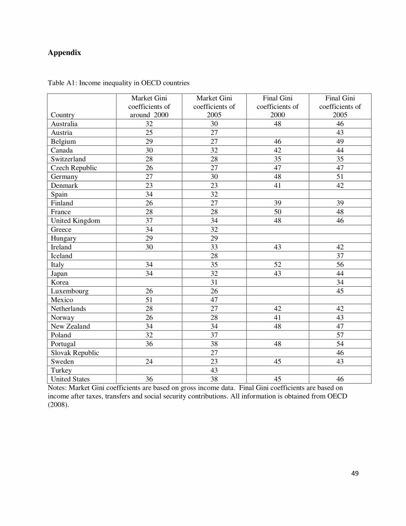
49

Appendix

Table A1: Income inequality in OECD countries

Country

Market Gini

coefficients of around 2000

Market Gini

coefficients of 2005

Final Gini

coefficients of 2000

Final Gini

coefficients of 2005

Australia 32 30 48 46

Austria 25 27 43

Belgium 29 27 46 49

Canada 30 32 42 44

Switzerland 28 28 35 35

Czech Republic 26 27 47 47

Germany 27 30 48 51

Denmark 23 23 41 42

Spain 34 32

Finland 26 27 39 39

France 28 28 50 48

United Kingdom 37 34 48 46

Greece 34 32

Hungary 29 29

Ireland 30 33 43 42

Iceland 28 37

Italy 34 35 52 56

Japan 34 32 43 44

Korea 31 34

Luxembourg 26 26 45

Mexico 51 47

Netherlands 28 27 42 42

Norway 26 28 41 43

New Zealand 34 34 48 47

Poland 32 37 57

Portugal 36 38 48 54

Slovak Republic 27 46

Sweden 24 23 45 43

Turkey 43

United States 36 38 45 46

Notes: Market Gini coefficients are based on gross income data. Final Gini coefficients are based on

income after taxes, transfers and social security contributions. All information is obtained from OECD

(2008).

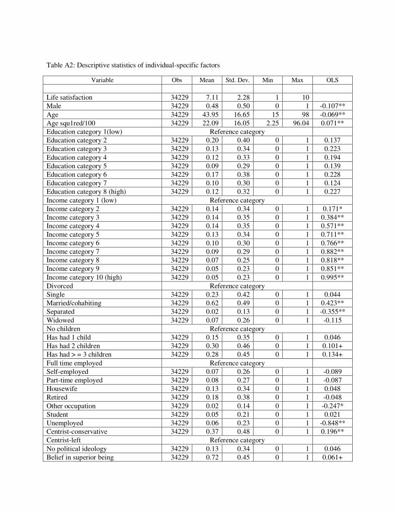
Table A2: Descriptive statistics of individual-specific factors

Variable Obs Mean Std. Dev. Min Max OLS

Life satisfaction 34229 7.11 2.28 1 10

Male 34229 0.48 0.50 0 1 -0.107**

Age 34229 43.95 16.65 15 98 -0.069**

Age squ1red/100 34229 22.09 16.05 2.25 96.04 0.071**

Education category 1(low) Reference category

Education category 2 34229 0.20 0.40 0 1 0.137

Education category 3 34229 0.13 0.34 0 1 0.223

Education category 4 34229 0.12 0.33 0 1 0.194

Education category 5 34229 0.09 0.29 0 1 0.139

Education category 6 34229 0.17 0.38 0 1 0.228

Education category 7 34229 0.10 0.30 0 1 0.124

Education category 8 (high) 34229 0.12 0.32 0 1 0.227

Income category 1 (low) Reference category

Income category 2 34229 0.14 0.34 0 1 0.171*

Income category 3 34229 0.14 0.35 0 1 0.384**

Income category 4 34229 0.14 0.35 0 1 0.571**

Income category 5 34229 0.13 0.34 0 1 0.711**

Income category 6 34229 0.10 0.30 0 1 0.766**

Income category 7 34229 0.09 0.29 0 1 0.882**

Income category 8 34229 0.07 0.25 0 1 0.818**

Income category 9 34229 0.05 0.23 0 1 0.851**

Income category 10 (high) 34229 0.05 0.23 0 1 0.995**

Divorced Reference category

Single 34229 0.23 0.42 0 1 0.044

Married/cohabiting 34229 0.62 0.49 0 1 0.423**

Separated 34229 0.02 0.13 0 1 -0.355**

Widowed 34229 0.07 0.26 0 1 -0.115

No children Reference category

Has had 1 child 34229 0.15 0.35 0 1 0.046

Has had 2 children 34229 0.30 0.46 0 1 0.101+

Has had > = 3 children 34229 0.28 0.45 0 1 0.134+

Full time employed Reference category

Self-employed 34229 0.07 0.26 0 1 -0.089

Part-time employed 34229 0.08 0.27 0 1 -0.087

Housewife 34229 0.13 0.34 0 1 0.048

Retired 34229 0.18 0.38 0 1 -0.048

Other occupation 34229 0.02 0.14 0 1 -0.247*

Student 34229 0.05 0.21 0 1 0.021

Unemployed 34229 0.06 0.23 0 1 -0.848**

Centrist-conservative 34229 0.37 0.48 0 1 0.196**

Centrist-left Reference category

No political ideology 34229 0.13 0.34 0 1 0.046

Belief in superior being 34229 0.72 0.45 0 1 0.061+

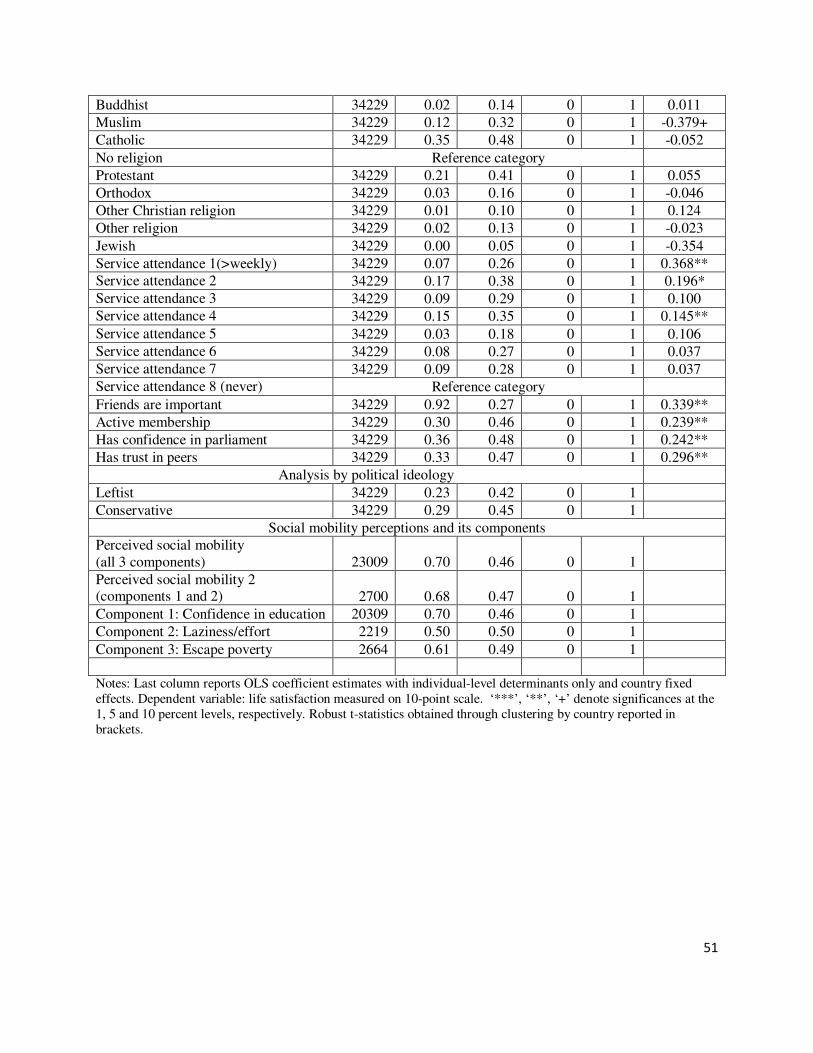
51

Buddhist 34229 0.02 0.14 0 1 0.011

Muslim 34229 0.12 0.32 0 1 -0.379+

Catholic 34229 0.35 0.48 0 1 -0.052

No religion Reference category

Protestant 34229 0.21 0.41 0 1 0.055

Orthodox 34229 0.03 0.16 0 1 -0.046

Other Christian religion 34229 0.01 0.10 0 1 0.124

Other religion 34229 0.02 0.13 0 1 -0.023

Jewish 34229 0.00 0.05 0 1 -0.354

Service attendance 1(>weekly) 34229 0.07 0.26 0 1 0.368**

Service attendance 2 34229 0.17 0.38 0 1 0.196*

Service attendance 3 34229 0.09 0.29 0 1 0.100

Service attendance 4 34229 0.15 0.35 0 1 0.145**

Service attendance 5 34229 0.03 0.18 0 1 0.106

Service attendance 6 34229 0.08 0.27 0 1 0.037

Service attendance 7 34229 0.09 0.28 0 1 0.037

Service attendance 8 (never) Reference category

Friends are important 34229 0.92 0.27 0 1 0.339**

Active membership 34229 0.30 0.46 0 1 0.239**

Has confidence in parliament 34229 0.36 0.48 0 1 0.242**

Has trust in peers 34229 0.33 0.47 0 1 0.296**

Analysis by political ideology

Leftist 34229 0.23 0.42 0 1

Conservative 34229 0.29 0.45 0 1

Social mobility perceptions and its components

Perceived social mobility

(all 3 components) 23009 0.70 0.46 0 1

Perceived social mobility 2 (components 1 and 2) 2700 0.68 0.47 0 1

Component 1: Confidence in education 20309 0.70 0.46 0 1

Component 2: Laziness/effort 2219 0.50 0.50 0 1

Component 3: Escape poverty 2664 0.61 0.49 0 1

Notes: Last column reports OLS coefficient estimates with individual-level determinants only and country fixed

effects. Dependent variable: life satisfaction measured on 10-point scale. ‘***’, ‘**’, ‘+’ denote significances at the

1, 5 and 10 percent levels, respectively. Robust t-statistics obtained through clustering by country reported in

brackets.

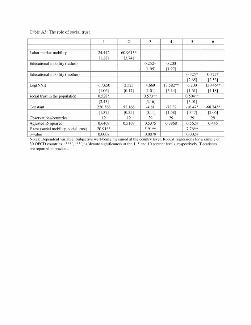
Table A3: The role of social trust

1 2 3 4 5 6

Labor market mobility 24.442 60.961**

[1.28] [3.74]

Educational mobility (father) 0.252+ 0.200

[1.95] [1.27]

Educational mobility (mother) 0.325* 0.327*

[2.65] [2.53]

Log(NNI) -17.650 2.525 4.669 13.582** 6.200 13.446**

[1.06] [0.17] [1.01] [3.14] [1.61] [4.18]

social trust in the population 0.528* 0.573** 0.504**

[2.43] [3.16] [3.01]

Constant 220.586 52.166 -4.81 -72.32 -16.475 -68.743*

[1.37] [0.35] [0.11] [1.58] [0.47] [2.06]

Observations/countries 12 12 29 29 29 29

Adjusted R-squared 0.6469 0.5169 0.5375 0.3868 0.5624 0.446

F-test (social mobility, social trust) 20.91** 5.91** 7.76**

p-value 0.0007 0.0079 0.0024

Notes: Dependent variable: Subjective well-being measured at the country level. Robust regressions for a sample of

30 OECD countries. ‘***’, ‘**’, ‘+’denote significances at the 1, 5 and 10 percent levels, respectively. T-statistics

are reported in brackets.

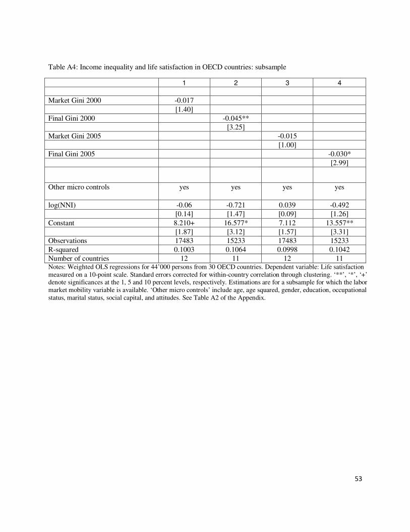
53

Table A4: Income inequality and life satisfaction in OECD countries: subsample

1 2 3 4

Market Gini 2000 -0.017

[1.40]

Final Gini 2000 -0.045**

[3.25]

Market Gini 2005 -0.015

[1.00]

Final Gini 2005 -0.030*

[2.99]

Other micro controls

yes

yes yes yes

log(NNI) -0.06 -0.721 0.039 -0.492

[0.14] [1.47] [0.09] [1.26]

Constant 8.210+ 16.577* 7.112 13.557**

[1.87] [3.12] [1.57] [3.31]

Observations 17483 15233 17483 15233

R-squared 0.1003 0.1064 0.0998 0.1042

Number of countries 12 11 12 11 Notes: Weighted OLS regressions for 44’000 persons from 30 OECD countries. Dependent variable: Life satisfaction

measured on a 10-point scale. Standard errors corrected for within-country correlation through clustering. ‘**’, ‘*’, ‘+’ denote significances at the 1, 5 and 10 percent levels, respectively. Estimations are for a subsample for which the labor

market mobility variable is available. ‘Other micro controls’ include age, age squared, gender, education, occupational

status, marital status, social capital, and attitudes. See Table A2 of the Appendix.

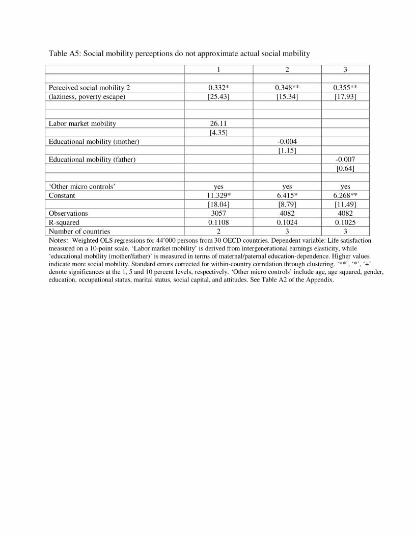
Table A5: Social mobility perceptions do not approximate actual social mobility

1 2 3

Perceived social mobility 2 0.332* 0.348** 0.355**

(laziness, poverty escape) [25.43] [15.34] [17.93]

Labor market mobility 26.11

[4.35]

Educational mobility (mother) -0.004

[1.15]

Educational mobility (father) -0.007

[0.64]

‘Other micro controls’ yes yes yes

Constant 11.329* 6.415* 6.268**

[18.04] [8.79] [11.49]

Observations 3057 4082 4082

R-squared 0.1108 0.1024 0.1025

Number of countries 2 3 3

Notes: Weighted OLS regressions for 44’000 persons from 30 OECD countries. Dependent variable: Life satisfaction

measured on a 10-point scale. ‘Labor market mobility’ is derived from intergenerational earnings elasticity, while

‘educational mobility (mother/father)’ is measured in terms of maternal/paternal education-dependence. Higher values

indicate more social mobility. Standard errors corrected for within-country correlation through clustering. ‘**’, ‘*’, ‘+’

denote significances at the 1, 5 and 10 percent levels, respectively. ‘Other micro controls’ include age, age squared, gender,

education, occupational status, marital status, social capital, and attitudes. See Table A2 of the Appendix.

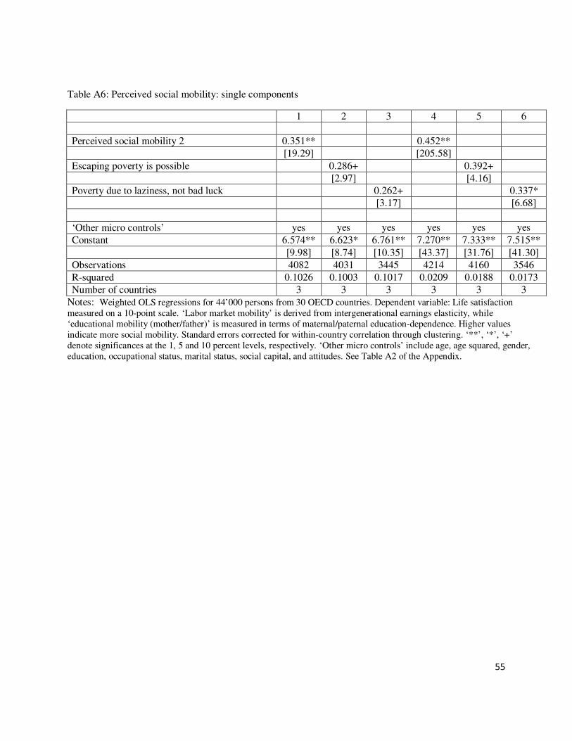
55

Table A6: Perceived social mobility: single components

1 2 3 4 5 6

Perceived social mobility 2 0.351** 0.452**

[19.29] [205.58]

Escaping poverty is possible 0.286+ 0.392+

[2.97] [4.16]

Poverty due to laziness, not bad luck 0.262+ 0.337*

[3.17] [6.68]

‘Other micro controls’ yes yes yes yes yes yes

Constant 6.574** 6.623* 6.761** 7.270** 7.333** 7.515**

[9.98] [8.74] [10.35] [43.37] [31.76] [41.30]

Observations 4082 4031 3445 4214 4160 3546

R-squared 0.1026 0.1003 0.1017 0.0209 0.0188 0.0173

Number of countries 3 3 3 3 3 3

Notes: Weighted OLS regressions for 44’000 persons from 30 OECD countries. Dependent variable: Life satisfaction

measured on a 10-point scale. ‘Labor market mobility’ is derived from intergenerational earnings elasticity, while

‘educational mobility (mother/father)’ is measured in terms of maternal/paternal education-dependence. Higher values

indicate more social mobility. Standard errors corrected for within-country correlation through clustering. ‘**’, ‘*’, ‘+’

denote significances at the 1, 5 and 10 percent levels, respectively. ‘Other micro controls’ include age, age squared, gender,

education, occupational status, marital status, social capital, and attitudes. See Table A2 of the Appendix.

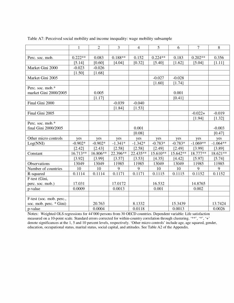
Table A7: Perceived social mobility and income inequality: wage mobility subsample

1 2 3 4 5 6 7 8

Perc. soc. mob. 0.222** 0.083 0.188** 0.152 0.224** 0.183 0.202** 0.356

[5.14] [0.60] [4.04] [0.32] [5.40] [1.62] [5.04] [1.11]

Market Gini 2000 -0.023 -0.026

[1.50] [1.68]

Market Gini 2005 -0.027 -0.028

[1.60] [1.74]

Perc. soc. mob.*

market Gini 2000/2005 0.005 0.001

[1.17] [0.41]

Final Gini 2000 -0.039 -0.040

[1.84] [1.53]

Final Gini 2005 -0.022+ -0.019

[1.94] [1.32]

Perc. soc. mob.*

final Gini 2000/2005 0.001 -0.003

[0.08] [0.47]

Other micro controls yes yes yes yes yes yes yes yes

Log(NNI) -0.902* -0.902* -1.341* -1.342* -0.783* -0.783* -1.069** -1.064**

[2.42] [2.43] [2.58] [2.58] [2.49] [2.49] [3.99] [3.89]

Constant 16.713** 16.806** 22.396** 22.435** 15.610** 15.642** 18.777** 18.621**

[3.92] [3.99] [3.57] [3.53] [4.35] [4.42] [5.97] [5.74]

Observations 13049 13049 11985 11985 13049 13049 11985 11985

Number of countries 10 10 9 9 10 10 9 9

R-squared 0.1114 0.1114 0.1171 0.1171 0.1115 0.1115 0.1152 0.1152

F-test (Gini,

perc. soc. mob.) 17.031 17.0172 16.532 14.8765

p-value 0.0009 0.0013 0.001 0.002

F-test (soc. mob. perc.,

soc. mob. perc. * Gini) 20.763 8.1332 15.3439 13.7424

p-value 0.0004 0.0118 0.0013 0.0026

Notes: Weighted OLS regressions for 44’000 persons from 30 OECD countries. Dependent variable: Life satisfaction

measured on a 10-point scale. Standard errors corrected for within-country correlation through clustering. ‘**’, ‘*’, ‘+’

denote significances at the 1, 5 and 10 percent levels, respectively. ‘Other micro controls’ include age, age squared, gender,

education, occupational status, marital status, social capital, and attitudes. See Table A2 of the Appendix.

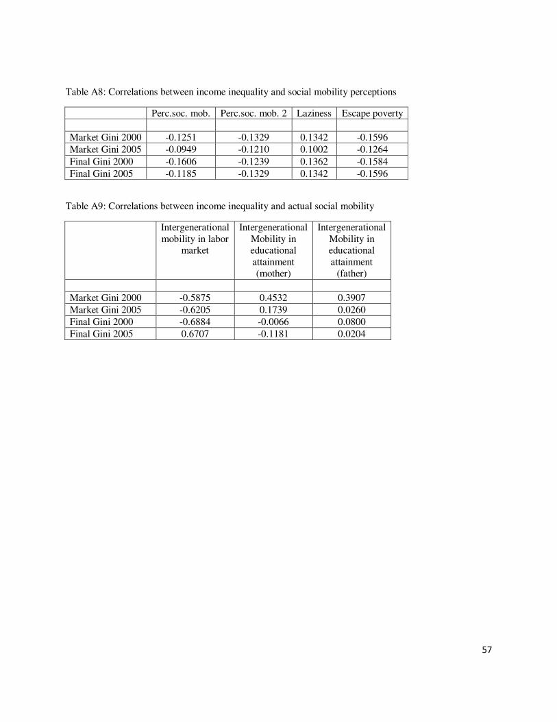
57

Table A8: Correlations between income inequality and social mobility perceptions

Perc.soc. mob. Perc.soc. mob. 2 Laziness Escape poverty

Market Gini 2000 -0.1251 -0.1329 0.1342 -0.1596

Market Gini 2005 -0.0949 -0.1210 0.1002 -0.1264

Final Gini 2000 -0.1606 -0.1239 0.1362 -0.1584

Final Gini 2005 -0.1185 -0.1329 0.1342 -0.1596

Table A9: Correlations between income inequality and actual social mobility

Intergenerational

mobility in labor market

Intergenerational

Mobility in educational

attainment

(mother)

Intergenerational

Mobility in educational

attainment

(father)

Market Gini 2000 -0.5875 0.4532 0.3907

Market Gini 2005 -0.6205 0.1739 0.0260

Final Gini 2000 -0.6884 -0.0066 0.0800

Final Gini 2005 0.6707 -0.1181 0.0204

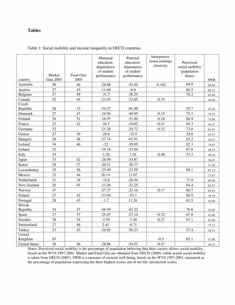
Tables

Table 1: Social mobility and income inequality in OECD countries

country

Market

Gini 2005

Final Gini

2005

Maternal

education-

dependence

of student

performance

Paternal

education-

dependence

of student

performance

Intergenera-

tional earnings

elasticity Perceived

social mobility

(population

share) SWB

Australia 30 46 -28.88 -35.44 -0.162 69.9 60.84

Austria 27 43 -11.69 -6.6 86.5 69.13

Belgium 27 49 -31.7 -28.29 78.2 62.46

Canada 32 44 -21.03 -23.05 -0.19 66.60

Czech

Republic 28 35 -54.27 -61.98 55.7 47.42

Denmark 27 47 -24.94 -40.95 -0.15 75.1 76.75

Finland 30 51 -16.97 -21.09 -0.18 88.9 72.68

France 23 42 -16.5 -19.02 -0.41 69.3 44.27

Germany 32 -21.28 -29.72 -0.32 73.8 61.63

Greece 27 39 -20.6 -15.9 29.0 41.57

Hungary 28 48 -57.74 -63.91 63.2 26.27

Iceland 34 46 -22 -20.05 82.3 74.43

Ireland 32 -19.18 -23.84 87.8 69.74

Italy 29 -1.28 3.26 -0.48 53.2 49.24

Japan 33 42 -28.49 -33.87 36.47

Korea 28 37 -20.31 -30.77 31.20

Luxembourg 35 56 -25.49 -23.59 68.1 65.75

Mexico 32 44 20.14 11.07 71.67

Netherlands 31 34 -32.6 -28.56 71.9 69.48

New Zealand 26 45 -13.26 -32.25 64.4 63.57

Norway 47 -27.37 -23.16 -0.17 80.7 63.93

Poland 27 42 -53.94 -55.1 80.9 38.79

Portugal 28 43 -1.7 11.26 61.5 41.04

Slovak

Republic 34 47 -48.59 -62.22 76.6 30.05

Spain 37 57 -25.07 -27.14 -0.32 67.8 42.80

Sweden 38 54 -2.59 -2.48 -0.27 67.1 62.96

Switzerland 27 46 2.41 -8.71 75.12

Turkey 23 43 -34.85 -50.23 57.4 28.52

United

Kingdom 43 -0.5 65.1 57.08

United States 38 46 -28.86 -34.53 -0.47 46.92

Notes: Perceived social mobility is the percentage of population believing that their society allows social mobility,

based on the WVS 1997-2001. Market and Final Gini are obtained from OECD (2008), while actual social mobility

is taken from OECD (2007). SWB is a measure of societal well-being, based on the WVS 1997-2001, measured as

the percentage of population expressing the three highest scores out of ten life satisfaction scores.

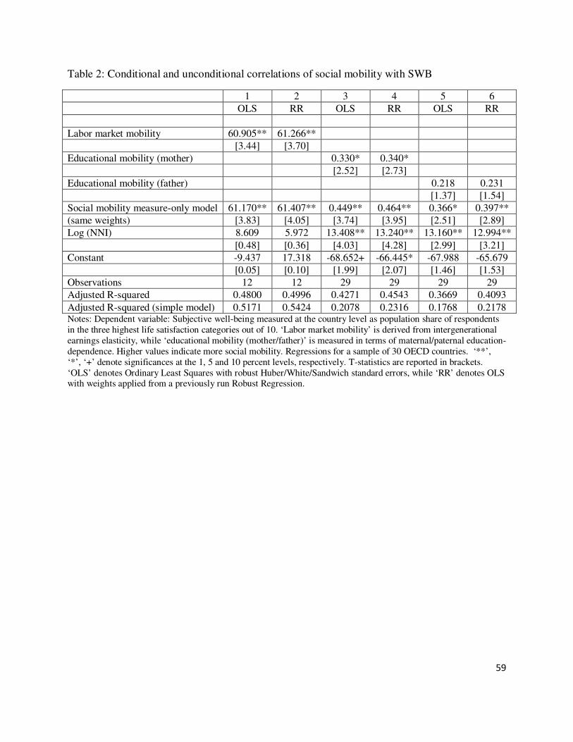
59

Table 2: Conditional and unconditional correlations of social mobility with SWB

1 2 3 4 5 6

OLS RR OLS RR OLS RR

Labor market mobility 60.905** 61.266**

[3.44] [3.70]

Educational mobility (mother) 0.330* 0.340*

[2.52] [2.73]

Educational mobility (father) 0.218 0.231

[1.37] [1.54]

Social mobility measure-only model 61.170** 61.407** 0.449** 0.464** 0.366* 0.397**

(same weights) [3.83] [4.05] [3.74] [3.95] [2.51] [2.89]

Log (NNI) 8.609 5.972 13.408** 13.240** 13.160** 12.994**

[0.48] [0.36] [4.03] [4.28] [2.99] [3.21]

Constant -9.437 17.318 -68.652+ -66.445* -67.988 -65.679

[0.05] [0.10] [1.99] [2.07] [1.46] [1.53]

Observations 12 12 29 29 29 29

Adjusted R-squared 0.4800 0.4996 0.4271 0.4543 0.3669 0.4093

Adjusted R-squared (simple model) 0.5171 0.5424 0.2078 0.2316 0.1768 0.2178 Notes: Dependent variable: Subjective well-being measured at the country level as population share of respondents

in the three highest life satisfaction categories out of 10. ‘Labor market mobility’ is derived from intergenerational

earnings elasticity, while ‘educational mobility (mother/father)’ is measured in terms of maternal/paternal education-

dependence. Higher values indicate more social mobility. Regressions for a sample of 30 OECD countries. ‘**’,

‘*’, ‘+’ denote significances at the 1, 5 and 10 percent levels, respectively. T-statistics are reported in brackets.

‘OLS’ denotes Ordinary Least Squares with robust Huber/White/Sandwich standard errors, while ‘RR’ denotes OLS with weights applied from a previously run Robust Regression.

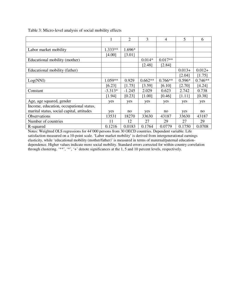
Table 3: Micro-level analysis of social mobility effects

1 2 3 4 5 6

Labor market mobility 1.333** 1.696*

[4.00] [3.01]

Educational mobility (mother) 0.014* 0.017**

[2.48] [2.84]

Educational mobility (father) 0.013+ 0.012+

[2.04] [1.75]

Log(NNI) 1.059** 0.929 0.662** 0.766** 0.596* 0.746**

[6.23] [1.75] [3.59] [6.10] [2.70] [4.24]

Constant -3.313* -1.245 2.029 0.623 2.742 0.738

[1.94] [0.23] [1.00] [0.46] [1.11] [0.38]

Age, age squared, gender yes yes yes yes yes yes

Income, education, occupational status,

marital status, social capital, attitudes yes no yes no yes no

Observations 13531 18270 33630 43187 33630 43187

Number of countries 11 12 27 29 27 29

R-squared 0.1216 0.0183 0.1764 0.0779 0.1750 0.0708 Notes: Weighted OLS regressions for 44’000 persons from 30 OECD countries. Dependent variable: Life

satisfaction measured on a 10-point scale. ‘Labor market mobility’ is derived from intergenerational earnings

elasticity, while ‘educational mobility (mother/father)’ is measured in terms of maternal/paternal education-

dependence. Higher values indicate more social mobility. Standard errors corrected for within-country correlation

through clustering. ‘**’, ‘*’, ‘+’ denote significances at the 1, 5 and 10 percent levels, respectively.

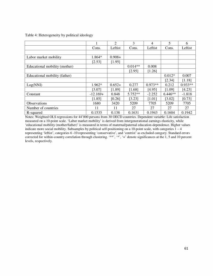
61

Table 4: Heterogeneity by political ideology

1 2 3 4 5 6

Cons. Leftist Cons. Leftist Cons. Leftist

Labor market mobility 1.864* 0.908+

[2.53] [1.95]

Educational mobility (mother) 0.014** 0.008

[2.95] [1.26]

Educational mobility (father) 0.012* 0.007

[2.34] [1.18]

Log(NNI) 1.962* 0.652+ 0.277 0.973** 0.212 0.933**

[3.07] [1.89] [1.68] [4.95] [1.09] [4.23]

Constant -12.169+ 0.848 5.752** -2.252 6.446** -1.818

[1.85] [0.26] [3.23] [1.01] [3.02] [0.73]

Observations 1680 3420 5209 7705 5209 7705

Number of countries 11 11 27 27 27 27

R-squared 0.1535 0.138 0.1631 0.1943 0.1604 0.1942 Notes: Weighted OLS regressions for 44’000 persons from 30 OECD countries. Dependent variable: Life satisfaction

measured on a 10-point scale. ‘Labor market mobility’ is derived from intergenerational earnings elasticity, while

‘educational mobility (mother/father)’ is measured in terms of maternal/paternal education-dependence. Higher values

indicate more social mobility. Subsamples by political self-positioning on a 10-point scale, with categories 1 – 4

representing ‘leftist’, categories 6 -10 representing ‘conservative’, and ‘centrist’ as excluded category. Standard errors

corrected for within-country correlation through clustering. ‘**’, ‘*’, ‘+’ denote significances at the 1, 5 and 10 percent

levels, respectively.

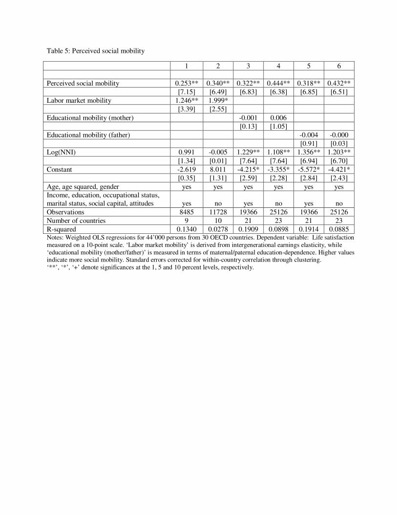
Table 5: Perceived social mobility

1 2 3 4 5 6

Perceived social mobility 0.253** 0.340** 0.322** 0.444** 0.318** 0.432**

[7.15] [6.49] [6.83] [6.38] [6.85] [6.51]

Labor market mobility 1.246** 1.999*

[3.39] [2.55]

Educational mobility (mother) -0.001 0.006

[0.13] [1.05]

Educational mobility (father) -0.004 -0.000

[0.91] [0.03]

Log(NNI) 0.991 -0.005 1.229** 1.108** 1.356** 1.203**

[1.34] [0.01] [7.64] [7.64] [6.94] [6.70]

Constant -2.619 8.011 -4.215* -3.355* -5.572* -4.421*

[0.35] [1.31] [2.59] [2.28] [2.84] [2.43]

Age, age squared, gender yes yes yes yes yes yes

Income, education, occupational status,

marital status, social capital, attitudes yes no yes no yes no

Observations 8485 11728 19366 25126 19366 25126

Number of countries 9 10 21 23 21 23

R-squared 0.1340 0.0278 0.1909 0.0898 0.1914 0.0885 Notes: Weighted OLS regressions for 44’000 persons from 30 OECD countries. Dependent variable: Life satisfaction

measured on a 10-point scale. ‘Labor market mobility’ is derived from intergenerational earnings elasticity, while

‘educational mobility (mother/father)’ is measured in terms of maternal/paternal education-dependence. Higher values indicate more social mobility. Standard errors corrected for within-country correlation through clustering.

‘**’, ‘*’, ‘+’ denote significances at the 1, 5 and 10 percent levels, respectively.

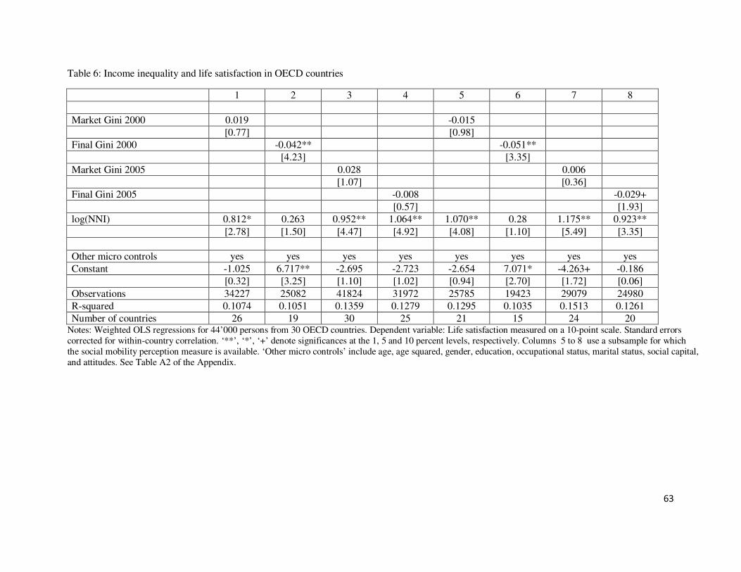
63

Table 6: Income inequality and life satisfaction in OECD countries

1 2 3 4 5 6 7 8

Market Gini 2000 0.019 -0.015

[0.77] [0.98]

Final Gini 2000 -0.042** -0.051**

[4.23] [3.35]

Market Gini 2005 0.028 0.006

[1.07] [0.36]

Final Gini 2005 -0.008 -0.029+

[0.57] [1.93]

log(NNI) 0.812* 0.263 0.952** 1.064** 1.070** 0.28 1.175** 0.923**

[2.78] [1.50] [4.47] [4.92] [4.08] [1.10] [5.49] [3.35]

Other micro controls yes yes yes yes yes yes yes yes

Constant -1.025 6.717** -2.695 -2.723 -2.654 7.071* -4.263+ -0.186

[0.32] [3.25] [1.10] [1.02] [0.94] [2.70] [1.72] [0.06]

Observations 34227 25082 41824 31972 25785 19423 29079 24980

R-squared 0.1074 0.1051 0.1359 0.1279 0.1295 0.1035 0.1513 0.1261

Number of countries 26 19 30 25 21 15 24 20 Notes: Weighted OLS regressions for 44’000 persons from 30 OECD countries. Dependent variable: Life satisfaction measured on a 10-point scale. Standard errors

corrected for within-country correlation. ‘**’, ‘*’, ‘+’ denote significances at the 1, 5 and 10 percent levels, respectively. Columns 5 to 8 use a subsample for which

the social mobility perception measure is available. ‘Other micro controls’ include age, age squared, gender, education, occupational status, marital status, social capital,

and attitudes. See Table A2 of the Appendix.

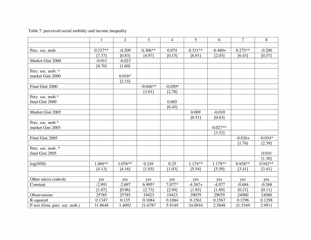
Table 7: perceived social mobility and income inequality

1 2 3 4 5 6 7 8

Perc. soc. mob. 0.337** -0.209 0.306** 0.074 0.331** -0.480+ 0.275** -0.200

[7.37] [0.83] [4.97] [0.15] [6.91] [2.03] [6.43] [0.57]

Market Gini 2000 -0.011 -0.023

[0.76] [1.60]

Perc. soc. mob. * market Gini 2000 0.018*

[2.15]

Final Gini 2000 -0.046** -0.050*

[3.01] [2.78]

Perc. soc. mob.* final Gini 2000 0.005

[0.45]

Market Gini 2005 0.009 -0.010

[0.51] [0.63]

Perc. soc. mob.*

market Gini 2005 0.027**

[3.52]

Final Gini 2005 -0.026+ -0.034*

[1.76] [2.39]

Perc. soc. mob. *

final Gini 2005 0.010

[1.30]

log(NNI) 1.069** 1.076** 0.249 0.25 1.174** 1.179** 0.938** 0.942**

[4.13] [4.16] [1.03] [1.03] [5.54] [5.59] [3.41] [3.41]

Other micro controls yes yes yes yes yes yes yes yes

Constant -2.991 -2.697 6.905* 7.077* -4.567+ -4.077 -0.684 -0.368

[1.07] [0.96] [2.73] [2.94] [1.85] [1.69] [0.21] [0.11]

Observations 25785 25785 19423 19423 29079 29079 24980 24980

R-squared 0.1347 0.135 0.1084 0.1084 0.1561 0.1567 0.1296 0.1298

F-test (Gini, perc. soc. mob.) 31.8648 1.4092 21.6787 5.9149 24.0916 2.5848 21.5169 2.9911

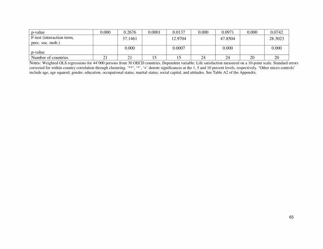
65

p-value 0.000 0.2676 0.0001 0.0137 0.000 0.0971 0.000 0.0742

F-test (interaction term,

perc. soc. mob.) 37.1461 12.9704 47.8504 28.3023

p-value 0.000 0.0007 0.000 0.000

Number of countries 21 21 15 15 24 24 20 20

Notes: Weighted OLS regressions for 44’000 persons from 30 OECD countries. Dependent variable: Life satisfaction measured on a 10-point scale. Standard errors

corrected for within-country correlation through clustering. ‘**’, ‘*’, ‘+’ denote significances at the 1, 5 and 10 percent levels, respectively. ‘Other micro controls’

include age, age squared, gender, education, occupational status, marital status, social capital, and attitudes. See Table A2 of the Appendix.

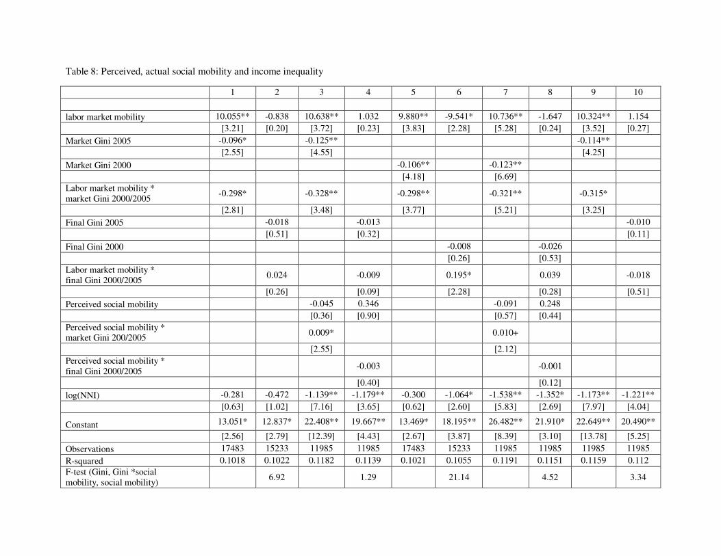
Table 8: Perceived, actual social mobility and income inequality

1 2 3 4 5 6 7 8 9 10

labor market mobility 10.055** -0.838 10.638** 1.032 9.880** -9.541* 10.736** -1.647 10.324** 1.154

[3.21] [0.20] [3.72] [0.23] [3.83] [2.28] [5.28] [0.24] [3.52] [0.27]

Market Gini 2005 -0.096* -0.125** -0.114**

[2.55] [4.55] [4.25]

Market Gini 2000 -0.106** -0.123**

[4.18] [6.69]

Labor market mobility *

market Gini 2000/2005 -0.298* -0.328** -0.298** -0.321** -0.315*

[2.81] [3.48] [3.77] [5.21] [3.25]

Final Gini 2005 -0.018 -0.013 -0.010

[0.51] [0.32] [0.11]

Final Gini 2000 -0.008 -0.026

[0.26] [0.53]

Labor market mobility *

final Gini 2000/2005 0.024 -0.009 0.195* 0.039 -0.018

[0.26] [0.09] [2.28] [0.28] [0.51]

Perceived social mobility -0.045 0.346 -0.091 0.248

[0.36] [0.90] [0.57] [0.44]

Perceived social mobility * market Gini 200/2005

0.009* 0.010+

[2.55] [2.12]

Perceived social mobility *

final Gini 2000/2005 -0.003 -0.001

[0.40] [0.12]

log(NNI) -0.281 -0.472 -1.139** -1.179** -0.300 -1.064* -1.538** -1.352* -1.173** -1.221**

[0.63] [1.02] [7.16] [3.65] [0.62] [2.60] [5.83] [2.69] [7.97] [4.04]

Constant 13.051* 12.837* 22.408** 19.667** 13.469* 18.195** 26.482** 21.910* 22.649** 20.490**

[2.56] [2.79] [12.39] [4.43] [2.67] [3.87] [8.39] [3.10] [13.78] [5.25]

Observations 17483 15233 11985 11985 17483 15233 11985 11985 11985 11985

R-squared 0.1018 0.1022 0.1182 0.1139 0.1021 0.1055 0.1191 0.1151 0.1159 0.112

F-test (Gini, Gini *social

mobility, social mobility) 6.92 1.29 21.14 4.52 3.34

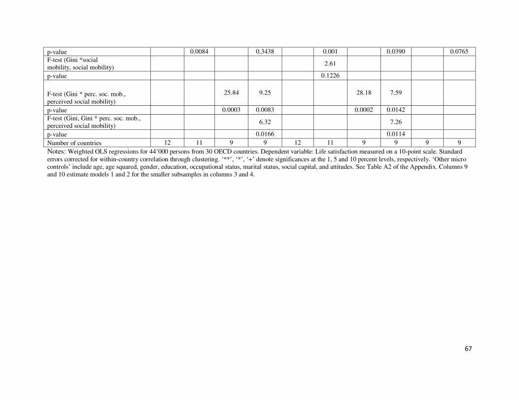
67

p-value 0.0084 0.3438 0.001 0.0390 0.0765

F-test (Gini *social

mobility, social mobility) 2.61

p-value 0.1226

F-test (Gini * perc. soc. mob.,

perceived social mobility)

25.84 9.25 28.18 7.59

p-value 0.0003 0.0083 0.0002 0.0142

F-test (Gini, Gini * perc. soc. mob.,

perceived social mobility) 6.32 7.26

p-value 0.0166 0.0114

Number of countries 12 11 9 9 12 11 9 9 9 9

Notes: Weighted OLS regressions for 44’000 persons from 30 OECD countries. Dependent variable: Life satisfaction measured on a 10-point scale. Standard

errors corrected for within-country correlation through clustering. ‘**’, ‘*’, ‘+’ denote significances at the 1, 5 and 10 percent levels, respectively. ‘Other micro

controls’ include age, age squared, gender, education, occupational status, marital status, social capital, and attitudes. See Table A2 of the Appendix. Columns 9

and 10 estimate models 1 and 2 for the smaller subsamples in columns 3 and 4.

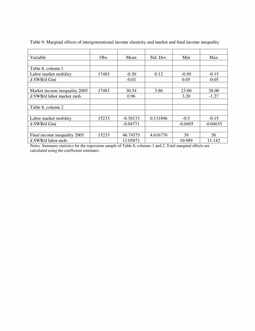
Table 9: Marginal effects of intergenerational income elasticity and market and final income inequality

Variable Obs. Mean Std. Dev. Min Max

Table 8, column 1

Labor market mobility 17483 -0.30 0.12 -0.50 -0.15

d SWB/d Gini -0.01 0.05 -0.05

Market income inequality 2005 17483 30.54 3.86 23.00 38.00

d SWB/d labor market mob. 0.96 3.20 -1.27

Table 8, column 2

Labor market mobility 15233 -0.30133 0.131896 -0.5 -0.15

d SWB/d Gini -0.04771 -0.0495 -0.04635

Final income inequality 2005 15233 46.74575 4.616776 39 56

d SWB/d labor.mob. 11.05871 10.989 11.142 Notes: Summary statistics for the regression sample of Table 8, columns 1 and 2. Total marginal effects are

calculated using the coefficient estimates.

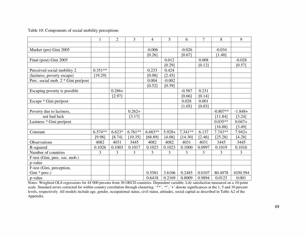
69

Table 10: Components of social mobility perceptions

1 2 3 4 5 6 7 8 9

Market (pre) Gini 2005 -0.006 -0.026 -0.034

[0.26] [0.67] [1.40]

Final (post) Gini 2005 0.012 0.008 -0.028

[0.29] [0.12] [0.57]

Perceived social mobility 2 0.351** 0.233 0.424

(laziness, poverty escape) [19.29] [0.98] [2.45]

Perc. social mob. 2 * Gini pre/post 0.004 -0.002

[0.52] [0.39]

Escaping poverty is possible 0.286+ -0.587 0.231

[2.97] [0.66] [0.14]

Escape * Gini pre/post 0.028 0.001

[1.05] [0.03]

Poverty due to laziness, 0.262+ -0.807** -1.848+

not bad luck [3.17] [11.84] [3.24]

Laziness * Gini pre/post 0.035** 0.047+

[16.88] [3.49]

Constant 6.574** 6.623* 6.761** 6.683** 5.928+ 7.341** 6.137 7.743** 7.942+

[9.98] [8.74] [10.35] [68.89] [4.08] [14.30] [2.46] [25.28] [4.28]

Observations 4082 4031 3445 4082 4082 4031 4031 3445 3445

R-squared 0.1026 0.1003 0.1017 0.1023 0.1023 0.1000 0.0997 0.1019 0.1016

Number of countries 3 3 3 3 3 3 3 3 3

F-test (Gini, perc. soc. mob.)

p-value

F-test (Gini, perception, Gini * perc.) 0.5581 3.6106 0.2485 0.0107 80.4978 1030.594

p-value 0.6418 0.2169 0.8009 0.9894 0.0123 0.001 Notes: Weighted OLS regressions for 44’000 persons from 30 OECD countries. Dependent variable: Life satisfaction measured on a 10-point

scale. Standard errors corrected for within-country correlation through clustering. ‘**’, ‘*’, ‘+’ denote significances at the 1, 5 and 10 percent

levels, respectively. All models include age, gender, occupational status, civil status, attitudes, social capital as described in Table A2 of the

Appendix.

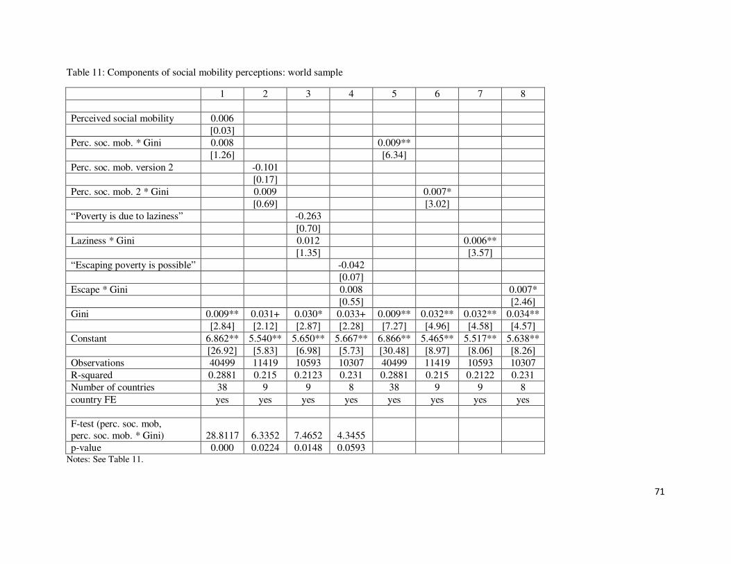
71

Table 11: Components of social mobility perceptions: world sample

1 2 3 4 5 6 7 8

Perceived social mobility 0.006

[0.03]

Perc. soc. mob. * Gini 0.008 0.009**

[1.26] [6.34]

Perc. soc. mob. version 2 -0.101

[0.17]

Perc. soc. mob. 2 * Gini 0.009 0.007*

[0.69] [3.02]

“Poverty is due to laziness” -0.263

[0.70]

Laziness * Gini 0.012 0.006**

[1.35] [3.57]

“Escaping poverty is possible” -0.042

[0.07]

Escape * Gini 0.008 0.007*

[0.55] [2.46]

Gini 0.009** 0.031+ 0.030* 0.033+ 0.009** 0.032** 0.032** 0.034**

[2.84] [2.12] [2.87] [2.28] [7.27] [4.96] [4.58] [4.57]

Constant 6.862** 5.540** 5.650** 5.667** 6.866** 5.465** 5.517** 5.638**

[26.92] [5.83] [6.98] [5.73] [30.48] [8.97] [8.06] [8.26]

Observations 40499 11419 10593 10307 40499 11419 10593 10307

R-squared 0.2881 0.215 0.2123 0.231 0.2881 0.215 0.2122 0.231

Number of countries 38 9 9 8 38 9 9 8

country FE yes yes yes yes yes yes yes yes

F-test (perc. soc. mob,

perc. soc. mob. * Gini) 28.8117 6.3352 7.4652 4.3455

p-value 0.000 0.0224 0.0148 0.0593 Notes: See Table 11.

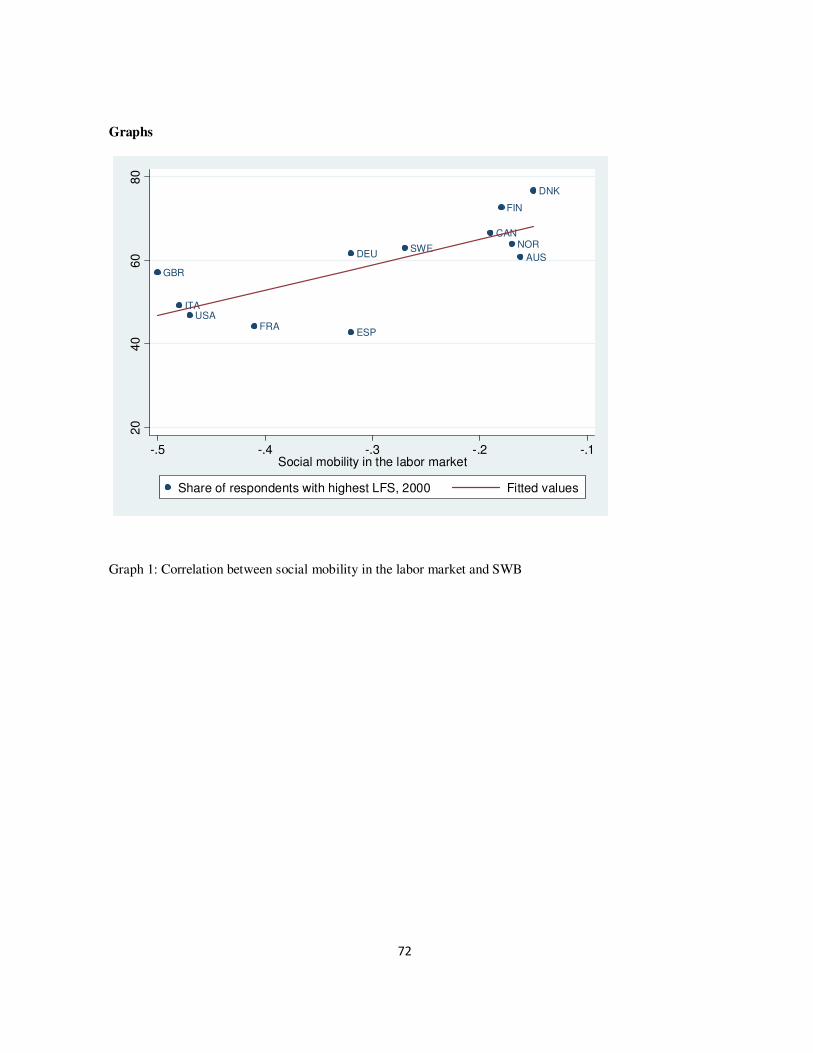
72

Graphs

AUS

CAN

DEU

DNK

ESP

FIN

FRA

GBR

ITA

NORSWE

USA

20

40

60

80

-.5 -.4 -.3 -.2 -.1Social mobility in the labor market

Share of respondents with highest LFS, 2000 Fitted values

Graph 1: Correlation between social mobility in the labor market and SWB

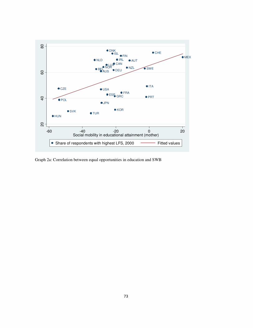
73

AUS

AUT

BEL

CAN

CHE

CZE

DEU

DNK

ESP

FIN

FRAGRC

HUN

IRL

ISL

ITA

JPN

KOR

LUX

MEXNLD

NOR NZL

POLPRT

SVK

SWE

TUR

USA

20

40

60

80

-60 -40 -20 0 20Social mobility in educational attainment (mother)

Share of respondents with highest LFS, 2000 Fitted values

Graph 2a: Correlation between equal opportunities in education and SWB

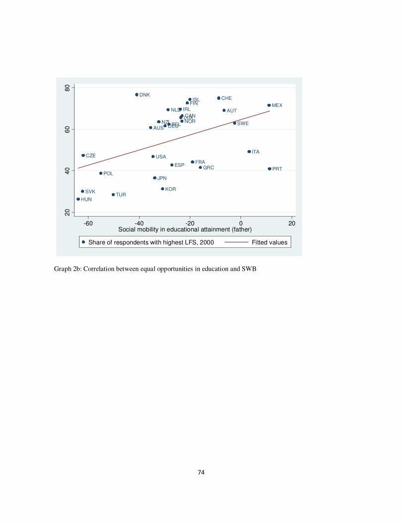
74

AUS

AUT

BEL

CAN

CHE

CZE

DEU

DNK

ESP

FIN

FRAGRC

HUN

IRL

ISL

ITA

JPN

KOR

LUX

MEXNLD

NORNZL

POLPRT

SVK

SWE

TUR

USA

20

40

60

80

-60 -40 -20 0 20Social mobility in educational attainment (father)

Share of respondents with highest LFS, 2000 Fitted values

Graph 2b: Correlation between equal opportunities in education and SWB

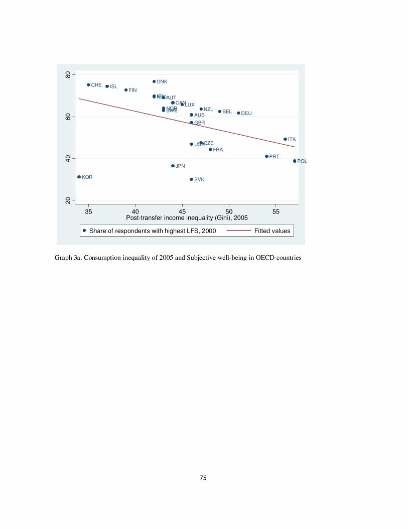
75

AUS

AUT

BEL

CAN

CHE

CZE

DEU

DNK

FIN

FRA

GBR

IRL

ISL

ITA

JPN

KOR

LUX

NLD

NOR NZL

POLPRT

SVK

SWE

USA

20

40

60

80

35 40 45 50 55Post-transfer income inequality (Gini), 2005

Share of respondents with highest LFS, 2000 Fitted values

Graph 3a: Consumption inequality of 2005 and Subjective well-being in OECD countries

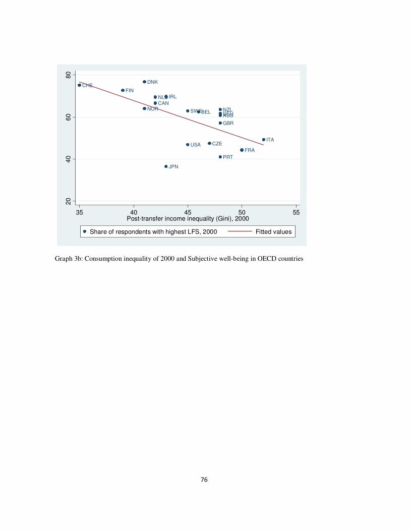
76

AUSBEL

CAN

CHE

CZE

DEU

DNK

FIN

FRA

GBR

IRL

ITA

JPN

NLD

NOR NZL

PRT

SWE

USA

20

40

60

80

35 40 45 50 55Post-transfer income inequality (Gini), 2000

Share of respondents with highest LFS, 2000 Fitted values

Graph 3b: Consumption inequality of 2000 and Subjective well-being in OECD countries

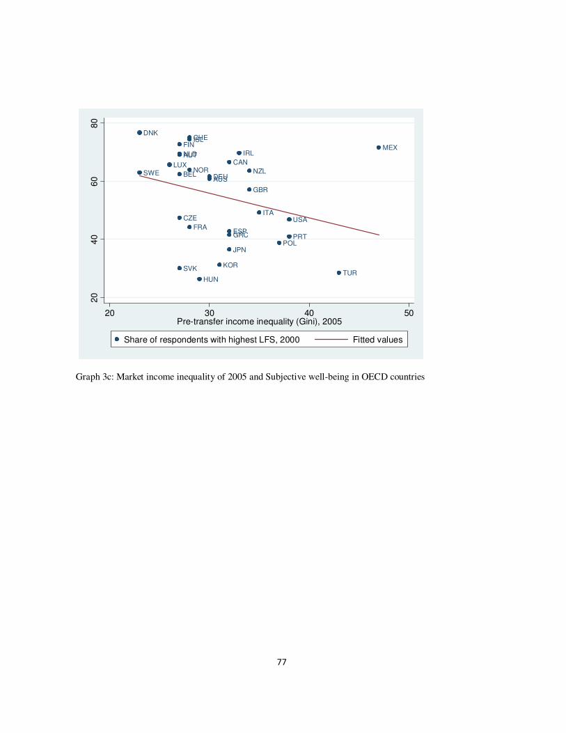
77

AUS

AUT

BEL

CAN

CHE

CZE

DEU

DNK

ESP

FIN

FRA

GBR

GRC

HUN

IRL

ISL

ITA

JPN

KOR

LUX

MEXNLD

NOR NZL

POLPRT

SVK

SWE

TUR

USA

20

40

60

80

20 30 40 50Pre-transfer income inequality (Gini), 2005

Share of respondents with highest LFS, 2000 Fitted values

Graph 3c: Market income inequality of 2005 and Subjective well-being in OECD countries

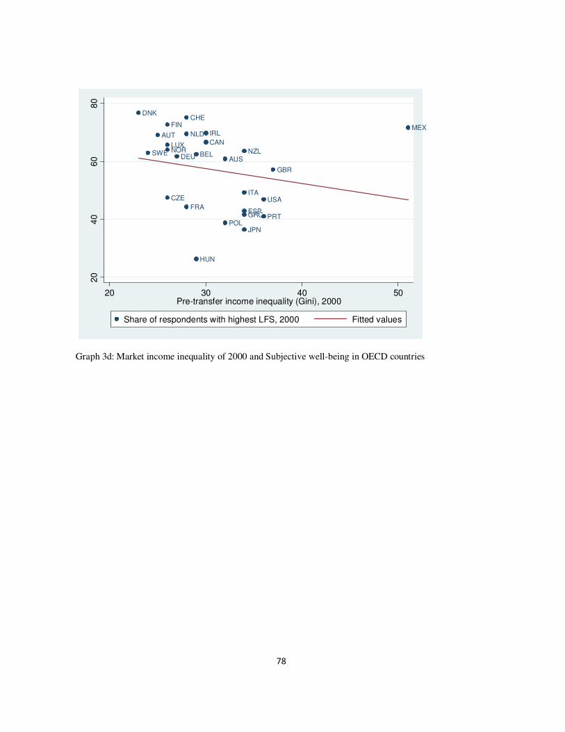
78

AUS

AUT

BEL

CAN

CHE

CZE

DEU

DNK

ESP

FIN

FRA

GBR

GRC

HUN

IRL

ITA

JPN

LUX

MEXNLD

NOR NZL

POLPRT

SWE

USA

20

40

60

80

20 30 40 50Pre-transfer income inequality (Gini), 2000

Share of respondents with highest LFS, 2000 Fitted values

Graph 3d: Market income inequality of 2000 and Subjective well-being in OECD countries