Groupe de Recherche en Économie et Développement International
Cahier de recherche / Working Paper 04-07
Macroeconomic Growth, Sectoral Quality of Growth and Poverty in Developing Countries : Measure and Application to Burkina Faso
Dorothée Boccanfuso
Tambi Samuel Kaboré
M AC R O E C O N O M I C G R OW T H , S E C T O R A L Q UA L I T Y O F G R OW T H A N D P OV E R T Y I N D E V E L O P I N G
C O U N T R I E S : M E A S U R E A N D A P P L I C A T I O N T O B U R K I N A FA S O
Dorothée BOCCANFUSO1, Tambi Samuel KABORE2
O c t o b e r 2 0 0 4
Abstract
Economic growth generally refers to GDP growth. The studies on the link between growth and poverty dynamic (Datt and Ravallion, 1992; Kakwani, 1997; Shorrocks, 1999) measure growth by mean household per capita expenditures. Furthermore, many countries experience at the same time economic growth and growing poverty. It is therefore important to establish a link between these two types of growth. This key link allows a formal shift from macroeconomic growth (GDP growth) to mean per capita household expenditure growth.
The purpose of this paper is to discuss the link between macroeconomic growth and mean per capita household expenditure growth with the evidence drawn from Burkina Faso data. The paper also analyzes the impact of sectoral growth on poverty using Shapley value-based decomposition approach. National Accounts consumption - which is smaller - gives greater poverty incidences for 1994 and 1998 compared to the incidence from the surveys’ consumption. An annual 3.99% increase in real per capita consumption based on the survey gives a 13.37% decrease in poverty incidence, while a 6.59% annual growth in GDP yields only 6.59% decrease in poverty incidence. Agricultural sector growth accounts for at least 80% of the decline in poverty incidence, gap and severity.
Key words: Growth, Poverty decomposition, Shapley Value, Burkina Faso
J E L :
1 Université de Sherbrooke, Département d’économique – Faculté d’administration ; Email : [email protected]. 2 CEDRES, UFR-SEG-Université de Ouagadougou, 01 BP 6693 Ouaga 01, Email : [email protected], [email protected].
Introduction ___________________________________________________________ 2
Introduction ___________________________________________________________ 2
1. literature Review ___________________________________________________ 4
2. Concepts and methods _______________________________________________ 6 2.1. Economic Growth and Growth of Mean Expenditure ______________________ 6 3-2 Sectoral Growth and Poverty Reduction _________________________________ 9
3. Data and sector characteristics _______________________________________ 11
4. Findings _________________________________________________________ 12 4.1. Relation between Consumption, GDP and Poverty ________________________ 12 4.2. Economic decomposition _____________________________________________ 16 4.3. Regional decomposition ______________________________________________ 19 4.4. Agricultural decomposition ___________________________________________ 20
5. Conclusion and economic policy implications ___________________________ 22
6. Bibliography______________________________________________________ 23
7. Appendix_________________________________________________________ 25 Table 1: FGT poverty measures and per capita average consumption in sectors in Burkina Faso (1994
and 1998). ______________________________________________________________________ 12 Table 2 : Evolution of macroeconomic data in Burkina Faso (94-98) __________________________ 13 Table 3: Relative Impacts of sectoral growth (Gk), redistribution (Dk), and change in population size
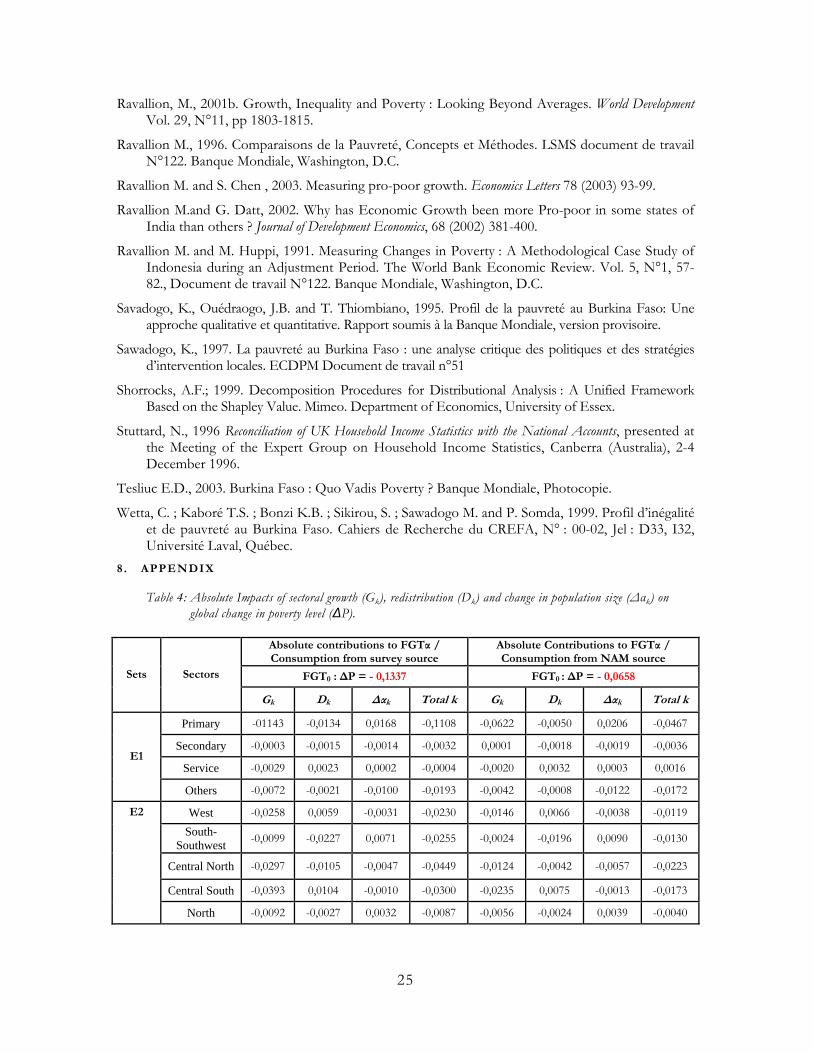
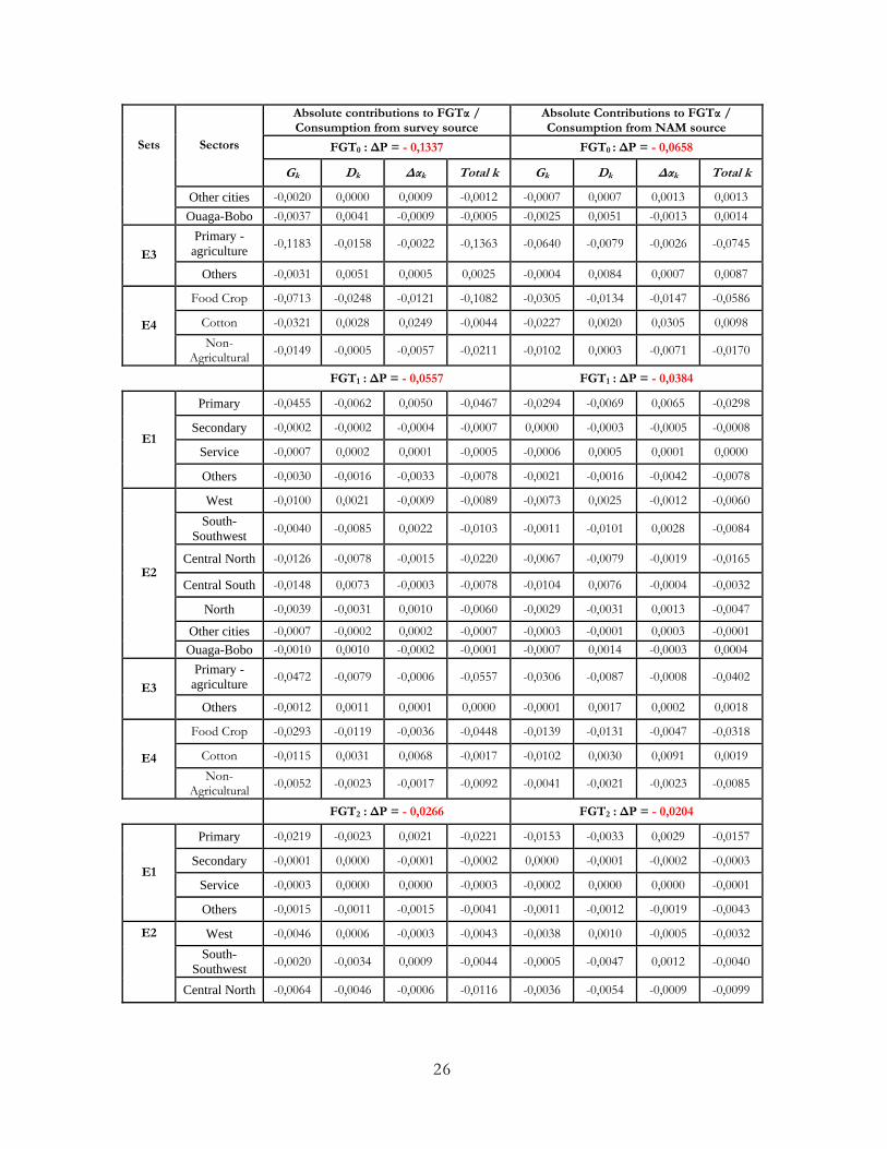
(∆αk) on global change in poverty level (∆P). _________________________________________ 16 Table 4: Absolute Impacts of sectoral growth (Gk), redistribution (Dk) and change in population size
(∆αk) on global change in poverty level (∆P). _________________________________________ 25
Figure 1: Comparative table of mean expenditure (�) and GDP growth: Burkina Faso 94-98.......... 14 Figure 2 : Implication for poverty analysis (FGT0 %) ............................................................................. 15 Figure 3 : Contributions of regional growth and redistribution to FGT0 variation.............................. 19 Figure 4: Contributions of agricultural growths and redistribution to FGT0 variation ...................... 20
2
INTRODUCTION
The Government of Burkina Faso’s efforts to promote the country’s development have been
dominated over the past fifteen years by the structural adjustment programs (SAP) adopted in 1991.
The impact of this policy package, combined with that of the devaluation of the CFA Franc (January
1994) resulted in a 5% annual increase in real GDP over the 1995-19983 period, compared to an
average 1.5% increase over the 1993-1995 period. According to the statistics institute (INSD, 2000),
increases of consumption (8.8%), investments (18.4%) and exports (12%) are largely responsible for
this growth.
Despite these positive macroeconomic achievements, poverty remains an important social
phenomenon, which has tended to increase during the same period. Poverty headcount ratio rose
from 44.5% in 1994 to 45.3% in 1998 and to 46.4% in 2003. These variations in poverty levels
contradict the growth effect, and when combined with stable inequality indices, the results appear to
be inconsistent with expectations. Inconsistency might be linked to the use of inappropriate methods
to evaluate poverty (Tesliuc, 2003). These previous poverty measures have been evaluated using
nominal per capita expenditures, as in official reports. Computing the same measures with real per capita
expenditures can mitigate conclusions on poverty trends (Boccanfuso and Kaboré, 2003).
Understanding the links between growth and poverty becomes a major challenge both in research and
policy debates. Recent literature came to the conclusion that the link between growth and poverty
reduction is not a systematic one, suggesting that growth is not a sufficient condition to reduce
poverty (Bigsten and Levin, 2000 ; de Janvry and Sadoulet, 2000 ; Ravallion and Datt, 2002 ; Bigsten
et al., 2002). Bourguignon (2003) tried to clarify the debate on development strategies focusing on
growth and income distribution by providing a rigorous framework for the analysis of the relationship
existing between the three vertices of the Poverty Growth Inequality (PGI) triangle.
Debate is ongoing in three areas. One of these areas questions the pro-poor nature of growth focused
on growth incidence on the poor (Dollar and Kraay, 2000; Ravallion and Chen, 2003) or on sectoral
growth (Fan et al., 2000; Ravallion and Datt, 2002). The second subject of debate is the data issue
(Ravallion, 2001a; Deaton, 2004). National Accounts (NAM) data and Household Survey (HS) data
do not give an identical picture of the same phenomenon due to conceptual and methodological
differences. These inconsistencies may have misleading implications for policy reforms and especially
for the poverty decomposition. The relevant literature has raised this problem but household surveys
are generally assumed to be more accurate and independent than national accounts, it (HS) seems to
3 This growth trend was maintained until 2002 despite a marginal decrease in 2000 (2.14%) (WAEMU Commission, December 2002)
2
be the source most commonly used. The third subject of debate centers on the relevance of the
methods used to capture poverty trends (Tesliuc, 2003). Some methodological issues like
“comparison of non-equivalent welfare measures”, “benchmark period”, and “quality of regional
price statistics” can change consumption-based poverty measures and subsequently poverty dynamics
in this context. This paper focuses on the first two points, notably data issues and sectoral growth
issues with an empirical application to Burkina Faso.
Ravallion (2001a) and Deaton (2004) underlined that recent applied work showed growing interest in
the link between NAM and HS data sources. Understanding the relationship between household
surveys and national accounts data and its implications for poverty analysis is a major challenge.
Economic growth generally refers to GDP growth, which reduces poverty (when distribution remains
constant). Since poverty is usually measured by household survey data, survey per capita expenditure
(PCE) growth is used to calculate the impact of growth on poverty dynamics instead of GDP
growth. This paper attempts to shed some light on this controversy (Ravallion, 2003; Deaton, 2004)
and formalizes the link between these two types of growth while also discussing its implications for
poverty analysis using the data for Burkina Faso.
As indicated earlier herein, the need to investigate the pro-poor nature of growth raises the issues of
sectoral growth and its impact on poverty. This link can be analyzed through three major
approaches. The first approach uses econometric methods to calculate each poverty elasticity to some
sectoral growth parameters (Ravallion and Datt, 2002; Fan et al. 2000; Heltberg and Tarp, 2002) or
sectoral multipliers (Block, 1999). The second one uses Social Accounting Matrix (SAM) and
Computable General Equilibrium Models (Khan, 1999) to evaluate the impact of sectoral growth on
poverty. The third approach is based on techniques of decomposing poverty change over time into
growth and redistribution effects (Kaboré, 2003). This paper adopts the third approach, which gives
an exact decomposition of global poverty change into GDP growth and the redistribution
components of targeted economic sectors.
The first major contribution of this paper is to provide empirical evidence of the diverging poverty
measures that can be obtained when using National Accounts versus Household Survey data.
Secondly, the paper analyzes the impact of several sector growths on poverty dynamics. The literature
on conceptual and methodological issues is reviewed in section 2. The concepts and methods
developed in the paper are discussed in section 3. Section 4 describes data sources and sector
characteristics. Findings are presented and discussed in section 5, which is followed by concluding
remarks and some potential policy implications of our results
3
2 . LITERATURE REVIEW
As stated in the introduction, this paper focuses on decomposition procedures and not on
econometric or CGE models to evaluate the impact of sectoral growth on poverty. The variation over
two periods of a national additive poverty measure (∆FGT4) can be linked to sectoral poverty
measures (∆FGTk) through two major approaches. The first and well known approach is proposed by
Ravallion and Huppi (1991). Under this approach, global poverty change is decomposed into three
effects viz.: (1) intra-sectoral poverty change effect, (2) population change effect, and (3) interaction
effect. This last term often seems to be problematic. The second and more recent approach
(Shorrocks, 1999), is based on the “Shapley value”5. It is a precise decomposition procedure given that
the “interaction effect” is eliminated. It is interesting to look into intra-sectoral poverty dynamics.
One way to do so is to look at the growth and redistribution effects. For a given sector, the
contribution of growth and redistribution to poverty dynamics over a period can be determined
through several approaches: Datt and Ravallion (1992), Kakwani (1997) or Shorrocks (1999).The Datt
and Ravallion approach associates a controversial residual term to growth and redistribution effects.
This approach also uses the “benchmark period” concept, which leads to an asymmetrical consideration
of initial and final periods. To overcome these two limitations, Kakwani (1997) developed an
axiomatic approach, which eliminates the residual term and gives a symmetrical evaluation of initial
and final periods. Reacting to the absence of a common framework for decomposition procedures,
Shorrocks (1999) proposed a “Shapley value”-based cooperative game theory framework. Applied to
“growth-redistribution” decomposition of poverty change, “Shapley value”-based approach gives results
similar to Kakwani’s (1997). Combining sectoral decomposition with “growth-redistribution”
decomposition allows to establish a useful link between variation in national poverty measure and
sectoral growths and redistributions (Kaboré, 2003). The approach adopted in this paper is based on
that link, using Shapley decomposition on which will be further described in the next section.
As stated earlier herein, many countries have experienced paradoxical and controversial economic
growth and growing poverty, which emphasizes the importance to gain a better understanding of the
link between these two types of growth. It is crucial, however, to reconcile household survey and
national accounts data before carrying out this decomposition. If survey data are not consistent with
national account ones, this would lead to misleading policy implications especially in the case of
poverty decomposition. This problematic is dealt with in the literature but it is generally assumed that 4 FGT refers to the Foster, Greer and Thorbeck (1984) poverty measures. 5 The “Shapley value” is a solution formalized in 1953 by Lloyd Shapley, which allocates a surplus or cost to n players in a cooperative game. For details on “Shapley value”, see Moulin (1988) and Owen (1977). Shorrocks (1999) uses this framework to decompose a poverty or inequality measure I into K contributions of K factors.
4
household surveys are accurate when they are independent of national accounts. In a paper, Stuttard
(1996) described an exercise on reconciling a household income distribution series with national
accounts aggregates. Through this exercise, he highlighted a number of potential conflict areas when
attempting to reconcile micro- and macro- income data. Then he tried to figure out what the product
of a reconciliation exercise should be. A technique is being developed to reconcile the outcome of the
European Community Household Panel with the countries’ income surveys considering several
characteristics of income distribution.
The computable general equilibrium (CGE) modeling context seems to be most exposed to this
inconsistency, particularly in the context of micro-simulation models. Constructing a micro-
simulation model in a CGE framework requires the use of a social accounting matrix (SAM) and
household income and expenditure vectors, which raises the probability of mismatches. There are
many reasons to explain these differences. On the household survey side, there may be some
sampling errors due to inadequate design of survey and/or measurement errors, and for which it is
difficult to obtain accurate household responses on certain economic variables. On the national
accounts side, while supply-side information on output and income for some sectors is based on high
quality survey or census data, information on subsistence farming and informal sector producers is
not only harder to obtain but it is usually of poorer quality.
There are references to three major approaches6 in the literature to reconcile the two sets of data. The
first one is called entropy estimation approach and is based on an entropy measure of information
applied by Robilliard and Robinson (2001). They process the additional information originated from
the national accounts data to re-estimate the household weights used in the survey. However, it may
not be easy to estimate a set of sampling probabilities (household survey weights) close to the ones
drawn from HS and to overcome various known temporary constraints such as external shock
suffered by the household during the survey. The second approach is based on a squared errors
minimization method used by Decaluwé and al. (1999) or Cockburn (2001). Cockburn (2001) chose
to minimize the sum of squared errors of the nominal variation between the original and new social
accounting matrix values. The last approach is a “pragmatic” one used by Boccanfuso and al. (2003a,
2003b). This third method assumes that the levels of macro data are accurate; so is the structure of
household survey data (shares) and the household share are applied to national account levels. We
selected this last method for reconciling micro- and macro-data.
6 Another approach consists in using survey data to determine shares and then applying RAS techniques (or similar methods). However, this procedure is often considered to be inefficient due to the large number of observations and to the likely very low level of some of the initial values.
5
In the context of poverty decomposition, micro- and macro-data are also compared though from an
aggregate standpoint, which implies some inconsistencies and implications for poverty analysis. Using
statistical tests to establish systematic differences, Ravallion (2001a) revealed from the data gathered
on 88 developing countries that under the National Accounts, per capita private consumption deviated
on average from mean household expenditures based on national sample surveys. The corresponding
growths differed systematically. Deaton (2004) explained this deviation by assuming that richer
households are less likely to participate in surveys. Consequently, National Accounts may contain
large and rapidly growing numbers of items not consumed by the poor and not included in the
surveys, which results in a downward bias in consumption surveys. The controversial question is
about the inability of current sampling methods to overcome the bias-generating behavior of rich
households. In this paper, we compare poverty measures using both Surveys and National Accounts
consumption. We try capture more efficiently the differences in the corresponding “growth” and
“redistribution” effects derived from appropriate poverty decomposition.
3 . CONCEPTS AND METHODS
A review of the methods by which a link can be established between micro level consumption
growth, macroeconomic growth and poverty is carried out in the following section. The growth
observed in survey per capita expenditure (PCE) tends to reflect growth on the household side while
GDP growth describes economic growth. The link between GDP and PCE growths is formalized
through macroeconomic principles. The implications for poverty measures (FGT7) are then
discussed. Finally, the impact of sectoral growth and redistribution on FGT measures is also
formalized.
3.1. Economic Growth and Growth of Mean Expenditure
Gross Domestic Product (GDP) is a macroeconomic indicator often used to measure economic
growth. An expenditure-based Keynesian definition of GDP is given hereunder (Baumol and al.,
1985):
7 FGT poverty measures are defined by
α
α ∑=
⎟⎠⎞
⎜⎝⎛ −
=p
i
i
zyz
nP
1*1 where n is total households; p the number of poor; i
household group with an income below the poverty line z ; α measures poverty aversion rate. When α = 0, Pα is called poverty incidence and relates to the number of poor households among the population; α = 1 is indicative of poverty depth whileα =2 measures poverty severity.
6
IM -X G I C GDP +++= Eq. 3-1
in which C is household final consumption, I, total investment, G, government expenditure on goods
and services, X, total exports and IM, total importations. GDP can also be defined from the income
and production sides. From the income side, GDP is the sum of factor earnings (wages, interests,
profits, and other capital remunerations). From the production side, GDP is the sum of value-added
over each production sector.
Economic growth usually refers to GDP growth. However, many studies analyzing the relationship
between growth and dynamic poverty (Datt and Ravallion, 1992; Kakwani, 1997; Shorrocks, 1999),
illustrate growth by the growth of per capita mean household expenditure. It becomes relevant
therefore to establish a link between these two types of growth, and more precisely between the
micro and macro sides of growth. Such a link should act as a bridge allowing to shift from economic
growth to the growth of per capita mean household expenditure as estimated by surveys. The absolute
variation in GDP is formalized from equation Eq. 3-1 as follows:
IM-X G I C GDP ∆∆+∆+∆+∆=∆ Eq. 3-2
Dividing the two members of equation Eq. 3-2 by GDP gives Eq. 3-3 relation as follows:
GDPIM
IMIM
GDPX
XX
GDPG
GG
GDPI
II
GDPC
CC
GDPGDP
⋅∆
−⋅∆
+⋅∆
+⋅∆
+⋅∆
=∆ Eq. 3-3
This relation ( Eq. 3-3) expresses economic growth as a function of the growth of each component
and their shares in initial GDP. This relation can also be re-written as follow:
IMIM
XX
GG
II
CC
GDPGDP
IMXGIc∆
−∆
+∆
+∆
+∆
=∆ ααααα Eq. 3-4
where αC, αI , αG , αX, αIM represent the proportions of C, I, G, X et IM respectively in the GDP of
the initial period while ∆C/C, ∆I/I, ∆G/G, ∆X/X, ∆IM/IM represent the growth rates of
consumption, investment, government expenditure, exports and imports respectively.
Total household consumption (C) represents the product of per capita mean expenditure (µ) by the
population (N). From C = µ.N, ∆C variation becomes ∆C = ∆µ.N + ∆N.µ. Household consumption
growth ∆C/C, can be formalized as:
µµ∆
+∆
=∆
NN
CC
Eq. 3-5
Substituting Eq. 3-5 into Eq. 3-4, we obtain the following relation:
7
IMIM
XX
GG
II
NN
GDPGDP
IMXGIc∆
−∆
+∆
+∆
+⎟⎟⎠
⎞⎜⎜⎝
⎛ ∆+
∆=
∆ ααααµµα Eq. 3-6
Eq. 3-6 relation reveals, ceteris paribus, that the economic growth between two periods t1 and t2 is the
growth of per capita mean expenditure weighted by the share of global consumption in the GDP of
initial period t1.
Between the two periods t1 and t2, the typical economic process entails a simultaneous change in all
the macroeconomic variables of equation Eq. 3-6. Then, economic growth can be driven by variables
other than per capita mean expenditure (µ) as is usually assumed. A decrease in the per capita mean
expenditure (∆µ/µ<0) likely to increase monemetric poverty is therefore compatible with positive
economic growth (∆GDP/GDP>0). In the standard methods of evaluating growth and redistribution
effects on poverty (Datt et Ravallion, 1992; Kakwani, 1997) and in more recent “Shapley value”-based
approaches (Shorrocks, 1999), growth is measured by household PCE growth computed on the basis
of survey data.
In a short run relation between growth and poverty reduction, a distinction should be made between
two growth features. First, one must acknowledge that economic or macroeconomic growth may be
driven by variables other than household consumption and that it may not be directly beneficial to
the poor. Secondly, the micro side refers to growth of per capita mean expenditure (∆µ/µ<0), which is
closely related to poverty reduction. To obtain rapid pro-poor effects, economic growth needs to be
driven by per capita mean expenditure (∆µ/µ) growth.
With the distinction that needs to be made between the macroeconomic growth of GDP (GDPnam8)
and per capita mean expenditure (GDPhs
hs
hs
nam hs
9) growth, it is necessary to match micro and macro data
regarding GDP growth. There are two possibilities to do this. The first one is to assume that total
expenditure as reported in the household survey (noted C ) is the “true” total value. In this case, the
associated GDP (GDP ) will also be the “true” figure to be reflected in the Input-Output (I-O) table.
However, if GDP is substituted by GDP in I-O table, this entails a change in the whole
macroeconomic structure leaving the social accounting matrix unbalanced in which case it will require
balancing it anew. While it is relatively easy to make this choice, it is not simple to apply and validate
the method, for the value of the national accounting matrix will change even if the structure of the
economy remains unaltered.
8 NAM: data extracted from the National Accounting Matrix. 9 HS: data extracted from household survey
8
The second possibility, which corresponds to our choice, is to assume that GDPnam is the “true” value
along with the total consumption (Cnam) reflected in I-O table. In order to match Cnam and Chs, we used
an approach similar to those micro-simulation-CGE modelers (Decaluwé and al., 1999; Boccanfuso
and al., 2003a, 2003b). Assuming that GDPnam and Cnam are the “true” values, we substituted Chs by Cnam
in the household survey. On the other hand, we changed total expenditure for each household i (Chsi).
However, for consistency purposes in relation to the initial household survey, we inferred expenditure
structure from initial household data10. A new vector of total expenditure is thus obtained in which
the sum is equivalent to the one establishing a link between I-O table and household survey.
This data extrapolation suggests a degree of consistency between the two information sources needed
for the poverty decomposition exercise described in the following section.
3-2 Sectoral Growth and Poverty Reduction
In this paper, the Shapley-based approach of both sectoral and “growth-redistribution” decompositions
are analyzed along Shorrocks’ lines (1999) and their computation with the DAD software, version
4.311. An alternative approach combining Ravallion and Huppi (1991) sectoral decomposition with
Datt and Ravallion (1992) “growth-redistribution” decomposition is used in Kaboré (2003).
The Shapley-based decomposition approach consists of two major steps. First, a sectoral
decomposition is performed in order to establish a formal relationship, which provides the national
poverty measure as a function of the poverty measures of individual sectors. Next, the poverty
measure of each sector is decomposed into growth and redistribution components. Lastly,
introducing results of step 2 into step 1 is equivalent to measuring the impact of sectoral growths and
redistributions on national poverty. The mathematical details of this approach are given hereunder:
Step 1: The additivity property of FGT class poverty measures is used to obtain to a sectoral
decomposition of poverty change over time. Let’s assume that K is a set of sectors and Pt the
poverty measure of the entire population at period t. αkt and Pkt are population share and FGT
poverty measure of sector k∈K at period t (t =1,2) respectively. Based on the additivity property
of FGT indexes, Pt = ∑k αktPkt. The global poverty change over the two periods is
∆P = ∑k (αk2Pk2- αk1Pk1). ∆P is also determined by the contributions of population shares (∆αk)
and those of poverty measures (∆Pk) for each K groups or sectors.
10 To obtain the household expenditure structure of the survey we calculated Chsi / Chs.
11 The DAD software (Distributional Analysis – Analyse Distributive) is a powerful software developed by Duclos and al. (2003) freely available on http://www.pep-net.org.
9
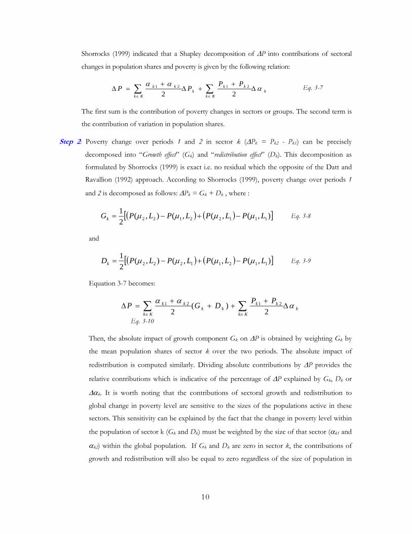
Shorrocks (1999) indicated that a Shapley decomposition of ∆P into contributions of sectoral
changes in population shares and poverty is given by the following relation:
kKk
kkk
Kk
kk PPPP α
αα∆
++∆
+=∆ ∑∑
∈∈ 222121 Eq. 3-7
The first sum is the contribution of poverty changes in sectors or groups. The second term is
the contribution of variation in population shares.
Step 2: Poverty change over periods 1 and 2 in sector k (∆Pk = Pk2 - Pk1) can be precisely
decomposed into “Growth effect” (Gk) and “redistribution effect” (Dk). This decomposition as
formulated by Shorrocks (1999) is exact i.e. no residual which the opposite of the Datt and
Ravallion (1992) approach. According to Shorrocks (1999), poverty change over periods 1
and 2 is decomposed as follows: ∆Pk = Gk + Dk , where :
( ) ( )[ ]),(,(,(),(21
11122122 LPLPLPLPGk µµµµ −+−= Eq. 3-8
and
( ) ( )[ ]),(,(,(),(21
11211222 LPLPLPLPDk µµµµ −+−= Eq. 3-9
Equation 3-7 becomes:
kKk
kkkk
Kk
kk PPDGP ααα∆
+++
+=∆ ∑∑
∈∈ 2)(
22121
Eq. 3-10
Then, the absolute impact of growth component Gk on ∆P is obtained by weighting Gk by
the mean population shares of sector k over the two periods. The absolute impact of
redistribution is computed similarly. Dividing absolute contributions by ∆P provides the
relative contributions which is indicative of the percentage of ∆P explained by Gk, Dk or
∆αk. It is worth noting that the contributions of sectoral growth and redistribution to
global change in poverty level are sensitive to the sizes of the populations active in these
sectors. This sensitivity can be explained by the fact that the change in poverty level within
the population of sector k (Gk and Dk) must be weighted by the size of that sector (αk1 and
αk2) within the global population. If Gk and Dk are zero in sector k, the contributions of
growth and redistribution will also be equal to zero regardless of the size of population in
10
sector k. On the other hand, if the size of the population of sector j is very small compared
to the rest of the population, its growth contribution to overall change in poverty level will
be small (j
jj G2
21 αα + ) despite the more significant change in poverty level (Gj, Dj) in this
sector.
Prior to the presentation of our findings obtained through this approach, we describe the data and
sectors relevant to achieve our objectives.
4 . DATA AND SECTOR CHARACTERISTICS
The two major data sources that we used are: (1) National Accounts (referred to as NAM) for
macroeconomic data and, (2) the two national household surveys (Enquêtes Prioritaires, referred to as
EP) on household living conditions. EP I for the year 1994 consists of a sample of 8,642 households
and EP II for 1998 has a sample of 8,478 households. In both surveys, a 2-step stratified sampling
procedure is used with several strata. This sample design will be taken into account for the
computation of standard deviations.
Furthermore, we chose to disaggregate into four types of sectoral decomposition that we will refer to
as E1 to E4. Set E1 is the usual economic sectors such as primary, secondary, service sectors
including other sectors used for unspecified social economic group. E2 characterizes regional
decomposition into seven regions or cities including West, South-Southwest, Central North, Central
South, North, other cities and Ouagadougou-Bobo. Set E2 can be seen as referring to a geographical
decomposition and in Burkina this decomposition is important as the poverty reduction strategy
paper is implemented in part on a regional basis. It was not possible to use the actual thirteen (13)
official regional divisions that existed in 1998 since these were created in 1996 after the 1994 survey.
Our decomposition is meant to differentiate between five large rural and two urban areas (E2) to
capture agro-climatic and infrastructural differences, which two important aspects of growth. E3
subdivides the primary sector of the E1 classification into agricultural and other primary sectors
(fishing and livestock). The other E1 groups are maintained to complete this decomposition. Lastly,
set E4 decomposes the agricultural sector into food crop sector and cotton sector while aggregating
all others sectors (non-agricultural sector). Thus, sets E1, E3, E4 have been defined by taking into
account standard macroeconomic sectors in which the household work and information found in the
HS.
11
5 . FINDINGS
5.1. Relation between Consumption, GDP and Poverty
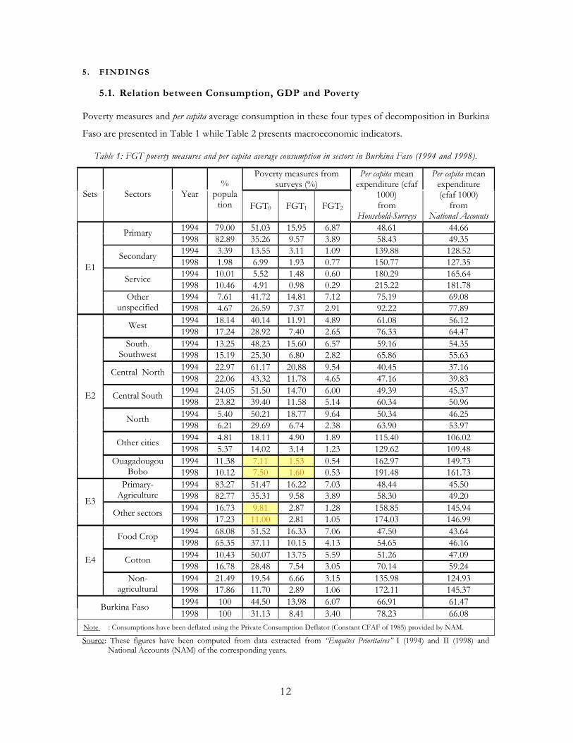
Poverty measures and per capita average consumption in these four types of decomposition in Burkina
Faso are presented in Table 1 while Table 2 presents macroeconomic indicators.
Table 1: FGT poverty measures and per capita average consumption in sectors in Burkina Faso (1994 and 1998).
Poverty measures from surveys (%)
Sets Sectors Year %
population FGT0 FGT1 FGT2
Per capita mean expenditure (cfaf
1000) from
Household-Surveys
Per capita mean expenditure (cfaf 1000)
from National Accounts
1994 79.00 51.03 15.95 6.87 48.61 44.66 Primary 1998 82.89 35.26 9.57 3.89 58.43 49.35 1994 3.39 13.55 3.11 1.09 139.88 128.52 Secondary 1998 1.98 6.99 1.93 0.77 150.77 127.35 1994 10.01 5.52 1.48 0.60 180.29 165.64 Service 1998 10.46 4.91 0.98 0.29 215.22 181.78 1994 7.61 41.72 14.81 7.12 75.19 69.08
E1
Other unspecified 1998 4.67 26.59 7.37 2.91 92.22 77.89
1994 18.14 40.14 11.91 4.89 61.08 56.12 West 1998 17.24 28.92 7.40 2.65 76.33 64.47 1994 13.25 48.23 15.60 6.57 59.16 54.35 South.
Southwest 1998 15.19 25.30 6.80 2.82 65.86 55.63 1994 22.97 61.17 20.88 9.54 40.45 37.16 Central North 1998 22.06 43.32 11.78 4.65 47.16 39.83 1994 24.05 51.50 14.70 6.00 49.39 45.37 Central South 1998 23.82 39.40 11.58 5.14 60.34 50.96 1994 5.40 50.21 18.77 9.64 50.34 46.25 North 1998 6.21 29.69 6.74 2.38 63.90 53.97 1994 4.81 18.11 4.90 1.89 115.40 106.02 Other cities 1998 5.37 14.02 3.14 1.23 129.62 109.48 1994 11.38 7.11 1.53 0.54 162.97 149.73
E2
Ouagadougou Bobo 1998 10.12 7.50 1.60 0.53 191.48 161.73
1994 83.27 51.47 16.22 7.03 48.44 45.50 Primary-Agriculture 1998 82.77 35.31 9.58 3.89 58.30 49.20
1994 16.73 9.81 2.87 1.28 158.85 145.94 E3
Other sectors 1998 17.23 11.00 2.81 1.05 174.03 146.99 1994 68.08 51.52 16.33 7.06 47.50 43.64 Food Crop 1998 65.35 37.11 10.15 4.13 54.65 46.16 1994 10.43 50.07 13.75 5.59 51.26 47.09 Cotton 1998 16.78 28.48 7.54 3.05 70.14 59.24 1994 21.49 19.54 6.66 3.15 135.98 124.93
E4
Non- agricultural 1998 17.86 11.70 2.89 1.06 172.11 145.37
1994 100 44.50 13.98 6.07 66.91 61.47 Burkina Faso 1998 100 31.13 8.41 3.40 78.23 66.08
Note : Consumptions have been deflated using the Private Consumption Deflator (Constant CFAF of 1985) provided by NAM.
Source: These figures have been computed from data extracted from “Enquêtes Prioritaires” I (1994) and II (1998) and National Accounts (NAM) of the corresponding years.
12
When comparing poverty indices between 1994 and 1998 and using 1985 CFA francs, poverty
incidence falls by about 30% (from 44.5% in 1994 to 31.13% in 1998), poverty gap falls by 40%
(13.98% to 8.41%) and poverty severity falls by 44% (6.07% to 3.40%) between 1994 and 1998.
These results are not independent of the 17% increase (66,910 Fcfa to 78,230 Fcfa) in the per capita
real expenditure calculated from the HS.
Looking at poverty dynamics by sector, we note that poverty incidence dropped by 11% in the service
sector (5.52% to 4.91%), by 31% in the primary sector (51.03% to 35.26%) and by 48% in the
secondary sector (13.55% to 6.99%) and in the South and South-West regions by 48.23% and 25.30%
respectively. Only two sectors witness worsening poverty incidence: (1) large cities: 5% increase in
Ouagadougou and Bobo Dioulasso (from 7.11% to 7.50%), and (2) non-agricultural sector of set E3:
with a 12% increase (going from 9,81% to 11%). From this we see that poverty changes are very
different from one sector to another.
The results presented in Table 1 also reveal that the per capita average expenditure is higher in HS
versus National Accounts (NAM) and this holds for all decompositions. National survey average is
8.85% higher than NAM’s average for 1994 and 18.39% for 1998. This result suggests that using
NAM consumption to evaluate poverty would result in higher poverty measures if the same nominal
poverty levels are used.
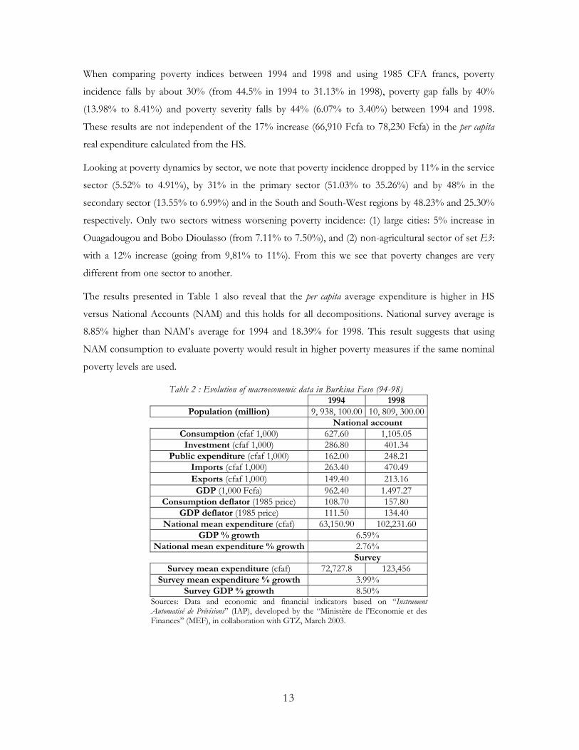
Table 2 : Evolution of macroeconomic data in Burkina Faso (94-98) 1994 1998
Population (million) 9, 938, 100.00 10, 809, 300.00 National account
Consumption (cfaf 1,000) 627.60 1,105.05 Investment (cfaf 1,000) 286.80 401.34
Public expenditure (cfaf 1,000) 162.00 248.21 Imports (cfaf 1,000) 263.40 470.49 Exports (cfaf 1,000) 149.40 213.16 GDP (1,000 Fcfa) 962.40 1.497.27
Consumption deflator (1985 price) 108.70 157.80 GDP deflator (1985 price) 111.50 134.40
National mean expenditure (cfaf) 63,150.90 102,231.60 GDP % growth 6.59%
National mean expenditure % growth 2.76% Survey
Survey mean expenditure (cfaf) 72,727.8 123,456 Survey mean expenditure % growth 3.99%
Survey GDP % growth 8.50% Sources: Data and economic and financial indicators based on “Instrument Automatisé de Prévisions” (IAP), developed by the “Ministère de l’Economie et des Finances” (MEF), in collaboration with GTZ, March 2003.
13
The upper part of Table 2 summarizes the main macroeconomic indicators of Burkina Faso for 1994
and 199812. The lower part shows the results obtained by combining national accounting data with
those calculated from HS. One can observe that all macroeconomic aggregates and the population
have grown between 94 and 98. Consumption and imports exhibit higher nominal increases at 76.1%
(627,600 Fcfa to 1,105,050 Fcfa) and 78.6% (263,400 Fcfa to 470,490 Fcfa) respectively. Public
expenditure follows with an increase of 53.2% and finally, investment and exports recorded the
smallest increase at 39.9% and 42.7% respectively. Furthermore, the consumer price index exhibited a
strong increase, which can be explained by the CFA franc devaluation in January 1994. The same
trend was observed for all countries of the zone (CFA zone). Since 1995, inflation and consumer
prices have remained relatively stable.
National mean expenditure describes the average consumption expenditure obtained from I-O table
(Cnam) divided by the size of Burkina Faso’s population as determined by the national population
census. The survey mean expenditure is obtained in the same way using Chs, or the total expenditure
figure provided by the household survey. We computed the growth rate of this aggregate by applying
the consumption deflator. Results revealed that the growth figure from the NAM was lower than the
HS figure at 2.76% compared to 3.99% for the HS. Using the same approach, we compared NAS
GDP (GDPnam) growth with HS GDP (GDPhs) growth and the result obtained follows the same
pattern. The economic growth rate is higher from HS data than NAM data (8.50% and 6.59%).
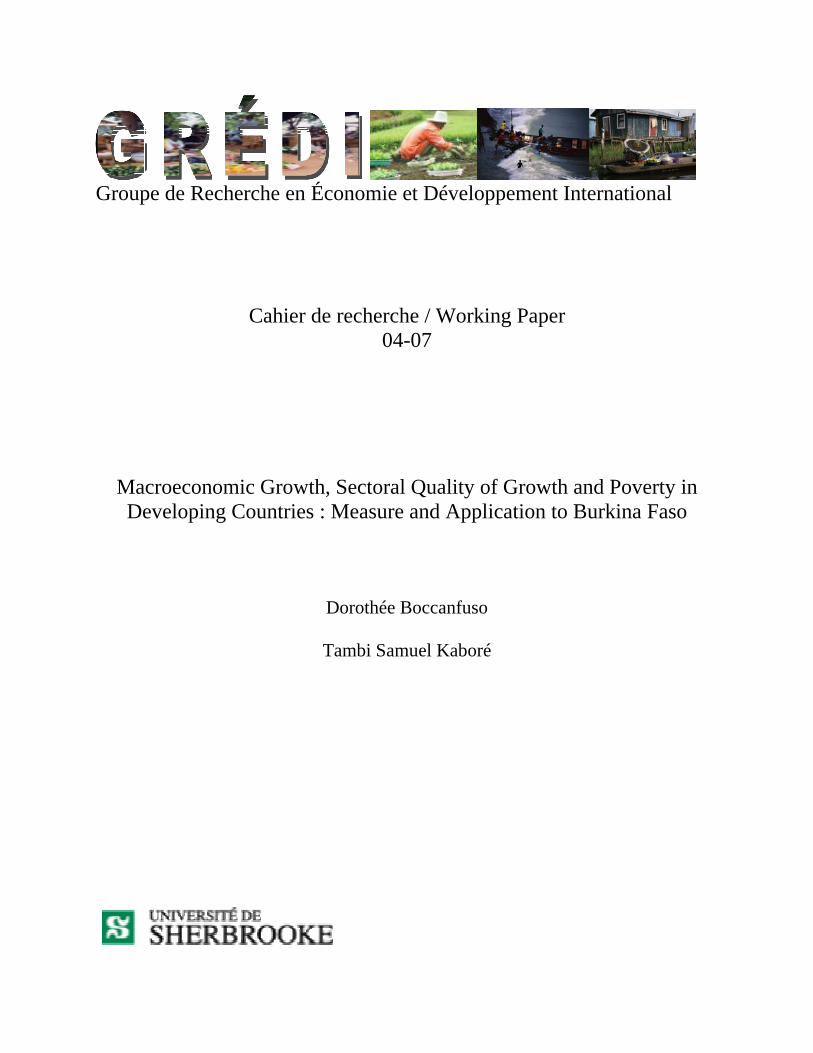
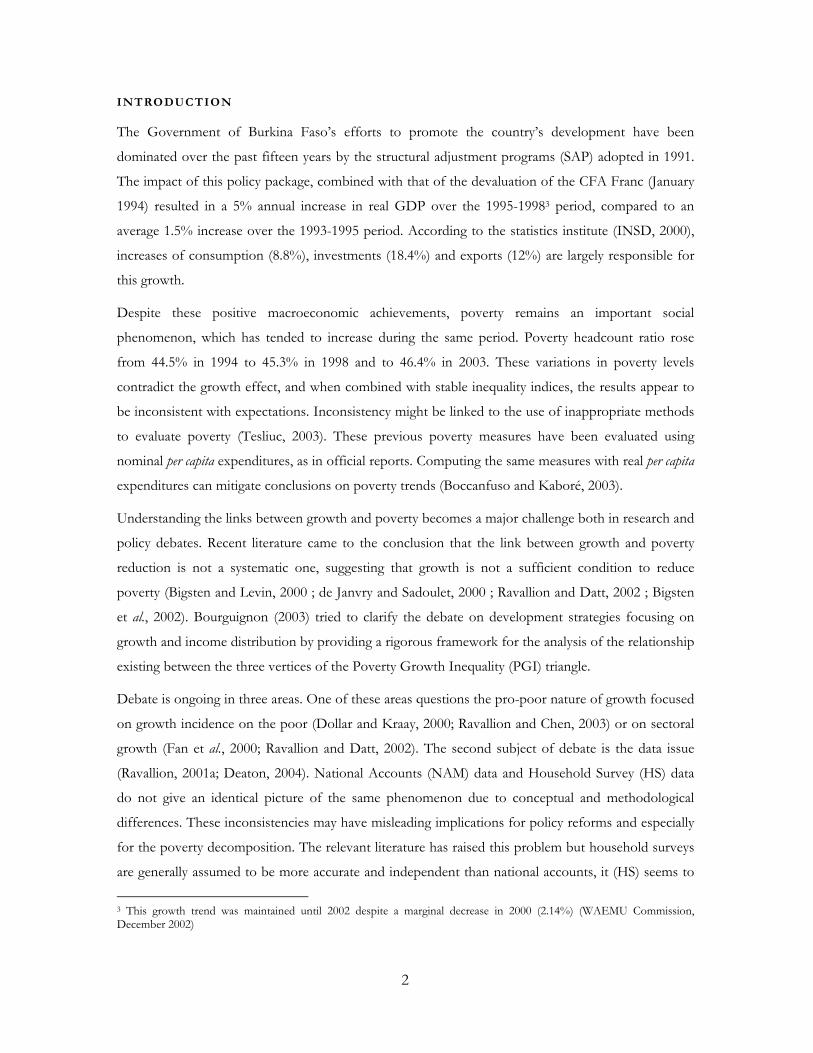
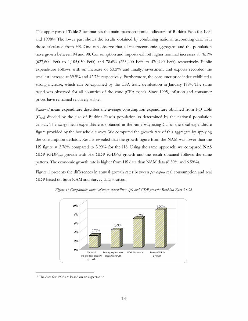
Figure 1 presents the differences in annual growth rates between per capita real consumption and real
GDP based on both NAM and Survey data sources.
Figure 1: Comparative table of mean expenditure (µ) and GDP growth: Burkina Faso 94-98
2,76%3,99%
6,59%
8,50%
0%
2%
4%
6%
8%
10%
Natio nalexpend iture mean %
growth
Survey exp end ituremean % g rowth
GDP % g ro wth Survey GDP %g ro wth
12 The data for 1998 are based on an expectation.
14
Two conclusions can be drawn from these results. The annual growth rate of per capita consumption
based on NAM (2.76%) is 44.56% smaller compared to the survey figure (3.99%). Similar difference
is observed in the GDP growth rate based on the total consumption figure provided by NAM
(6.59%) which is 28.98% smaller; compared to the GDP growth rate as computed on the basis of
survey total consumption figure (8.5%). On the other hand, using the per capita consumption growth
rate estimated on the basis of survey data as a proxy of economic growth rate, results in an under-
estimation of about 65.16% (3.99% compared to 6.59%).
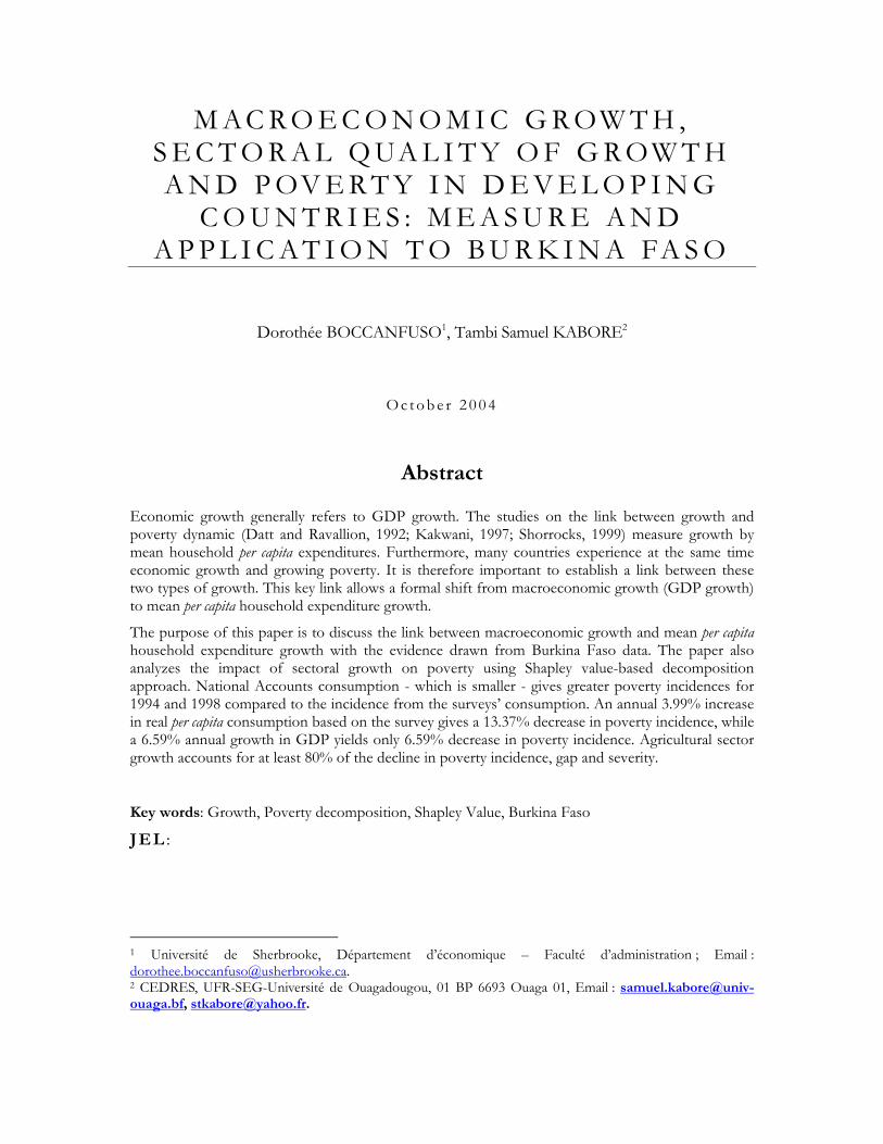
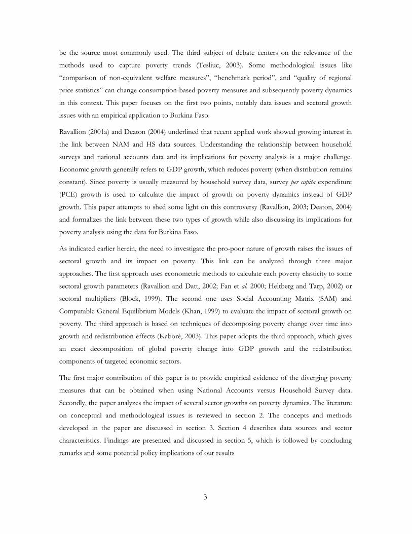
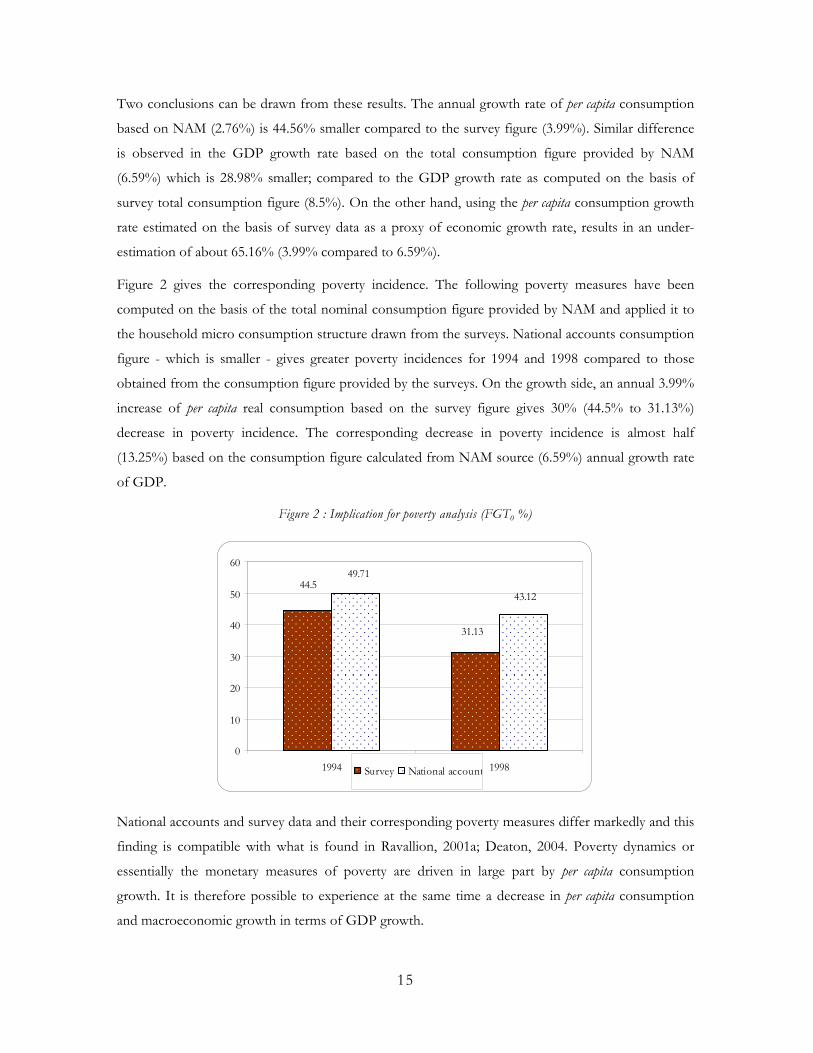
Figure 2 gives the corresponding poverty incidence. The following poverty measures have been
computed on the basis of the total nominal consumption figure provided by NAM and applied it to
the household micro consumption structure drawn from the surveys. National accounts consumption
figure - which is smaller - gives greater poverty incidences for 1994 and 1998 compared to those
obtained from the consumption figure provided by the surveys. On the growth side, an annual 3.99%
increase of per capita real consumption based on the survey figure gives 30% (44.5% to 31.13%)
decrease in poverty incidence. The corresponding decrease in poverty incidence is almost half
(13.25%) based on the consumption figure calculated from NAM source (6.59%) annual growth rate
of GDP.
Figure 2 : Implication for poverty analysis (FGT0 %)
44.5
31.13
49.71
43.12
0
10
20
30
40
50
60
1994 1998Survey National account
National accounts and survey data and their corresponding poverty measures differ markedly and this
finding is compatible with what is found in Ravallion, 2001a; Deaton, 2004. Poverty dynamics or
essentially the monetary measures of poverty are driven in large part by per capita consumption
growth. It is therefore possible to experience at the same time a decrease in per capita consumption
and macroeconomic growth in terms of GDP growth.
15
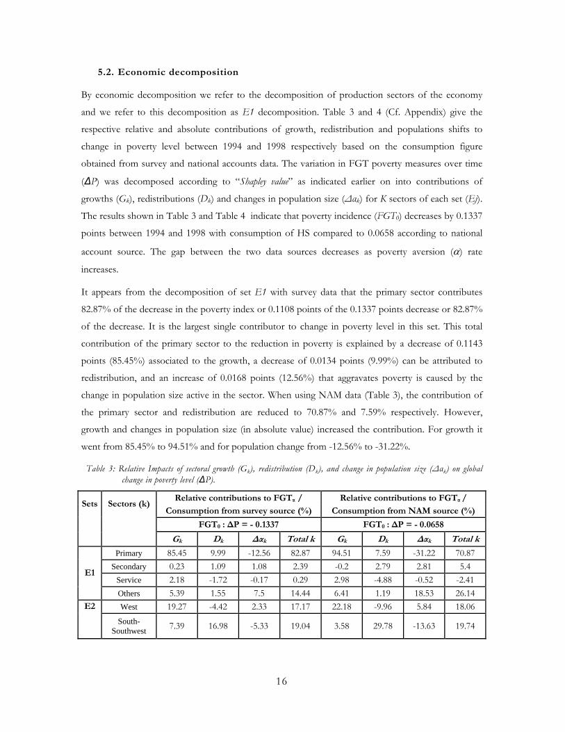
5.2. Economic decomposition
By economic decomposition we refer to the decomposition of production sectors of the economy
and we refer to this decomposition as E1 decomposition. Table 3 and 4 (Cf. Appendix) give the
respective relative and absolute contributions of growth, redistribution and populations shifts to
change in poverty level between 1994 and 1998 respectively based on the consumption figure
obtained from survey and national accounts data. The variation in FGT poverty measures over time
(∆P) was decomposed according to “Shapley value” as indicated earlier on into contributions of
growths (Gk), redistributions (Dk) and changes in population size (∆αk) for K sectors of each set (Ej).
The results shown in Table 3 and Table 4 indicate that poverty incidence (FGT0) decreases by 0.1337
points between 1994 and 1998 with consumption of HS compared to 0.0658 according to national
account source. The gap between the two data sources decreases as poverty aversion (α) rate
increases.
It appears from the decomposition of set E1 with survey data that the primary sector contributes
82.87% of the decrease in the poverty index or 0.1108 points of the 0.1337 points decrease or 82.87%
of the decrease. It is the largest single contributor to change in poverty level in this set. This total
contribution of the primary sector to the reduction in poverty is explained by a decrease of 0.1143
points (85.45%) associated to the growth, a decrease of 0.0134 points (9.99%) can be attributed to
redistribution, and an increase of 0.0168 points (12.56%) that aggravates poverty is caused by the
change in population size active in the sector. When using NAM data (Table 3), the contribution of
the primary sector and redistribution are reduced to 70.87% and 7.59% respectively. However,
growth and changes in population size (in absolute value) increased the contribution. For growth it
went from 85.45% to 94.51% and for population change from -12.56% to -31.22%.
Table 3: Relative Impacts of sectoral growth (Gk), redistribution (Dk), and change in population size (∆αk) on global change in poverty level (∆P).
Relative contributions to FGTα / Relative contributions to FGTα / Sets Sectors (k)
Consumption from survey source (%) Consumption from NAM source (%)
FGT0 : ∆P = - 0.1337 FGT0 : ∆P = - 0.0658
Gk Dk ∆αk Total k Gk Dk ∆αk Total k
Primary 85.45 9.99 -12.56 82.87 94.51 7.59 -31.22 70.87 Secondary 0.23 1.09 1.08 2.39 -0.2 2.79 2.81 5.4
Service 2.18 -1.72 -0.17 0.29 2.98 -4.88 -0.52 -2.41 E1
Others 5.39 1.55 7.5 14.44 6.41 1.19 18.53 26.14 West 19.27 -4.42 2.33 17.17 22.18 -9.96 5.84 18.06 E2
South-Southwest 7.39 16.98 -5.33 19.04 3.58 29.78 -13.63 19.74
16
Relative contributions to FGTα / Relative contributions to FGTα / Sets Sectors (k)
Consumption from survey source (%) Consumption from NAM source (%)
Central North 22.18 7.86 3.53 33.57 18.79 6.39 8.68 33.86 Central South 29.42 -7.76 0.78 22.45 35.75 -11.43 1.91 26.24
North 6.9 2.01 -2.41 6.5 8.45 3.62 -5.98 6.08 Other cities 1.53 0.03 -0.67 0.89 1.12 -1.13 -1.92 -1.93
Ouaga-Bobo 2.74 -3.06 0.69 0.38 3.75 -7.76 1.96 -2.05 Primary
agriculture 88.46 11.82 1.62 101.9 97.13 11.99 4.02 113.14 E3
Others 2.34 -3.85 -0.39 -1.9 0.62 -12.7 -1.06 -13.14 Crop food 53.35 18.54 9.01 80.9 46.25 20.3 22.4 88.94
Cotton 24.03 -2.07 -18.65 3.32 34.47 -3.03 -46.26 -14.82 E4 Non-
Agricultural 11.17 0.37 4.24 15.78 15.48 -0.46 10.85 25.88
FGT1 : ∆P = - 0.0557 FGT1 : ∆P = - 0.0384
Primary 81.62 11.21 -8.92 83.91 76.51 18.05 -17.04 77.52 Secondary 0.27 0.3 0.64 1.2 -0.06 0.85 1.27 2.05
Service 1.33 -0.4 -0.1 0.84 1.48 -1.17 -0.21 0.1 E1
Others 5.39 2.82 5.85 14.05 5.36 4.12 10.86 20.33 West 18.03 -3.68 1.56 15.91 18.97 -6.4 3.06 15.63
South-Southwest 7.15 15.32 -3.9 18.57 2.74 26.4 -7.36 21.78
Central North 22.71 14.09 2.65 39.45 17.39 20.59 4.98 42.96 Central South 26.57 -13.16 0.54 13.95 26.97 -19.66 1.04 8.35
North 700,00% 5.54 -1.85 10.69 7.55 8.03 -3.44 12.14 Other cities 1.27 0.33 -0.4 1.21 0.71 0.35 -0.83 0.23
E2
Ouaga-Bobo 1.71 -1.84 0.36 0.23 1.71 -3.6 0.79 -1.1 Primary
agriculture 84.69 14.23 1.16 100.07 79.72 22.77 2.2 104.69 E3
Others 2.17 -1.99 -0.25 -0.07 0.31 -4.49 -0.52 -4.69 Crop food 52.63 21.39 6.47 80.49 36.21 34.2 12.33 82.73
Cotton 20.67 -5.48 -12.14 3.05 26.67 -7.87 -23.69 -4.88 E4 Non-
Agricultural 9.25 4.09 3.11 16.46 10.71 5.57 5.88 22.16
FGT2 : ∆P = - 0.0266 FGT2 : ∆P = - 0.0204
Primary 82.11 8.58 -7.86 82.83 75.05 16.22 -14.13 77.14 Secondary 0.23 0.09 0.49 0.81 -0.05 0.36 0.94 1.24
Service 1.1 0.1 -0.07 1.12 1.1 -0.24 -0.15 0.71 E1
Others 5.73 3.99 5.53 15.24 5.53 5.82 9.56 20.91 West 17.34 -2.43 1.28 16.19 18.46 -4.94 2.4 15.91
South-Southwest 7.36 12.64 -3.42 16.58 2.67 23.18 -6.06 19.79
Central North 24.04 17.28 2.41 43.73 17.9 26.44 4.26 48.6
E2
Central South 26.92 -19.16 0.48 8.25 26.27 -27.8 0.87 -0.66
17
Relative contributions to FGTα / Relative contributions to FGTα / Sets Sectors (k)
Consumption from survey source (%) Consumption from NAM source (%)
North 7.13 8.7 -1.82 14.01 7.69 12.29 -3.08 16.9 Other cities 1.09 0.18 -0.32 0.95 0.56 0.38 -0.62 0.33
Ouaga-Bobo 1.37 -1.34 0.25 0.29 1.27 -2.68 0.54 -0.87 Primary
agriculture 85.47 12.26 1.02 98.76 78.46 21.89 1.83 102.19 E3
Others 1.98 -0.52 -0.22 1.24 0.28 -2.05 -0.41 -2.19 Crop food 53.57 19.69 5.71 78.98 35.95 34.03 10.27 80.25
Cotton 19.71 -6.72 -10.29 2.7 24.92 -10.29 -18.79 -4.17 E4 Non-
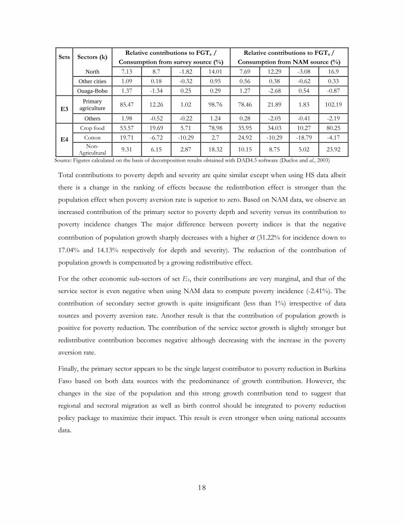
Agricultural 9.31 6.15 2.87 18.32 10.15 8.75 5.02 23.92 Source: Figures calculated on the basis of decomposition results obtained with DAD4.3 software (Duclos and al., 2003)
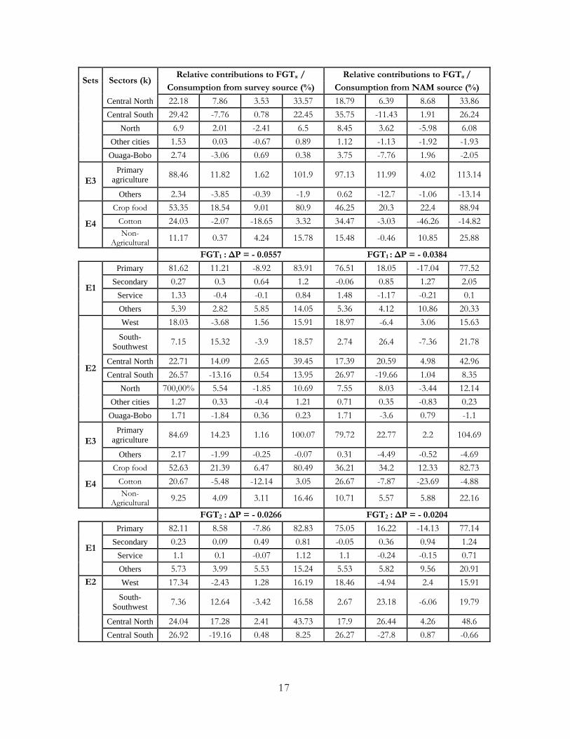
Total contributions to poverty depth and severity are quite similar except when using HS data albeit
there is a change in the ranking of effects because the redistribution effect is stronger than the
population effect when poverty aversion rate is superior to zero. Based on NAM data, we observe an
increased contribution of the primary sector to poverty depth and severity versus its contribution to
poverty incidence changes The major difference between poverty indices is that the negative
contribution of population growth sharply decreases with a higher α (31.22% for incidence down to
17.04% and 14.13% respectively for depth and severity). The reduction of the contribution of
population growth is compensated by a growing redistributive effect.
For the other economic sub-sectors of set E1, their contributions are very marginal, and that of the
service sector is even negative when using NAM data to compute poverty incidence (-2.41%). The
contribution of secondary sector growth is quite insignificant (less than 1%) irrespective of data
sources and poverty aversion rate. Another result is that the contribution of population growth is
positive for poverty reduction. The contribution of the service sector growth is slightly stronger but
redistributive contribution becomes negative although decreasing with the increase in the poverty
aversion rate.
Finally, the primary sector appears to be the single largest contributor to poverty reduction in Burkina
Faso based on both data sources with the predominance of growth contribution. However, the
changes in the size of the population and this strong growth contribution tend to suggest that
regional and sectoral migration as well as birth control should be integrated to poverty reduction
policy package to maximize their impact. This result is even stronger when using national accounts
data.
18
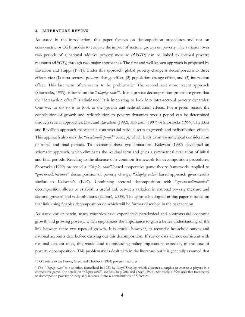
5.3. Regional decomposition
As announced earlier herein, we applied the decomposition approach to seven regions or cities since
geographic location is a key component of the global poverty reduction strategy especially in the
PRSP context. Figure 3 summarizes the FGT0 variation results presented in Table 3.
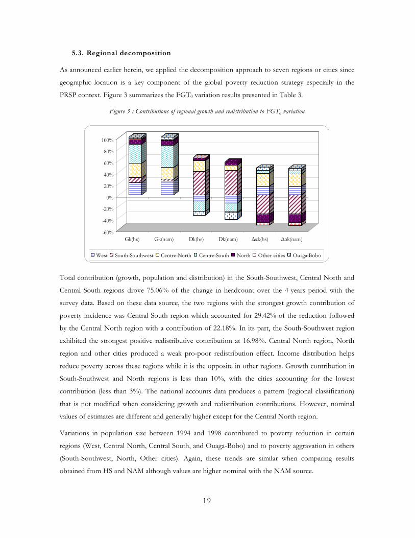
Figure 3 : Contributions of regional growth and redistribution to FGT0 variation
-60%
-40%
-20%
0%
20%
40%
60%
80%
100%
Gk(hs) Gk(nam) Dk(hs) Dk(nam) ∆αk(hs) ∆αk(nam)
West South-Southwest Centre-North Centre-South North Other cities Ouaga-Bobo
Total contribution (growth, population and distribution) in the South-Southwest, Central North and
Central South regions drove 75.06% of the change in headcount over the 4-years period with the
survey data. Based on these data source, the two regions with the strongest growth contribution of
poverty incidence was Central South region which accounted for 29.42% of the reduction followed
by the Central North region with a contribution of 22.18%. In its part, the South-Southwest region
exhibited the strongest positive redistributive contribution at 16.98%. Central North region, North
region and other cities produced a weak pro-poor redistribution effect. Income distribution helps
reduce poverty across these regions while it is the opposite in other regions. Growth contribution in
South-Southwest and North regions is less than 10%, with the cities accounting for the lowest
contribution (less than 3%). The national accounts data produces a pattern (regional classification)
that is not modified when considering growth and redistribution contributions. However, nominal
values of estimates are different and generally higher except for the Central North region.
Variations in population size between 1994 and 1998 contributed to poverty reduction in certain
regions (West, Central North, Central South, and Ouaga-Bobo) and to poverty aggravation in others
(South-Southwest, North, Other cities). Again, these trends are similar when comparing results
obtained from HS and NAM although values are higher nominal with the NAM source.
19
The previous pattern of growth, redistribution and population change (signs of impacts and regional
ranking) was maintained for poverty gap (FGT1) and severity (FGT2). However, it is not possible to
infer on the dominance of contributions when comparing the two data sources. In some instances,
contributions from one data source dominate the other and in other cases it is the other data source
results that dominate.
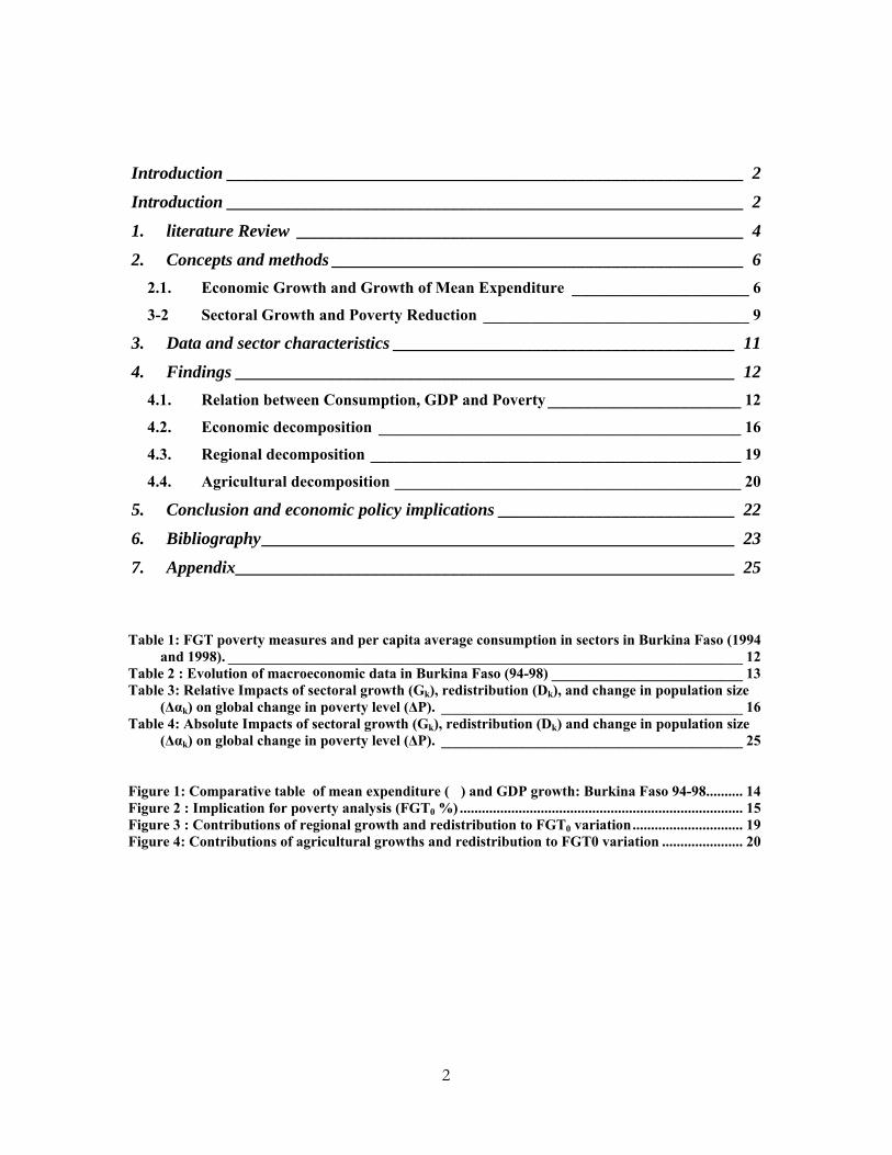
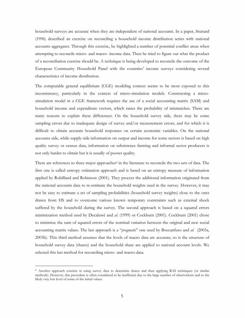
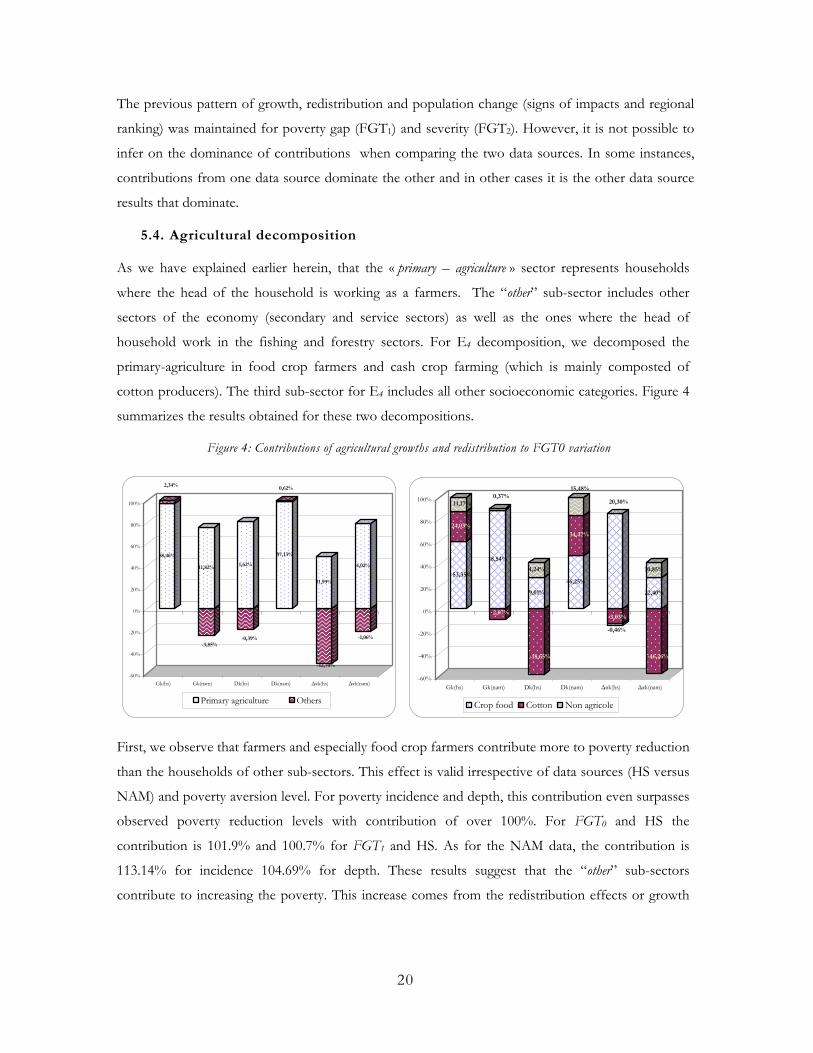
5.4. Agricultural decomposition
As we have explained earlier herein, that the « primary – agriculture » sector represents households
where the head of the household is working as a farmers. The “other” sub-sector includes other
sectors of the economy (secondary and service sectors) as well as the ones where the head of
household work in the fishing and forestry sectors. For E4 decomposition, we decomposed the
primary-agriculture in food crop farmers and cash crop farming (which is mainly composted of
cotton producers). The third sub-sector for E4 includes all other socioeconomic categories. Figure 4
summarizes the results obtained for these two decompositions.
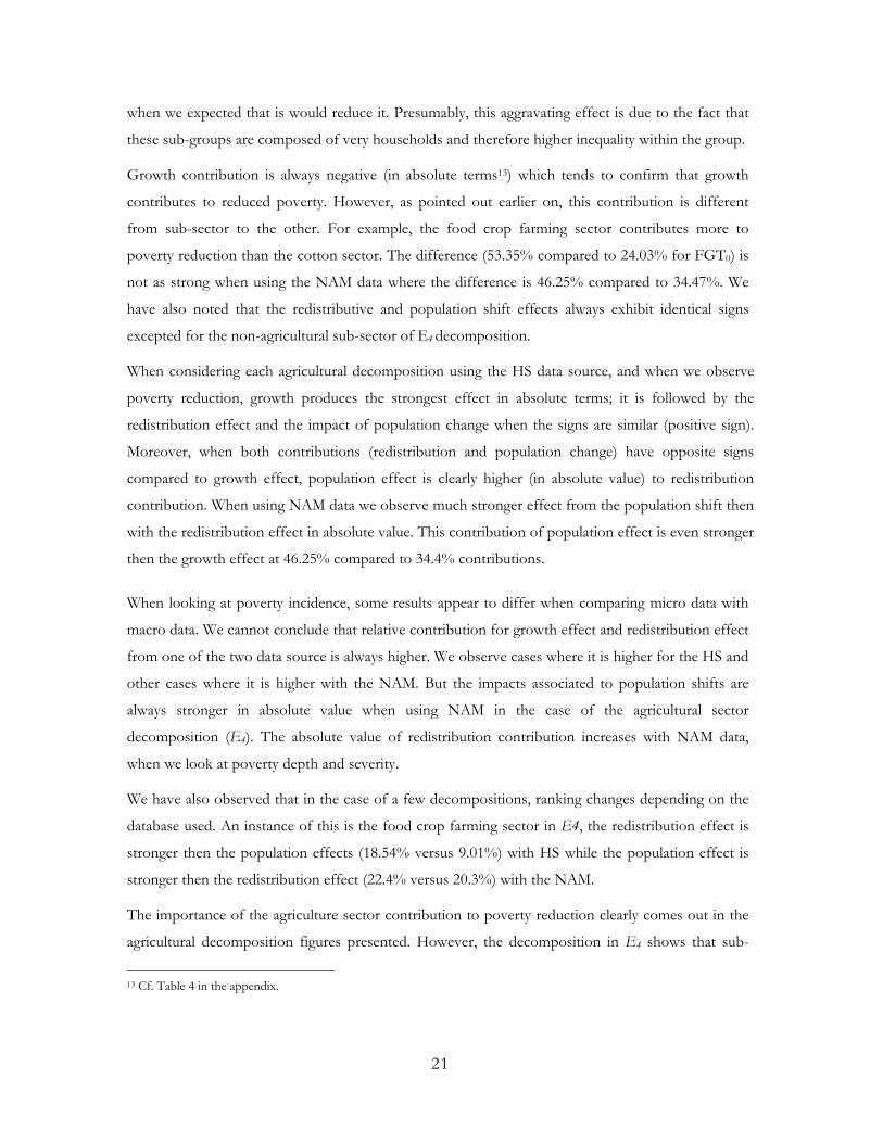
Figure 4: Contributions of agricultural growths and redistribution to FGT0 variation
88,46%
2,34%
11,82%
-3,85%
1,62%
-0,39%
97,13%
0,62%
11,99%
-12,70%
4,02%
-1,06%
-60%
-40%
-20%
0%
20%
40%
60%
80%
100%
Gk(hs) Gk(nam) Dk(hs) Dk(nam) ∆αk(hs) ∆αk(nam)
Primary agriculture Others
53,35%
24,03%
11,17%
18,54%
-2,07%
0,37%
9,01%
-18,65%
4,24%
46,25%
34,47%
15,48%
20,30%
-3,03%
-0,46%
22,40%
-46,26%
10,85%
-60%
-40%
-20%
0%
20%
40%
60%
80%
100%
Gk(hs) Gk(nam) Dk(hs) Dk(nam) ∆αk(hs) ∆αk(nam)
Crop food Cotton Non agricole
First, we observe that farmers and especially food crop farmers contribute more to poverty reduction
than the households of other sub-sectors. This effect is valid irrespective of data sources (HS versus
NAM) and poverty aversion level. For poverty incidence and depth, this contribution even surpasses
observed poverty reduction levels with contribution of over 100%. For FGT0 and HS the
contribution is 101.9% and 100.7% for FGT1 and HS. As for the NAM data, the contribution is
113.14% for incidence 104.69% for depth. These results suggest that the “other” sub-sectors
contribute to increasing the poverty. This increase comes from the redistribution effects or growth
20
when we expected that is would reduce it. Presumably, this aggravating effect is due to the fact that
these sub-groups are composed of very households and therefore higher inequality within the group.
Growth contribution is always negative (in absolute terms13) which tends to confirm that growth
contributes to reduced poverty. However, as pointed out earlier on, this contribution is different
from sub-sector to the other. For example, the food crop farming sector contributes more to
poverty reduction than the cotton sector. The difference (53.35% compared to 24.03% for FGT0) is
not as strong when using the NAM data where the difference is 46.25% compared to 34.47%. We
have also noted that the redistributive and population shift effects always exhibit identical signs
excepted for the non-agricultural sub-sector of E4 decomposition.
When considering each agricultural decomposition using the HS data source, and when we observe
poverty reduction, growth produces the strongest effect in absolute terms; it is followed by the
redistribution effect and the impact of population change when the signs are similar (positive sign).
Moreover, when both contributions (redistribution and population change) have opposite signs
compared to growth effect, population effect is clearly higher (in absolute value) to redistribution
contribution. When using NAM data we observe much stronger effect from the population shift then
with the redistribution effect in absolute value. This contribution of population effect is even stronger
then the growth effect at 46.25% compared to 34.4% contributions.
When looking at poverty incidence, some results appear to differ when comparing micro data with
macro data. We cannot conclude that relative contribution for growth effect and redistribution effect
from one of the two data source is always higher. We observe cases where it is higher for the HS and
other cases where it is higher with the NAM. But the impacts associated to population shifts are
always stronger in absolute value when using NAM in the case of the agricultural sector
decomposition (E4). The absolute value of redistribution contribution increases with NAM data,
when we look at poverty depth and severity.
We have also observed that in the case of a few decompositions, ranking changes depending on the
database used. An instance of this is the food crop farming sector in E4, the redistribution effect is
stronger then the population effects (18.54% versus 9.01%) with HS while the population effect is
stronger then the redistribution effect (22.4% versus 20.3%) with the NAM.
The importance of the agriculture sector contribution to poverty reduction clearly comes out in the
agricultural decomposition figures presented. However, the decomposition in E4 shows that sub-
13 Cf. in the appendix. Table 4
21
sectors don’t have the same relative contribution and to implement the most efficient poverty
reduction policies needs to go beyond low level of decomposition used in E3. For instance, food
crop farmers contribute strongly to poverty reduction while the “cotton” sector farmers barely
contribute (3.32%) when using HS. If we use NAM, cotton farmers don’t contribute to reduce
poverty but contribute to aggravate it (+14.82%). On these grounds, one can suggest focusing on
food-crop to achieve pro-growth and pro-poor policies. This should be done in combination to
controlling population growth such as birth control, regional or sectoral migration policies to
mitigate the negative impact they have on poverty incidence.
6 . CONCLUSION AND ECONOMIC POLICY IMPLICATIONS
This purpose of this paper is to discuss the impact of doing growth-inequality-poverty analysis with
two types of data sources such as – National Accounts (NAM) versus Households Surveys (HS) –
and the effects of sectoral growth on poverty analysis. Based on different consumption figures in HS
and NAM data, poverty measured on these two data source were also different . NAM consumption
figure - which is smaller than HS - gives greater poverty incidences for 1994 and 1998 than those of
NAM. In terms of growth, an annual 3.99% increase in HS per capita real consumption generates a
13.37% decrease in poverty incidence. The corresponding decrease in poverty incidence is twice
smaller (6.59%) based on NAM figures and the equivalent annual GDP growth of 6.59%. The major
force behind poverty dynamics, is the growth of HS per capita consumption. It is therefore possible to
experience at the same time a decrease in HS per capita consumption and macroeconomic (GDP)
growth. To have an effective impact on poverty reduction, economic growth (GDP) should be driven
by the per capita household consumption or income growth. One of the questions raised is what kind
of sectoral growth is most beneficial to the poor? This question was examined through a sectoral
decomposition of poverty variation over time with the two data sources.
Many economic sectors have been considered in this analysis. Primary sector growth alone accounted
for 85.45% of the change in poverty incidence between 1994 and 1998 in Burkina Faso. With NAM
figures, the contribution of primary sector growth dropped to 75.05%. The results obtained for
regional decomposition indicated that 70.87% of the change in poverty headcount ratio between 1994
and 1998 was driven by growth in three regions (Central South, Central North and West). The growth
contribution of each of the other regions is less than 15%. Cities accounted for the lowest growth
contribution (less than 3%). Primary agricultural sector growth accounted for 88.46% of the decrease
in poverty incidence. Looking at agricultural sub-sectors, the results indicated that food crop sub-
sector growth accounted for 53.35% of the change in poverty headcount ratio while the cotton sector
growth was responsible for 24.04% change in headcount. However, redistribution impact is negative
22
to the poor in the cotton sub-sector. The results highlighted the importance of the agricultural sector
in poverty reduction strategies. The important role played by the agricultural sector in the promotion
of economic growth and poverty reduction was also demonstrated in Ethiopia (Block, 1999), and
South Africa (Khan, 1999).
Two major lessons can be drawn from the results. The first lesson is that micro side growth, no
matter whether its per capita consumption or income is low, generally contributes more largely to a
decline in poverty than stronger macroeconomic growth. Secondly, the agricultural sector plays an
important role in poverty reduction. Focusing in the agricultural sector on food crop sub-sector will
result at least in 80% drop in poverty incidence, gap and severity. The importance of this food crop
sub-sector can be explained by the fact that it produces the pro-poor distribution and population shift
effects that reinforces positive growth impact. In the cotton sub-sector, only growth impact entails
poverty reduction. Redistribution and population variations increase poverty in the cotton sub-sector
and therefore reduce the global impact of the sub-sector on poverty reduction.
7 . BIBLIOGRAPHY
Banque Mondiale, 2000. Rapport sur le développement dans le monde 1998-1999 : le savoir au service du développement. Editions ESKA.
Bigsten, A. ; Levin J., 2000. Growth, Income Distribution and Poverty : A review. Working Paper in Economics N°32. JEL-Classification 01, 02. Göteborg University.
Bigsten A. ; Kebede, B. ; Shimeles, A. and Taddesse, M., 2002. Growth and Poverty in Ethiopia : Evidence from Household Panel Surveys. World Development Vol. 31, N°1, pp 87-106.
Block, S., A., 1999. Agricultural and Economic Growth in Ethiopia : Growth multipliers from a four-sector simulation model. Agricultural Economics 20 (1999) 241-252.
Boccanfuso, D. and S. T. Kaboré, 2003. Croissance, Inégalité et Pauvreté dans les Années 1990 au Burkina Faso et au Sénégal, To be published in « Revue d’Economie du Développement ».
Boccanfuso, D., B. Decaluwé and L. Savard, (2003a) " Poverty, Income Distribution and CGE modeling: Does the Functional Form of Distribution Matter?" Papier présenté à la conférence WIDER sur «Pauvreté, Équité et Bien-être», Helsinki, May 2003.
Boccanfuso D., F. Cabral, F. Cissé, A. Diagne and L. Savard, (2003b), « Pauvreté et distribution de revenus au Sénégal : une approche par la modélisation en équilibre général calculable micro-simulé »
Cockburn, J. (2001), « Trade liberalization and Poverty in Nepal: A Computable General Equilibrium Micro-simulation Analysis », Working paper 01-18. CREFA, Université Laval.
Datt, G. and M. Ravallion, 1992. Growth and Redistribution Components of Changes in Poverty Measures : A decomposition with applications to Brazil and India in 1980s. Journal of Development Economics, 38 (1992) 275-295.
Deaton, A., 2004. Measuring Poverty in a Growing World (or Measuring growth in a poor World), Princeton University. Miméo.
23
Decaluwé, B., J.C. Dumont and L. Savard (1999), « How to Measure Poverty and Inequality in General Equilibrium Framework », Laval University, CREFA Working Paper #9920.
de Janvry, A. and Sadoulet E., 2000. Growth, Inequality and Poverty in Latin America : a causal analysis, 1970-1994. Review of Income and Wealth, Vol.46, N°3 (sept 2000).
Duclos, J.-Y., A. Araar and C. Fortin, 2003. « DAD : un logiciel d’analyse distributive», CIRPÉE, Université Laval, et le Réseau MIMAP, CRDI (téléchargeable gratuitement à l’adresse www.mimap.ecn.ulaval.ca), 2003
Fan, S.; Hazell, P. and T. Haque, 2000. Targeting Public Investment by Agro-ecological zone to Achieve Growth and Poverty Alleviation Goals in Rural India. Food Policy 25 (2000) 411- 428.
Foster, J. ; Greer, J. and E. Thorbecke, 1984. A Class of Decomposable Poverty Measures. Econometrica 52, 761-765.
Heltberg, R. and F. Tarp, 2002. Agricultural Supply Response and Poverty in Mozambique. Food Policy 27 (2002) 103-124.
Kaboré O. F., 1993. Profil de la Pauvreté au Burkina Faso, Juin 1993. Photocopie
Kaboré, S. T., 2003. Qualité de la croissance économique et pauvreté dans les pays en développement: mesure et application au Burkina Faso. forthcoming in « Revue d’Economie du Développement ».
Kakwani, N., 1997. On measuring Growth and Inequality Components of Poverty with Application to Thailand. Discussion Paper. School of Economics, The University of New South Wales.
Khan, H., A., 1999. Sectoral Growth and Poverty Alleviations : A multiplier Decomposition Technique Applied to South Africa. World Development Vol. 27, N°3, pp 521-530.
Kuznets, S., 1955. « Economic Growth and Income Inequality », American Economic Review, 45.
INSD, 1996a. Analyse des Résultats de l’Enquête Prioritaire sur les Conditions de Vie des Ménages. Ministère de l’Economie, des Finances et du Plan; Projet d’Appui Institutionnel aux Dimensions Sociales de l’Ajustement.
INSD, 1996b. Le Profil de Pauvreté au Burkina Faso. Ministère de l’Economie, des Finances et du Plan; Projet d’Appui Institutionnel aux Dimensions Sociales de l’Ajustement.
INSD, 2000a. Analyse des Résultats de l’Enquête Prioritaire sur les Conditions de Vie des Ménages en 1998. Ministère de l’Economie et des Finances; Direction des Statistiques Générales, Etude Statistique Nationale, Première Edition, Ouagadougou, Mars 2000.
INSD, 2000b. Profil et Evolution de la Pauvreté au Burkina Faso. Ministère de l’Economie et des Finances; Direction des Statistiques Générales, Etude Statistique Nationale, Première Edition, Ouagadougou, Mars 2000.
Lachaud, J-P, 1996. Croissance Economique, Pauvreté et Inégalité des Revenus en Afrique Subsaharienne : Analyse comparative, Bordeaux, DT/11, Centre d’Economie du Développement, Université Montesquieu-Bordeaux IV.
Moulin, H., 1988. Axioms of Cooperative Decision Making. Cambridge University Press.
Owen, G. ; 1977. Values of Games with a Priori Unions ; In Mathematical Economics and Game Theory : Essays in Honor of Oskar Morgenstern, Henn, R. ; Moeschlin (Springer-Verlag, Berlin-Heidelberg-New York)
Ravallion, M., 2001a. Measuring Aggregate Welfare in Developing Countries : How well do National Accounts and Surveys Agree ? Working Paper, Jel. C80, E21, I31.
24
Ravallion, M., 2001b. Growth, Inequality and Poverty : Looking Beyond Averages. World Development Vol. 29, N°11, pp 1803-1815.
Ravallion M., 1996. Comparaisons de la Pauvreté, Concepts et Méthodes. LSMS document de travail N°122. Banque Mondiale, Washington, D.C.
Ravallion M. and S. Chen , 2003. Measuring pro-poor growth. Economics Letters 78 (2003) 93-99.
Ravallion M.and G. Datt, 2002. Why has Economic Growth been more Pro-poor in some states of India than others ? Journal of Development Economics, 68 (2002) 381-400.
Ravallion M. and M. Huppi, 1991. Measuring Changes in Poverty : A Methodological Case Study of Indonesia during an Adjustment Period. The World Bank Economic Review. Vol. 5, N°1, 57-82., Document de travail N°122. Banque Mondiale, Washington, D.C.
Savadogo, K., Ouédraogo, J.B. and T. Thiombiano, 1995. Profil de la pauvreté au Burkina Faso: Une approche qualitative et quantitative. Rapport soumis à la Banque Mondiale, version provisoire.
Sawadogo, K., 1997. La pauvreté au Burkina Faso : une analyse critique des politiques et des stratégies d’intervention locales. ECDPM Document de travail n°51
Shorrocks, A.F.; 1999. Decomposition Procedures for Distributional Analysis : A Unified Framework Based on the Shapley Value. Mimeo. Department of Economics, University of Essex.
Stuttard, N., 1996 Reconciliation of UK Household Income Statistics with the National Accounts, presented at the Meeting of the Expert Group on Household Income Statistics, Canberra (Australia), 2-4 December 1996.
Tesliuc E.D., 2003. Burkina Faso : Quo Vadis Poverty ? Banque Mondiale, Photocopie.
Wetta, C. ; Kaboré T.S. ; Bonzi K.B. ; Sikirou, S. ; Sawadogo M. and P. Somda, 1999. Profil d’inégalité et de pauvreté au Burkina Faso. Cahiers de Recherche du CREFA, N° : 00-02, Jel : D33, I32, Université Laval, Québec.
8 . APPENDIX
Table 4: Absolute Impacts of sectoral growth (Gk), redistribution (Dk) and change in population size (∆αk) on global change in poverty level (∆P).
Absolute contributions to FGTα / Consumption from survey source
Absolute Contributions to FGTα / Consumption from NAM source
FGT0 : ∆P = - 0,1337 FGT0 : ∆P = - 0,0658 Sets Sectors
Gk Dk ∆αk Total k Gk Dk ∆αk Total k
Primary -01143 -0,0134 0,0168 -0,1108 -0,0622 -0,0050 0,0206 -0,0467
Secondary -0,0003 -0,0015 -0,0014 -0,0032 0,0001 -0,0018 -0,0019 -0,0036
Service -0,0029 0,0023 0,0002 -0,0004 -0,0020 0,0032 0,0003 0,0016 E1
Others -0,0072 -0,0021 -0,0100 -0,0193 -0,0042 -0,0008 -0,0122 -0,0172
West -0,0258 0,0059 -0,0031 -0,0230 -0,0146 0,0066 -0,0038 -0,0119
South-Southwest -0,0099 -0,0227 0,0071 -0,0255 -0,0024 -0,0196 0,0090 -0,0130
Central North -0,0297 -0,0105 -0,0047 -0,0449 -0,0124 -0,0042 -0,0057 -0,0223
Central South -0,0393 0,0104 -0,0010 -0,0300 -0,0235 0,0075 -0,0013 -0,0173
E2
North -0,0092 -0,0027 0,0032 -0,0087 -0,0056 -0,0024 0,0039 -0,0040
25
Absolute contributions to FGTα / Consumption from survey source
Absolute Contributions to FGTα / Consumption from NAM source
FGT0 : ∆P = - 0,1337 FGT0 : ∆P = - 0,0658 Sets Sectors
Gk Dk ∆αk Total k Gk Dk ∆αk Total k
Other cities -0,0020 0,0000 0,0009 -0,0012 -0,0007 0,0007 0,0013 0,0013
Ouaga-Bobo -0,0037 0,0041 -0,0009 -0,0005 -0,0025 0,0051 -0,0013 0,0014 Primary -
agriculture -0,1183 -0,0158 -0,0022 -0,1363 -0,0640 -0,0079 -0,0026 -0,0745 E3
Others -0,0031 0,0051 0,0005 0,0025 -0,0004 0,0084 0,0007 0,0087
Food Crop -0,0713 -0,0248 -0,0121 -0,1082 -0,0305 -0,0134 -0,0147 -0,0586
Cotton -0,0321 0,0028 0,0249 -0,0044 -0,0227 0,0020 0,0305 0,0098 E4 Non-
Agricultural -0,0149 -0,0005 -0,0057 -0,0211 -0,0102 0,0003 -0,0071 -0,0170
FGT1 : ∆P = - 0,0557 FGT1 : ∆P = - 0,0384
Primary -0,0455 -0,0062 0,0050 -0,0467 -0,0294 -0,0069 0,0065 -0,0298
Secondary -0,0002 -0,0002 -0,0004 -0,0007 0,0000 -0,0003 -0,0005 -0,0008
Service -0,0007 0,0002 0,0001 -0,0005 -0,0006 0,0005 0,0001 0,0000 E1
Others -0,0030 -0,0016 -0,0033 -0,0078 -0,0021 -0,0016 -0,0042 -0,0078
West -0,0100 0,0021 -0,0009 -0,0089 -0,0073 0,0025 -0,0012 -0,0060 South-
Southwest -0,0040 -0,0085 0,0022 -0,0103 -0,0011 -0,0101 0,0028 -0,0084
Central North -0,0126 -0,0078 -0,0015 -0,0220 -0,0067 -0,0079 -0,0019 -0,0165
Central South -0,0148 0,0073 -0,0003 -0,0078 -0,0104 0,0076 -0,0004 -0,0032
North -0,0039 -0,0031 0,0010 -0,0060 -0,0029 -0,0031 0,0013 -0,0047
Other cities -0,0007 -0,0002 0,0002 -0,0007 -0,0003 -0,0001 0,0003 -0,0001
E2
Ouaga-Bobo -0,0010 0,0010 -0,0002 -0,0001 -0,0007 0,0014 -0,0003 0,0004 Primary -
agriculture -0,0472 -0,0079 -0,0006 -0,0557 -0,0306 -0,0087 -0,0008 -0,0402 E3
Others -0,0012 0,0011 0,0001 0,0000 -0,0001 0,0017 0,0002 0,0018
Food Crop -0,0293 -0,0119 -0,0036 -0,0448 -0,0139 -0,0131 -0,0047 -0,0318
Cotton -0,0115 0,0031 0,0068 -0,0017 -0,0102 0,0030 0,0091 0,0019 E4 Non-
Agricultural -0,0052 -0,0023 -0,0017 -0,0092 -0,0041 -0,0021 -0,0023 -0,0085
FGT2 : ∆P = - 0,0266 FGT2 : ∆P = - 0,0204
Primary -0,0219 -0,0023 0,0021 -0,0221 -0,0153 -0,0033 0,0029 -0,0157
Secondary -0,0001 0,0000 -0,0001 -0,0002 0,0000 -0,0001 -0,0002 -0,0003
Service -0,0003 0,0000 0,0000 -0,0003 -0,0002 0,0000 0,0000 -0,0001 E1
Others -0,0015 -0,0011 -0,0015 -0,0041 -0,0011 -0,0012 -0,0019 -0,0043
West -0,0046 0,0006 -0,0003 -0,0043 -0,0038 0,0010 -0,0005 -0,0032 South-
Southwest -0,0020 -0,0034 0,0009 -0,0044 -0,0005 -0,0047 0,0012 -0,0040
E2
Central North -0,0064 -0,0046 -0,0006 -0,0116 -0,0036 -0,0054 -0,0009 -0,0099
26

Absolute contributions to FGTα / Consumption from survey source
Absolute Contributions to FGTα / Consumption from NAM source
FGT0 : ∆P = - 0,1337 FGT0 : ∆P = - 0,0658 Sets Sectors
Gk Dk ∆αk Total k Gk Dk ∆αk Total k
Central South -0,0072 0,0051 -0,0001 -0,0022 -0,0053 0,0057 -0,0002 0,0001
North -0,0019 -0,0023 0,0005 -0,0037 -0,0016 -0,0025 0,0006 -0,0034
Other cities -0,0003 0,0000 0,0001 -0,0003 -0,0001 -0,0001 0,0001 -0,0001
Ouaga-Bobo -0,0004 0,0004 -0,0001 -0,0001 -0,0003 0,0005 -0,0001 0,0002 Primary -
agriculture -0,0228 -0,0033 -0,0003 -0,0263 -0,0160 -0,0045 -0,0004 -0,0208 E3
Others -0,0005 0,0001 0,0001 -0,0003 -0,0001 0,0004 0,0001 0,0004
Food Crop -0,0143 -0,0052 -0,0015 -0,0210 -0,0073 -0,0069 -0,0021 -0,0163
Cotton -0,0053 0,0018 0,0027 -0,0007 -0,0051 0,0021 0,0038 0,0008 E4
Non Agricole -0,0025 -0,0016 -0,0008 -0,0049 -0,0021 -0,0018 -0,0010 -0,0049 Source: Figures calculated from the decomposition results obtained with DAD4.3 software (Duclos and al., 2003).
27
Recommended