Ver 1.0 © Chua Kah Hean xmphysics 1
XMLECTURE
08 OSCILLATION NO DEFINITIONS. JUST PHYSICS.
8.1 Simple Harmonic Motion ............................................................................................................. 2
8.1.1 SHM in time-domain ............................................................................................................. 3
8.1.2 SHM in the x-domain ............................................................................................................ 4
8.1.3 The Half-Amplitude Problems ............................................................................................... 6
8.2 Restoring Force .......................................................................................................................... 7
8.2.1 Natural Frequency ................................................................................................................ 9
8.3 Energy of Oscillation ................................................................................................................. 11
8.3.1 SHM Energy in time-domain ............................................................................................... 13
8.3.2 SHM Energy in the x-domain .............................................................................................. 15
8.4 Damped Oscillations ................................................................................................................. 16
8.4.1 Practical Applications of Damping ...................................................................................... 19
8.5 Forced Oscillation ..................................................................................................................... 20
8.5.1 Resonance Curve ............................................................................................................... 22
8.5.2 Effect of Damping on Resonance ....................................................................................... 23
8.A Angular Frequency vs Angular Velocity .................................................................................... 25
8.B More Demonstrations ............................................................................................................... 26
Online resources are provided at https://xmphysics.com/osc

Ver 1.0 © Chua Kah Hean xmphysics 2
8.1 Simple Harmonic Motion
An oscillation such as a pendulum is fun to watch. When displaced and released, the pendulum will
go into a periodic to-and-fro motion about its equilibrium position. It’s always rushing towards the
equilibrium position, but overshoots every time, and is doomed to repeat this motion for eternity (until
its energy is totally sapped by resistive forces).
The pendulum (at small amplitude) and the spring-mass system are two examples of simple harmonic
motions (SHM). SHM is “simple” in the sense that its motion can be described by one single sinusoidal
function.
see animation at xmphysics.com
Specifically, the displacement x of a SHM with amplitude x0 and period T can be described by the
equation
0
2sinxx t
T
Math buffs may recognise the 2
T
term as the scaling factor that makes one cycle occupy one
period T. In physics, this 2
T
term is given the name angular frequency ω.
22 f
T
The angular frequency is a rather abstract concept which takes time to fully understand. For the time
being, it is sufficient to think of it simply as the frequency of the oscillation multiplied by 2 .
displacement x
time t
x0
0
-x0
T 2T
Ver 1.0 © Chua Kah Hean xmphysics 3
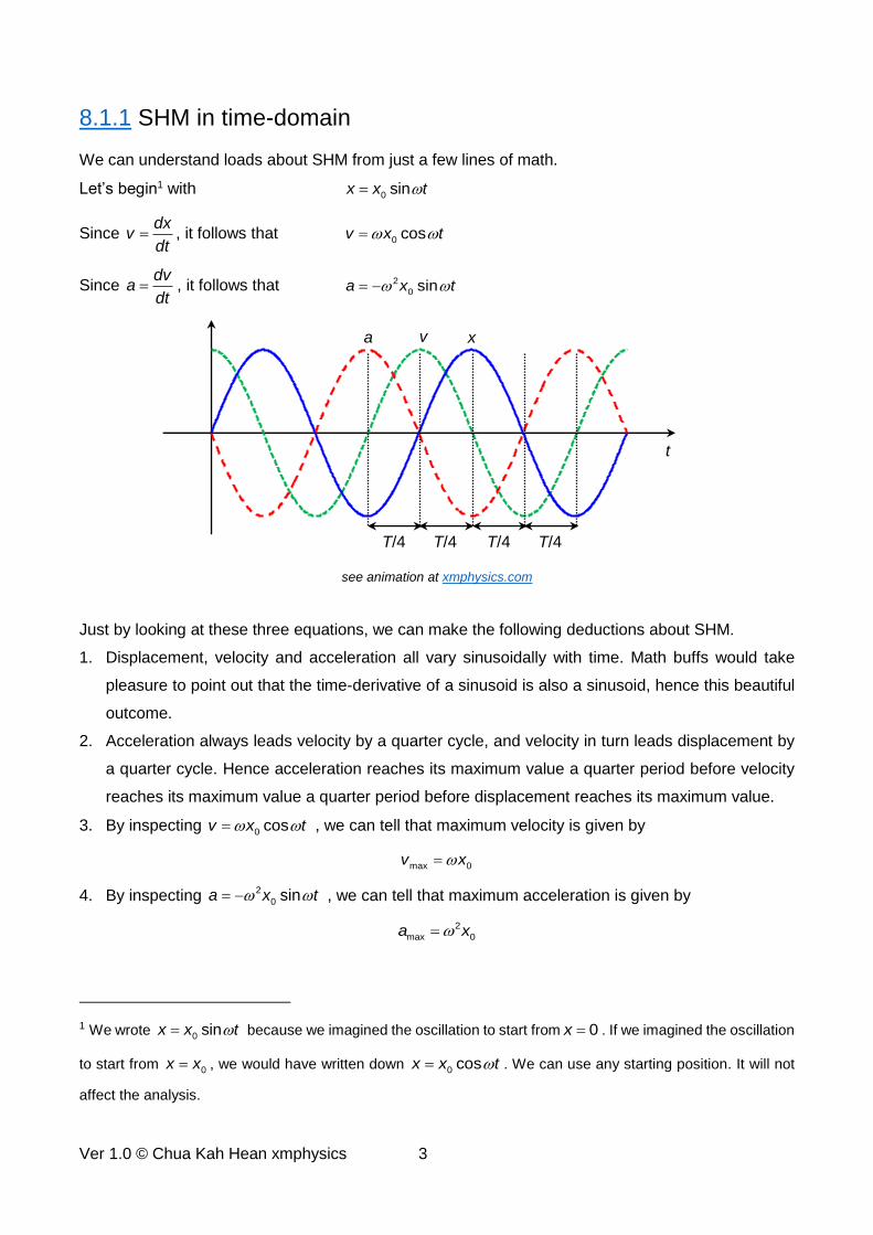
8.1.1 SHM in time-domain
We can understand loads about SHM from just a few lines of math.
Let’s begin1 with 0 sinx x t
Since dx
vdt
, it follows that 0 cosv x t
Since dv
adt
, it follows that 2
0 sina x t
see animation at xmphysics.com
Just by looking at these three equations, we can make the following deductions about SHM.
1. Displacement, velocity and acceleration all vary sinusoidally with time. Math buffs would take
pleasure to point out that the time-derivative of a sinusoid is also a sinusoid, hence this beautiful
outcome.
2. Acceleration always leads velocity by a quarter cycle, and velocity in turn leads displacement by
a quarter cycle. Hence acceleration reaches its maximum value a quarter period before velocity
reaches its maximum value a quarter period before displacement reaches its maximum value.
3. By inspecting 0 cosv x t , we can tell that maximum velocity is given by
max 0v x
4. By inspecting 2
0 sina x t , we can tell that maximum acceleration is given by
2
max 0a x
1 We wrote 0 sinx x t because we imagined the oscillation to start from 0x . If we imagined the oscillation
to start from 0x x , we would have written down 0 cosx x t . We can use any starting position. It will not
affect the analysis.
x a
t
T/4
v
T/4 T/4 T/4
Ver 1.0 © Chua Kah Hean xmphysics 4
8.1.2 SHM in the x-domain
In this section, we will obtain the a-x and v-x equations which we can use to calculate the acceleration
and velocity of a SHM at each displacement.
We begin by writing down the three time-domain equations.
0
0
2
0
sin
cos
sin
x x t
v x t
a x t
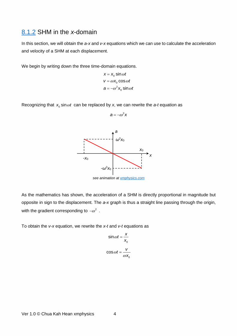
Recognizing that 0 sinx t can be replaced by x, we can rewrite the a-t equation as
2a x
see animation at xmphysics.com
As the mathematics has shown, the acceleration of a SHM is directly proportional in magnitude but
opposite in sign to the displacement. The a-x graph is thus a straight line passing through the origin,
with the gradient corresponding to 2 .
To obtain the v-x equation, we rewrite the x-t and v-t equations as
0
sinx
tx
0
cosv
tx
x0
-x0 x
a
-ω2x0
ω2x0

Ver 1.0 © Chua Kah Hean xmphysics 5
Using the trigonometic identity 2 2sin cos 1x x , we deftly get rid of the t terms.
2 2
2 2
0 0
2 2 2 2 2
0
2 2
0
sin cos 1
( ) ( ) 1
t t
x v
x x
x v x
v x x
Mathematics aficionados would recognize the first line as the equation of an ellipse, with intercepts at
0x x and 0v x .
see animation at xmphysics.com
Note also that the oscillation progresses in the clockwise direction along the elliptical graph. This is
obvious if you realize that for the top half of the graph, the velocity is positive, so the displacement
should progress towards the right (to become more positive). Likewise, for the bottom half of the graph,
the velocity is negative, so the displacement should progress towards the left (to become more
negative).
+ωx0
-ωx0
-x0 +x
0
x
v
Ver 1.0 © Chua Kah Hean xmphysics 6
8.1.3 The Half-Amplitude Problems
watch video explanation at xmphysics.com
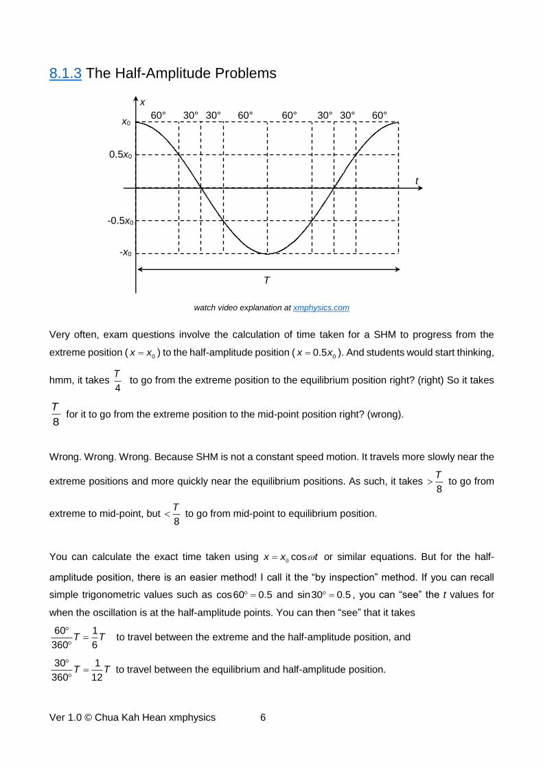
Very often, exam questions involve the calculation of time taken for a SHM to progress from the
extreme position ( 0x x ) to the half-amplitude position ( 00.5x x ). And students would start thinking,
hmm, it takes 4
T to go from the extreme position to the equilibrium position right? (right) So it takes
8
T for it to go from the extreme position to the mid-point position right? (wrong).
Wrong. Wrong. Wrong. Because SHM is not a constant speed motion. It travels more slowly near the
extreme positions and more quickly near the equilibrium positions. As such, it takes 8
T to go from
extreme to mid-point, but 8
T to go from mid-point to equilibrium position.
You can calculate the exact time taken using 0cosx x t or similar equations. But for the half-
amplitude position, there is an easier method! I call it the “by inspection” method. If you can recall
simple trigonometric values such as cos60 0.5 and sin30 0.5 , you can “see” the t values for
when the oscillation is at the half-amplitude points. You can then “see” that it takes
60 1
360 6T T
to travel between the extreme and the half-amplitude position, and
30 1
360 12T T
to travel between the equilibrium and half-amplitude position.
t
T
x
x0
-x0
-0.5x0
0.5x0
60° 30° 30° 60° 60° 30° 30° 60°

Ver 1.0 © Chua Kah Hean xmphysics 7
8.2 Restoring Force
Now that we have gone through the “kinematics” of SHM, let’s work out the “dynamics” behind SHM.
We begin by writing down the x-t, v-t and a-t equations for SHM.
0
0
2
0
sin
cos
sin
x x t
v x t
a x t
Since 0 sinx t is displacement x, we can rewrite acceleration as
2a x
If we multiply the mass of the oscillating body m to both sides, we get
2
netma F m x
From this equation, we attain the revelation that for a mass to undergo SHM, it must be experiencing
a net force that is (1) proportional to its displacement and (2) opposite in direction to its displacement.
Since the net force is always directed towards the equilibrium position, it is often called the restoring
force.
2
netF m x
x0
-x0 x
Fnet
-mω2x0
mω2x0

Ver 1.0 © Chua Kah Hean xmphysics 8
At this point you may be wondering, where on earth can we encounter a restoring force that varies
proportionately with displacement? Actually, such a restoring force is quite common. Take for example
the elastic force of a spring that obeys Hooke’s Law.
see animation at xmphysics.com
As illustrated in the diagram above, a mass is hung on a spring. In (b), the mass is at the equilibrium
position, where the downward weight mg is balanced by the upward tension force T of the spring. The
restoring force is zero at the equilibrium position.
In (c), the mass is displaced downward by x, so the spring is further extended by x. This results in the
tension increasing by kx, where k is the spring constant. Since T is larger than mg by kx, the restoring
force is kx and upward.
Similarly, in (d), the mass is displaced upward by x. Compared to the equilibrium position, the
extension is now shorter by x. This implies that T is smaller than mg by kx. The restoring force is thus
kx and downward.
In one equation
netF kx
That’s why when the mass is displaced from the equilibrium position and released, it goes into simple
harmonic motion. Neat.
equilibrium position
mg
(a)
T
Fnet
T
mg
T
mg
Fnet
x
unstretched
(b) (c) (d)
Ver 1.0 © Chua Kah Hean xmphysics 9
8.2.1 Natural Frequency
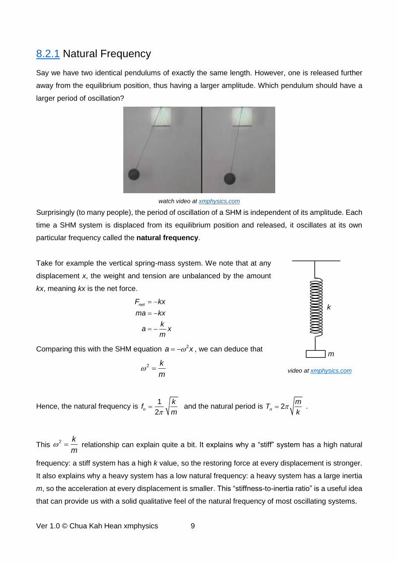
Say we have two identical pendulums of exactly the same length. However, one is released further
away from the equilibrium position, thus having a larger amplitude. Which pendulum should have a
larger period of oscillation?
watch video at xmphysics.com
Surprisingly (to many people), the period of oscillation of a SHM is independent of its amplitude. Each
time a SHM system is displaced from its equilibrium position and released, it oscillates at its own
particular frequency called the natural frequency.
Take for example the vertical spring-mass system. We note that at any
displacement x, the weight and tension are unbalanced by the amount
kx, meaning kx is the net force.
netF kx
ma kx
ka x
m
Comparing this with the SHM equation 2a x , we can deduce that
2 k
m
Hence, the natural frequency is 1
2n
kf
m and the natural period is 2n
mT
k .
This 2 k
m relationship can explain quite a bit. It explains why a “stiff” system has a high natural
frequency: a stiff system has a high k value, so the restoring force at every displacement is stronger.
It also explains why a heavy system has a low natural frequency: a heavy system has a large inertia
m, so the acceleration at every displacement is smaller. This “stiffness-to-inertia ratio” is a useful idea
that can provide us with a solid qualitative feel of the natural frequency of most oscillating systems.
m
k
video at xmphysics.com

Ver 1.0 © Chua Kah Hean xmphysics 10
Having said that, this “stiffness to inertia ratio” can be misleading when
applied to the pendulum. The mass of a pendulum does not affect its
natural frequency! Why? Because a larger mass results in both a
larger restoring force and a larger inertia. So the effect of a larger mass
cancels itself out (just like all object free fall at g regardless of mass).
However, the “stiffness” of a pendulum does depend on the
acceleration of free fall g, and its “inertia” does increase with length L.
The natural frequency of a pendulum thus turns out to be2 1
2n
gf
L .
Now that you understand the phenomenon of natural frequency, you will have a deeper satisfaction
watching these wonderfully intricate patterns (called Lissajous Figures) produced by two
simultaneous oscillations.
watch video at xmphysics.com
watch video at xmphysics.com
2 Be aware that this formula is valid only for small amplitude oscillations. Its derivation is not so straight forward
and is not required by the H2 syllabus.
L g
video at xmphysics.com

Ver 1.0 © Chua Kah Hean xmphysics 11
8.3 Energy of Oscillation
After we’re done with the kinematics and dynamics, it’s time to approach SHM from the energy
perspective.
An oscillation obviously has energy. Let’s begin by asking, where did this energy come from?
To produce an oscillation with amplitude x0, the system must first be displaced from its equilibrium
position to 0x x . This requires an external force to pull or push against the restoring force. The
work done by this external force corresponds to the (total) energy of oscillation, TE.
Recall that 2a x and the restoring force is 2
netF m x . Since the external force must match
the restoring force at every position, 2
extF m x at every position.
see animation at xmphysics.com
Since the area under the F-x graph is work done, we can derive the formula for TE to be
2 2 2
0 0 0
1 1( )( )
2 2TE x m x m x
-x0
x0
mω2x
0
-mω2x
0
x
Fext

Ver 1.0 © Chua Kah Hean xmphysics 12
During the oscillation, the restoring force does work continuously, resulting in continuous energy
conversion between kinetic energy KE and potential energy PE. From the principle of conservation of
energy, we know that at anytime and at anywhere,
TE KE PE
But at the extreme positions, KE is zero and PE is at its maximum. So
2 2
max 0
1
2PE TE m x .
Conversely, at the equilibrium position, PE is zero and KE is at its maximum. So
2 2
max 0
1
2KE TE m x
Just for fun, let’s write everything in one line
2 2
max max 0
1
2TE KE PE KE PE m x
Personally, I “memorise” this formula by remembering that max 0v x . So
2 2 2 2
max max max 0 0
1 1 1( )
2 2 2TE PE KE mv m x m x
Ver 1.0 © Chua Kah Hean xmphysics 13
8.3.1 SHM Energy in time-domain
Assuming that 0 cosv x t , we can write
2 2 2
0
1cos
2KE m x t
Since maxTE KE , we know
2 2
0
1
2TE m x
Since PE TE KE , we can work out that
2 2 2 2 2
0 0
2 2 2
0
2 2 2
0
1 1cos
2 2
1(1 cos )
2
1sin
2
PE m x m x t
m x t
m x t
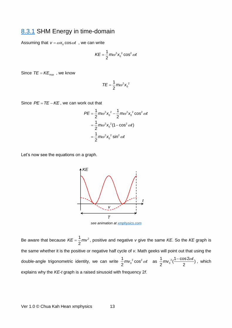
Let’s now see the equations on a graph.
see animation at xmphysics.com
Be aware that because 21
2KE mv , positive and negative v give the same KE. So the KE graph is
the same whether it is the positive or negative half cycle of v. Math geeks will point out that using the
double-angle trigonometric identity, we can write 2 2
0
1cos
2mv t as 2
0
1 1 cos2( )
2 2
tmv
, which
explains why the KE-t graph is a raised sinusoid with frequency 2f.
t
T
KE
v
Ver 1.0 © Chua Kah Hean xmphysics 14
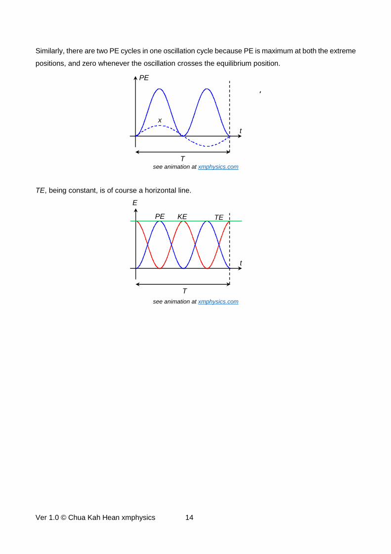
Similarly, there are two PE cycles in one oscillation cycle because PE is maximum at both the extreme
positions, and zero whenever the oscillation crosses the equilibrium position.
see animation at xmphysics.com
TE, being constant, is of course a horizontal line.
see animation at xmphysics.com
PE
t
T
x
PE KE
t
T
E
TE

Ver 1.0 © Chua Kah Hean xmphysics 15
8.3.2 SHM Energy in the x-domain
From 2 2
0v x x , we obtain
2 2 2
0
1( )
2KE m x x
Since maxTE KE at 0x ,
2 2
0
1
2TE m x
Since PE TE KE , we can work out
2 2 2 2 2
0 0
2 2
1 1( )
2 2
1
2
PE m x m x x
m x
A few things to note.
1. Both KE and PE are quadratic graphs and are mirror image of each other
2. The graphs intersect at 1
2E TE , 0
2
xx .
see animation at xmphysics.com
-x0 x
0
x
E
TE
KE
PE
Ver 1.0 © Chua Kah Hean xmphysics 16
8.4 Damped Oscillations
If an oscillation is completely undamped, the oscillation will go on forever. In
practice however, all oscillations must encounter some damping forces (e.g. air
resistance, friction). Damping saps the oscillation’s energy continuously, causing
its amplitude to decrease continuously over time.
see video at xmphysics.com
The behavior of damped oscillations has been studied extensively, in particular for the case of the
damping force being proportional to the velocity. It turns out that there are three distinct outcomes
depending on whether the oscillation experiences light damping, heavy damping or critical damping.
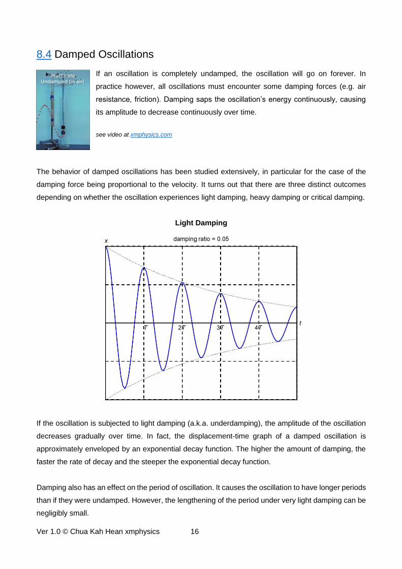
Light Damping
If the oscillation is subjected to light damping (a.k.a. underdamping), the amplitude of the oscillation
decreases gradually over time. In fact, the displacement-time graph of a damped oscillation is
approximately enveloped by an exponential decay function. The higher the amount of damping, the
faster the rate of decay and the steeper the exponential decay function.
Damping also has an effect on the period of oscillation. It causes the oscillation to have longer periods
than if they were undamped. However, the lengthening of the period under very light damping can be
negligibly small.

Ver 1.0 © Chua Kah Hean xmphysics 17
Heavy Damping
If the oscillation is subjected
to heavy damping (a.k.a.
overdamping), the oscillator
returns slowly to the
equilibrium position without
ever going past the
equilibrium position. In that
sense, heavy damping
totally stops the system from
oscillating.
Critical Damping
Critical damping is the
transition point between
light and heavy damping.
Critical damping sends a
displaced oscillator back to
the equilibrium position in
the shortest amount of time.
Because of this, critical
damping is the design
objective in many
engineering applications
(e.g. shock absorbers, car
suspension systems etc.).

Ver 1.0 © Chua Kah Hean xmphysics 18
This pictures below illustrate oscillations at different amounts of damping:
see images at xmphysics.com
For a real life demonstration, check out the following video:
watch video at xmphysics.com
Ver 1.0 © Chua Kah Hean xmphysics 19
8.4.1 Practical Applications of Damping
We actually encounter a lot of oscillatory systems in our daily lives. Some of these oscillations are
nuisances and should be damped and brought to rest quickly, before they drive us crazy.
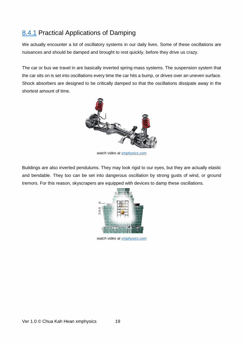
The car or bus we travel in are basically inverted spring-mass systems. The suspension system that
the car sits on is set into oscillations every time the car hits a bump, or drives over an uneven surface.
Shock absorbers are designed to be critically damped so that the oscillations dissipate away in the
shortest amount of time.
watch video at xmphysics.com
Buildings are also inverted pendulums. They may look rigid to our eyes, but they are actually elastic
and bendable. They too can be set into dangerous oscillation by strong gusts of wind, or ground
tremors. For this reason, skyscrapers are equipped with devices to damp these oscillations.
watch video at xmphysics.com

Ver 1.0 © Chua Kah Hean xmphysics 20
8.5 Forced Oscillation
Do you know that there are two ways to get an oscillation going?
The open and candid way is to displace the oscillator from its
equilibrium position and then release it. The oscillator will oscillate at
its natural frequency. This is called a free oscillation. The covert and
surreptitious way is to exert a small but continuous external periodic
driving force to the oscillator. In this case, the oscillator will be forced
to oscillate at the frequency of the driving force. This is called a
forced oscillation.
watch video at xmphysics.com
For a free oscillation, the energy is transferred to the oscillator in “one lump payment” at the beginning
when the oscillator was displaced. The amplitude of oscillation starts off at a maximum and decreases
gradually over time due to damping.
For a forced oscillation, however, energy is continuously transferred to the oscillator by the periodic
driving force. The amplitude of the forced oscillation starts at zero, and increases over time, and
stabilizes at a final amplitude when the rate of input of energy from the driver is matched by the rate
of loss of energy to the surrounding due to damping.
see animation at xmphysics.com
The efficacy of energy transfer from the driver to the oscillator is dependent on how close the driving
frequency is to the natural frequency of the oscillatory system. When there is a large mismatch, the
energy transfer from the driver to the oscillator is inefficient, and the forced oscillation will only attain
a low amplitude.
time
displacement Final amplitude of forced oscillation
Ver 1.0 © Chua Kah Hean xmphysics 21
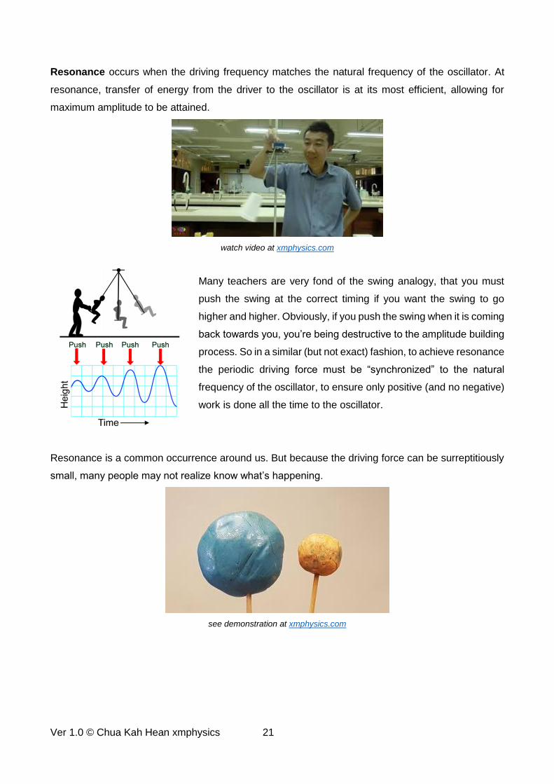
Resonance occurs when the driving frequency matches the natural frequency of the oscillator. At
resonance, transfer of energy from the driver to the oscillator is at its most efficient, allowing for
maximum amplitude to be attained.
watch video at xmphysics.com
Many teachers are very fond of the swing analogy, that you must
push the swing at the correct timing if you want the swing to go
higher and higher. Obviously, if you push the swing when it is coming
back towards you, you’re being destructive to the amplitude building
process. So in a similar (but not exact) fashion, to achieve resonance
the periodic driving force must be “synchronized” to the natural
frequency of the oscillator, to ensure only positive (and no negative)
work is done all the time to the oscillator.
Resonance is a common occurrence around us. But because the driving force can be surreptitiously
small, many people may not realize know what’s happening.
see demonstration at xmphysics.com

Ver 1.0 © Chua Kah Hean xmphysics 22
8.5.1 Resonance Curve
Consider an oscillatory system with natural frequency f0. Let’s couple this
system to a driver of varying frequency f but fixed amplitude A0. If we plot
on a graph how the amplitude of the forced oscillation A varies with the
driver’s frequency f, we obtain the so-called resonance curve.
see applet at xmphysics.com
The main features of the resonance curve are:
1. Amplitude A peaks at 0f f .
When the driver is driving at the natural frequency of the oscillator, it’s like a match made in heaven.
The energy transfer from the driver to the oscillator is at its most efficient. In fact, the oscillator is
able to accumulate the energy transferred and reaches a maximum amplitude that is many times
larger than the amplitude of the driver.
2. As f approaches 0, A approaches A0.
Put it this way. When a slow driver meets a quick oscillator, the oscillator is so “nimble” it tracks
the motion of the driver exactly. So the oscillator has the same amplitude of oscillation as the
driver.
3. As f approaches infinity, A approaches zero.
When a quick driver meets a slow oscillator, the oscillator is so “retarded” it simply cannot respond
in time. The driving forces changes too rapidly for the oscillator and its amplitude is stuck at zero.
A
f
f0
A0
driver
oscillator
A0
A
f

Ver 1.0 © Chua Kah Hean xmphysics 23
8.5.2 Effect of Damping on Resonance
Resonance can be a nuisance at times. In such situations, damping forces are actually very desirable.
Remember that in a forced oscillation, the final amplitude reached is the amplitude at which the rate
of gain of energy (from the driver) is matched by the rate of loss of energy (to the surrounding). With
higher damping, the rate of energy loss at each amplitude is higher. This results in a lower resonance
amplitude.
watch video at xmphysics.com
Now let’s look at the effect of damping on our resonance curves.
see applet at xmphysics.com
0
5
10
15
20
25
30
35
40
45
50
0 0.5 1 1.5 2
Damping Ratio:
--- 0.01
--- 0.05
--- 0.10
A
A0
f f0

Ver 1.0 © Chua Kah Hean xmphysics 24
Notice that whenever damping is increased, the entire resonance curve is lower not just at the
resonance frequency, but at every frequency (except 0f ). On the other hand, decreased damping
lowers the rate of energy loss to resistive forces, and results in a higher resonance curve. In theory,
at zero damping, the resonance amplitude should reach infinity. In practice, however, there are
physical constraints. For examples, a pendulum cannot swing more than 90°, a spring cannot be
compressed to zero length, or the oscillator cannot withstand the physical stress and breaks down
when the oscillation is too vigorous.
Do you remember that damping lengthens the period of oscillation? Similarly, damping causes
resonance to occur at a frequency slightly lower than the oscillator’s natural frequency. So the
resonance peaks will shift towards lower frequency as damping increases. But again, the shift is not
significant at very light damping conditions.
0
1
2
3
4
5
6
0 0.5 1 1.5 2 2.5 3
Damping Ratio:
--- 0.05
--- 0.10
--- 0.25
--- 0.50
--- 0.75
A A0
f f0
Ver 1.0 © Chua Kah Hean xmphysics 25
8.A Angular Frequency vs Angular Velocity
The angular frequency is a rather abstract concept which deserves some discussion.
22 f
T
At the most basic level, from 2 f , you should appreciate that the angular frequency ω is simply
the frequency of the oscillation multiplied by 2 .
At a more abstract level, from 0 sinx x t , we can
think of t as the phase angle of the oscillation.
So ω is the “velocity” at which the phase of the
oscillation progresses. Watch this demonstration
where 17 pendulums with different ω are put to a
race.
see applet at xmphysics.com
The angular frequency ω in SHM is actually very similar in concept to the angular velocity ω in circular
motion. (This explains why they are both given the symbol ω.)
For oscillations, 2d
dt T
is the rate of change of phase angle.
For circular motion, 2d
dt T
is the rate of change of angular displacement.
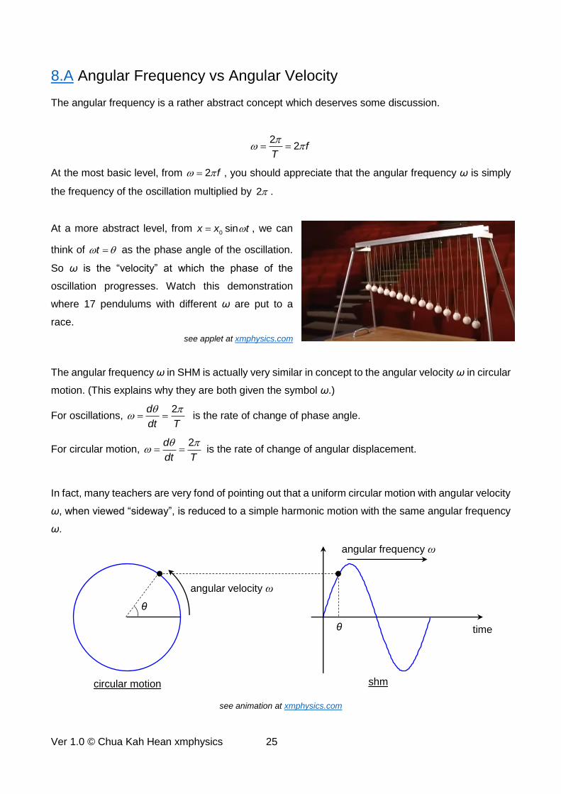
In fact, many teachers are very fond of pointing out that a uniform circular motion with angular velocity
ω, when viewed “sideway”, is reduced to a simple harmonic motion with the same angular frequency
ω.
see animation at xmphysics.com
θ
θ
angular velocity ω
angular frequency ω
time
circular motion shm

Ver 1.0 © Chua Kah Hean xmphysics 26
8.B More Demonstrations
These demonstrations are arguably beyond the H2 syllabus. Nevertheless, they are fun and they may
help you understand the H2 syllabus.
watch videos at xmphysics.com
Barton’s Pendulum
The Coupled Pendulum
Tuning Fork Resonance
The Coupled Inverted Pendulum
Recommended