Embed Size (px)
Citation preview
8/12/2019 Introduction to Oscillation
http://slidepdf.com/reader/full/introduction-to-oscillation 1/37
BSC 417/517
Environmental Modeling
Introduction to Oscillations
8/12/2019 Introduction to Oscillation
http://slidepdf.com/reader/full/introduction-to-oscillation 2/37
Oscillations are Common
• Oscillatory behavior is common in all types
of natural (physical, chemical, biological)
and human (engineering, industry,economic) systems
• Systems dynamics modeling is a powerful
tool to help understand the basis for andinfluence of oscillations on environmental
systems
8/12/2019 Introduction to Oscillation
http://slidepdf.com/reader/full/introduction-to-oscillation 3/37
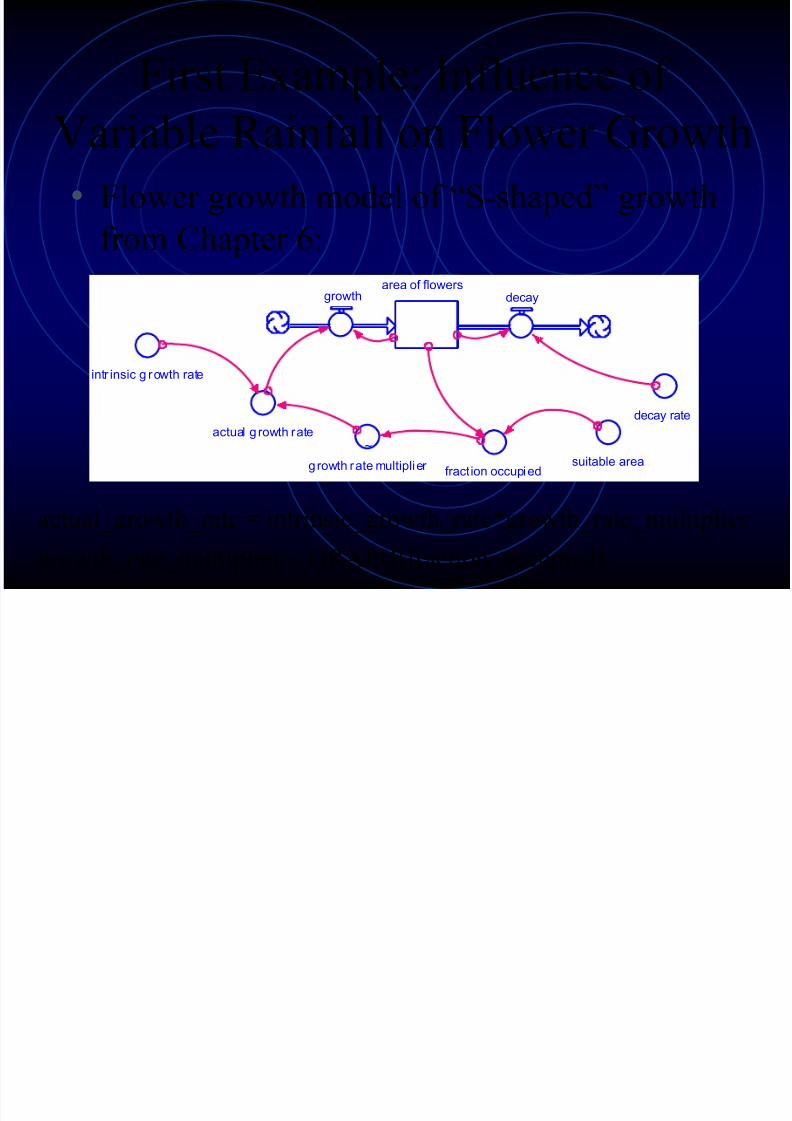
First Example: Influence of
Variable Rainfall on Flower Growth• Flower growth model of “S-shaped” growth
from Chapter 6:area of flowers
growth decay
decay rateactual g rowth rate
intr insic g rowth rate
fraction occupied
~
growth rate multiplier suitable area
actual_growth_rate = intrinsic_growth_rate*growth_rate_multiplier
growth_rate_multiplier = GRAPH(fraction_occupied)
8/12/2019 Introduction to Oscillation
http://slidepdf.com/reader/full/introduction-to-oscillation 4/37
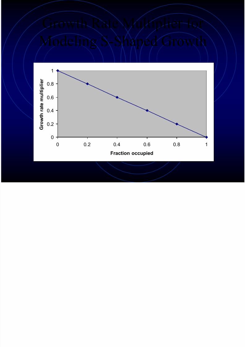
Growth Rate Multiplier for
Modeling S-Shaped Growth
0
0.2
0.4
0.6
0.8
1
0 0.2 0.4 0.6 0.8 1
Fraction occupied
G
r o w t h r a t e m u l t i p l i e r
8/12/2019 Introduction to Oscillation
http://slidepdf.com/reader/full/introduction-to-oscillation 5/37
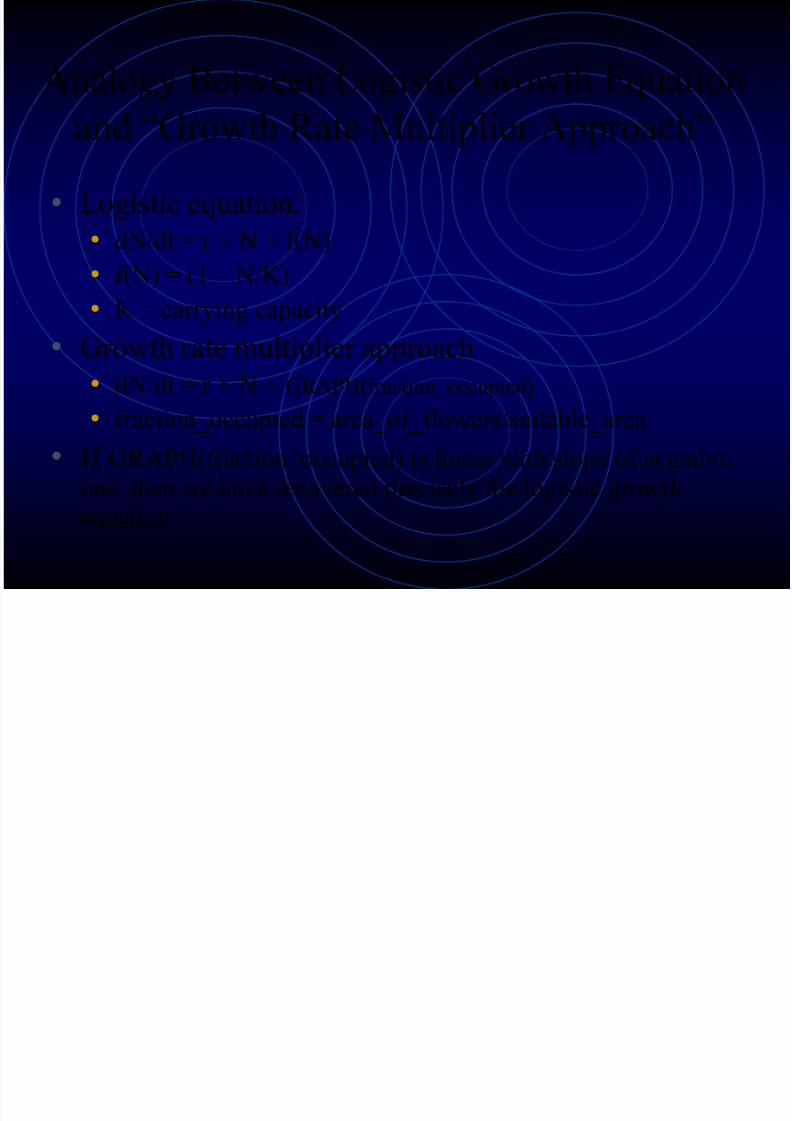
Analogy Between Logistic Growth Equation
and “Growth Rate Multiplier Approach”
• Logistic equation:
• dN/dt = r × N × f(N)
• f(N) = (1 – N/K)• K = carrying capacity
• Growth rate multiplier approach
• dN/dt = r × N × GRAPH(fraction_occupied)
• fraction_occupied = area_of_flowers/suitable_area
• If GRAPH(fraction_occupied) is linear with slope of negativeone, then we have recovered precisely the logistic growthequation
8/12/2019 Introduction to Oscillation
http://slidepdf.com/reader/full/introduction-to-oscillation 6/37
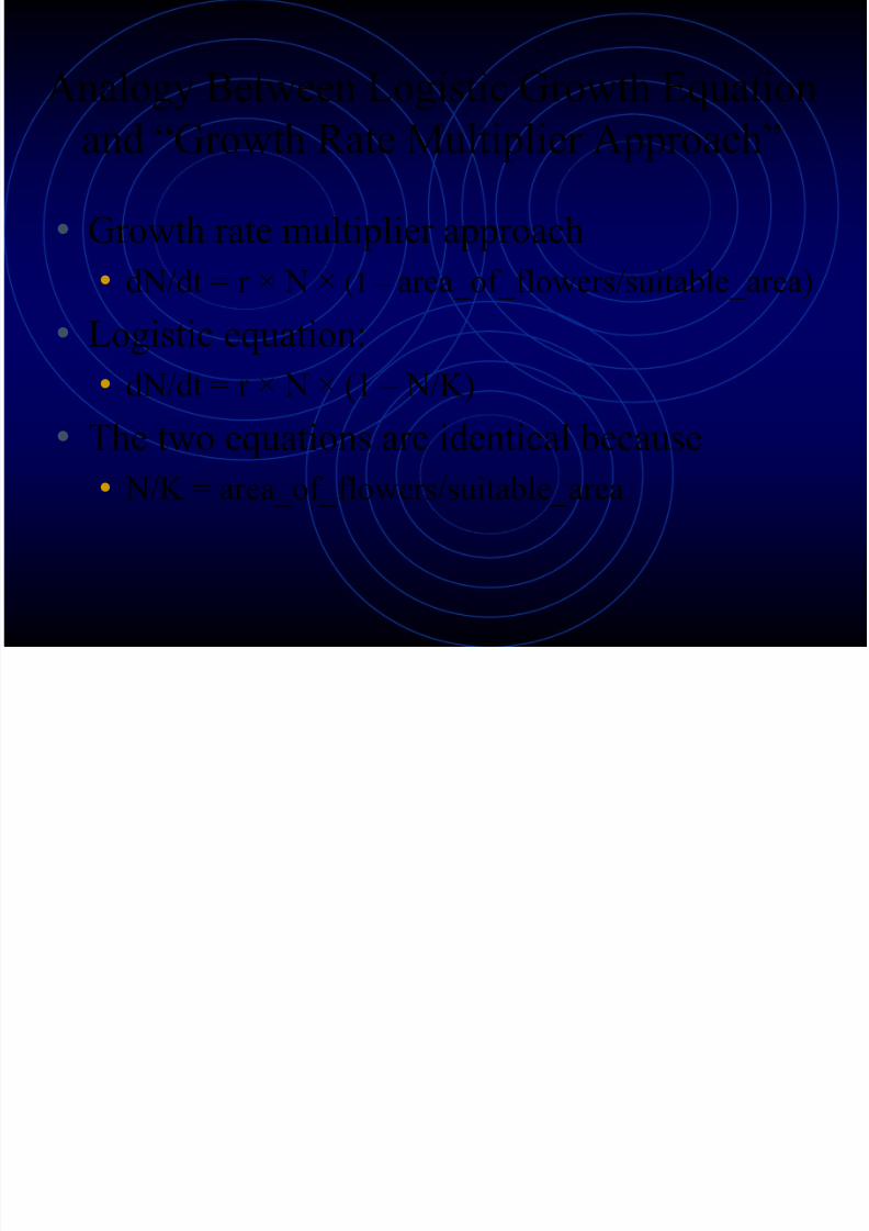
Analogy Between Logistic Growth Equation
and “Growth Rate Multiplier Approach”
• Growth rate multiplier approach
• dN/dt = r × N × (1 – area_of_flowers/suitable_area)
• Logistic equation:
• dN/dt = r × N × (1 – N/K)
• The two equations are identical because• N/K = area_of_flowers/suitable_area
8/12/2019 Introduction to Oscillation
http://slidepdf.com/reader/full/introduction-to-oscillation 7/37
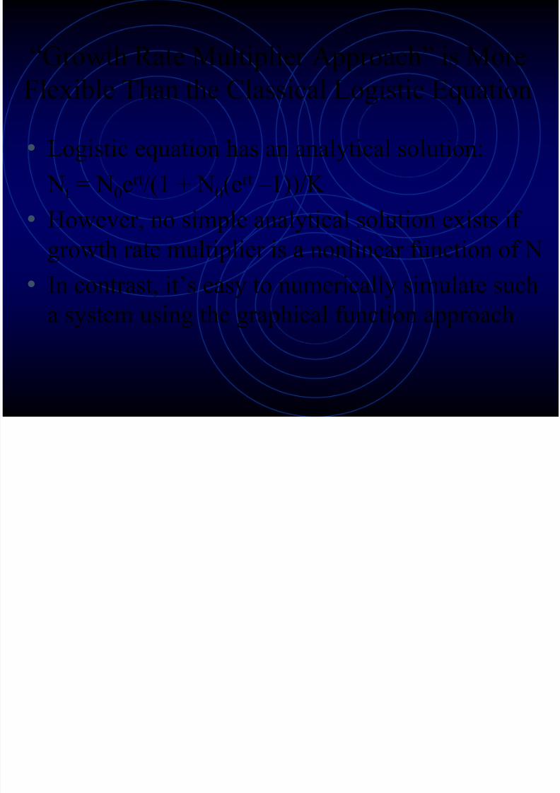
“Growth Rate Multiplier Approach” is More
Flexible Than the Classical Logistic Equation
• Logistic equation has an analytical solution:
Nt = N0e
rt
/(1 + N0(e
rt
– 1))/K• However, no simple analytical solution exists if
growth rate multiplier is a nonlinear function of N
• In contrast, it’s easy to numerically simulate sucha system using the graphical function approach

8/12/2019 Introduction to Oscillation
http://slidepdf.com/reader/full/introduction-to-oscillation 8/37
“Growth Rate Multiplier Approach” is More
Flexible Than the Classical Logistic Equation
0
0.2
0.4
0.6
0.8
1
0 0.2 0.4 0.6 0.8 1
Fraction occupied
G
r o w t h r a t e m u l t i p l i e r
8/12/2019 Introduction to Oscillation
http://slidepdf.com/reader/full/introduction-to-oscillation 9/37
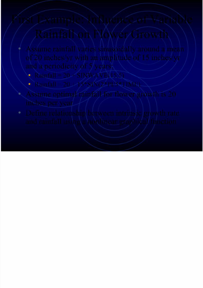
First Example: Influence of Variable
Rainfall on Flower Growth• Assume rainfall varies sinusoidally around a mean
of 20 inches/yr with an amplitude of 15 inches/yrand a periodicity of 5 years:
• Rainfall = 20 + SINWAVE(15,5)
• Rainfall = 20 + 15*SIN(2*PI/5*TIME)
• Assume optimal rainfall for flower growth is 20
inches per year• Define relationship between intrinsic growth rateand rainfall using a nonlinear graphical function

8/12/2019 Introduction to Oscillation
http://slidepdf.com/reader/full/introduction-to-oscillation 10/37
Relationship Between Intrinsic
Growth Rate and Rainfall
0
0.2
0.4
0.6
0.8
1
0 5 10 15 20 25 30 35 40
Rainfall (inches/year)
I n t r i n s i c e g r o w t h r a t e ( 1 / y r )
8/12/2019 Introduction to Oscillation
http://slidepdf.com/reader/full/introduction-to-oscillation 11/37
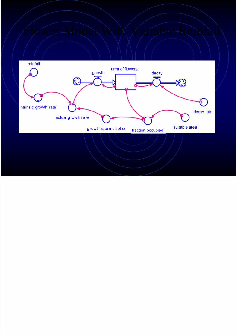
Flower Model With Variable Rainfall
area of flowersgrowth decay
decay rate
actual growth rate
~
intrinsic growth rate
fraction occupied~
growth rate multiplier suitable area
rainfall
8/12/2019 Introduction to Oscillation
http://slidepdf.com/reader/full/introduction-to-oscillation 12/37
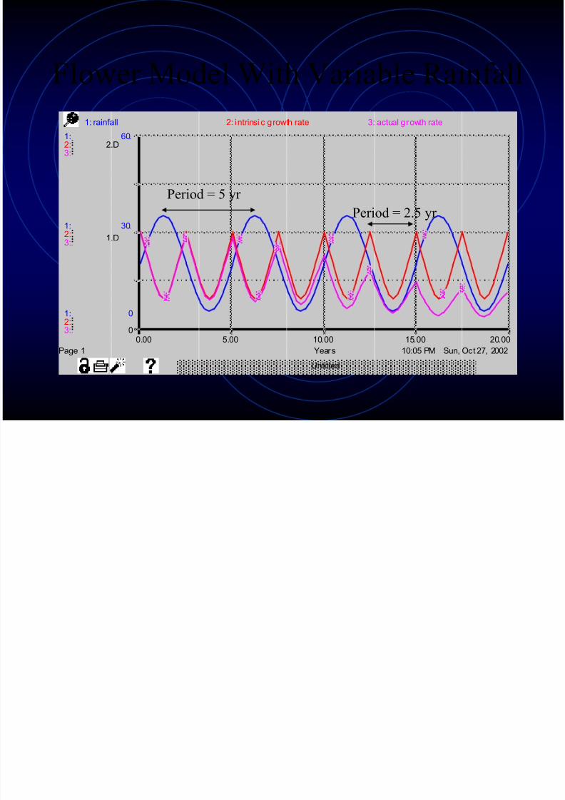
Flower Model With Variable Rainfall
10:05 PM Sun, Oct 27, 2002
Untitled
Page 1
0.00 5.00 10.00 15.00 20.00
Years
1:
1:
1:
2:
2:
2:
3:
3:
3:
0
30.
60.
0
1.D
2.D
1: rainfall 2: intrinsi c growth rate 3: actual growth rate
1 1 1 1
2 2 2 2
33
3
3
Period = 5 yrPeriod = 2.5 yr

8/12/2019 Introduction to Oscillation
http://slidepdf.com/reader/full/introduction-to-oscillation 13/37
Flower Model With Variable Rainfall
10:10 PM Sun, Oct 27, 2002
Untitled
Page 1
0.00 10.00 20.00 30.00 40.00
Years
1:
1:
1:
2:
2:
2:
3:
3:
3:
0
350
700
0
100
200
0
150
300
1: area of flowers 2: decay 3: growth
1
1
1 1
2
2
2 2
3
3 3 3
8/12/2019 Introduction to Oscillation
http://slidepdf.com/reader/full/introduction-to-oscillation 14/37
Flower Model With Variable Rainfall
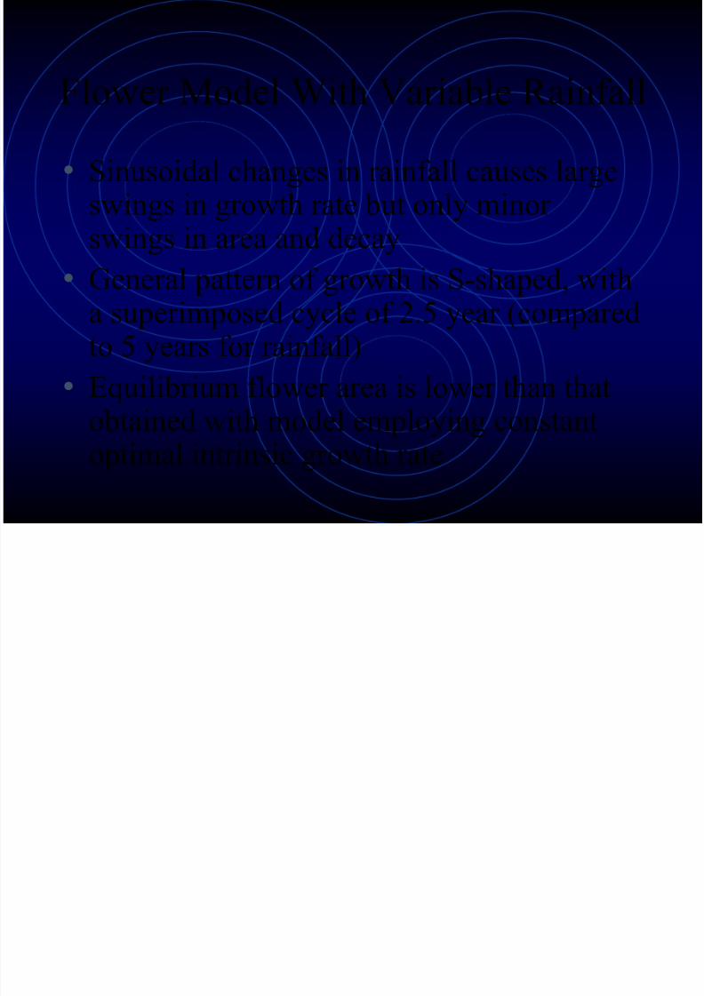
• Sinusoidal changes in rainfall causes largeswings in growth rate but only minor
swings in area and decay• General pattern of growth is S-shaped, with
a superimposed cycle of 2.5 year (comparedto 5 years for rainfall)
• Equilibrium flower area is lower than thatobtained with model employing constantoptimal intrinsic growth rate

8/12/2019 Introduction to Oscillation
http://slidepdf.com/reader/full/introduction-to-oscillation 15/37
General Conclusions
• Cycles imposed from outside the system
can be transformed as their affects “pass
through” the system • Periodicity can be modified as a result of
system dynamics
• Quantitative effect of external variationscan be moderated at the stocks in the system
8/12/2019 Introduction to Oscillation
http://slidepdf.com/reader/full/introduction-to-oscillation 16/37
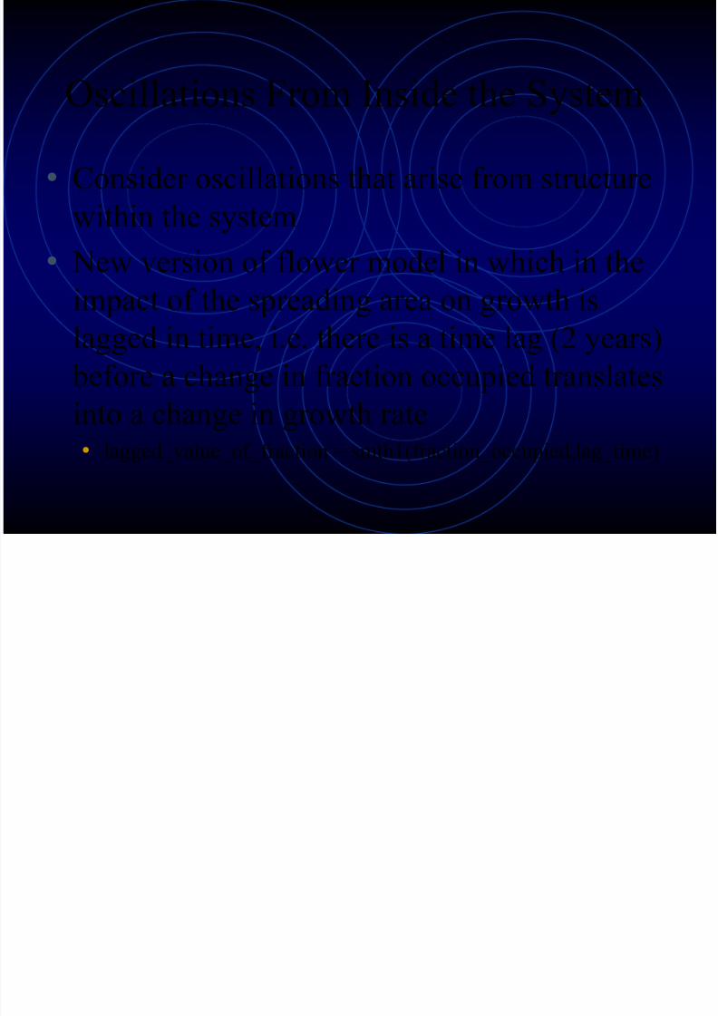
Oscillations From Inside the System
• Consider oscillations that arise from structure
within the system
• New version of flower model in which in theimpact of the spreading area on growth is
lagged in time, i.e. there is a time lag (2 years)
before a change in fraction occupied translatesinto a change in growth rate• lagged_value_of_fraction = smth1(fraction_occupied,lag_time)
8/12/2019 Introduction to Oscillation
http://slidepdf.com/reader/full/introduction-to-oscillation 17/37
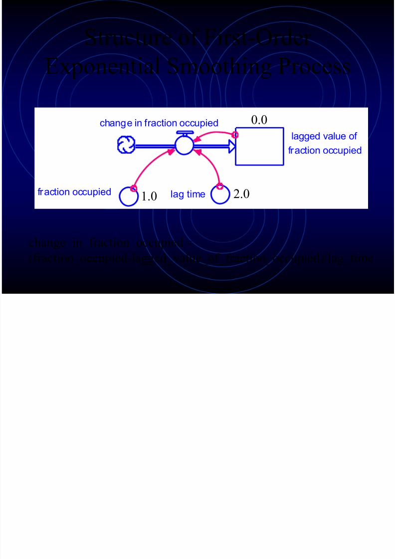
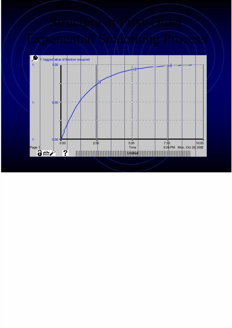
Structure of First-Order
Exponential Smoothing Process
lagged value offraction occupied
change in fraction occupied
fraction occupied lag time
change_in_fraction_occupied =
(fraction_occupied-lagged_value_of_fraction_occupied)/lag_time
1.0 2.0
0.0
8/12/2019 Introduction to Oscillation
http://slidepdf.com/reader/full/introduction-to-oscillation 18/37
Structure of First-Order
Exponential Smoothing Process
9:26 PM Mon, Oct 28, 2002
Untitled
Page 1
0.00 2.50 5.00 7.50 10.00
Time
1:
1:
1:
0.00
0.50
1.00
1: lagged value of fraction occupied
1
1
11
8/12/2019 Introduction to Oscillation
http://slidepdf.com/reader/full/introduction-to-oscillation 19/37
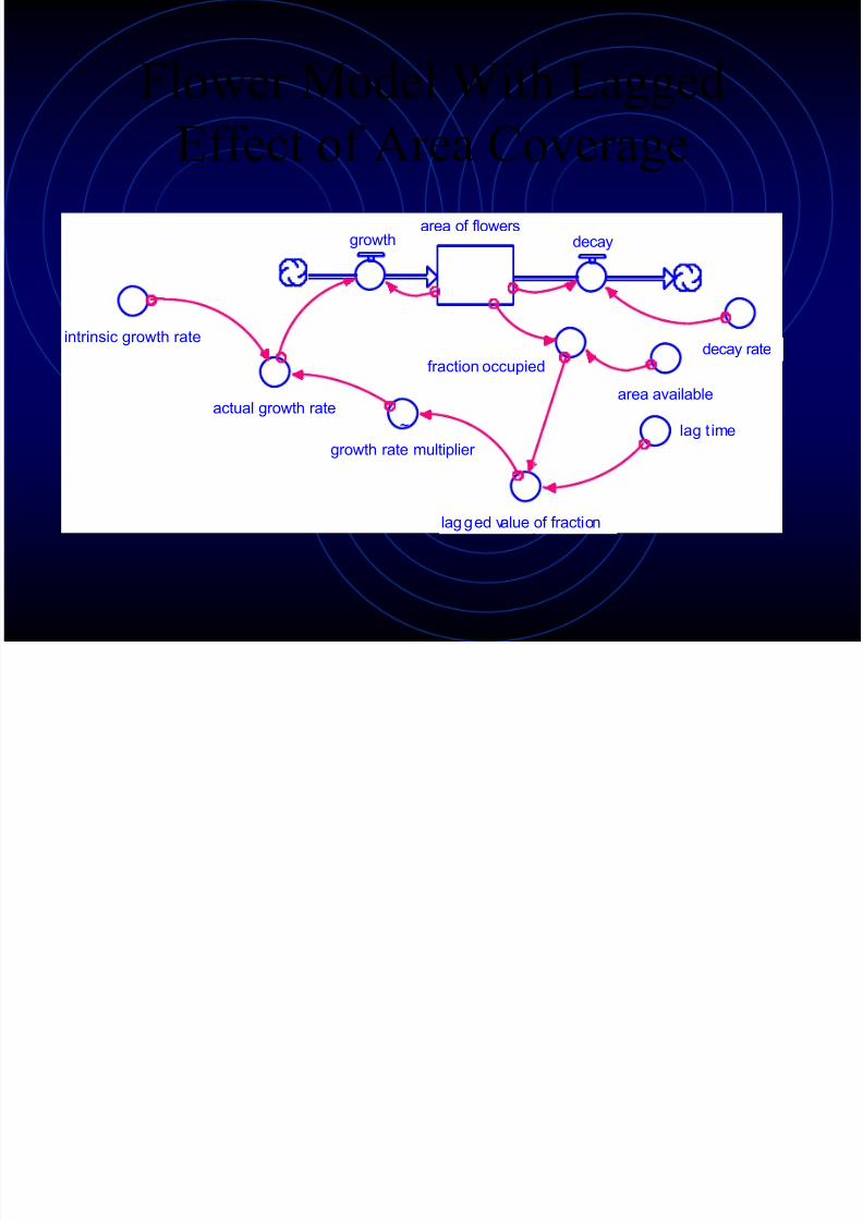
Flower Model With Lagged
Effect of Area Coveragearea of flowers
growth decay
decay rate
actual growth rate
intrinsic growth rate
fraction occupied
~
growth rate multiplier
area available
lagged value of fraction
lag t ime
8/12/2019 Introduction to Oscillation
http://slidepdf.com/reader/full/introduction-to-oscillation 20/37
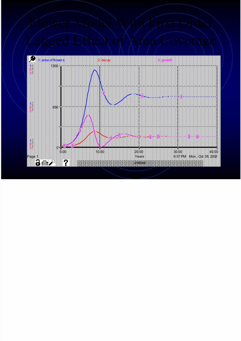
Flower Model With First Order
Lagged Effect of Area Coverage
9:37 PM Mon, Oct 28, 2002
Untitled
Page 1
0.00 10.00 20.00 30.00 40.00
Years
1:
1:
1:
2:
2:
2:
3:
3:
3:
0
650
1300
1: area of flowers 2: decay 3: growth
1
11 1
2
2 2 2
3
3 3 3
8/12/2019 Introduction to Oscillation
http://slidepdf.com/reader/full/introduction-to-oscillation 21/37
Flower Model With First Order
Lagged Effect of Area Coverage• Area of flowers overshoots maximum
available area, which causes a major decline
in growth so that decay exceeds growth by 8th
year of simulation
• Area declines, which frees up space, whicheventually results in an increase in growth
• Variations in growth and decay eventuallyfade away as the system approaches dynamicequilibrium = “damped oscillation”
8/12/2019 Introduction to Oscillation
http://slidepdf.com/reader/full/introduction-to-oscillation 22/37
Higher Order Lags are Possible
• STELLA has built-in function for 1st, 3rd,
and nth order smoothing, which can be used
to produced any desired order of lag• The higher the order of the lag, the longer
the delay in impact
• Example = third order lag
8/12/2019 Introduction to Oscillation
http://slidepdf.com/reader/full/introduction-to-oscillation 23/37
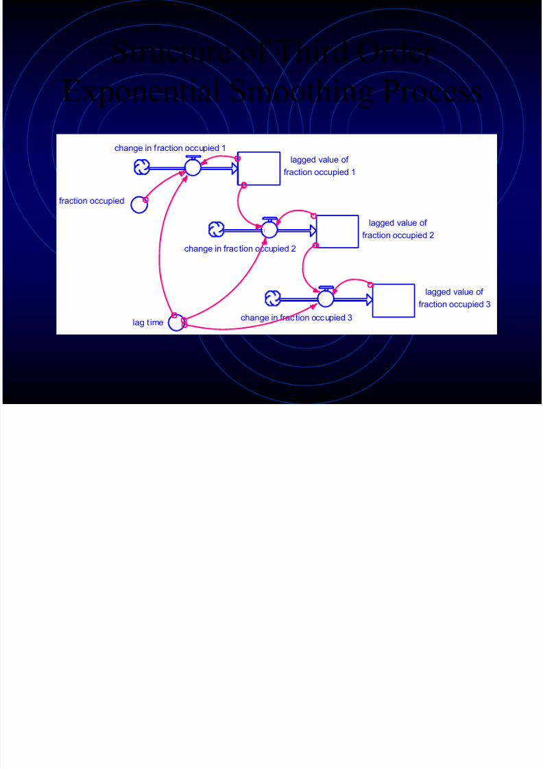
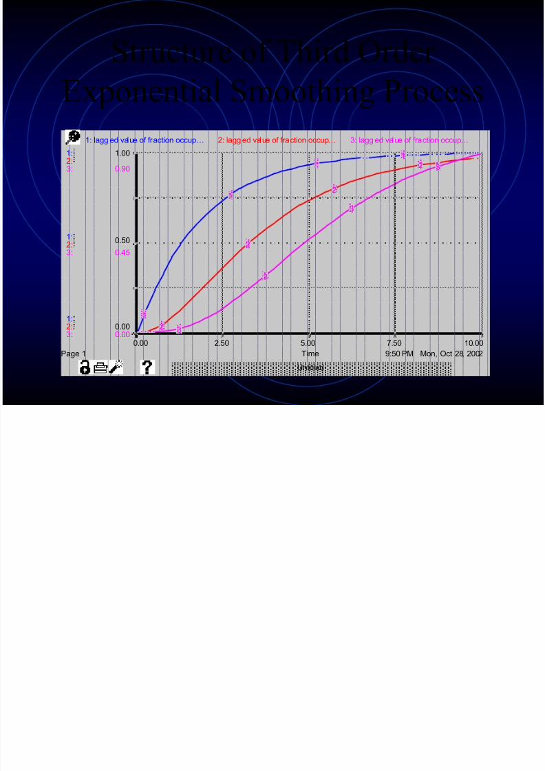
Structure of Third Order
Exponential Smoothing Process
lagged value of
fraction occupied 1
change in fraction occupied 1
fraction occupied
lag t ime
lagged value of
fraction occupied 2
change in frac tion occupied 2
lagged value of
fraction occupied 3
change in frac tion occupied 3
8/12/2019 Introduction to Oscillation
http://slidepdf.com/reader/full/introduction-to-oscillation 24/37
Structure of Third Order
Exponential Smoothing Process
9:50 PM Mon, Oct 28, 2002
Untitled
Page 1
0.00 2.50 5.00 7.50 10.00
Time
1:
1:
1:
2:
2:
2:
3:
3:
3:
0.00
0.50
1.00
0.00
0.45
0.90
1: lagg ed value of fraction occup… 2: lagg ed value of fraction occup… 3: lagg ed value of fraction occup…
1
1
11
2
2
2
2
3
3
3
3

8/12/2019 Introduction to Oscillation
http://slidepdf.com/reader/full/introduction-to-oscillation 25/37
Flower Model With First vs. Third Order
Lagged Effect of Area Coverage
9:54 PM Mon, Oct 28, 2002
Untitled
Page 1
0.00 10.00 20.00 30.00 40.00
Years
1:
1:
1:
2:
2:
2:
0
750
1500
1: area of flowers fir rst order l ag 2: area of flowers third order lag
1
11 1
2
2 2
2

8/12/2019 Introduction to Oscillation
http://slidepdf.com/reader/full/introduction-to-oscillation 26/37
Flower Model With First vs. Third Order
Lagged Effect of Area Coverage• Third order lag shows more volatility
• Flower area shoots farther past the carrying
capacity of 1000 acres and goes throughlarge oscillations before dynamicequilibrium is achieved
• Increased volatility arises because of thelonger lag implicit in the third ordersmoothing
8/12/2019 Introduction to Oscillation
http://slidepdf.com/reader/full/introduction-to-oscillation 27/37
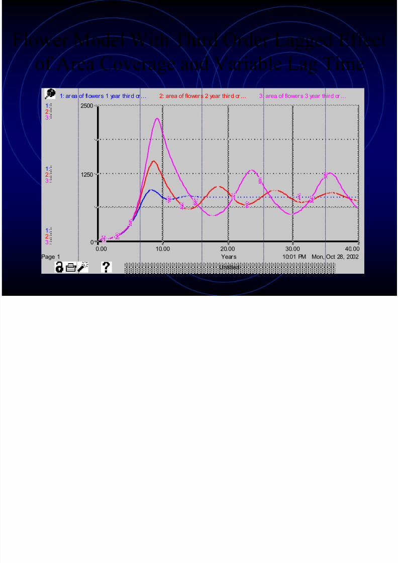
Further Examination of Lag Time Effect
• Compare simulations with third order
smoothing and lag times of 1, 2, or 3 years
• Longer lags lead to greater volatility
• Flower area in simulation with 3 year lag
time shoots up to greater than 2X the
carrying capacity
8/12/2019 Introduction to Oscillation
http://slidepdf.com/reader/full/introduction-to-oscillation 28/37
Flower Model With Third Order Lagged Effect
of Area Coverage and Variable Lag Time
10:01 PM Mon, Oct 28, 2002
Untitled
Page 1
0.00 10.00 20.00 30.00 40.00
Years
1:
1:
1:
2:
2:
2:
3:
3:
3:
0
1250
2500
1: area of flowers 1 year third or… 2: area of flowers 2 year third or… 3: area of flowers 3 year third or…
1
1 1 1
2
2 22
3
3
33

8/12/2019 Introduction to Oscillation
http://slidepdf.com/reader/full/introduction-to-oscillation 29/37
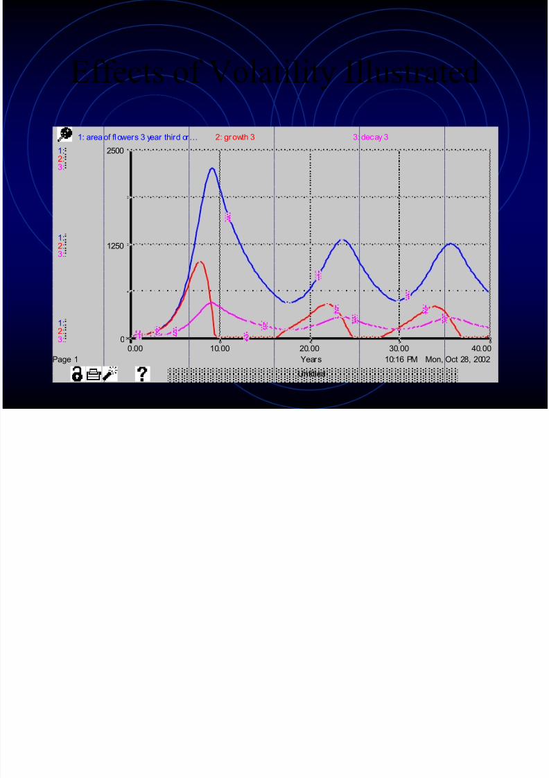
Effects of Volatility Illustrated
• Plot growth and decay together with flower area for simulationwith 3 year time lag
• Flower area and growth rate increase in parallel even aftercarrying capacity is reached; flowers do not “feel” the effect ofspace limitation due to the time lag
• Once effect of space limitation kicks in, growth rate dropsrapidly to zero
• Active growth does not resume until ca. year 15, meanwhile
decay continues on• New growth spurt occurs at around year 20, utilizing space
freed-up during previous period of decline
• Magnitude of oscillations does not decline over time =“sustained oscillation”
8/12/2019 Introduction to Oscillation
http://slidepdf.com/reader/full/introduction-to-oscillation 30/37
Effects of Volatility Illustrated
10:16 PM Mon, Oct 28, 2002
Untitled
Page 1
0.00 10.00 20.00 30.00 40.00
Years
1:
1:
1:
2:
2:
2:
3:
3:
3:
0
1250
2500
1: area of flowers 3 year third or… 2: growth 3 3: decay 3
1
1
1
1
22
2 2
33
3 3
8/12/2019 Introduction to Oscillation
http://slidepdf.com/reader/full/introduction-to-oscillation 31/37
Effects of Volatility Illustrated
• Key reason for sustained volatility of the model withlong time lag is the high intrinsic growth rate
• To illustrate, repeat simulation with different values of
the intrinsic growth rate and a 2 year lag time • Sustained oscillation (volatility) occurs with intrinsic
growth rate of 1.5/yr
• With intrinsic growth rate of 1.0/yr, oscillationsdampen over time
• With intrinsic growth rate of 0.5/yr, no oscillationsoccur (system is “overdamped”)

8/12/2019 Introduction to Oscillation
http://slidepdf.com/reader/full/introduction-to-oscillation 32/37
Influence of Intrinsic Growth
Rate on Volatility
10:28 PM Mon, Oct 28, 2002
Untitled
Page 1
0.00 10.00 20.00 30.00 40.00
Years
1:
1:
1:
0
1500
3000
area of flowers 2 year third order lag 2: 1 - 2 - 3 -
1
1
1 1
2
2 2 2
3
3
3
3
r = 1.5/yr
r = 1.0/yr
r = 0.5/yr
8/12/2019 Introduction to Oscillation
http://slidepdf.com/reader/full/introduction-to-oscillation 33/37
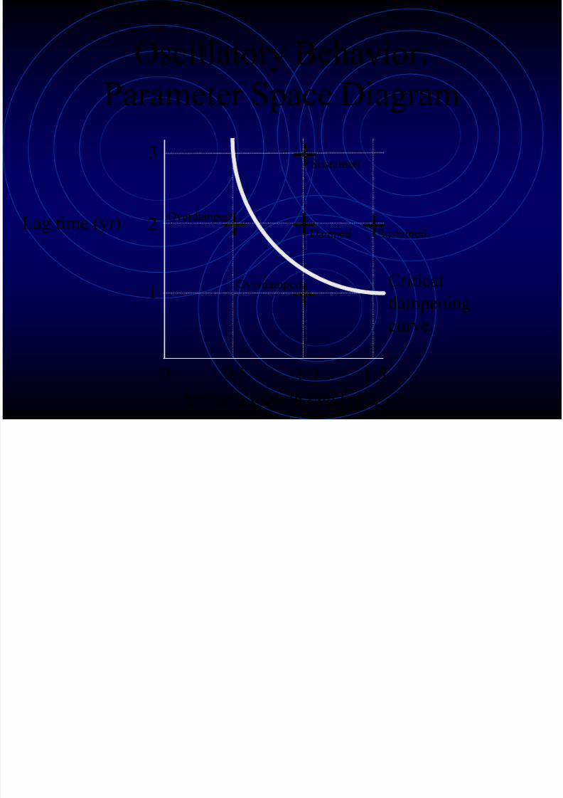
Summary of Oscillatory Tendencies
• Simple flower model gives rise to three basic patterns of oscillatory behavior:
• Overdamped• Damped
• Sustained
depending on the values for lag time andintrinsic growth rate
• Can summarize the observed effects with a parameter space diagram
8/12/2019 Introduction to Oscillation
http://slidepdf.com/reader/full/introduction-to-oscillation 34/37
Oscillatory Behavior:
Parameter Space Diagram
+
+
+ +
+
0 0.5 1.0 1.5
Intrinsic growth rate (yr -1)
Lag time (yr)
1
2
3
Overdamped
Overdamped
Sustained
SustainedDamped
Critical
dampeningcurve
8/12/2019 Introduction to Oscillation
http://slidepdf.com/reader/full/introduction-to-oscillation 35/37
Critical Dampening Curve• Hastings (1997) analyzed a logistic growth model
with lags, and found that oscillations occurred onlywhen the product of the intrinsic growth rate and timelag (a dimensionless parameter ) was greater than 1.57
• Flower model is not identical to Hastings’s model, but there is sufficient similarity to warrant using hisfindings as a working hypothesis for position of thecritical dampening curve
• Define FMVI = “Flower Model Volatility Index” asthe product of the time lag and the intrinsic growthrate in the flower model
• FMVI = intrinsic growth rate x lag time
8/12/2019 Introduction to Oscillation
http://slidepdf.com/reader/full/introduction-to-oscillation 36/37
Curve For Critical Dampening
• Curve in our parameter space diagram was drawn
so that FMVI is 1.5 everywhere along the curve
• Assuming that the FMVI of 1.5 is analogous toHastings’s value of 1.57, hypothesize that
oscillations will appear only whenever the
parameter values land above the curve
• Results of the six simulations discussed previouslysupport this hypothesis
8/12/2019 Introduction to Oscillation
http://slidepdf.com/reader/full/introduction-to-oscillation 37/37
The Volatility Index
• The dimensionless parameter FMVI is a plausible
index of volatility because it reflects the tendency of
the system to overshoot its limit• Can be interpreted as the fractional growth of the
flowers during the time interval required for
information to feed back into the simulation
FMVI = growth rate (1/year) x lag time (year)
• The higher the index, the greater the tendency to
overshoot