Chapter 5
Joint Iterative Decoding of LDPC
Codes and Channels with Memory
5.1 Introduction
Sequences of irregular low-density parity-check (LDPC) codes that achieve the capac-
ity of the binary erasure channel (BEC) under iterative decoding were first constructed by Luby,
et al. in [11]. This was followed by the work of Chung,et al., whichprovided evidence suggest-
ing that sequences of iteratively decoded LDPC codes can also achieve the channel capacity of
the binary-input additive white Gaussian noise (AWGN) channel [3]. Since then, density evo-
lution (DE) [13] has been used to optimize irregular LDPC codes for a variety of memoryless
channels (e.g., [6]), and the results suggest, for each channel, that sequences of iteratively de-
coded LDPC codes can indeed achieve the channel capacity. In fact, the discovery of a channel
whose capacity cannot be approached by LDPC codes would be more surprising than a proof
that iteratively decoded LDPC codes can achieve the capacity of any binary-input symmetric
channel (BISC).
The idea of decoding a code transmitted over a channel with memory via iteration
was first introduced by Douillard,et al. in the context of turbo codes and is known asturbo
equalization[4]. This approach can also be generalized to LDPC codes by constructing one
large graph which represents the constraints of both the channel and the code. This idea is also
referred to asjoint iterative decoding, and was investigated for partial-response channels by
156
157
GECX ,...,Xn1 Y ,...,Yn1 U ,...,Uk1LDPCEncoder Decoder1U ,...,U ^ ^
k
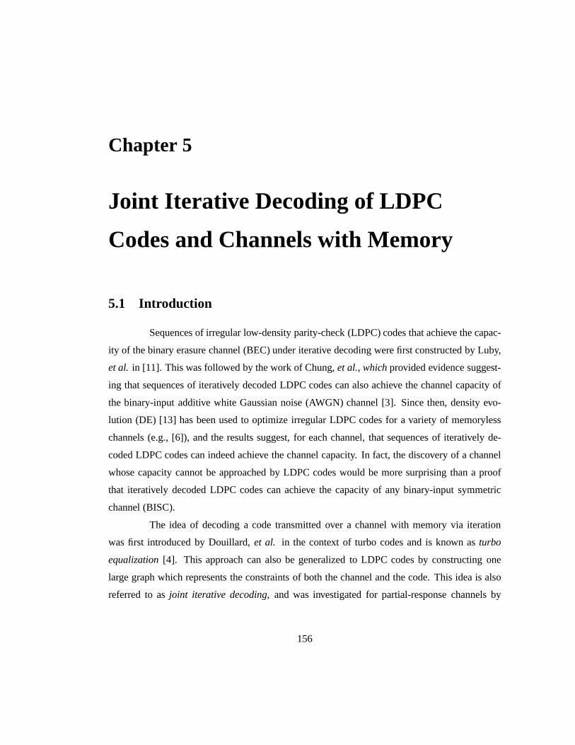
Figure 5.1.1: Block diagram of the system.
Kurkoski, Siegel, and Wolf in [9].
Until recently, it was difficult to compare the performance of turbo equalization with
channel capacity because the binary-input capacity of the channel was unknown. Recently, a
new method has gained acceptance for estimating the achievable information rates of finite state
channels (FSCs) [1][12]1, and a number of authors have begun designing LDPC based coding
schemes which approach the achievable information rates of these channels [8][12][21]. As is
the case with DE for general BISCs, the evaluation of code thresholds and the optimization of
these thresholds is done numerically. For FSCs, the analysis of this system is quite complex
because the BCJR algorithm [2] is used to decode the channel.
Since the capacity of a channel with memory is generally not achievable via equiprob-
able signaling, one can instead aim for the symmetric information rate (SIR) of the channel. The
SIR is defined as the maximum information rate achievable via random coding with equiproba-
ble input symbols. Since linear codes use all inputs equiprobably, the SIR is also the maximum
rate directly achievable with linear codes. In this chapter, we introduce a class of channels with
memory, which we refer to as generalized erasure channels (GECs). For these channels, we show
that DE can be done analytically for the joint iterative decoding of irregular LDPC codes and the
channel. This allows us to construct sequences of LDPC degree distributions which appear to
achieve the SIR using iterative decoding. As an example, we focus on the dicode erasure channel
(DEC), which is simply a binary-input channel with a linear response of1−D and erasure noise.
In Section 5.2, we introduce the basic components of our system. This includes the
joint iterative decoder, GECs and the DEC, and irregular LDPC codes. In Section 5.3, we derive
a single parameter recursion for the DE of the joint iterative decoder which allows us to give
necessary and sufficient conditions for decoder convergence. These conditions are also used to
construct code sequences which appear to achieve the SIR. In Section 5.4, we discuss extensions1This method was also introduced by Sharma and Singh in [14]. However, it appears that most of the other results
in their paper, based on regenerative theory, are actually incorrect. A correct analytical treatment can be found inSection 4.4.4.
158
Y 1 Y n
interleaver
channel detector
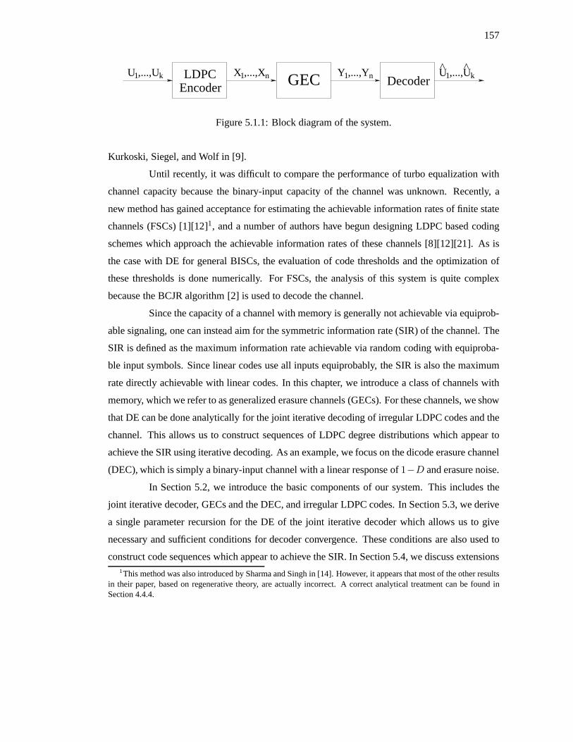
Figure 5.2.1: Gallager-Tanner-Wiberg graph of the joint iterative decoder.
to arbitrary GECs and describe a practical optimization technique based on linear programming.
Finally, we offer some concluding remarks in Section 5.5.
5.2 System Model
5.2.1 Description
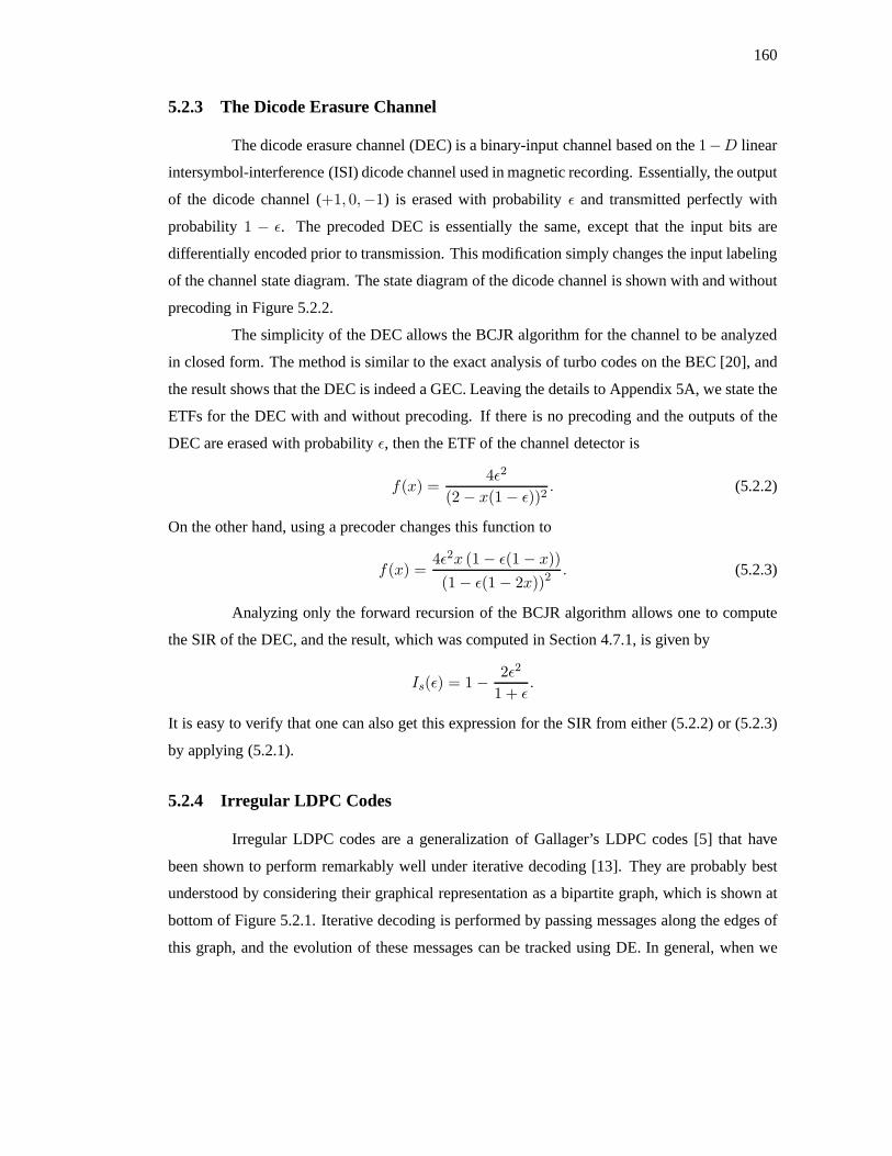
The system we consider is fairly standard for the joint iterative decoding of an LDPC
code and a channel with memory. Equiprobable information bits,U = U1, . . . , Uk, are encoded
into an LDPC codeword,X = X1, . . . ,Xn, which is observed through a GEC as the output
vector,Y = Y1, . . . , Yn. The decoder consists of ana posteriori probability(APP) detector
matched to the channel and an LDPC decoder. The first half of decoding iterationi entails
running the channel detector onY using thea priori information from the LDPC code. The
second half of decoding iterationi corresponds to executing one LDPC iteration using internal
edge messages from the previous iteration and the channel detector output. Figure 5.1.1 shows
the block diagram of the system, and Figure 5.2.1 shows the Gallager-Tanner-Wiberg (GTW)
graph of the joint iterative decoder.
5.2.2 The Generalized Erasure Channel
Since the messages passed around the GTW graph of the joint decoder are all log-
likelihood ratios (LLRs), DE involves tracking the evolution of the distribution of LLR messages
159
passed around the decoder. LetL be a random variable representing a randomly chosen LLR at
the output of the channel decoder. If the distribution ofL is supported on the set{−∞, 0,∞}andPr(L = −∞) = Pr(L = ∞), then we refer to it as asymmetric erasure distribution.
Such distributions are one dimensional, and are completely defined by the erasure probability
Pr(L = 0). Our closed form analysis of this system requires that all the densities involved in
DE are symmetric erasure distributions.
Definition 5.2.1. A generalized erasure channel(GEC) is any channel which satisfies the fol-
lowing condition for i.i.d. equiprobable inputs. The LLR distribution at the output of the channel
detector is a symmetric erasure distribution whenever thea priori LLR distribution is a symmet-
ric erasure distribution.
This allows DE of the joint iterative decoder to be represented by a single parameter
recursion. Letf(x) be a function which maps the erasure probability of thea priori LLR dis-
tribution, x, to the erasure probability at the output of the detector. The effect of the channel
on the DE depends only onf(x), which we refer to as theerasure transfer function(ETF) of
the GEC. This function is very similar to the mutual information transfer function,T (I), used
by the EXIT chart analysis of ten Brink [18]. Since the mutual information of a BEC with era-
sure probabilityx is 1 − x, the mutual information transfer function andf(x) are linked by the
identity,T (I) = 1 − f(1 − I).
A remarkable connection between the SIR of a channel,Is, and its mutual information
transfer function was also introduced by ten Brink in [19]. This result requires thatT (I) is
computed using a symmetric erasure distribution as thea priori LLR distribution. A clever
application of the chain rule for mutual information shows that
limn→∞
1nI(X1, . . . ,Xn;Y1, . . . , Yn) =
∫ 1
0T (I)dI.
Assuming the input process is i.i.d. and equiprobable makes the LHS equal the SIR, and using
T (I) = 1 − f(1 − I) allows us to simplify this expression to
Is =∫ 1
0T (I)dI = 1 −
∫ 1
0f(x)dx. (5.2.1)
Previously, we saw thatf(x) completely characterizes the DE properties of a GEC, and now we
see that it can also be used to compute the SIR.
160
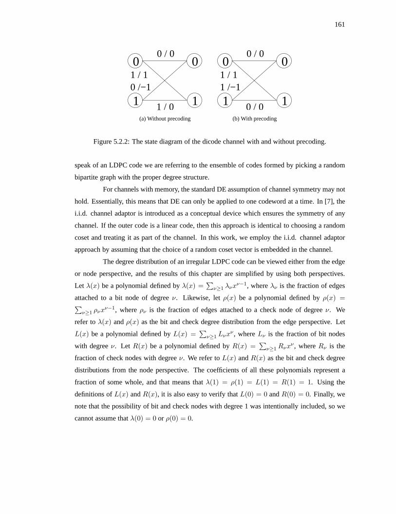
5.2.3 The Dicode Erasure Channel
The dicode erasure channel (DEC) is a binary-input channel based on the1−D linear
intersymbol-interference (ISI) dicode channel used in magnetic recording. Essentially, the output
of the dicode channel (+1, 0,−1) is erased with probabilityε and transmitted perfectly with
probability 1 − ε. The precoded DEC is essentially the same, except that the input bits are
differentially encoded prior to transmission. This modification simply changes the input labeling
of the channel state diagram. The state diagram of the dicode channel is shown with and without
precoding in Figure 5.2.2.
The simplicity of the DEC allows the BCJR algorithm for the channel to be analyzed
in closed form. The method is similar to the exact analysis of turbo codes on the BEC [20], and
the result shows that the DEC is indeed a GEC. Leaving the details to Appendix 5A, we state the
ETFs for the DEC with and without precoding. If there is no precoding and the outputs of the
DEC are erased with probabilityε, then the ETF of the channel detector is
f(x) =4ε2
(2 − x(1 − ε))2. (5.2.2)
On the other hand, using a precoder changes this function to
f(x) =4ε2x (1 − ε(1 − x))(1 − ε(1 − 2x))2
. (5.2.3)
Analyzing only the forward recursion of the BCJR algorithm allows one to compute
the SIR of the DEC, and the result, which was computed in Section 4.7.1, is given by
Is(ε) = 1 − 2ε2
1 + ε.
It is easy to verify that one can also get this expression for the SIR from either (5.2.2) or (5.2.3)
by applying (5.2.1).
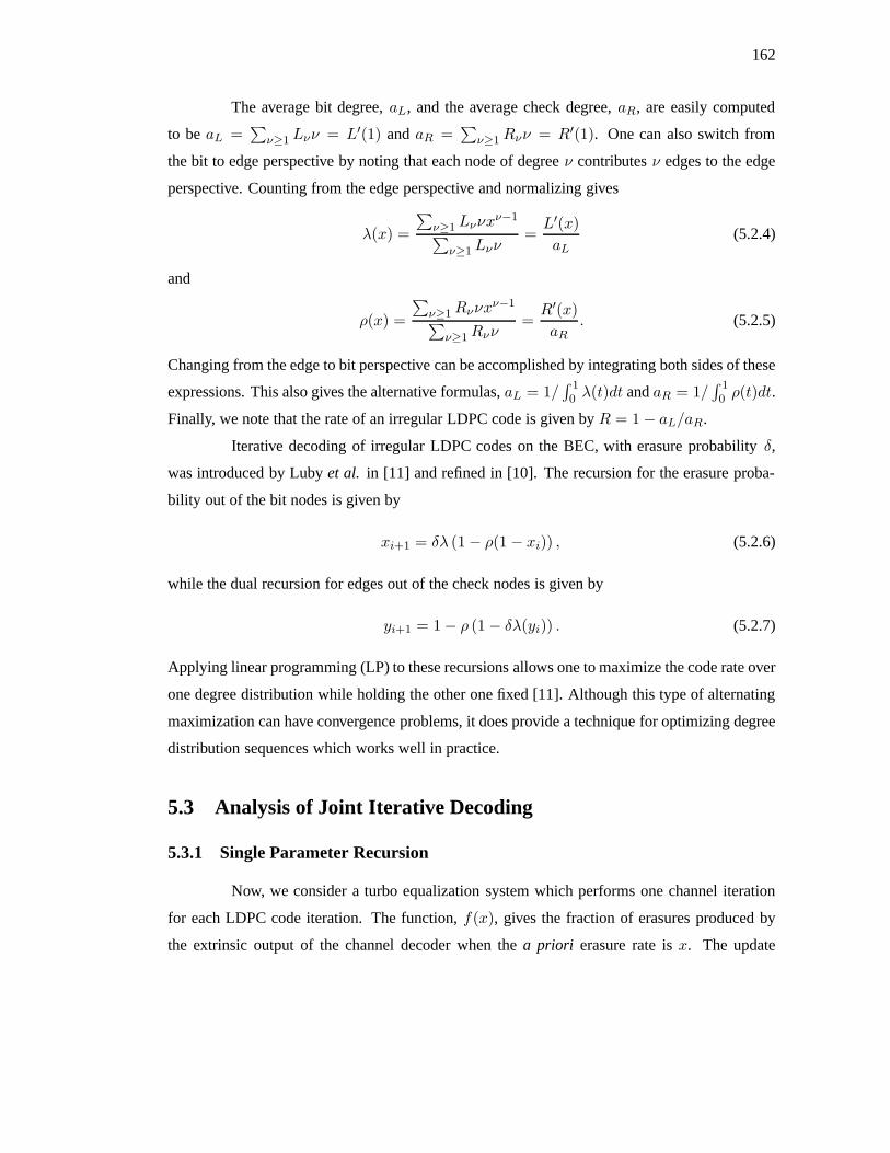
5.2.4 Irregular LDPC Codes
Irregular LDPC codes are a generalization of Gallager’s LDPC codes [5] that have
been shown to perform remarkably well under iterative decoding [13]. They are probably best
understood by considering their graphical representation as a bipartite graph, which is shown at
bottom of Figure 5.2.1. Iterative decoding is performed by passing messages along the edges of
this graph, and the evolution of these messages can be tracked using DE. In general, when we
161
0
11
0
0 /−11 / 1
1 / 0
0 / 0
(a) Without precoding
0
11
0
1 /−11 / 1
0 / 0
0 / 0
(b) With precoding
Figure 5.2.2: The state diagram of the dicode channel with and without precoding.
speak of an LDPC code we are referring to the ensemble of codes formed by picking a random
bipartite graph with the proper degree structure.
For channels with memory, the standard DE assumption of channel symmetry may not
hold. Essentially, this means that DE can only be applied to one codeword at a time. In [7], the
i.i.d. channel adaptor is introduced as a conceptual device which ensures the symmetry of any
channel. If the outer code is a linear code, then this approach is identical to choosing a random
coset and treating it as part of the channel. In this work, we employ the i.i.d. channel adaptor
approach by assuming that the choice of a random coset vector is embedded in the channel.
The degree distribution of an irregular LDPC code can be viewed either from the edge
or node perspective, and the results of this chapter are simplified by using both perspectives.
Let λ(x) be a polynomial defined byλ(x) =∑
ν≥1 λνxν−1, whereλν is the fraction of edges
attached to a bit node of degreeν. Likewise, letρ(x) be a polynomial defined byρ(x) =∑ν≥1 ρνx
ν−1, whereρν is the fraction of edges attached to a check node of degreeν. We
refer toλ(x) andρ(x) as the bit and check degree distribution from the edge perspective. Let
L(x) be a polynomial defined byL(x) =∑
ν≥1 Lνxν , whereLν is the fraction of bit nodes
with degreeν. Let R(x) be a polynomial defined byR(x) =∑
ν≥1Rνxν , whereRν is the
fraction of check nodes with degreeν. We refer toL(x) andR(x) as the bit and check degree
distributions from the node perspective. The coefficients of all these polynomials represent a
fraction of some whole, and that means thatλ(1) = ρ(1) = L(1) = R(1) = 1. Using the
definitions ofL(x) andR(x), it is also easy to verify thatL(0) = 0 andR(0) = 0. Finally, we
note that the possibility of bit and check nodes with degree 1 was intentionally included, so we
cannot assume thatλ(0) = 0 or ρ(0) = 0.
162
The average bit degree,aL, and the average check degree,aR, are easily computed
to beaL =∑
ν≥1 Lνν = L′(1) andaR =∑
ν≥1Rνν = R′(1). One can also switch from
the bit to edge perspective by noting that each node of degreeν contributesν edges to the edge
perspective. Counting from the edge perspective and normalizing gives
λ(x) =
∑ν≥1 Lννx
ν−1∑ν≥1 Lνν
=L′(x)aL
(5.2.4)
and
ρ(x) =
∑ν≥1Rννx
ν−1∑ν≥1Rνν
=R′(x)aR
. (5.2.5)
Changing from the edge to bit perspective can be accomplished by integrating both sides of these
expressions. This also gives the alternative formulas,aL = 1/∫ 10 λ(t)dt andaR = 1/
∫ 10 ρ(t)dt.
Finally, we note that the rate of an irregular LDPC code is given byR = 1 − aL/aR.
Iterative decoding of irregular LDPC codes on the BEC, with erasure probabilityδ,
was introduced by Lubyet al. in [11] and refined in [10]. The recursion for the erasure proba-
bility out of the bit nodes is given by
xi+1 = δλ (1 − ρ(1 − xi)) , (5.2.6)
while the dual recursion for edges out of the check nodes is given by
yi+1 = 1 − ρ (1 − δλ(yi)) . (5.2.7)
Applying linear programming (LP) to these recursions allows one to maximize the code rate over
one degree distribution while holding the other one fixed [11]. Although this type of alternating
maximization can have convergence problems, it does provide a technique for optimizing degree
distribution sequences which works well in practice.
5.3 Analysis of Joint Iterative Decoding
5.3.1 Single Parameter Recursion
Now, we consider a turbo equalization system which performs one channel iteration
for each LDPC code iteration. The function,f(x), gives the fraction of erasures produced by
the extrinsic output of the channel decoder when thea priori erasure rate isx. The update
163
equations for this system are almost identical to (5.2.6) and (5.2.7). The main difference is that
the parameterδ now changes with iteration and is written asδi.
Consider the messages passed from the output of the check nodes to the input of the
bit nodes, and letx be the fraction which are erased. Since any non-erasure message passed into
a bit node gives perfect knowledge of the bit, the messages at the output of the bit node will
only be erased only if all of the messages at the input to the bit node are erased. Therefore, the
fraction of erased messages passed back from a bit node of degreeν to the check nodes is given
by δixν−1. Using this, it is easy to verify that the fraction of erased messages passed back from
all the bit nodes to the check nodes is given byδi∑
ν≥1 λνxν−1 = δiλ(x).
There is also a fundamental difference between the messages passed from the bit nodes
to the check nodes and the messages passed from the bit nodes to the channel detector. This
difference is due to the fact that a degreeν bit node sendsν messages to the check nodes and
only 1 message to the channel detector. The fraction of erased messages passed from a degree
ν bit node to the channel detector is given byxν . Combining these two observations, shows
that the fraction of erased messages passed from all of the bit nodes to the channel detector is∑ν≥1 Lνx
ν = L(x).
The recursion for the erasure probability out of the bit nodes is now given by
xi+1 = δiλ (1 − ρ(1 − xi)) , (5.3.1)
whereδi = f (L (1 − ρ(1 − xi))) andx0 = f(1). Likewise, the dual recursion for edges out of
the check nodes is now given by
yi+1 = 1 − ρ (1 − δiλ(yi)) ,
whereδi = f (L(yi)) andy0 = 1 − ρ (1 − f(1)).
5.3.2 Conditions for Convergence
Using the recursion (5.3.1), we can derive a necessary and sufficient condition for the
erasure probability to converge to zero. This condition is typically written as a basic condition
which must hold forx ∈ (0, 1] and an auxiliary stability condition which simplifies the analysis
atx = 0. The basic condition implies there are no fixed points in the iteration forx ∈ (0, 1] and
is given by
f (L (1 − ρ(1 − x)))λ (1 − ρ(1 − x)) < x. (5.3.2)
164
Verifying this condition numerically for very smallx can be difficult, so we require instead that
x = 0 is a stable fixed point of the recursion. This is equivalent to evaluating the derivative of
(5.3.2) atx = 0, which gives the stability condition(λ2(0)f ′(0)aL + λ′(0)f(0)
)ρ′(1) < 1. (5.3.3)
The following facts make it easy to derive (5.3.3) from (5.3.2):ρ(1) = 1, L(0) = 0, and
L′(x) = aLλ(x).
Now, we can use (5.3.2) and (5.3.3) to say something about the code properties re-
quired by various channels.
1. If the channel hasf(0) > 0 and the code hasλ(0) > 0, thenf(0)λ(0) > 0 and (5.3.2)
cannot hold near zero. This means thatλ(0) = 0 is required for the satisfaction of (5.3.2),
and this implies that the code cannot have degree 1 bit nodes (i.e., bits with very little code
protection). In this case, the stability condition simplifies toλ2f(0)ρ′(1) ≤ 1.
2. If the channel hasf(0) = 0, then degree 1 bit nodes do not cause this problem. In this
case, the stability condition simplifies toλ21f
′(0)aLρ′(1) < 1.
3. If the channel hasf(1) = 1 and the code hasρ(0) = 0, then iteration cannot proceed
beyond the fixed point atx = 1. It follows that the code must haveρ(0) > 0 to get the
iteration started. In this case, the required degree 1 check nodes essentially act very much
like pilot bits.
The next step is mapping (5.3.2) into an equivalent condition which is easier to manipulate.
Consider the condition
f (L (1 − ρ(1 − q(x))))λ (1 − ρ(1 − q(x))) < q(x),
for any q(x) which is a one-to-one mapping from the interval(0, 1] to the interval(0, 1]. This
new condition is equivalent to the original condition (5.3.2). Choosingq(x) = 1 − ρ−1(1 − x)
collapses the basic condition to
f (L(x))λ(x) < q(x) (5.3.4)
becauseq−1(x) = 1 − ρ(1 − x). Using (5.2.4), we can substitute forλ(x) to get
f (L(x))L′(x) < aLq(x). (5.3.5)
165
Integrating both sides of this inequality from0 to x gives
F (L(x)) < aLQ(x),
whereF (x) =∫ x0 f(t)dt andQ(x) =
∫ x0 q(t)dt. We note that the functionF (x) is non-
decreasing forx ≥ 0 because the functionf(x) is non-negative forx ≥ 0. This means that
F (x) is invertible forx ≥ 0 and we can solve forL(x) by writing
L(x) < F−1 (aLQ(x)) . (5.3.6)
It appears that we now have a closed form condition involving onlyL(x) which can be used
to analyze the system. Unfortunately, this condition (5.3.6) does not imply (5.3.2) because the
sequence of transformations is not reversible. Integrating both sides of an inequality preserves
the inequality, but working backwards requires that we take the derivative of both sides. This
does not, in general, preserve the inequality.
One way to work around this problem is to require that each step of the above deriva-
tion holds with equality. If we assume that (5.3.6) holds with equality, then we can takes its
derivative and solve forλ(x) to get
λ(x) =q(x)
f (F−1 (aLQ(x))). (5.3.7)
It is easy to verify this step using the facts thatddxF
−1(x) = 1/f(F−1(x)
),Q′(x) = q(x), and
L′(x) = aLλ(x). Finally, we note that (5.3.7) implies that the basic condition (5.3.2) holds with
equality as well.
The following theorem relates these inequalities to the gap between the SIR and the
code rate.
Theorem 5.3.1. Consider any LDPC code ensemble, defined by the degree distributionsλ(x)
andρ(x), which satisfies (5.3.2) for some GEC with ETFf(x). The gap,∆, between the rate of
the LDPC code and the SIR of the channel,Is, is given by
∆ = Is −R =∫ 1
0g(x)dx,
whereg(x) = aLq(x) − f (L(x))L′(x) is the non-negative gap between the LHS and the RHS
of (5.3.5).
166
Proof. Evaluating the integral gives∫ 1
0g(x)dx = aL [Q(1) −Q(0)] − [F (L(1)) − F (L(0))] ,
whereQ(0) = 0, F (L(0)) = F (0) = 0, andF (L(1)) = F (1) = 1− Is. We can computeQ(1)
using the geometric fact that∫ 1
0ρ(x)dx +
∫ 1
0ρ−1(x)dx = 1,
and this gives
Q(1) =∫ 1
0
(1 − ρ−1(1 − x)
)dx =
∫ 1
0
(1 − ρ−1(x)
)dx =
∫ 1
0ρ(x)dx =
1aR.
Putting these together with the fact thatR = 1 − aL/aR gives∫ 1
0g(x)dx =
aL
aR− (1 − Is) = Is −R.
5.3.3 Achieving the Symmetric Information Rate
Now, we consider sequences of irregular LDPC code ensembles which can be used to
communicate reliably at rates arbitrarily close to the SIR. The code sequence is defined by the se-
quence of degree distributions{ρ(k)(x), λ(k)(x)
}k≥0
and its associated rate sequence{Rk}k≥0
is given byRk = 1 − a(k)L /a
(k)R via the results of Section 5.2.4. The main difficulty that we
will encounter while using algebraic methods to define code sequences is that the implied degree
distributions may not be non-negative and generally have infinite support. We say that a degree
distribution is (i)admissibleif its power series expansion aboutx = 0 has only non-negative
coefficients and (ii)realizable if it is a polynomial (i.e., finite degree) whose coefficients sum
to one. We say that a sequence of degree distributions isSIR achievingif, for any ε > 0, there
exists ank0 such that, for allk > k0, thekth degree distribution is (i) realizable, (ii) satisfies
(5.3.2), and (iii) has rateRk > Is − ε.
The following corollary of Theorem 5.3.1 provides a necessary and sufficient condition
for an SIR achieving sequence of degree distributions.
Corollary 5.3.2. Consider any sequence of LDPC code ensembles, defined by the sequence{ρ(k)(x), λ(k)(x)
}k≥0
of realizable degree distributions, which satisfy (5.3.2) for some GEC
167
with ETFf(x). This sequence of codes is SIR achieving if and only if the associated sequence
of rate gap functions, defined by
g(k)(x) = a(k)L
[q(k)(x) − f
(L(k)(x)
)λ(k)(x)
],
converges to zero almost everywhere on[0, 1].
Proof. The definition of SIR achieving requires that the associated sequence of rate gaps, defined
by ∆k =∫ 10 g
(k)(x)dx, approaches zero. Sinceg(k)(x) > 0 on (0, 1] by assumption, this
requires thatlimk→∞ g(k)(x) = 0 almost everywhere on[0, 1].
Remark 5.3.3.For the BEC, Shokrollahi [16] showed that all sequences of capacity achieving
codes obey a flatness condition which says that the sequence of non-negative gap functions
implied by the basic condition, defined by
f(L(k)
(1 − ρ(k)(1 − x)
))λ(k)
(1 − ρ(k)(1 − x)
)− x,
converges (along with all of its derivatives) to zero uniformly on[0, 1]. We believe this can
probably be extended to GECs under the assumption that the power series expansion off(x)
aboutx = 0 converges uniformly on[0, 1].
In general, we construct SIR achieving sequences by starting with a sequence of realizable check
degree distributions{ρ(k)(x)
}k≥0
and then using a slight variation of (5.3.7) to define a sequence
of bit degree distributions{λ(k)(x)
}k≥0
. If each bit degree distribution in this sequence is
admissible withλ(k)(1) > 1, then we can form the sequence of realizable bit degree distributions{λ(k)(x)
}k≥0
by truncating the power series of eachλ(k)(x) so thatλ(k)(1) = 1. Specifically,
we generalize the notation of Section 5.2.4 and letλ(k)i = λ
(k)i for 1 ≤ i < Nk, whereNk is the
smallest integer such that∑Nk
i=1 λ(k)i ≥ 1. The last termλ(k)
Nkis then chosen so thatλ(k)(1) = 1.
One problem with this method, which does not occur for the BEC [15], is that the
truncation may cause the basic condition (5.3.2) to fail. To overcome this problem, we require
the codes in sequence to satisfy the slightly stronger condition that
(1 + αk)f(L(k)(x)
)λ(k)(x) = q(k)(x), (5.3.8)
where L(k)(x) =∫ x0 λ
(k)(t)dt/∫ 10 λ
(k)(t)dt and q(k)(x) = 1 −(ρ(k)
)−1(1 − x). This is
essentially the same as designing codes for a sequence of degraded channels given byf (k)(x) =
168
(1 + αk)f(x). Adapting (5.3.6) to our system with equality gives
L(k)(x) = F−1
(1
1 + αka
(k)L Q(k)(x)
), (5.3.9)
whereQ(k)(x) =∫ x0 q
(k)(t)dt. Requiring thatL(k)(1) = 1 is the same as choosinga(k)L so that,
without truncation, the code rate equals the SIR of the degraded channel. This gives
a(k)L = a
(k)R (1 + αk)F (1), (5.3.10)
because from (5.2.1) we haveIs = 1 − F (1). Taking the derivative of (5.3.9) and substituting
for a(k)L with (5.3.10) gives
λ(k)(x) =q(k)(x)
(1 + αk)f(F−1
(F (1)a(k)
R Q(k)(x))) . (5.3.11)
Notice that the channel only enters this equation via the expressionf(F−1 (F (1)x)
)and that
varyingαk really only changes the truncation point forλ(k)(x). Using the facts thatq(k)(x) = 1
andQ(k)(1) = 1/a(k)R , we also note that
λ(k)(1) =1
(1 + αk)f(1). (5.3.12)
This means that the truncation will work, for small enoughαk, as long asf(1) < 1.
Theorem 5.3.4. Let{ρ(k)(x)
}k≥0
be a sequence of realizable check degree distributions and
let{λ(k)(x)
}k≥0
be the sequence of bit degree distributions given by (5.3.11). Suppose that (i)
the first derivative off(x) is bounded on[0, 1] andf(1) < 1, (ii) eachλ(k)(x) given by (5.3.11)
with αk = 0 is admissible, and (iii) the average check degreea(k)R and maximum bit degreeNk
satisfya(k)R /Nk → 0. Under these conditions, there exists a positive sequence{αk}k≥0 such
that the sequence of degree distributions{ρ(k)(x), λ(k)(x)
}k≥0
defined above is SIR achieving.
Proof. We start by examining the effect of the power series truncation. This gives the the sand-
wich inequality
λ(k)(x) −(λ(k)(1) − 1
)xNk−1 ≤ λ(k)(x) < λ(k)(x), (5.3.13)
where the LHS holds because(λ(k)(1) − 1
)xNk−1 is an upper bound on the truncated terms
and the RHS holds by truncation of positive terms. Now, consider the integral representation,
169
L(k)(x) =∫ x0 λ
(k)(t)dt/∫ 10 λ
(k)(t)dt, implied by integrating (5.2.4). Using this and (5.3.13),
we get a sandwich inequality forL(k)(x) given by∫ x0
(λ(k)(t) −
(λ(k)(1) − 1
)tNk−1
)dt∫ 1
0 λ(k)(t)dt
< L(k)(x) <
∫ x0 λ
(k)(t)dt∫ 10
(λ(k)(t) −
(λ(k)(1) − 1
)tNk−1
)dt,
whereλ(k)(x) is upper/lower bounded by the RHS/LHS of (5.3.13) respectively. Evaluating the
integrals and rearranging terms reduces this to
L(k)(x) − βkxNk < L(k)(x) <
11 − βk
L(k)(x), (5.3.14)
whereβk =(λ(k)(1) − 1
)a
(k)L /Nk. Using (5.3.10) and (5.3.12), we also see that
βk =(
1(1 + αk)f(1)
− 1)a
(k)R (1 + αk)(1 − Is)
Nk≤ a
(k)R (1 − Is)f(1)Nk
= O
(a
(k)R
Nk
). (5.3.15)
Now, we use these results to analyze the convergence condition for the true channel.
First, we defineαk to take the smallest value such that
f(L(k)(x)
)λ(k)(x) < q(k)(x) (5.3.16)
for all x ∈ (0, 1], whereL(k)(x) andλ(k)(x) depend implicitly onαk through the truncation of
(5.3.11). Using this value forαk means that, by definition,{ρ(k)(x), λ(k)(x)
}k≥0
is a sequence
of realization degree distributions which satisfies the basic condition. Next, we derive an upper
bound on the value ofαk chosen. Using (5.3.13) and (5.3.14), it is easy to verify that the
condition,
f
(1
1 − βkL(k)(x)
)λ(k)(x) ≤ q(k)(x), (5.3.17)
is more stringent than (5.3.16) and therefore implies (5.3.16). Using (5.3.8) to substitute for
q(k)(x), we can then solve for the smallestαk that implies (5.3.17). The result is the upper
bound,
αk ≤ max0≤x≤1
f
(1
1 − βkL(k)(x)
)/f(L(k)(x)
)− 1, (5.3.18)
because anyαk which satisfies this condition must imply (5.3.17) and (5.3.16).
170
Finally, we show that the sequence of rate gaps∆k = Is − Rk converges to zero.
Using the LHS of (5.3.13) and the integral form ofa(k)L , we can write
1
a(k)L
≥∫ 1
0
(λ(k)(x) −
(λ(k)(1) − 1
)xNk−1
)dx =
1
a(k)L
− λ(k)(1) − 1Nk
= (1 − βk)1
a(k)L
.
Using this and (5.3.10), we can lower bound the code rate with
Rk ≥ 1 − a(k)L
a(k)R (1 − βk)
= 1 − (1 + αk)(1 − Is)1 − βk
.
This means that the rate gap is upper bounded by
∆k ≤ Is(1 − βk)1 − βk
− (1 − βk) − (1 + αk)(1 − Is)1 − βk
=(αk + βk)(1 − Is)
1 − βk.
Combining the assumption thata(k)R /Nk → 0 with (5.3.15) shows thatβk → 0. Since the first
derivative off(x) is bounded, we can also combineβk → 0 with (5.3.18) to show thatαk → 0.
In fact, examining (5.3.18) more closely shows thatαk = O (βk) which means the rate gap is
also∆k = O (βk) = O(a
(k)R /Nk
). This completes the proof.
5.3.4 Degree Sequences with Regular Check Distributions
In this section, we limit our scope somewhat by choosing check distributions with a
single non-zero coefficient. This type of check distribution is called regular, and is defined by
ρ(k)(x) = xk−1. This implies thatq(k)(x) = 1 − (1 − x)1/(k−1) andQ(k)(x) = (k − 1)(1 −x)k/(k−1)/k + x, and we use these to rewrite (5.3.11) as
λ(k)(x) =1 − (1 − x)1/(k−1)
(1 + αk)f(F−1
(F (1) (k−1)(1−x)k/(k−1)+kx
k
)) .As shown in [15], the non-negative power series expansion of1 − (1 − x)1/(k−1) is given by
1 − (1 − x)1/(k−1) =∞∑i=1
(1/(k − 1)
i
)(−1)i+1xi.
This means that question of whether or notλ(k)(x) has a non-negative power series expansion is
very much linked to the power series expansion ofh(x) , 1/f(F−1 (F (1)x)
). While answer-
ing this question is difficult, we can still make general comments. For one, this method appears
to be doomed if the coefficients ofh(x) do not decay to zero. Since the location of the smallest
171
0 5 10 15 200
0.2
0.4
λ(4)
0 5 10 15 200
0.2λ(5)
0 5 10 15 200
0.1
0.2
λ(6)
0 5 10 15 200
0.1
0.2
λ(7)
degree
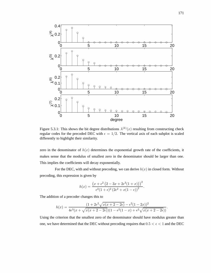
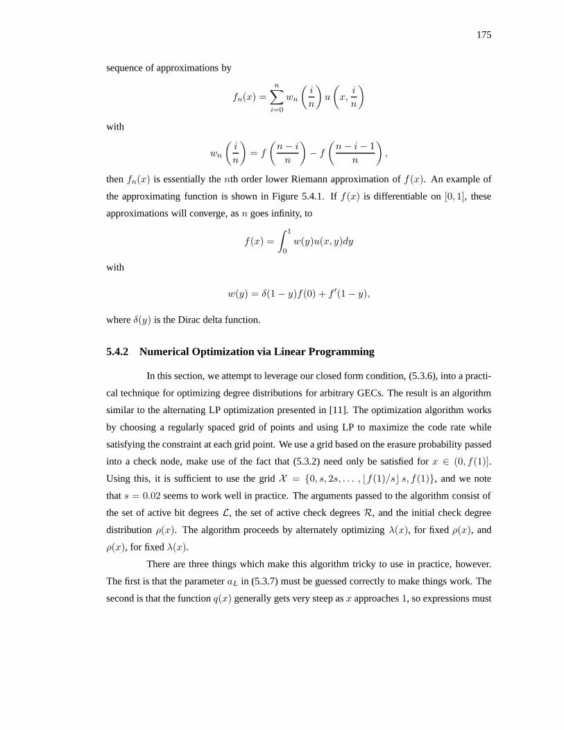
Figure 5.3.1: This shows the bit degree distributionsλ(k)(x) resulting from constructing checkregular codes for the precoded DEC withε = 1/2. The vertical axis of each subplot is scaleddifferently to highlight their similarity.
zero in the denominator ofh(x) determines the exponential growth rate of the coefficients, it
makes sense that the modulus of smallest zero in the denominator should be larger than one.
This implies the coefficients will decay exponentially.
For the DEC, with and without precoding, we can deriveh(x) in closed form. Without
precoding, this expression is given by
h(x) =
(x+ ε2
(2 − 3x+ 2ε3(1 + x)
))2ε2(1 + ε)2 (2ε2 + x(1 − ε))2
.
The addition of a precoder changes this to
h(x) =(1 + 2ε2
√x(x+ 2 − 2ε) − ε2(1 − 2x))2
4ε3(x+√x(x+ 2 − 2ε))(1 − ε2(1 − x) + ε2
√x(x+ 2 − 2ε))
.
Using the criterion that the smallest zero of the denominator should have modulus greater than
one, we have determined that the DEC without precoding requires that0.5 < ε < 1 and the DEC
172
k a(k)R a
(k)L Rk ∆k Nk αk βk λ
(k)1 λ
(k)1
4 4 1.595 0.6011 0.0655 4 0.16 0.4844 0.3127 0.3048
5 5 1.903 0.6193 0.0473 7 0.069 0.3937 0.2563 0.2562
6 6 2.102 0.6496 0.0170 9 0.048 0.2671 0.2181 0.2134
7 7 2.411 0.6555 0.0111 19 0.025 0.1681 0.1991 0.1843
8 8 2.718 0.6602 0.0064 33 0.014 0.1063 0.1615 0.1614
9 9 3.030 0.6632 0.0034 56 0.0075 0.0666 0.1436 0.1433
10 10 3.349 0.6651 0.0016 101 0.0042 0.0411 0.1287 0.1286
11 11 3.677 0.6657 0.0009 184 0.0023 0.0249 0.1166 0.1165
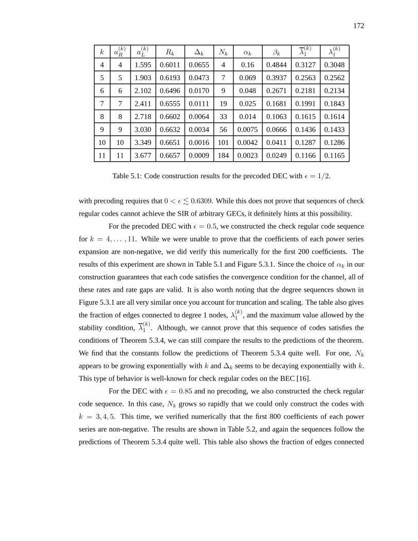
Table 5.1: Code construction results for the precoded DEC withε = 1/2.
with precoding requires that0 < ε . 0.6309. While this does not prove that sequences of check
regular codes cannot achieve the SIR of arbitrary GECs, it definitely hints at this possibility.
For the precoded DEC withε = 0.5, we constructed the check regular code sequence
for k = 4, . . . , 11. While we were unable to prove that the coefficients of each power series
expansion are non-negative, we did verify this numerically for the first 200 coefficients. The
results of this experiment are shown in Table 5.1 and Figure 5.3.1. Since the choice ofαk in our
construction guarantees that each code satisfies the convergence condition for the channel, all of
these rates and rate gaps are valid. It is also worth noting that the degree sequences shown in
Figure 5.3.1 are all very similar once you account for truncation and scaling. The table also gives
the fraction of edges connected to degree 1 nodes,λ(k)1 , and the maximum value allowed by the
stability condition,λ(k)1 . Although, we cannot prove that this sequence of codes satisfies the
conditions of Theorem 5.3.4, we can still compare the results to the predictions of the theorem.
We find that the constants follow the predictions of Theorem 5.3.4 quite well. For one,Nk
appears to be growing exponentially withk and∆k seems to be decaying exponentially withk.
This type of behavior is well-known for check regular codes on the BEC [16].
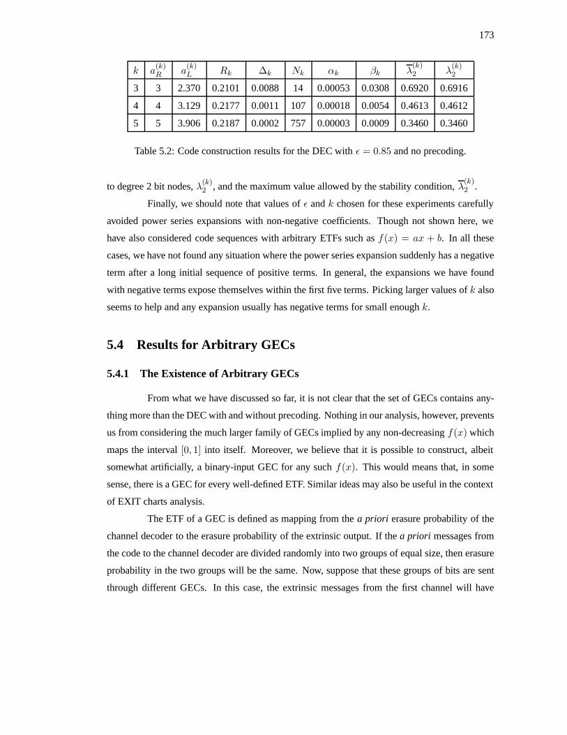
For the DEC withε = 0.85 and no precoding, we also constructed the check regular
code sequence. In this case,Nk grows so rapidly that we could only construct the codes with
k = 3, 4, 5. This time, we verified numerically that the first 800 coefficients of each power
series are non-negative. The results are shown in Table 5.2, and again the sequences follow the
predictions of Theorem 5.3.4 quite well. This table also shows the fraction of edges connected
173
k a(k)R a
(k)L Rk ∆k Nk αk βk λ
(k)2 λ
(k)2
3 3 2.370 0.2101 0.0088 14 0.00053 0.0308 0.6920 0.6916
4 4 3.129 0.2177 0.0011 107 0.00018 0.0054 0.4613 0.4612
5 5 3.906 0.2187 0.0002 757 0.00003 0.0009 0.3460 0.3460
Table 5.2: Code construction results for the DEC withε = 0.85 and no precoding.
to degree 2 bit nodes,λ(k)2 , and the maximum value allowed by the stability condition,λ
(k)2 .
Finally, we should note that values ofε andk chosen for these experiments carefully
avoided power series expansions with non-negative coefficients. Though not shown here, we
have also considered code sequences with arbitrary ETFs such asf(x) = ax + b. In all these
cases, we have not found any situation where the power series expansion suddenly has a negative
term after a long initial sequence of positive terms. In general, the expansions we have found
with negative terms expose themselves within the first five terms. Picking larger values ofk also
seems to help and any expansion usually has negative terms for small enoughk.
5.4 Results for Arbitrary GECs
5.4.1 The Existence of Arbitrary GECs
From what we have discussed so far, it is not clear that the set of GECs contains any-
thing more than the DEC with and without precoding. Nothing in our analysis, however, prevents
us from considering the much larger family of GECs implied by any non-decreasingf(x) which
maps the interval[0, 1] into itself. Moreover, we believe that it is possible to construct, albeit
somewhat artificially, a binary-input GEC for any suchf(x). This would means that, in some
sense, there is a GEC for every well-defined ETF. Similar ideas may also be useful in the context
of EXIT charts analysis.
The ETF of a GEC is defined as mapping from thea priori erasure probability of the
channel decoder to the erasure probability of the extrinsic output. If thea priori messages from
the code to the channel decoder are divided randomly into two groups of equal size, then erasure
probability in the two groups will be the same. Now, suppose that these groups of bits are sent
through different GECs. In this case, the extrinsic messages from the first channel will have
174
0 0.2 0.4 0.6 0.8 10.2
0.25
0.3
0.35
0.4
0.45
0.5
x
f 10(x
)
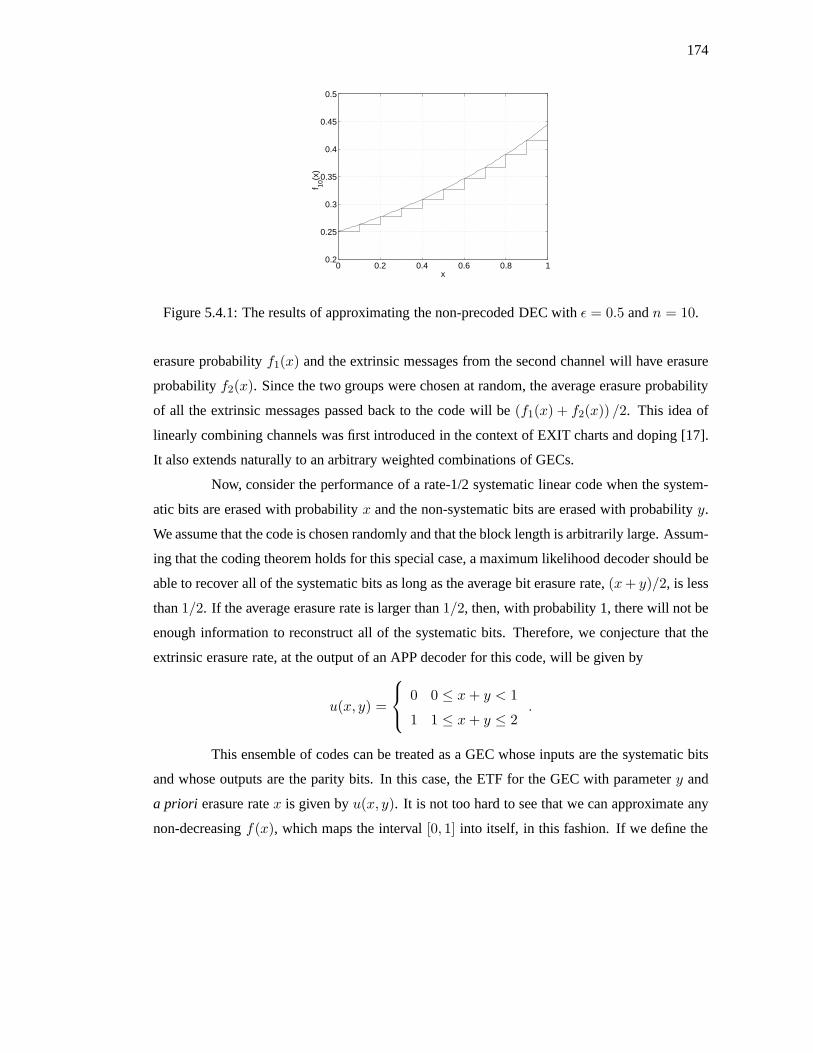
Figure 5.4.1: The results of approximating the non-precoded DEC withε = 0.5 andn = 10.
erasure probabilityf1(x) and the extrinsic messages from the second channel will have erasure
probabilityf2(x). Since the two groups were chosen at random, the average erasure probability
of all the extrinsic messages passed back to the code will be(f1(x) + f2(x)) /2. This idea of
linearly combining channels was first introduced in the context of EXIT charts and doping [17].
It also extends naturally to an arbitrary weighted combinations of GECs.
Now, consider the performance of a rate-1/2 systematic linear code when the system-
atic bits are erased with probabilityx and the non-systematic bits are erased with probabilityy.
We assume that the code is chosen randomly and that the block length is arbitrarily large. Assum-
ing that the coding theorem holds for this special case, a maximum likelihood decoder should be
able to recover all of the systematic bits as long as the average bit erasure rate,(x+ y)/2, is less
than1/2. If the average erasure rate is larger than1/2, then, with probability 1, there will not be
enough information to reconstruct all of the systematic bits. Therefore, we conjecture that the
extrinsic erasure rate, at the output of an APP decoder for this code, will be given by
u(x, y) =
0 0 ≤ x+ y < 1
1 1 ≤ x+ y ≤ 2.
This ensemble of codes can be treated as a GEC whose inputs are the systematic bits
and whose outputs are the parity bits. In this case, the ETF for the GEC with parametery and
a priori erasure ratex is given byu(x, y). It is not too hard to see that we can approximate any
non-decreasingf(x), which maps the interval[0, 1] into itself, in this fashion. If we define the
175
sequence of approximations by
fn(x) =n∑
i=0
wn
(i
n
)u
(x,i
n
)with
wn
(i
n
)= f
(n− i
n
)− f
(n− i− 1
n
),
thenfn(x) is essentially thenth order lower Riemann approximation off(x). An example of
the approximating function is shown in Figure 5.4.1. Iff(x) is differentiable on[0, 1], these
approximations will converge, asn goes infinity, to
f(x) =∫ 1
0w(y)u(x, y)dy
with
w(y) = δ(1 − y)f(0) + f ′(1 − y),
whereδ(y) is the Dirac delta function.
5.4.2 Numerical Optimization via Linear Programming
In this section, we attempt to leverage our closed form condition, (5.3.6), into a practi-
cal technique for optimizing degree distributions for arbitrary GECs. The result is an algorithm
similar to the alternating LP optimization presented in [11]. The optimization algorithm works
by choosing a regularly spaced grid of points and using LP to maximize the code rate while
satisfying the constraint at each grid point. We use a grid based on the erasure probability passed
into a check node, make use of the fact that (5.3.2) need only be satisfied forx ∈ (0, f(1)].
Using this, it is sufficient to use the gridX = {0, s, 2s, . . . , bf(1)/sc s, f(1)}, and we note
thats = 0.02 seems to work well in practice. The arguments passed to the algorithm consist of
the set of active bit degreesL, the set of active check degreesR, and the initial check degree
distribution ρ(x). The algorithm proceeds by alternately optimizingλ(x), for fixed ρ(x), and
ρ(x), for fixedλ(x).
There are three things which make this algorithm tricky to use in practice, however.
The first is that the parameteraL in (5.3.7) must be guessed correctly to make things work. The
second is that the functionq(x) generally gets very steep asx approaches1, so expressions must
176
be evaluated carefully to avoid numerical problems. The third is that LP is used to maximize the
rate under a constraint similar to (5.3.7), but we know this constraint does not imply that (5.3.2)
holds as well. The algorithm is stabilized by the fact that theρ(x) optimization always produces
a valid code which satisfies (5.3.2). Furthermore, if the algorithm converges, then (5.3.7) will
be satisfied with near equality which implies that (5.3.2) will also be satisfied with near equality.
All of these add up to an algorithm that can work quite well, albeit with some tweaking of the
initial conditions. Lastly, the convergence is rarely monotonic and the algorithm may initially
wander through terrible codes (i.e. negative rate) before finding a very good code.
Consider optimizingρ(x) for some fixedλ(x). The goal of maximizing the code rate
for fixedλ(x) is equivalent to minimizing the linear objective function,
1/aR =∑ν∈R
ρv1ν, (5.4.1)
because the code rate is1 − aL/aR. The LP constraints can be derived by starting with (5.3.4)
and applyingq−1(x) to both sides to get
q−1 (f (L(x)) λ(x)) < x.
Sinceq−1(x) = 1 − ρ(1 − x), this inequality can be rewritten as∑ν∈R
ρν
(1 − (1 − f (L(x))λ(x))ν−1
)< x,
which is linear in theρν ’s. In practice, we have found that the numerical robustness is improved
by lettingφ(x) equal theρ(x) from the previous iteration, and requiring that∑ν∈R
ρν
(1 − (1 − f (L (1 − φ(1 − x)))λ (1 − φ(1 − x)))ν−1
)< 1 − φ(1 − x) (5.4.2)
be satisfied for allx ∈ X . The stability condition, (5.3.3), can also be handled via the extra
inequality
∑ν∈R
ρν(ν − 1) <
1/(λ2
1f′(0)aL
)if f(0) = 0
1/ (λ2f(0)) if f(0) > 0.
Now, we consider optimizingλ(x) for fixed ρ(x). Our goal of maximizing the code
rate for fixedρ(x) is equivalent to maximizing the linear objective function,
1/aL =∑ν∈L
λv1ν, (5.4.3)
177
because the code rate is1 − aL/aR. The LP constraints can be derived by starting with (5.3.7),
substituting1 − ρ(1 − x) for x, and transforming it into an inequality to get
λ (1 − ρ(1 − x)) <x
f (F−1 (aLQ (1 − ρ(1 − x)))).
One subtlety is choosing theaL so the algorithm performs well. We have found that choosing
aL = F (1)/aR, which implicitly assumes that we will achieve the SIR, does the trick. Adding
the relaxation constant,c, and rewriting this gives the linear inequality,∑ν∈L
λν (1 − ρ(1 − x))ν−1 <cx
f (F−1 (F (1)aRQ (1 − ρ(1 − x)))), (5.4.4)
which must be satisfied for allx ∈ X . It is worth pointing out the similarity between (5.4.4) and
(5.3.11) withc playing the role ofαk. The stability condition, (5.3.3), depends on the channel
and is given by
λ1 < c√
1f ′(0)aLρ′(1) if f(0) = 0
λ2 <c
f(0)ρ′(1) if f(0) > 0
The relaxation constant is used to improve convergence and we typically usec = 1− (0.1)1+i/4
for theith λ(x) optimization.
In our implementation, all of the function evaluations required are done via linear in-
terpolation from sampled function tables. For example, we start by samplingf(x) on a very fine
grid. Next, we letF (x) be the integral of linear interpolatedf(x), which is given by trapezoidal
integration of thef(x) sample table. Inverse functions can also be handled by via linear inter-
polation. To do this, one simply reverses the role of the sampling grid and the sampled function
table. Finally, the functionQ (1 − ρ(1 − x)) can be computed accurately and efficiently using
Q (1 − ρ(1 − x)) =∑ν∈R
ρν
(1 − (1 − x)ν
ν− x(1 − x)ν−1
). (5.4.5)
Remark 5.4.1.This formula forQ (1 − ρ(1 − x)) can be derived by noticing that the rectangle
extending from(0, 0) to (x, q(x)) can be divided into two regions by the curveq(t) with t ∈[0, x]. Using the fact that the area of these two regions must sum toxq(x), we have∫ x
0q(t)dt+
∫ q(x)
0q−1(t)dt = xq(x).
178
This allows us to compute the integral ofq(x) with
Q(x) =∫ x
0q(t)dt
= xq(x) −∫ q(x)
0q−1(t)dt
= xq(x) −∫ q(x)
0(1 − ρ(1 − t)) dt
= xq(x) −∑ν≥1
ρν
(q(x) − 1 − (1 − q(x))ν
ν
).
Finally, we evaluate this expression by substituting1 − ρ(1 − y) = q−1(y) for x to get
Q (1 − ρ(1 − y)) = (1 − ρ(1 − y)) y −∑ν≥1
ρν
(y − 1 − (1 − y)ν
ν
).
Expandingρ(1 − y) and simplifying gives (5.4.5).
5.4.3 A Stability Condition for General Channels
In this section, we discuss one implication that this research has on the joint itera-
tive decoding of LDPC codes and general channels with memory. This implication is that the
stability condition for general channels may actually be as simple as the stability condition for
memoryless channel. Recall that, as long asf(0) > 0, the stability condition for GECs is given
by λ2ρ′(1)f(0) < 1. This condition is identical to the stability condition for the memoryless
erasure channel with erasure probabilityf(0). Let F0(x) be the LLR density at the extrinsic
output of the channel decoder, for a general channel, when perfecta priori information is passed
to the decoder. As long asF0(x) does not have perfect information itself (i.e., it is not equal
to a delta function at infinity), then the stability condition is given by applying the memoryless
channel condition from [13] toF0(x). This makes sense because, when the joint decoder is near
convergence, the LLRs passed asa priori information to the channel decoder are nearly error
free. A more rigorous analysis of this phenomenon is given in Appendix 5B.3.
5.5 Concluding Remarks
In this chapter, we consider the joint iterative decoding of irregular LDPC codes and
channels with memory. We introduce a new class of erasure channels with memory, known as
179
generalized erasure channels (GECs). For these channels, we derive a single parameter recur-
sion for density evolution of the joint iterative decoder. This allows us to state necessary and
sufficient conditions for decoder convergence and to algebraically construct sequences of LDPC
degree distributions which appear to approach the symmetric information rate of the channel.
This provides the first possibility of proving that the SIR is actually achievable via iterative de-
coding. In the future, we hope to prove that the two degree sequences constructed in this chapter
actually achieve the SIR. The bigger question is whether or not it is possible to construct degree
distribution sequences which achieve the SIR for any GEC.
5A Exact Analysis of the BCJR Decoder for the DEC
In this section, we analyze the behavior of a BCJR decoder for a DEC with erasure
rateε. This is achieved by first finding the steady state distributions of the forward and backward
recursions, and then computing the extrinsic erasure rate of the decoded input stream. Prior
knowledge of the input is taken into account by assuming that it is observed independently
through a BEC with erasure rateδ. This approach makes it possible to derive closed form
expressions for a system which combines a low density parity check (LDPC) code with a BCJR
decoder for this channel. Throughout this section, we assume that the channel inputs are chosen
i.i.d. B(1/2).
5A.1 The Dicode Erasure Channel without Precoding
Consider the BCJR algorithm operating on a DEC without precoding. In this section,
we compute the extrinsic erasure rate of that decoder as an explicit function of the channel
erasure rate,ε, and thea priori erasure rate,δ. This is done by analyzing the forward recursion,
the backward recursion, and the output stage separately.
Expanding our decoder to considera priori information is very similar to expanding
the alphabet of our channel. Instead of receiving a single output symbol from the setY =
{−, 0,+, e}, we receive a pair of output symbols. One is from the setY and the other, which
represents thea priori symbol, is from the setW = {0, 1, e} . Since the channel has only two
states, it suffices to consider the quantityα(t) , α(t)0 = 1 − α
(t)1 = Pr(St = 0|Wt−1
1 ,Yt−11 ).
The real simplification, however, comes from the fact that the distribution ofα(t) has finite
180
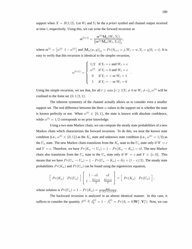
support whenX ∼ B(1/2). LetWt andYt be thea priori symbol and channel output received
at timet, respectively. Using this, we can write the forward recursion as
α(t+1) =α(t)Mα(Wt, Yt)∥∥α(t)Mα(Wt, Yt)
∥∥1
,
whereα(t) =[α(t) 1 − α(t)
]and[Mα(w, y)]ij = Pr(St+1 = j,Wt = w, Yt = y|St = i). It is
easy to verify that this recursion is identical to the simpler recursion,
α(t+1) =
1/2 if Yt = e andWt = e
α(t) if Yt = 0 andWt = e
0 if Yt = + orWt = 1
1 if Yt = − orWt = 0
.
Using the simple recursion, we see that, for allt ≥ min {i ≥ 1|Yi 6= 0 orWi 6= e}, α(t) will be
confined to the finite set{0, 1/2, 1}.
The inherent symmetry of the channel actually allows us to consider even a smaller
support set. The real difference between the threeα values in the support set is whether the state
is known perfectly or not. Whenα(t) ∈ {0, 1}, the state is known with absolute confidence,
while α(t) = 1/2 corresponds to no prior knowledge.
Using a two state Markov chain, we can compute the steady state probabilities of a new
Markov chain which characterizes the forward recursion. To do this, we treat the known state
condition (i.e.,α(t) ∈ {0, 1}) as theKα state and unknown state condition (i.e.,α(t) = 1/2) as
theUα state. The new Markov chain transitions from theKα state to theUα state only ifW = e
andY = e. Therefore, we havePr(Kα → Uα) = 1 − Pr(Kα → Kα) = εδ. The new Markov
chain also transitions from theUα state to theUα state only ifW = e andY ∈ {e, 0}. This
means that we havePr(Uα → Uα) = 1−Pr(Uα → Kα) = δ(ε+ (1− ε)/2). The steady state
probabilitiesPr(Kα) andPr(Uα) can be found using the eigenvector equation,
[Pr(Kα) Pr(Uα)
] 1 − εδ εδ
1 − δ(1+ε)2
δ(1+ε)2
=[Pr(Kα) Pr(Uα)
],
whose solution isPr(Uα) = 1 − Pr(Kα) = 2εδ2−δ(1+ε)+2εδ .
The backward recursion is analyzed in an almost identical manner. In this case, it
suffices to consider the quantityβ(t) , β(t)0 = 1 − β
(t)1 = Pr(St = 0|Wn
t ,Ynt ). Now, we can
181
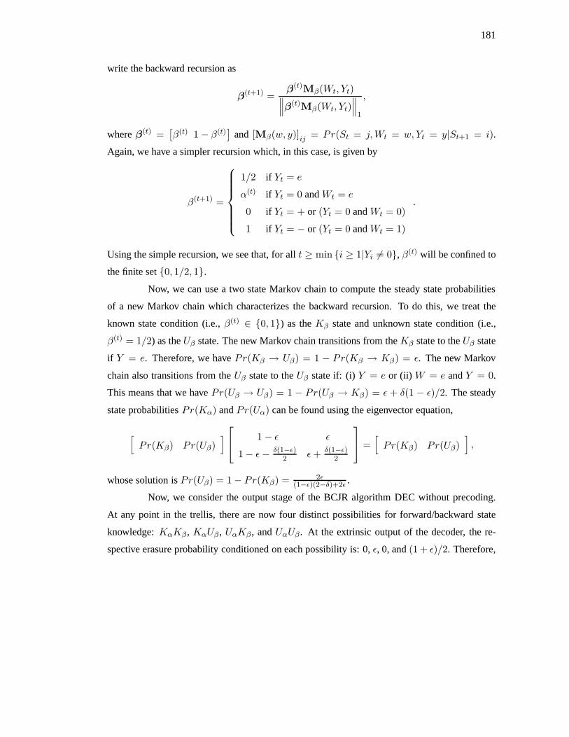
write the backward recursion as
β(t+1) =β(t)Mβ(Wt, Yt)∥∥∥β(t)Mβ(Wt, Yt)
∥∥∥1
,
whereβ(t) =[β(t) 1 − β(t)
]and [Mβ(w, y)]ij = Pr(St = j,Wt = w, Yt = y|St+1 = i).
Again, we have a simpler recursion which, in this case, is given by
β(t+1) =
1/2 if Yt = e
α(t) if Yt = 0 andWt = e
0 if Yt = + or (Yt = 0 andWt = 0)
1 if Yt = − or (Yt = 0 andWt = 1)
.
Using the simple recursion, we see that, for allt ≥ min {i ≥ 1|Yi 6= 0}, β(t) will be confined to
the finite set{0, 1/2, 1}.
Now, we can use a two state Markov chain to compute the steady state probabilities
of a new Markov chain which characterizes the backward recursion. To do this, we treat the
known state condition (i.e.,β(t) ∈ {0, 1}) as theKβ state and unknown state condition (i.e.,
β(t) = 1/2) as theUβ state. The new Markov chain transitions from theKβ state to theUβ state
if Y = e. Therefore, we havePr(Kβ → Uβ) = 1 − Pr(Kβ → Kβ) = ε. The new Markov
chain also transitions from theUβ state to theUβ state if: (i)Y = e or (ii) W = e andY = 0.
This means that we havePr(Uβ → Uβ) = 1 − Pr(Uβ → Kβ) = ε + δ(1 − ε)/2. The steady
state probabilitiesPr(Kα) andPr(Uα) can be found using the eigenvector equation,
[Pr(Kβ) Pr(Uβ)
] 1 − ε ε
1 − ε− δ(1−ε)2 ε+ δ(1−ε)
2
=[Pr(Kβ) Pr(Uβ)
],
whose solution isPr(Uβ) = 1 − Pr(Kβ) = 2ε(1−ε)(2−δ)+2ε .
Now, we consider the output stage of the BCJR algorithm DEC without precoding.
At any point in the trellis, there are now four distinct possibilities for forward/backward state
knowledge:KαKβ , KαUβ , UαKβ , andUαUβ. At the extrinsic output of the decoder, the re-
spective erasure probability conditioned on each possibility is: 0,ε, 0, and(1 + ε)/2. Therefore,
182
the erasure probability of the extrinsic output of the BCJR is
Pe = Pr(Uβ)(εPr(Kα) +
1 + ε
2Pr(Uα)
)=
2ε(1 − ε)(2 − δ) + 2ε
(ε
2 − δ(1 + ε)2 − δ(1 + ε) + 2εδ
+1 + ε
22εδ
2 − δ(1 + ε) + 2εδ
)=
4ε2
(2 − δ(1 − ε))2.
Decoding withouta priori information is equivalent to choosingδ = 1, and the corresponding
expression simplifies to4ε2/(1 + ε)2.
5A.2 The Dicode Erasure Channel with Precoding
Consider the BCJR algorithm operating on a DEC using a1/(1 + D) precoder. In
this section, we compute the extrinsic erasure rate of that decoder as an explicit function of the
channel erasure rate,ε, and thea priori erasure rate,δ. This is done by analyzing the forward
recursion, the backward recursion, and the output stage separately.
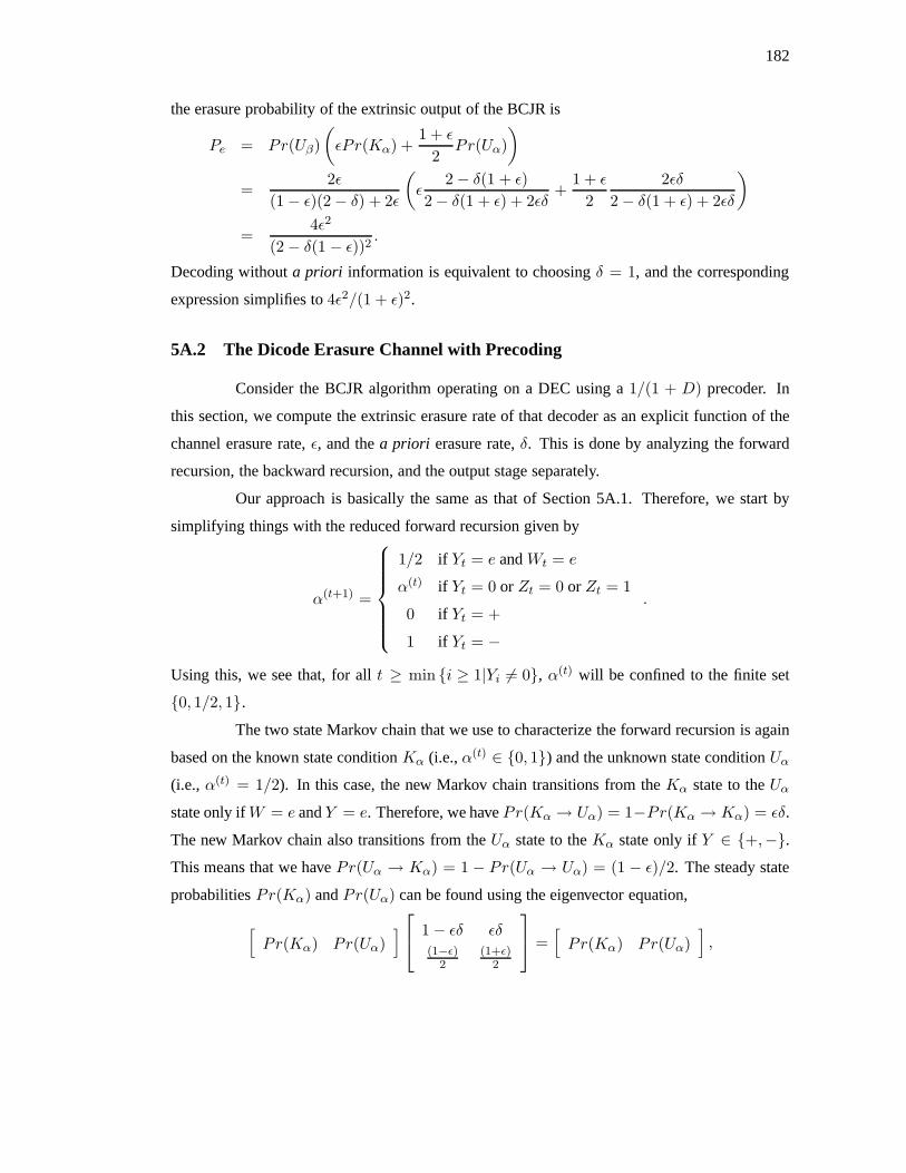
Our approach is basically the same as that of Section 5A.1. Therefore, we start by
simplifying things with the reduced forward recursion given by
α(t+1) =
1/2 if Yt = e andWt = e
α(t) if Yt = 0 orZt = 0 orZt = 1
0 if Yt = +
1 if Yt = −
.
Using this, we see that, for allt ≥ min {i ≥ 1|Yi 6= 0}, α(t) will be confined to the finite set
{0, 1/2, 1}.
The two state Markov chain that we use to characterize the forward recursion is again
based on the known state conditionKα (i.e.,α(t) ∈ {0, 1}) and the unknown state conditionUα
(i.e.,α(t) = 1/2). In this case, the new Markov chain transitions from theKα state to theUα
state only ifW = e andY = e. Therefore, we havePr(Kα → Uα) = 1−Pr(Kα → Kα) = εδ.
The new Markov chain also transitions from theUα state to theKα state only ifY ∈ {+,−}.
This means that we havePr(Uα → Kα) = 1 − Pr(Uα → Uα) = (1 − ε)/2. The steady state
probabilitiesPr(Kα) andPr(Uα) can be found using the eigenvector equation,[Pr(Kα) Pr(Uα)
] 1 − εδ εδ(1−ε)
2(1+ε)
2
=[Pr(Kα) Pr(Uα)
],
183
whose solution isPr(Kα) = 1 − Pr(Uα) = 1−ε1−ε+2εδ .
The precoded case is also simplified by the fact that the state diagram of the precoded
channel is such that time reversal is equivalent to negating the sign of the output. Therefore, the
statistics of the forward and backward recursions are identical andPr(Kβ) = 1 − Pr(Uβ) =
Pr(Kα).
Now, we consider the output stage of the BCJR algorithm for the precoded DEC. At
any point in the trellis, there are now four distinct possibilities for forward/backward state knowl-
edge:KαKβ, KαUβ , UαKβ, andUαUβ. At the extrinsic output of the decoder, the respective
erasure probability conditioned on each possibility is: 0,ε, ε, and ε. Therefore, the erasure
probability of the extrinsic output of the BCJR is
Pe = ε (1 − Pr(Kα)Pr(Kβ))
= ε
(1 − (1 − ε)2
(1 − ε+ 2εδ)2
)=
4ε2δ(1 − ε(1 − δ))(1 − ε(1 − 2δ))2
.
Again, decoding withouta priori information is equivalent to choosingδ = 1, and the corre-
sponding expression simplifies to4ε2/(1 + ε)2.
5B Joint Iterative Decoding DE for General Channels
While the initial steps of this analysis were focused on GECs, it is entirely possible
to write out the DE recursion, such as (5.3.1), for general message passing. Many of these
ideas were first introduced by Richardson and Urbanke in [13]. This recursion will track the
density function of the messages passed along a particular edge. In general, the messages will be
LLRs but most of this analysis does not depend on this. We will, however, make use of notation
based on using LLR messages. For example, we use∆∞ to denote the message implying perfect
knowledge of a “0” bit because, in the LLR domain, this message corresponds to a delta function
at infinity. Likewise, the message implying perfect knowledge of a “1” bit is denoted by∆−∞.
We also use∆0 to denote the message implying the complete lack of knowledge because, in the
LLR domain, this message corresponds to a delta function at zero.
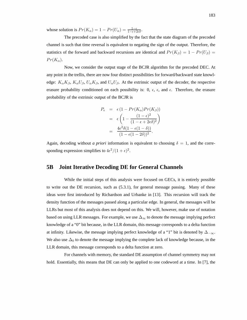
For channels with memory, the standard DE assumption of channel symmetry may not
hold. Essentially, this means that DE can only be applied to one codeword at a time. In [7], the
184
i.i.d. channel adaptor is introduced as a conceptual device which ensures the symmetry of any
channel. If the outer code is a linear code, then this approach is identical to choosing a random
coset and treating it as part of the channel. In this section, we use the i.i.d. channel adaptor
approach so that DE can be applied to all codewords simultaneously.
Let ⊗ be a commutative binary operator on message densities which represents the
message combining function for the bit nodes. For example, if the messages consist of LLRs,
then this operator will represent convolution because LLRs are added at the bit nodes. In this
case, the operator can be defined by noting thatR = P ⊗Q implies
R(x) =∫ ∞
−∞P (y)Q(x− y)dy.
Using the notation,
P⊗k = P ⊗ . . .⊗ P︸ ︷︷ ︸k times
,
for exponentials, we can now defineλ⊗(P ) =∑
ν≥1 λνP⊗ν−1 andL⊗(P ) =
∑ν≥1 LνP
⊗ν .
Let ⊕ be a commutative binary operator on message densities which represents the message
combining function for the check nodes. If min-sum decoding is used in the LLR domain,
then this operator can be defined by noting thatR = P ⊕ Q impliesR(x) = R+(x)U(x) +
R−(x)U(−x) +R0(x)∆0(x), where
R+(x) = P (x)∫ ∞
xQ(y)dy + P (−x)
∫ −x
−∞Q(−y)dy
R0 =∫ 0+
0−P (y)dy +
∫ 0+
0−Q(y)dy −
∫ 0+
0−P (y)Q(y)dy
R−(x) = P (x)∫ x
−∞Q(y)dy + P (−x)
∫ ∞
xQ(y)dy,
andU(x) is the unit step function. Using similar notation for operator exponentials, we also
defineρ⊕(P ) =∑
ν≥1 ρνP⊕ν−1. We also require that both of these operators be commutative
and associative with respect to scalar multiplication. This means that
cP ⊗Q = P ⊗ cQ = c(P ⊗Q),
and that the respective result holds for⊕.This allows us to apply the natural analogue of the
binomial theorem to show that
(aP ⊕ bQ)k =k∑
i=0
(k
i
)aibk−iP⊕i ⊕ P⊕k−i, (5B.1)
185
and that the respective result holds for⊗. We also note that the zero power gives the identity, so
P⊗0 = ∆0 andP⊕0 = ∆∞.
Our next assumption, known asdecoder symmetry, requires that the operators for the
bit and check nodes obey a few identities. The bit node operator must satisfyP ⊗ ∆0 = P ,
P ⊗ ∆∞ = ∆∞, andP ⊗ ∆−∞ = ∆−∞. This means, in some sense, that∆0 acts as an
identity and that∆∞ (and∆−∞) act as zero elements. The check node operator must satisfy
P ⊗ ∆∞ = P , P ⊗ ∆0 = ∆0, and the fact thatP = Q⊗ ∆−∞ impliesP (x) = Q(−x). This
means, in some sense, that∆∞ acts as the identity,∆−∞ acts as a negative identity, and∆0 acts
as the zero element. We note that most reasonable combining functions for the bit and check
nodes satisfy these properties.
Finally, we letF(P ) represent the mapping froma priori messages to extrinsic mes-
sages for the channel decoder. Using the same arguments used for (5.3.1), we can now write the
DE recursion as
Pi+1 = F(L⊗ (ρ⊕(Pi)
))⊗ λ⊗
(ρ⊕(Pi)
). (5B.2)
A sufficient condition for convergence can be defined by requiring, for example, that the hard
decision error probability is decreased by every iteration. The hard decision error probability
for a density is simply a projection of that density onto a scalar, and there are a variety of
such projections which can be used to define sufficient conditions for convergence. In the LLR
domain, entropy of the bit given the message is another projection that seems to work well.
Using the i.i.d. channel adaptor approach ensures that the expected value of the de-
coder trajectory does not depend on the codeword transmitted. Since the choice of the random
coset is absorbed into the channel, the all zero bit pattern still acts as a codeword and a fixed
point of the iteration. Therefore, the message density∆∞ is always a fixed point of the iteration
and we can discuss its stability. In the same manner as LDPC codes for memoryless channels
[13], we can expand this recursion in a series about∆∞ by lettingPi = (1 − ε)∆∞ + εQ. Our
only new assumption is that the channel mapping can be expanded about this density with
F ((1 − ε)∆∞ + εQ) = (1 − cF (Q)ε)F0 + cF (Q)εDF (Q) +O(ε2),
whereF0 is the perfect a priori channel LLR density,cF (Q) is a scalar valued function of a
density, andDF (Q) is a density valued function of a density. We note thatF0 can be estimated
in practice by simulating the channel decoder with perfecta priori information. The functions
186
cF (Q) andDF (Q) will usually depend in a complicated way onQ, but we can simplify things
by definingcF = supQ cF (Q). Using simulations, more accurate results may be possible by
estimatingcF (Q) andDF (Q) along a particular decoding trajectory.
Now, we can use (5B.1) to expand the operatorsρ⊕, λ⊗, andL⊗ around the density
(1 − ε)∆∞ + εQ. Forρ⊕, this gives
ρ⊕ ((1 − ε)∆∞ + εQ) =∑ν≥1
ρν
ν−1∑i=0
(ν − 1i
)(1 − ε)ν−1−iεi∆⊕ν−1−i
∞ ⊕Q⊗i
=∑ν≥1
ρν(1 − ε)ν−1∆∞ + ρ′(1)εQ+O(ε2),
because∑
ν≥1 ρν(ν − 1) = ρ′(1). Forλ⊗, this gives
λ⊗ ((1 − ε)∆∞ + εQ) =∑ν≥1
λν
ν−1∑i=0
(ν − 1i
)(1 − ε)ν−1−iεi∆⊗ν−1−i
∞ ⊗Q⊗i
= λ1∆0 +∑ν≥2
λν(1 − εν−1)∆∞ + λ2εQ+O(ε2).
ForL⊗, this gives
L⊗ ((1 − ε)∆∞ + εQ) =∑ν≥1
Lν
ν∑i=0
(ν
i
)(1 − ε)ν−iεi∆⊗ν−i
∞ ⊗Q⊗i
=∑ν≥1
Lν(1 − εν)∆∞ + aLλ1εQ+O(ε2),
becauseL1 = L′(0) = aLλ1.
Now, we can combine these expansions with (5B.2) to estimatePi+1 given thatPi =
(1 − ε)∆∞ + εQ. Working through the details shows thatPi+1 is given by((1 −O(ε))F0 + cFaLλ1ρ
′(1)εQ)⊗((1 −O(ε)) ∆∞ + λ1∆0 + λ2ρ
′(1)εQ)
+O(ε2),
which can be simplified to
(1 −O(ε)) ∆∞ + (1 −O(ε))λ1F0 + (1 −O(ε))λ2ρ′(1)εQ⊗ F0 + cFaLλ
21ρ
′(1)εQ. (5B.3)
Using this, we see that thef(0) = 0 condition for the GEC is very similar to theF0 = ∆∞ con-
dition for general channels. In this case, only the last term of (5B.3) matters and an approximate
187
stability condition is given bycFaLλ21ρ
′(1) < 1. If F0 6= ∆∞, then we must haveλ1 = 0 so
that the second term of (5B.3) vanishes. Whenλ1 = 0, only the third term of (5B.3) remains
and the stability condition is given by
λ2ρ′(1)
∫ ∞
−∞F0(x)e−x/2dx < 1.
We note that the integral in this equation follows from the stability condition derived for memo-
ryless channels in [13], and the symmetry ofF0(x) implied by the random coset assumption.
Bibliography
[1] D. Arnold and H. Loeliger. On the information rate of binary-input channels with memory.In Proc. IEEE Int. Conf. Commun., pages 2692–2695, Helsinki, Finland, June 2001.
[2] L. R. Bahl, J. Cocke, F. Jelinek, and J. Raviv. Optimal decoding of linear codes for mini-mizing symbol error rate.IEEE Trans. Inform. Theory, 20(2):284–287, March 1974.
[3] S. Chung, G. D. Forney, Jr., T. J. Richardson, and R. L. Urbanke. On the design of low-density parity-check codes within 0.0045 dB of the Shannon limit.IEEE Commun. Letters,5(2):58–60, Feb. 2001.
[4] C. Douillard, M. Jézéquel, C. Berrou, A. Picart, P. Didier, and A. Glavieux. Iterativecorrection of intersymbol interference: Turbo equalization.Eur. Trans. Telecom., 6(5):507–511, Sept. – Oct. 1995.
[5] R. G. Gallager. Low-Density Parity-Check Codes. The M.I.T. Press, Cambridge, MA,USA, 1963.
[6] J. Hou, P. H. Siegel, and L. B. Milstein. The performance analysis of low density parity-check codes on Rayleigh fading channels. InProc. 38th Annual Allerton Conf. on Com-mun., Control, and Comp., volume 1, pages 266–275, Monticello, IL, USA, Oct. 2000.
[7] J. Hou, P. H. Siegel, L. B. Milstein, and H. D. Pfister. Multilevel coding with low-densityparity-check component codes. InProc. IEEE Global Telecom. Conf., pages 1016–1020,San Antonio, Texas, USA, Nov. 2001.
[8] A. Kavcic, X. Ma, and M. Mitzenmacher. Binary intersymbol interference channels: Gal-lager codes, density evolution and code performance bounds. submitted toIEEE Trans.Inform. Theory, 2001.
[9] B. M. Kurkoski, P. H. Siegel, and J. K. Wolf. Joint message-passing decoding of LDPCcodes and partial-response channels.IEEE Trans. Inform. Theory, 48(6):1410–1422, June2002.
188
[10] M. G. Luby, M. Mitzenmacher, and M. A. Shokrollahi. Analysis of random processes viaand-or tree evaluation. InSODA: ACM-SIAM Symposium on Discrete Algorithms, pages364–373, Jan. 1998.
[11] M. G. Luby, M. Mitzenmacher, M. A. Shokrollahi, D. A. Spielman, and V. Stemann. Prac-tical loss-resilient codes. InProc. of the 29th Annual ACM Symp. on Theory of Comp.,pages 150–159, 1997.
[12] H. D. Pfister, J. B. Soriaga, and P. H. Siegel. On the achievable information rates of finitestate ISI channels. InProc. IEEE Global Telecom. Conf., pages 2992–2996, San Antonio,Texas, USA, Nov. 2001.
[13] T. J. Richardson, M. A. Shokrollahi, and R. L. Urbanke. Design of capacity-approachingirregular low-density parity-check codes.IEEE Trans. Inform. Theory, 27(1):619–637, Feb.2001.
[14] V. Sharma and S. K. Singh. Entropy and channel capacity in the regenerative setup withapplications to Markov channels. InProc. IEEE Int. Symp. Information Theory, page 283,Washington, DC, USA, June 2001.
[15] M. A. Shokrollahi. New sequences of linear time erasure codes approaching the channelcapacity. InApplicable Algebra in Eng., Commun. Comp., pages 65–76, 1999.
[16] M. A. Shokrollahi. Capacity-achieving sequences. InCodes, Systems, and GraphicalModels, volume 123 ofthe IMA Vol. in Math. and its Appl., pages 153–166. Springer,2001.
[17] S. ten Brink. Rate one-half code for approaching the Shannon limit by 0.1 dB.ElectronicLetters, 36(15):1293–1294, July 2000.
[18] S. ten Brink. Convergence behavior of iteratively decoded parallel concatenated codes.IEEE Trans. Commun., 49(10):1727–1737, Oct. 2001.
[19] S. ten Brink. Exploiting the chain rule of mutual information for the design of iterativedecoding schemes. InProc. 39th Annual Allerton Conf. on Commun., Control, and Comp.,Oct. 2001.
[20] R. Urbanke. Iterative coding systems. http://www.calit2.net/events/2001/courses/ics.pdf,Aug. 2001.
[21] N. Varnica and A. Kavcic. Optimized LDPC codes for partial response channels. InProc.IEEE Int. Symp. Information Theory, page 197, Lausanne, Switzerland, June 2002. IEEE.
Recommended