61
MATHEMATICAL MODELLING RELATED TO THE
INTERNATIONAL GEOSPHERE-BIOSHPERE PROGRAM AT
THE CENTRE FOR RESOURCE AND ENVIRONMENTAL STUDIES
INTRODUCTION
John A. Taylor, Anthony J . .lakeman,
Michael S. Common and Michael F. Hutchinson
The aim of the research in CRES is to help identify and provide balanced analyses
of resource and environmental policy problems, thereby facilitating the resolution of policy
options. There has recently been a shift in emphasis away from analysis of specific national
problems that can be treated in a short time frame, and hence mostly with existing
knowledge and data. Research is now directed towards the construction of decision support
tools for long-term acquisition of fundamental information of general use to a common core
of resource and environmental problems of national and global concern. At the same time
flexibility has been retained to consider important topical problems as they arise on the
public policy agenda; attention to these motivates the long-term research program and
makes it more robust.
The basic premise in the Centre's long-term research direction is that there are
large gaps in the knowledge base for treating many resource and environmental problems,
including impact assessment of the greenhouse effect. Research and decision support tools
are required to address these gaps and in general they are intended to be climate sensitive
and their predictions robust to changes in climatic-related inputs. Examples of the tools in
continual development are geographic information systems to house essential spatial and
temporal information in a systematic and accessible form and generic lmodels', such as
62
those for environmental flow and solute transport, which can interpolate, extrapolate or
predict with this information those quantities of prescriptive interest.
The form of any given model is highly dependent on the type of problem for which
it is intended and the nature of the "",i<>rlup and data available for its construction and
use. Many are physically based mathematical models often containing a stochastic element
to account for uncertainty, but the models may also be more qualitative, particularly when
the problem is set in a social science context. Exercises involving the construction,
calibration and validation of models is called 'system identification', while exercises
involving the running of models with inputs and already calibrated parameter values is
called 'system simulation'. Most of the research time is spent on system identification.
In the following sections, some specific information and references are provided
which illustrate the Centre's research effort and success in developing tools for climate
impact assessment.
L STREAM HYDROGRAPH SEPARATION
The unit hydrograph is the streamflow response of a catchment to a unit of rainfall
excess, excess being that rainfall not lost through evapotranspiration. It is a fundamental
catchment-scale property reflected in the streamflow. Jakeman, Littlewood and Whitehead
[1, 2] have developed a conceptual model and procedure for characterising the unit
hydrograph and for separating the quickflow response, which includes overland flow, and
the slowflow response, which includes subsurface flows, to stream. Uses of the separation
include the construction of baseflow indices for water quality potential and for inferring
moisture content in the catchment. The approach has several attractive features which its
competitors lack. It can be used for small catchments from short time series of rainfall,
temperature and streamflow records with sampling intervals as short as one hour. Base
flow separation is an integral component of model identification and unlike traditional
methods, is related dynamically to the rainfall. All the available rainfall-streamflow data
63
can be used, avoiding the need to arbitrarily select clean, single-peaked events for analysis
and contributing to model parameters with better definitions.
2. PREDICTING ENVIRONMENTAL EXTREMES
Extremes such as air pollutant and water pollutant concentrations which occur for
short periods in an annual series are difficult to predict. Jakeman and Taylor [3] report
details of a hybrid modelling concept developed in CRES to predict pollutant extremes
from process-based model predictions of annual mean concentrations and a statifltical
appreciation of the parametric form of the frequency distribution of pollutant
concentrations. The approach has been used in several studies to predict air pollutant
concentrations from vehicle emissions and industrial sources (eg. Jakeman, Simpson and
Taylor [4]; Jakeman and Taylor [5]; Jakeman and Simpson [6, 7] and Taylor, Simpson and
Jakeman [8, 9]). More recently, it has been applied to the prediction of water quality
extremes (Jakeman et al. [10]) and in particular stream acidity variables.
3. GROUNDWATER SYSTEM IDENTIFICATION VIA INDIRECT METHODS
AND RANDOM FIELD REPRESENTATION OF UNKNOWN PARAMETERS
The problem of groundwater system identification is an inverse problem in which
unknown aquifer parameters (such as hydraulic conductivity) in the groundwater flow
equation are inferred from data on piezometric pressure. Because data on such groundwater
systems are typically scarce and unreliable, care must be taken in inferring aquifer
parameters (Dietrich et al. [11]). Work is in progress on a random field representation of
hydraulic conductivity that depends only on a few parameters describing essentially the
small- and large-scale features of the porous matrix through which water flows. Parameter
inference from water pressure data is then obtained via non-linear optimisation to best fit
64
the available data. Results of this work are to be used for a paper (Dietrich [12]) at an
international conference on groundwater modelling at The Hague in September 1990.
Work has also commenced on reducing the operation count associated with solving
the groundwater flow equation in steady and unsteady state for those cases where the
hydraulic conductivity is smooth. Finite element discretisation is used. Among others, an
application of such an algorithm is the use of Monte Carlo type procedures for parameter
identification along the lines of a Generalised Sensitivity Analysis. An example of the latter
procedure is given in Jakeman et aL [13].
Among the set of parameters that need to be measured to model climatic effects on
an aquifer, recharge is possibly the most important and the one least known. In another
CRES project, the aim is to estimate effective recharge from head measurements and prior
information through an inverse procedure based on a maximum likelihood approach
stabilised by imposing constraints on the noise structure.
4. MATHEMATICAL MODELLING OF UPCONING AND SEAWATER
INTRUSION
Management of groundwater resources in coastal areas and isolated islands, where
groundwater is the source of water and the aquifers are subject to intrusion of
seawater, is a delicate problem. The extent of this intrusion depends on many factors,
including aquifer geometry and properties, abstraction rate and depth, recharge rate and
distance of pumping bores from the coastline. Some of these factors can be affected by
changes in climate. Sophisticated tools are required to quantify the effect of these factors.
In this context, the ability of a two~imensional mathematical model named
SUTRA, developed by the US Geological Survey in 1984, has been tested to simulate a
critical case in Nauru Island in the Pacific Ocean (Ghassemi, Jakeman and Jacobson
[14]).The methodology proved to be very successful in quantifying the sensitivity of the
aquifer to the type and level of abstraction and could be applied to coastal aquifers of
65
Australia. Data collection is in progress to identify the most suitable coastal aquifers in
Australia for the simulation approach. In the meantime, the performance of a
three-dimensional model named HST3D, developed by the US Geological Survey in 1987,
is under investigation. If tests prove successful, new opportunities will arise for more
accurate simulation of these problems.
5. CLIMATE CHANGE AND GROUNDWATER RESOURCES OF AUSTRALIA
Recent statistics published by the Department of Primary Industry and Energy
show that the annual runoff of the continent is about 397 billion cubic metres out of which
98.1 billion are divertible. Divertible fresh and marginally fresh groundwater resources with
salinity less than 1500 mgjL comprise about 22 billion cubic metres.
The annual water use in Australia is 15 billion cubic metres of which 70 per cent is
used for irrigation, 21 per cent is used for the domestic and industrial sectors and 9 per
cent for other purposes.
As a source of water supply, surface water contributes 82 per cent and groundwater
the remaining 18 per cent. Although the contribution of groundwater to total water use
seems relatively small, many areas, especially in arid and semi-arid, and even temperate
and tropical zones, are totally or at least heavily dependent on groundwater as a source of
water supply. While the country enjoys a substantial volume of undeveloped surface and
ground water resources per head of population, these potential sources are not evenly
distributed and in many cases they are far from the major sources of demand.
To complicate this assessment, there is some evidence from climatological studies
that the pattern of Australian rainfall changed from the period 1913--45 to the period
1946-73. Rainfall increased in many areas, an exception being the southwest of Western
A ustralia where rainfall decreased. There was a southward shift in the region of
summer-dominated rainfall. Predicted climatic changes due to the accrual of greenhouse
66
gases from fossil fuel burning and other anthropogenic sources means that these trends may
continue.
Climatic change of this nature will have major effects on the groundwater resources
of the continent. CRES analysis by Ghassemi, Jacobson and Jakeman [25] argues that the
effects will be beneficial in the arid and semi-arid areas and in areas where aquifers are
under stress due to overdevelopment, such as many of the alluvial aquifers of Queensland
and New South Wales. Effects will be detrimental in some other important areas such as
the Perth and Murray Basins. In addition, rises in sea-level will increase the intrusion of
seawater in coastal aquifers and will reduce the sustainable yield of freshwater in aquifers
such as the Swan Coastal Plain (WA), Botany Bay and Tomago Sands (NSW), Western
Port (Vic), Burdekin Delta (Qld) and Seven Mile Beach (Tas).
6. CLIMATE MODELLING
The greenhouse effect and the potential for climate change have attracted
considerable attention from the Australian scientific community and the Australian public
over the few years (Taylor [15]). This interest has been prompted by the concern for
the substantial impacts of climate warming on Australia and the world. In order to address
these concerns and to coordinate research within the Centre, a versatile, modular and
well-documented climate model was obtained from the United States National Center for
Atmospheric Research (NCAR). In conjunction with the ANU supercomputer facility, the
Community Climate Model (CCMl) code is being converted to run on the AND Fujitsu
VP-IOO supercomputer. The code conversion will be completed in 1990. The model has
been developed and used successfully by the United States university research community
to conduct many diverse experiments which were seen to relate to each other when
performed with the saine model. The CCMl has led to much constructive dialogue and
collaboration between experts in several disciplines. In view of the successful application of
the CCMl in the United States and the large body of documentation of the model and
67
large number of scientific studies conducted with it, it is intended that the code will be
made available to the Australian scientific community through the ANU Supercomputer
Facility external grants scheme and through collaboration with ANU scientists.
7. GLOBAL TRACER TRANSPORT MODELLING
A major impediment to our understanding of the biogeochemical cycles of
atmospheric trace gases that cause climate change has been the lack of high resolution
three-dimensional global circulation models which can be used to identify the sources and
sinks, including atmospheric chemistry, of these trace gases (Taylor [16]). In the past, even
low resolution three-dimensional models have placed enormous computational demands on
supercomputers. This project has involved the development of a computationally efficient
high-resolution simulation model for atmospheric transport and chemistry with
parameterised interactions between the oceans and the biosphere (Taylor [16, 17, 18, 19];
Taylor et al. [20]).
The basic approach of the stochastic Lagrangian model is to divide the atmosphere
into 100 000 air parcels of equal mass. Trajectories for these air parcels are calculated using
wind speed data derived from observed wind fields obtained from the European Centre for
Medium Range Weather Forecasting. While the simulated air parcels are being transported
around the globe they can exchange chemical species with the oceans, the biosphere and
one another and receive industrial emissions of greenhouse gases.
An important aspect of this approach is the very high computational speed
achievable on modern supercomputers. One-year model integrations are now achievable in
a few minutes on supercomputers where once this would have taken hours. Model results,
consisting of predicted atmospheric concentrations are currently analysed and displayed as
colour animations on a Sun workstation at CRES.
68
8. GREENHOUSE GASES: CARBON DIOXIDE
The determination of the fluxes associated with the sources and sinks of CO2
remains an important problem in the study of the global carbon cycle. The difficulties
associated with obtaining precise quantitative estimates of the biospheric and oceanic
exchanges of C02 with the atmosphere by direct measurement or from theoretical
considerations has led a number of researchers to attempt to infer from modelling studies,
employing the best available transport a set of fluxes consistent with the observations
of CO2 in the atmosphere.
Using the three-dimensional stochastic Lagrangian model and incorporating
available estimates of the global distribution of anthropogenic C02 emissions and
biospheric and oceanic exchanges of C02) a model of the global distribution of atmospheric
concentration was constructed (Taylor [16]). Model predictions were then compared
with available observations.
From the model studies it was found that a flux from the oceans of 1.6 gigatonnes of
carbon and biospheric growing season net flux of 6.5 gigatonnes were consistent with
available observations. However, the assumption that large amounts of C02 were
transported from the northern hemisphere to the southern hemisphere and then absorbed
by the southern oceans below 45" S could not be supported.
This observation has important climatic implications. If the oceans are not
absorbing as much C02 as previously thought, then the biosphere must be absorbing a
large amount of C02. It is unlikely that the biosphere will be able to continually remove
increasing anthropogenic releases of C02. This may lead to an increase in the rate of
climate change. Alternatively, a different model of the spatial distribution of the uptake of
CO2 by the oceans may also explain the observed C02 concentrations. It was also found
that above 60' N the predicted seasonal cycle associated with the biospheric release of CO 2
was inconsistent with the observed seasonal cycle. This may mean that carbon storage is
occurring at these latitudes and that the model of C02 respiration needs to be revised.
69
9. GREENHOUSE GASES: METHANE AND METHYL CHLOROFORM
The sources and sinks of methane and methyl chloroform have also been
investigated by incorporating models for their sources and sinks into the global tracer
transport model (Taylor et aL [20]). Results indicated that available estimates of methyl
chloroform emissions for the period 1981-84 were underestimated by 10-20 per cent or that
the hydroxyl radical concentration had declined by a similar amount. Results of recent
assessments of the release of methyl chloroform published after the completion of this study
have confirmed the predicted releases of methyl chloroform. The much larger releases of
methyl chloroform predicted by the model indicate that the release of this greenhouse gas is
continuing to grow at a rapid rate.
Methane is a key chemical in the chemistry of both the troposphere and the
stratosphere. Two source functions for the spatial and temporal distribution of the flux of
methane to the atmosphere were developed. The first model was based on the assumption
that methane is emitted from the biosphere as a proportion of net primary productivity
(NPP). This model generated an estimate of the methane source term of 623 Tg CH4,
giving an atmospheric lifetime for methane of 8.3 years. The excellent performance of the
NPP model for generating estimates of methane fluxes indicates that anaerobic odixation
closely follows the seasonal cycle of photosynthesis. The results also indicate that if
methane fluxes are proportional to NPP, then any C02 fertilisation effect will lead to
increasing releases of methane, further accelerating climate change produced by the
greenhouse effect.
The second model identjfied source regions for methane from rice paddies, wetlands,
enteric (intestinal) fermentation, termites and burning of biomass, based on
high-resolution land use data. This methane source distribution resulted in an estimate of
the global total methane source of 611 Tg CH4, giving an atmospheric lifetime for methane
of about 8.5 years. The most significant difference between the two models were predictions
of methane fluxes over China and Southeast Asia, the location of most of the world's rice
paddies.

70
HI. ACCOUNTING FOR AUSTRALIAN CARBON mOXIDE EMISSIONS
If policies to abate global warming are to be a major focus will be carbon
dioxide emissions arising in fuel combustion. The proper analysis of policy options in this
context will require an accounting of the sources of such emissions in terms of the ultimate
purpose of the combustion, rather than in terms of institutional and structural location. It
is not enough to know, for example, that x per cent of emissions arise in
generation. It is also necessary to know what electricity is used for, and to allocate the x
per cent over those uses, This section of the paper briefly describes a methodology for such
an end use accounting for carbon dioxide emissions, and reports results for Australia. The
ana.lytical potential of the methodology is also indicated. A fuller treatment of each of
these matters is given in Common and Salma [21].
The objective is an exhaustive allocation of total emissions across a
commodity /industry disaggregation of deliveries to final demand, which consists of
consumption by households and government, capital and stock accumulation, and exports,
These are regarded as the end purposes of economic activity. The appropriate methodology
is input-output analysis. With
y
x
A
n
we have
(1)
a vector of final demand requirements commodity,
a vector of gross output levels by industry,
a matrix of technological coefficients for the industrial input requirements of
industries for unit activity levels, and
number of commodities and industries,
x = (I_A)-l Y = Ly
giving the relationships between gross output levels and final demand deliveries, where the
former comprise the latter plus production of inputs to other industries. Then with
C a matrix of coefficients for primary energy inputs per unit of gross output by
industry,
F
e
we have
(2)
and
(3)
71
a matrix of coefficients for primary energy inputs per unit of delivery to final
demand,
a vector of coefficients for carbon dioxide release per energy unit of fuel
burned,
T = e ( Cx + Fy) = e ( CLy + Fy) = e ( CL + F) y = ty
Z= t*y
where T is total emissions, t is a vector the n elements of which are emissions per unit of
commodity delivery to final demand, z is a vector of the total emissions attributabte to
each commodity, and t* is and n x n matrix with t along its diagonal and zeros elsewhere.
Implementation of this methodology for Australian carbon dioxide emissions
requires data for e, C and F, and for L (known as the Leontief inverse) and y. The source
for Land y is input-output data. At the time of writing the most recent available was that
for 1982/3, in ABS [22], and it is to that year that the results to follow relate. For reasons
discussed in Common and Salma [21] it was necessary to modify the commodity/industry
classifications used in ABS [22], and to set n equal to 27. This meant calculating L from
reconstructed flow data rather than using the published table for this matrix. The elements
of the matrices C and F were calculated from energy data for 1982/3 given in BRE [23]. Six
primary fuels - black and brown coal, wood, bagasse, natural gas and oil - were used, so
that C and Fare 6 x 27 matrices. The other primary fuels are solar and hydro, which give
rise to no emissions, and uranium which additionally is not used in Australia. The vector e
then has six elements, values for which were taken from AlP [24].
On this basis, total fuel combustion emissions in Australia for 1982/3 were
calculated as 257340 kT. The corresponding figure for 1988/9, which can be derived
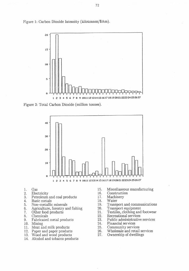
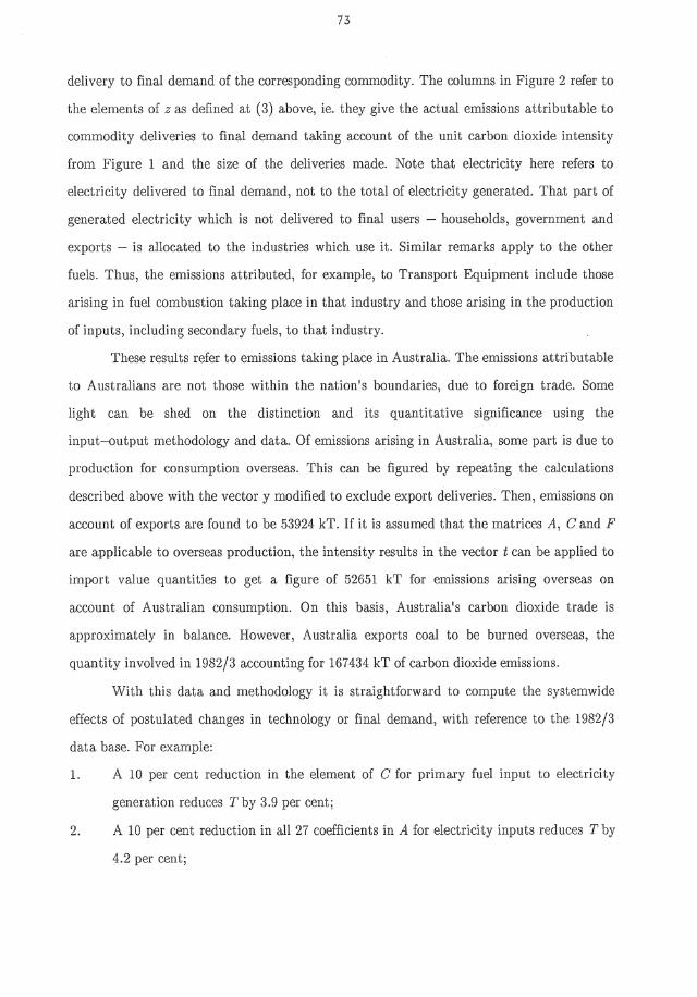
without using the input-output data, is 318258 million kT. Figures 1 and 2 here give
results obtainable only by way of the input-output approach. In Figure 1 the elements of t
as defined by (2) above are shown, ie. the height of a column gives the amount by which
total emissions would increase (decrease) for a unit ($A million) increase (decrease) in the
'72
Figure 1: Carbon Dioxide Intensity (kilotonnes/$Am).
15
Figure 2: Total Carbon Dioxide (million tonnes).
39
19
1 2: :3 'I :5 67'S 9 UH1!2%314151617'H11928212223242S2621
1. Gas 15, Miscellaneous manufacturing 2. Electricity 16. Construction 3. Petroleum and coal products 17. Machinery 4. Basic metals 18. Water 5. Non-metallic minerals 19. Transport and communications 6. Agriculture, forestry and fishing 7. Other food products
20. Transport equipment 21. Textiles,elothing and footwear
8. Chemicals 22. Recreational services 9. Fabricated metal products 23. Public administrative services 10. Mining 24. Financial services 11. Meat and milk products 25. Community services 12. Paper and paper products 26. Wholesale and retail services 13. Wood and wood products 27. Ownership of dwellings 14. Alcohol and tobacco products
73
delivery to final demand of the corresponding commodity. The columns in Figure 2 refer to
the elements of z as defined at (3) above, ie. they give the actual emissions attributable to
commodity deliveries to final demand taking account of the unit carbon dioxide intensity
from Figure 1 and the size of the deliveries made. Note that electricity here refers to
electricity delivered to final demand, not to the total of electricity generated. That part of
generated electricity which is not delivered to final users - households, government and
exports - is allocated to the industries which use it. Similar remarks apply to the other
fuels. Thus, the emissions attributed, for example, to Transport Equipment include those
arising in fuel combustion taking place in that industry and those arising in the production
of inputs, including secondary fuels, to that industry.
These results refer to emissions taking place in Australia. The emissions attributable
to Australians are not those within the nation's boundaries, due to foreign trade. Some
light can be shed on the distinction and its quantitative significance using the
input-output methodology and data. Of emissions arising in Australia, some part is due to
production for consumption overseas. This can be figured by repeating the calculations
described above with the vector y modified to exclude export deliveries. Then, emissions on
account of exports are foun-d to be 53924 kT. If it is assumed that the matrices A, C and F
are applicable to overseas production, the intensity results in the vector t can be applied to
import value quantities to get a figure of 52651 kT for emissions arising overseas on
account of Australian consumption. On this basis, Australia's carbon dioxide trade is
approximately in balance. However, Australia exports coal to be burned overseas, the
quantity involved in 1982/3 accounting for 167434 kT of carbon dioxide emissions.
With this data and methodology it is straightforward to compute the systemwide
effects of postulated changes in technology or final demand, with reference to the 1982/3
data base. For example:
1. A 10 per cent reduction in the element of C for primary fuel input to electricity
generation reduces T by 3.9 per cent;
2. A 10 per cent reduction in all 27 coefficients in A for electricity inputs reduces T by
4.2 per cent;
74
30 A 10 per cent reduction in all 27 coefficients in A for basic metal inputs reduces T
by 1.4 per cent;
4. A 10 per cent reduction in the final demand for electricity reduces T 1.6 per cent.
11. SPATIAL AND TEMPORAL ANALYSIS OF ENVIRONMENTAL DATA FOR
GREENHOUSE SCENARIO EVALUATION
Current of greenhouse gas induced climate trends are largely based on the
of general circulation models While this has undoubtedly
made a major contribution to our understanding of the dynamics of the earth's
the current spatial resolution of GCMs of at best a few hundred kilometres is
recognised to be a serious Reliable simulation of ocean and
is heavily dependent on a detailed of ocean and
surface as well as having an accurate representation of the hydrological
properties of the earth's surface, Computational as well as limits on the
of detailed surface and have meant that GCMs have
very little to say about
kilometres. However, it is
with
change,
regional climate changes at spatial resolutions of a few
at this relatively fine resolution that useful conclusions can
to the development of strategies for coping with climate
Generic (process based) spatial and temporal techniques are being
developed at the Centre for Resource and Environmental Studies, These techniques impact
in a number of ways on the problem of generating regional greenhouse scenarios, Principal
contributions are:
(i) procedures for accurately describing the spatial distributions of. both current and
projected climate;
the development of process based models of the dependence on climate of both
natural and human related biological activity.
75
Aspects of these contributions are now briefly described.
11.1 SP ATIAL ANALYSIS OF CLIMATE
Thin plate smoothing splines have been applied to Australia wide, terrain
dependent, interpolation of climate (Hutchinson, [26]). The basic interpolation technique
has been described by Wahba and Wendelberger [27) and, in an enhanced form suitable for
larger data sets, by Bates and Wahba [28], Elden [29) and Hutchinson [30). Thin plate
smoothing splines determine an optimal balance between data fidelity and surface
smoothness by minimizing the generalized cross validation, a reliable measure of the true
predictive error of the fitted surface. A simply calculated stochastic estimator of the trace
of the influence matrix associated with thin plate smoothing splines has also been recently
described by Hutchinson [45]. This estimator is particularly useful for calculating the
generalized cross validation when analyzing very large data sets.
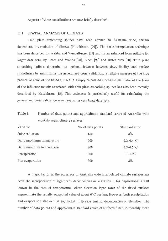
Table 1: Number of data points and approximate standard errors of Australia wide
monthly mean climate surfaces.
Variable No. of data points
Solar radiation 150
Daily maximum temperature 900
Daily minimum temperature
Precipitation
Pan evaporation
900
10000
300
Standard error
3%
0.2-0.4" C
0.3-0.5' C
10-15%
5%
A major factor in the accurracy of Australia wide interpolated climate surfaces has
been the incorporation of significant dependencies on elevation. This dependence is well
known in the case of temperature, where elevation lapse rates of the fitted surfaces
approximate the usually accpepted value of about 6" C per km. However, both precipitation
and evaporation also exhibit significant, if less systematic, dependencies on elevation. The
number of data points and approximate standard errors of surfaces fitted to monthly mean
76
values of solar daily maximum and minimum temperature, precipitation and pan
evaporation are shown in Table 1. These variables are the principal climatic determinants
of growth.
11.2 DIGITAL ELEVATION MODELLING FOR CLIMATE AND HYDROLOGIC
ANALYSIS
Terrain a dominant role in deiGermlmrlg the ~"~k'V~' and environmental
characteristics of a In order to make lise of the on elevation
regular exhibited the climate surfaces described
elevation models from surface elevation contour line data and
stream line data has been Hutchinson [31, The
three principal innovations. The first is an efficient multi-grid, finite
difference interpolation many thousands of data
to a user The second is a enforcement
which removes spurious sinks or pits in the fitted elevation grid, in
of the fact that sinks are normally quite rare in nature. The third is an
algorithm which calculates ridge lines and stream lines from of locally
maximum curvature on data contour lines.
The drainage enforcement algorithm in particular has been found to significantly
increase the power of the technique, when data are relatively
sparse. It also facilitates the use of the calculated digital elevation models in hydrological
process studies which depend in part on the calculation of contributing catchment areas
(Abbot et [33]; Moore et aL, [34]. This is also of significance in modelling soil moisture
regimes which strongly moderate plant growth, especially in the semi-arid conditions
which prevail over much of Australia.
11.3 CONSEQUENCES FOR GREENHOUSE SCENARIO ANALYSIS
The digital elevation modelling has been applied to the calculation of a
elevation model for Australia (Hutchinson and [35]). The resolution of this
77
model is 0.025 deg lat/long (about 2.5 km). When combined with the elevation dependent
climate surfaces described above, this yields accurate, continent wide, descriptions of the
spatial distribution of the current climate. By systematically perturbing these distributions .
according to zonally averaged predictions afforded by general circulation models,
preliminary assessments of the effects of climate change on agriculture have been made by
Pittock and Nix [36] and Hennessy and Pittock [37]. Projected spatial displacements of
climate also have major implications for the conservation of plant and animal species which
currently inhabit environments of limited areal extent. The BIOCLIM program described
by Nix [38] can be used to match occurrences of native flora and fauna to existing climate
in order to generate likely consequences on the distribution of native plant and an.imal
species under changed climate conditions.
11.4 PROCESS BASED STOCHASTIC WEATHER MODELS
In order to address temporal variability in a more realistic fashion than that allowed
by long term monthly climate means, simple process based stochastic weather models are
being developed. An important aspect of this work is its attempt to incorporate in the
stochastic model key physical interactions between the weather variables. Thus a model in
continuous time is being developed which is based on modelling the occurrence of cloud,
since cloud moderates rates of heating during the day and rates of cooling at night. Cloud
occurrence is also a necessary precondition for the occurrence of precipitation. The goal of
this approach is to develop a weather model with a relatively small number of physically
interpretable parameters which can be robustly determined from limited climate statistics
and which can be realistically perturbed in response to projected climate changes. The
physical basis for the model means that its validity should be relatively unaffected by these
changes.
The first step in this work has been the development of a stochastic model for
precipitation occurrence based on a continuous Markov process (Hutchinson, [39]). The
model appears to be superior to existing point rainfall models based on Poisson cluster
processes in terms of its physical interpretability, its ability to match observed statistics
78
and its mathematical tractability. Moreover, the model is amenable to further
enhancements such as the simulation of cloud occurrence. Related work on the
development of physically based stochastic models for temperature and solar radiation is
carried out by Guenni et aL and Chia [41] respectively. An important aspect of
this work is model calibration. A technique for robust calibration of seasonally varying
stochastic weather models using periodic splines has been described
Hutchinson Unlike methods based on Fourier the coefficients of polynomial
are well conditioned in terms of the data Boor, which makes them well
suited to
Stochastic models can be used to information on of the
future climate such as the of extreme events floods,
Calculations of these probabilities
limited on of
repeated simulation of a general circulation model are
expense. Moreover, a stochastic weather model can be
used to drive process based crop growth IHU'UC1.n. such as that described Nix [44],
in order to generate information on both the amount and variability of agricultural output.
This technique is vital to the assessment of consequences for agricultural production and
the development of appropriate strategies to maintain if not improve agricultural output
under a changed climate.
REFERENCES
[1] JAKEMAN, A.J., LITTLEWOOD, LG. and WHITEHEAD, P.G., (1990)
Computation of the instantaneous unit hydrograph and identifiable component
flows with application to two small upland catchments. J. Hydrology (in press).
[2] JAKEMAN, A.J., LITTLEWOOD, LG. and WHITEHEAD, P.G., (1990)
Catchment-scale rainfall-runoff event modelling and dynamic hydograph
separation. Proceedings Natural Environment Research Council and Institute for
Mathematics and Its Applications Conference on Computer Modelling in the
Environmental Sciences, Keyworth, UK. 10-11 April.
79
[3] JAKEMAN, A.J. and TAYLOR, J.A. (1989) Identification, estimation and
simulation of frequency distributions of pollutant concentrations for air quality
management. Chapter 4 in Library oj Environmental Control Technology, Gulf
Publishing, Houston, Cherernisinoff, P., (ed.) 2, 135-158.
[4] JAKEMAN, A.J., SIMPSON, R.W. and TAYLOR, J.A., (1988) Modelling
distributions of air pollutant concentrations. Part III: the hybrid
deterministic-statistical distribution approach. Atmospheric Environment 22,
163-174.
[.5] JAKEMAN, A.J. and TAYLOR, JA, (1985) A hybrid ATDL-gamma
distribution model for predicting urban area source acid gas concentration.
Atmospheric Environment 19, 1959-1967.
[6] JAKEMAN, A.J., and SIMPSON, R.W., (1985) Assessment of air quality
impacts from an elevated point source. Journal Environmental Management
20,63-72.
[7] JAKEMAN, A.J. and SIMPSON, R.W., (1987) Air quality and resource
[8]
[9]
a risk assessment in the Hunter Region in Australia. CRES
Monograph, Centre for Resource and Environmental Studies, Australian
National University.
TAYLOR, J.A., SIMPSON, R.W. and JAKEMAN, (1985) A hybrid
model for predicting the distribution of pollutants dispersed from line sources.
Science of the Total Environment 46,191-213.
TAYLOR, SIMPSON, R.W. a.nd JAKEMAN, (1987) A hybrid
model for predicting the distribution of sulphur dioxide concentrations observed
near elevated point sources. Modelling 36, 269-296.
[10J JAKEMAN, WHITEHEAD, ROBSON, A., JENKINS, A. a.nd
TA YLOR, J (1990) A method for predicting the extremes of stream acidity
and other water quality varibales. J. Hydrology (in press).
[11] DIETRICH, C.R., NEWSAM, G.N., ANDERSSEN, R.S., JAKEMAN, A.J.
and GHASSEMI, F, (1990) A practical account of instabilities in identification
problems in groundwater systems. Australian Journal of
Geophysics (in press).
and
80
[12] DIETRICH, C.R., (1990) Optimum selection of basis functions for ill-posed
inverse problems. IAHS International Conference on Model Calibration and
Reliability in Groundwater Systems, The Hague, 3--6 September, 1990.
[13] JAKEMAN, GHASSEMI, F., DIETRICH, C.R., MUSGROVE, T.J. and
[JA]
WHITEHEAD, P.G. Calibration and reliability of an aquifer system
model using generalised analysis. IAHS International Conference on
Model Calibration and Reliability in Groundwater Systems, The Hague, 3--6
September 1990.
F.,
modelling of sea
press) .
Mathematical
Processes
[15] TAYLOR, J.A., The effect and climate change: an Australian
perspective. CRES Working Paper, Australian National University.
[16] TAYLOR, (1989) A stochastic Lagrangian atmospheric transport model to
determine global C02 sources and sinks. A preliminary discussion. Tellus 41B,
272-285.
[17] TAYLOR,J (1990) New approaches to modelling the global distribution of
trace gases in the troposphere. Mathe.matics and Computers in Simulation.
[18] TAYLOR, J.A., (1990) A 3-dimensional global tropospheric transport and
modeL the 10th International Conference the Clean
Air Society of Australia and New Zealand.
[19] TAYLOR, J.A., (1990) A model of sources and sinks of trace gases important to
climatic change. Proceedings Natural Environment Research Council and
Institute for Mathematics and Its Applications Conference on Computer
Modelling in the Environmental Sciences, Keyworth, UK. 10-11 April.
[20] TAYLOR, J.A., BRASSEUR, G., ZIMMERMAN, P. and CICERONE, R.,
(1990) A study of the sources and sinks of methane using a global 3-d
Lagrangian tropospheric tracer transport modeL J. Geophys. Res. (To appear).
[21] COMMON, M. and SALMA, U., (1990) Accounting for Australian Cal'bon
Dioxide DII,\'t!;!j'UJ/,!j. Centre for Resource and Environmental Studies, ANU.
[26]
[27]
[28]
[30]
81
(1988) Australian National Accounts: Tables 1981-2 and
AJP,
Australian Bureau of
Canberra.
The Greenhouse
Melbourne.
Canberra.
Australia 196(}--61 to Bureau
A Position , A ust,alian Institute
F., G. and JAKEMAN, Potential
effects of clima.tic major
A new
of Australia. Wate)' International
method for
to the estimation of
and windrun. In:
Climatic and
United Nations
Canberra, 12-15 1983. CSIRO Division of Water
Resources Tech. Memo. 91'.-104.
G. and WE.NDELBERGER, J., methods for variational nl",C"C!,,,,,,,"
Mon. 'vVcather Rev. 108, 1122-1143.
Some new mathematical
and cross-validation.
methods for generalized
C.T.H. and II/nller,
Treatment Flumerical Methods. Academic Press: New
282--296.
L, (1984) A note on the
cross-validation for ill-conditioned least squa.res
of the generalized
BIT 24,467--412,
HUTCHINSON, A summary of some surface and
contouring programs for noisy
ACT 84/6, 24pp.
CSIRO Div, Math. and Stats. Consulting
82
[31] HUTCHINSON, (1988) Calculation of hydrologically sound digital
elevation models. Proceedings Third International Symposium on Spatial Data
Handling, Sydney August 17-19, 1988. International Union:
Columbus, 117-133.
[32] HUTCHINSON, (1989b) A new procedure for gridding elevation and
stream line data with automatic removal of spurious pits, J. Hydrol. 106,
211-232.
ABBOTT, BATHURST, CUNGE, and
An introduction to the European Hydrological System
"SHEil, 1: History and philosophy of a
distributed modelling 87, 45-59,
[34] MOORE, LD., O'LAUGHLIN, KM. and BURCH, G.J., (1988) A
contour-based model for hydrological and ecological appllications.
Earth 305-320.
[35] HUTCHINSON, M.F. and T.I., An evaluation of a new
[36]
digital elevation model of Australia for hydrological
Hydrological PTOcesses (submitted).
A,B. and NIX, (1986) The effect
a preliminary
climate on
Australian biomass
243-2.55.
8,
[37] HENNESSY, K.J. and of extreme
Australia, Climatic
[38]
temperature effects to greenhouse warming in
Change (in press).
NIX,
Longmore,
Fauna Series
(1986) A analysis of Autralian snakes, In:
Elapid Snakes Australian Flora and
Bureau of Flora and Fauna: Canberra, 4-15.
[39] HUTCHINSON, (1990) A point rainfall model based on a three-state
continuous Markov occurrence process. J. Hydro!., 114, 125--148.
83
[40] GUENNI, 1., CHARLES-EDWARDS, D., ROSE, C.W., BRADDOCK and
HOGARTH, W., (1989) Stochastic weather modelling: a phenomenological
approach. Mathematics and Computers in Simulation, Special Issue 32 (in
press).
[41] CRIA, E., (1990) Some fundamental questions in stochastic simulation of
weather sequences, with applications to ANU-CLOUD. Mathematics and
Computers in Simulation, Special Issue 32 (in press).
[42] HUTCHINSON, M.F., (1990) Robust calibration of seasonally varying
stochastic weather models using periodic smoothing splines. Mathematics and
Computers in Simulation, Special Issue 32 (in press).
[43] DE BOOR, C., (1978) A practical guide to splines. Applied Mathematical
Sciences 27. Springer-Verlag: New York.
[44] NIX, H.A., (1981) Simplified simulation models based on specified minimum
data sets: the CROPEVAL concept. In: Berg, A., (ed), Application of Remote
Sensing to Agricultural Production Forecasting, Commission of the European
Communities: Rotterdam, 151-169.
[45] Hutchinson, M.F. (1990) A stochastic estimator of the trace of the influence
matrix for Laplacian smoothing splines. Commun. Statist. Simul. (in press).
Centre for Resource and Environmental Studies
Australian National University
GPO Box 4
Canberra ACT 2601
Australia
Recommended