Download pdf - Introduction to the mathematical theory of Anderson localization

RIVISTA DEL NUOVO CIMENTO VOL. 10, ~r. 10 1987

Introduction to the Mathematical Theory of Anderson

Localization.

F . ~[ARTINELLI

Dipartimento di Matematiea dell' Universit5 (~ La Sapienza ~) Piazzale A . More 2, 00185 Roma, I tal ia Gruppo _Nazionale d,i _~isiea Matematica del C .N.R . - R o m a , Italia

E . SCOPPOLA

Dipartimento di Eisica dell' Universith (( La Sapienza ~) Piazzale A . ,~loro 2, 00185 _Roma, Italia Gruppo Nazionale di Struttura della Materia del C .N.R . - l~oma, i tal ia

(ricevuto il 10 Settembre 1986)

10 12 14 15 16 22 28

39

47 47 48 52 55 63 66 70 75 77 79 81 83

1. Introduction. 1"1. The Anderson model. 1"2. Instabil i ty of quantum tunnelling as a mechanism for localization

at large coupling constant or low energy. 1"3. Localization at intermediate disorder. 1"4. Description of the main results. 1"5. Localization in other physical systems. 1"6. Open problems.

2. Definitions and mathematical background. 3. Ergodic properties of the spectrum and the density of states. 4. Proof of localization for large coupling constant through the analysis of

the structure of the typicai configurations of the random potential. 5, Exponential decay of Green's functions: the Frohlieh and Spencer con-

struction. 6. Probabilistie estimates.

6"1. Notations and combinatorial results. 6"2. Proof of theorem 4.2. 6"3. Proof of the lemmas.

7. The one-dimensionai case. 8. On the absence of very slow time evolution. 9. Stability of localization under small perturbations of the Hamiltonian. 10. The continuous random SchrSdinger equation. 11. Other approaches to multidimensional Anderson localization. APPENDIX A. APPENDIX B. APPENDIX C. APPENDIX D.

2 F. MARTINELLI and z. SCOPPOLA

1 . - I n t r o d u c t i o n .

i ' l . The A n d e r s o n model. - Disordered electronic systems, or more generally

wave propagat ion in random media, are nowadays one of the most actively

investigated subject of mathemat ica l physics. Besides the strong physical

interest mot ivated by modern solid-state physics, this subject provides very

interesting mathemntical problems in tile field of probabil i ty theory, functional

analysis and rigorous methods of statistical mechanics like the renormalization

group.

In order to describe a quantum particle moving in a disordered crystal,

ANDERSON, in his famous paper <( Absence of diffusion in certain random lat-

tices ,> [An], introduced a model in which the electron is assumed to interact

only with the impurities which produce a potential varying stochastically

from site to site. In other words, the Anderson model is a single-particle tight-

binding I tamil tonian with diagonal disorder. Mathematical ly this approximation consists in considering the following

Hamil tonian matr ix :

(1.1) Hi; =

2d d- ) . v ( j ) , if i = j,

- - ~ , if I i - - y [ = 1,

0 , otherwise,

where v(j) are independent identically distributed random variables. In the

originM model the variables v(j) were taken uniformly distributed between

-- 1 and - - 1 , but other distributions, e.g. Gaussian, can be considered as well.

The coupling" constant 2 > 0 gives a measure of the disorder since the fluetua- lions of the potential from site to site are of order ,~.

The above is one of the simplest models describing an electron in a disordered

crystal, but, as we will see, has ah'eady a very rich structure. The main problem

in to unders tand how the impurities affect the behaviour of the electron in the

solid. As is well known, in tile case of a perfect periodic crystal the energy eigen-

states are Bloeh states given by

(1.2) ~, (x) = ~;~.(x) e x p [ikx]

with U k a periodic function. In this case the probabil i ty of finding an electron at a given lattice site

does not depend Oil the site and the eigenstates are spread over all the lattice. For this reason the states are called extended.

When the disorder is introduced into the system, the periodicity is broken and (1.2) is no longer valid. In his work ANDERSON pointed out tha t for a

INTRODUCTION TO THE ~ATH]~MATICAL THEORY OF ANDERSON LOCALIZATION 3

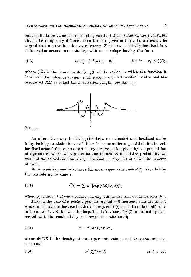
sufficiently large value of the coupling constant ~ the shape of the eigenstates should be completely different from the one given in (1.2). In part icular , he argued tha t a wave funct ion ~E of energy E gets exponential ly localized in a finite region around some site xo, with an envelope having the form

(1.3) exp [-- ~-l(E)[x -- Xo[ ] for I x - Xo[ > ~(E),

where $(E) is the characterist ic length of the region in which the funct ion is localized. For obvious reasons such states are called localized states and the associated ~(E) is called the localization length (see fig. 1.1).

q~E

Fig. 1.1.

An al ternat ive way to distinguish between extended and localized states is by looking at their t ime evolut ion: let us consider a part icle initially well localized around the origin described by a wave packet given by a superposition of eigenstates which we suppose localized; then with positive probabi l i ty we will find the part icle in a finite region around the origin after an infinite amount of t ime.

1V[ore precisely, one introduces the mean square distance r2(t) t ravel led by the part icle up to t ime t:

(i.4) r~(t) = ~ Ix]2]exp [itH] qb(x)l 2 ,

where We is the initial wave packet and exp [itH] is the t ime evolution operator. Then in the case of a perfect periodic crystal r2(t) increases with the t ime t,

while in the case of locahzed states one expects r2(t) to be bounded uniformly in t ime. As is well known, the long-time behaviour of r2(t) is in t imate ly connected with the conduct iv i ty a through the relationship

(1.5) a---- e2 D(dn/dE) /2 ,

where d n / d E is the densi ty of states per uni t volume and D is the diffusion constant :

(1.6) < r 2 ( t ) / O . . . 1 ) a s t - + ~ .

4 F. ]~fARTINELLI ~nd E. SCOPPOLA-

Using the Kubo formula , D can be expressed by

(1.7) D : l im e2 ~ }x}2<G(E q_ iv, ~'; 0, x)12>, e--~0

where G(E ~- is, v; O, x) ~- (H(v) -- E -- is)- l(O, x) denotes the Green's func-

t ion and the brackets denote the average over the configurations v of the potential .

Therefore, if only localized s ta tes are present , the conduct iv i ty a t zero

t e m p e r a t u r e should val~ish. As we will see later, the occurrence of localized states, and, therefore, the

vanishing of the conduct ivi ty , is well unders tood also f rom the ma thema t i ca l point of view in the highly disordered case ). >>1. However , one of the mos t interest ing features of the Anderson model is tha t , depending on the value of

the disorder and on the dimension of the under lying lattice, the extended and localized states can coexist. One expects the s ta tes deep in the band tails to be localized, since these are produced by deep potent ia l fluctuations, while

the states in the centre of the band are more likely to be extended a t least for a weakly disordered system. Thus, if the above pic ture is correct, a t ransi t ion in the spec t rum mus t occur f rom a localized regime to an extended one with

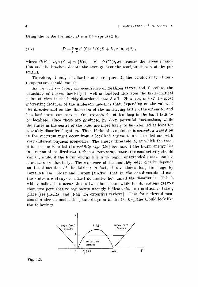
ve ry different physical propert ies. The energy threshold E c at which the t ran- sition occurs is called the mobility edge [Me] because, if the Fe rmi energy lies in a region of localized states, then at zero t e m p e r a t u r e the conduct iv i ty should vanish, while, if the Fermi energy lies in the region of extended states, one has a nonzero conduct ivi ty . The existence of the mobi l i ty edge clearly depends on the dimension of the la t t ice; in fact , i t was shown long t ime ago b y BORLA~D [Be], .~[OTT and TwosE [Mo.Tw] tha.t in the one-dimensional case the s ta tes are ahvays localized no m a t t e r how small the disorder is. This is widely believed r occur also in two dimensions, while for dimensions greater t h a n two pe r tu rba t ive a rguments s t rongly indicate t h a t a t ransi t ion is t ak ing place (see [Le.Ra] and [Nag] for extensive reviews). Thus for a three-dimensional Anderson model the phase d iagram in the (,~, E)-plane should look like

the following:

0

Fig. 1.2.

I N T R O D U C T I O N TO THE ~d[ATHEMATICAL THEORY OF ANDERSON LOCALIZATION

Hero 2Q(E) indicates the critical disorder above which only localized states exist and the two diagonal lines to the left and to the right denote the spectrum edges as functions of ~ in the case in which the potential is uniformly distributed between -- 1 and -~ 1. For an interesting discussion about the detailed shape of the diagram see [Bu.Kr.McK].

One of the most widely accepted explanation of the above picture is based on the scaling theory introduced by THOU]~ESS [Thl] and A~RAHA~S, Am- DE~SO~, LlCClARDELLO and lCA~AKRISH~A~ [Ab.An.Li.l~a]. Thouless' main idea was the following: electrons deeply loeMized inside a sample of length L should not feel a change of the boundary conditions, while extended states should be strongly affected by them. In other words, the conductivity of the sample should scale with the length L in a very different way depending on whether we are in the region of locMized states or not. In [Ab.An.Li.Ra] it was assumed that the conductance g(L) of the sample of length L i s the only relevant (dimensionless) parameter which scales according to

(1.s)

or, in a differential form,

(1.9)

g((1 ~- b ) L ) = l(g(L)),

d(in g)/d(ln L) ---- fl(g(Z)),

where fl depends only on g. For reviews on this theory see [Le.l~a], [Ab.An.Li.l~a], [An], [Is] and [Ch]. The asymptotic behaviour of the beta-function fl as g --> c~ is the classical

Ohm's law: g ( L ) ~ I f l -~ and, therefore, f l . - ~ d - - 2 . For g - + O g ( L ) , ~

exp [--Z/~] because of the exponential localization so that fl ~ in g. The values of fl(g) for finite values of g are given by perturbation theory starting from the g -> c~ limit: fl(g) .~ d - - 2 - - b/g Jr ... ~ b > O.

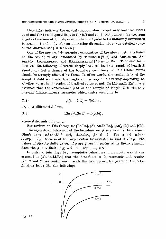
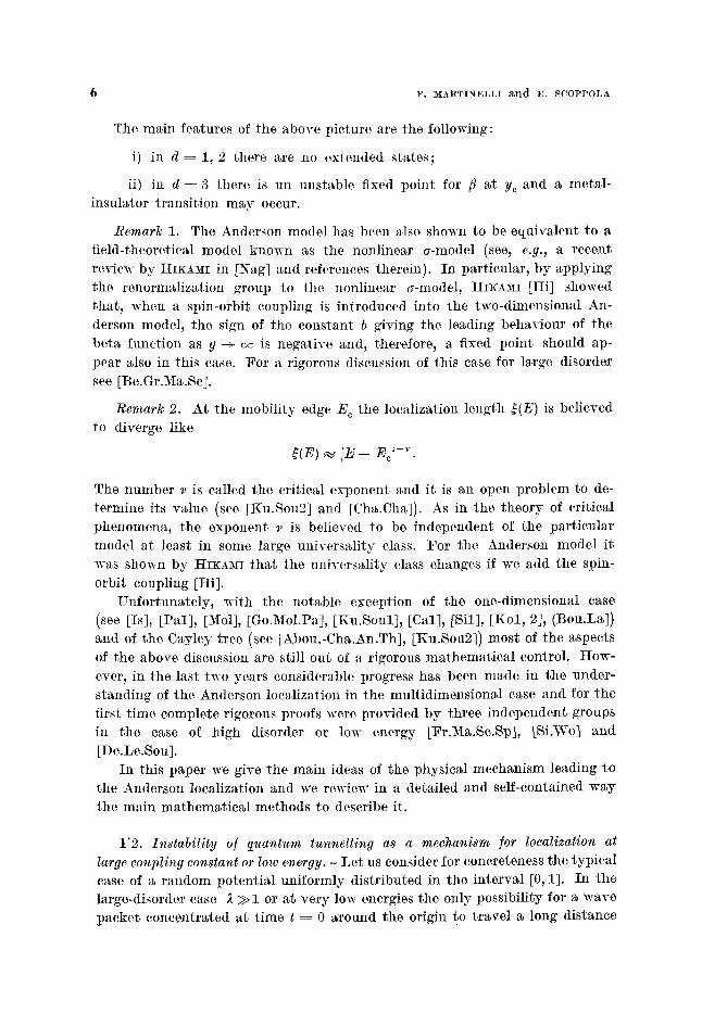
In order to join these two asymptotic behaviours in a smooth way it was assumed in [Ab.Aa.Li.Ra] that the beta-function is monoton ic and regular

(i.e. fl and fl' are continuous). With this assumption, the graph of the beta- function looks like the following:

F~. l .3 .

6 F. MARTINELLI a l l d ]g. SCOPPOLA

The main features of the above pic ture are the following:

i) in d = 1, 2 there are no extended s tates;

if) in d = 3 there is un uns table fixed point for fl a t Yc and a meta l - insulator t ransi t ion m a y occur.

Remark 1. The Anderson model has been also shown to be equivalent to a field-theoreticM model known as the nonlinear a-model (see, e.g., a recent review b y HIKA3II in [Nag] and references therein). In par t icular , by apply ing the renormMizat ion group to the nonlinear a-model, HIIr [Hi] showed tha t , when a spin-orbit coupling is in t roduced into the two-dimensionM An- derson model, the sign of the constant b giving the leading behaviour of the

be ta funct ion as g --> c~ is negat ive and, therefore, a fixed point should appear also in this case. For a rigorous discussion of this case for large disorder see [Be.Gr.ga .Sc] .

Remark 2. At the mobi l i ty edge Eo the localization length ~(E) is believed to diverge like

$(E) ~ I E - E2 -~.

The number v is called the critical exponen t and it is an open problem to de- t e rmine its value (see [Ku.Sou2] and [Ctla.Cha]). As in the theory of critical phenomena , the exponent v is believed to be independent of the par t icular model a t least in some large universa l i ty class. Fo r the Anderson model it was shown b y HrKAsiI t ha t the un iversah ty class changes if we add the spin- orbi t coupling [Hi].

Unfor tunate ly , with the notable exception of the one-dimensionM case (see [Is], [Pa l l , [Moll, [Go.Mol.Pa], [Ku.Soul] , [Call, [Sill, [Kol , 2], (Bou.La]) and of the Cayley t ree (see [Abou.-Cha.An.Th], [Ku.Sou2]) mos t of the aspects of the above discussion are still out of a rigorous ma thema t i ca l control. How- ever, in the last two years considerable progress has been made in the under- s tanding of the Anderson localization in the mul t id imensional case and for the first t ime complete rigorous proofs were provided b y three independent groups in the case of high disorder or low energy [Fr.Ma.Sc.Sp], [Si.Wo] and

[De.Le.Sou]. In this pape r we give the main ideas of the physical mechanism leading to

the Anderson localization and we rewiew in a detai led and self-contMned way

the main m a t h e m a t i c a l methods to describe it.

1"2. Instabil i ty el quantum tunnell ing as a mechanism ]or localization at

large coupling constant or low energy. - Let us consider for concreteness the typica l case of a r a n d o m potent ia l un i formly dis t r ibuted in the in terva l [0, 1]. In the large-disorder case ~ >>1 or a t ve ry low energies the only possibil i ty for a wave packe t concentra ted a t t ime t ---- 0 around the origin to t rave l a long distance

I N T R O D U C T I O N TO THE l~IATHEMATICAL T H E O R Y OF A N D E R S O N LOCALIZATION 7

is by means of quantum tunnelling through potential barriers. In fact, if the energies enter ing in the Fourier decomposition of the initial w~ve packet are smaller than Eo, with 0 < E0 << 1, or if ,~ is larg% then in most of the sites of the latt ice the random potent ia l will take values much larger than Eo because of the following simple est imate:

P(v; 0 < ~v(0) < Eo} = E0/~<< 1 .

This means tha t the regions of low potent ia l (i.e. ~v ~ Eo) which we can call the (( wells )) will have typical ly a small size and, more important~ will be separated one from the other by regions of high potent ia l which will be called (~ barriers )~. This simple observat ion makes a connection between localization and classical percolat ion [perc], bu t the main difference between them is *hat in the classical percolation problem a part icle can never overcome a potent ia l barrier, while in the quantum-mechanical case this can happen through quantum-mechanical tunnelling. Thus in this range of the parameters , the natura l question is :

why is tunnelling not e]]ective over large distances?

The key point is the following:

the delocalization o] a wave ]unction among di]]erent wells due to tunnelling is extremely unstable under perturbations o] the potential and~ therefore~ it occurs only in very special situations.

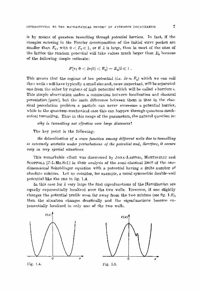
This remarkable effect was discovered by JO~A-LASI%IO~ MAI~TII~ELLI and SCOPPOLA [J-L.Ma.Scl] in their analysis of the semi-classical l imit of the one- dimensional SchrSdinger equat ion with a potent ia l having a finite number of absolute minima. Let us consider, for exampl% a usual symmetr ic double-well potent ia l like the one in fig. 1.4.

Ir~ this case for ~ very la.rge the first eigenfunetions of the t t ami l ton ian are equally exponential ly localized over the two wells. However~ if one slightly changes the potent ia l profile even far away from the two minima (see fig. 1.5)~ then the situation changes drastically and the eigenfunctions become exponential ly locMized in only one of the two wells.

v(x)!

0

V ( x ) J

x 0

Fig. 1.5. Fig. 1.4. X ~

F . M A R T I N E L L I g i l d E . S C O P P O L A

The proof of this s t r iking and unexpec ted result required the deve lopment of the new techniques, quite different f rom ~he s tandard W K B approximat ion ,

and close in spirit to the ideas of s tochast ic mechanics. The above result was extended by the same authors to potent ia ls having a

finite n u m b e r of absolute min ima by establishing a ((list of rules ~> for com- put ing the t lmnell ing [J-L.Ma.Se3]. HELFFEF, a, nd SJOSTRAND [Hc.Sj] extended it to the mul t id imensional case while Jos-.~-LAsls"IO, G~AFFI and GRECCHI [J-L. Gra.Gre] and SI)~ox [Si2] provided a proof by funct ional analyt ic methods .

In order to app ly the above ideas to the localization problem, it is, however, crucial to unders tand how does the analysis of tmmcl l ing ex tend to cases with an infinite n m n b e r of wells. This is in genera.1 a ve ry difficult p rob lem and it is impor t an t to provide models which arc simple enough to be analysed in full detai l bu t also sufficiently typica l to give a clue as to what happens in the

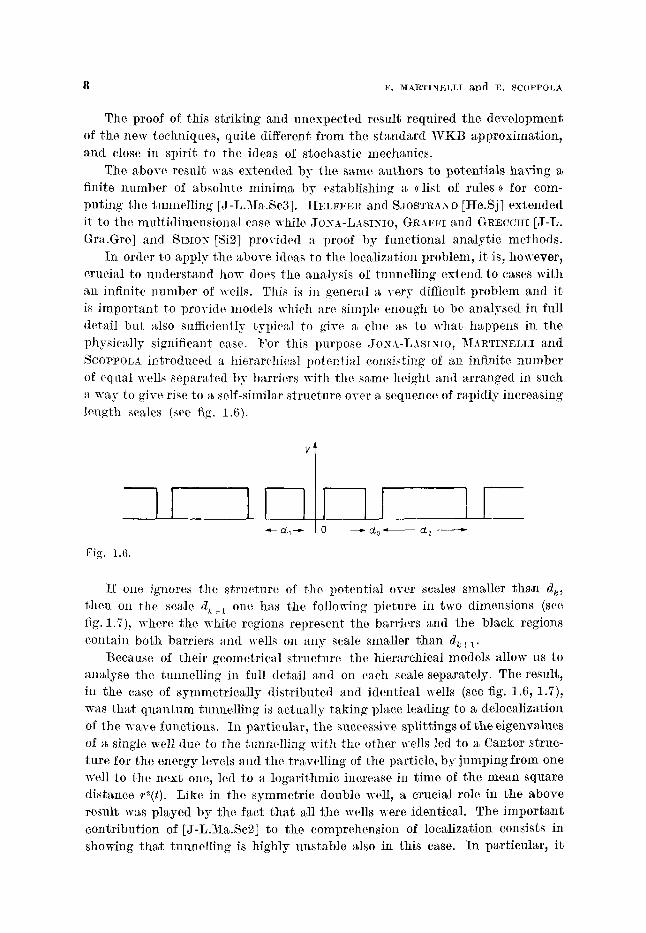
physical ly significant case. For this purpose Jo~t-L.xsIS'm, ~[ARTINELLI and SCOPPOLA in t roduced a hierarchical potent ia l consisting of an infinite n u m b e r of equal wells separa ted by barriers with the same height and ar ranged in such a way to give rise to a self-similar s t ruc ture over a sequence of rapidly increasing length scales (see fig. 1.6).

V l c/. 1 0 - - ~ Cs 0 cL z . - ~

Fig. 1.6.

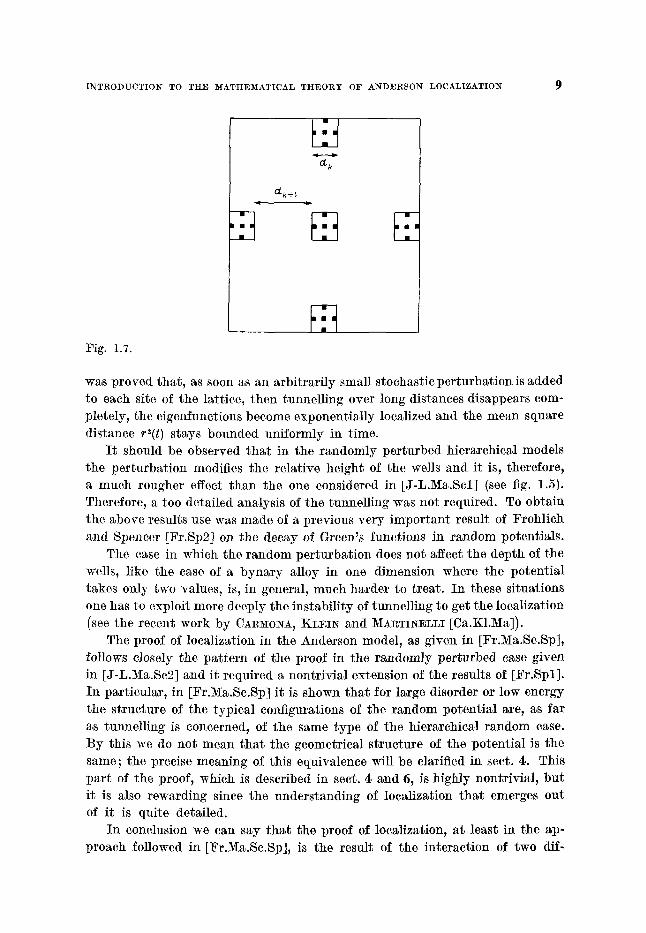
I f one ignores the s t ruc ture of the potenti~d over scales smaller t han dk, then on the scale dk~ 1 one has the following pic ture in two dimensions (see fig. 1.7), where the white regions represent the b~rriers and the black regions

contain bo th barr iers and wells on any scale smaller t han d~+ t. Because of their geometr ical s t ruc ture the hierarchical models allow us to

analyse the tmmel l ing in full det~il and on each scale separately. The result, in the ease of symmet r ica l ly dis t r ibuted and identical wells (see fig. 1.6, 1.7), was t ha t q u a n t u m tunnell ing is actual ly tak ing place leading to a deloealization of the wave functions. In par t icular , the successive split t ings of the eigenvMues of a single well due to the tunnell ing with the other wells led to a Ca.n~or structure for the energy levels and the t ravel l ing of the particle, by jumping f rom one well to the nex t one, led to a logari thmic increase in t ime of the mean square dis tance r~(t). Like in the symmet r ic double well, a crucial role in the above result was p layed b y the fac t tha~ all the wells were identieM. The i m p o r t a n t cont r ibut ion of [J-L.Ma.Sc2] to the comprehension of localization consists in showing tha t tunnel l ing is highly uns table also in this ease. In par t icular , i t

I N T R O D U C T I O N TO T H E I~IATHEMATICAL T H E O R Y OF A N D E R S O N L O C A L I Z A T I O N

~ r / k F

Ctk+~

Fig. 1.7.

was proved that, as soon as an arbitrarily small stochastic perturbation is added to each site of the lattice, then tunnelling over long distances disappears completely; the eigenfunctions become exponentially localized and the mean square distance r2(t) stays bounded uniformly in time.

I t should be observed that in the randomly perturbed hierarchical models the perturbation modifies the relative height of the wells and it is, therefore, a much rougher effect than the one considered in [J-L.Ma.Scl] (see fig. 1.5). Therefore, a too detailed analysis of the tunnelling was not required. To obtain the above results use was made of a previous very important result of Frohlich and Spencer [Fr.Sp2] on the decay of Green's functions in random potentials.

The case in which the random perturbation does not affect the depth of the wells, like the case of a bynary alloy in one dimension where the potential takes only two values, is, in general, much harder to treat. In these situations one has to exploit more deeply the instability of tunnelling to get the localization (see the recent work by CA~ONA~ KLEI~ and 1V~AI~TINELLI [Ca.K1.Ma]).

The proof of localization in the Anderson model, as given in [Fr.Ma.Sc.Sp], follows closely the pattern of the proof in the randomly perturbed case given in [J-L.~a.Sc2] and it required a nontrivial extension of the results of [Fr.Spl]. In particular, in [Fr.Ma.Sc.Sp] it is shown that for large disorder or low energy the structure of the typical configurations of the random potential are, as far as tunnelling is concerned~ of the same type of the hierarchical random case. By this we do not mean that the geometrical structure of the potential is the same; the precise meaning of this equivalence will be clarified in sect. 4. This part of the proof, which is described in sect. 4 and 6, is highly nontrivi~], but it is also rewarding since the understanding of localization that emerges out of it is quite detailed.

In conclusion we can say that the proof of localization~ at least in the approach followed in [Fr.~a.Sc.Sp], is the result of the interaction of two dif-

1 0 F. MARTINJgLLI and E. SCOPPOLA

ferent kinds of ideas. On the one hand, one has the instabi l i ty of tunnell ing which provides a key for the unders tanding of the physical mechanism of localization and, therefore, su~ ' c s t s the ri~'ht questions to ask. On the other hand, one has the analysis of the Green's funct ion and the organizat ion of the probabi l is t ic es t imates of [Fr .Spl] main ly based on ideas developed for the s tudy of the

Koster l i tz and Thouless t ransi t ion in the two-dimensional Coulomb gas [Fr.Sp3]. The frui tful interact ion between these different id(,as consisted in re in terpre t ing the scheme of [Fr .Spl] as an implicit analysis of tunnell ing and in extending their techniques to prove the instabi l i ty of tm~uelling in complicated eases

like the Anderson model. The hierarchical model has been the meet ing point of these two approaches. In this connection w~ should ment ion tha t Jo~xa- L i s i x i o cont r ibuted in a de te rminan t wa.y to tire fo rmat ion of the point of view presented in this paper. In par t icular , he pointed out the similari ty between the tunnel l ing effects in the hierarchical case and in the Anderson model . This observat ion suggested t ha t the typica l configurations of the r andom potent ia l in the Anderson model have the same s t ructure of those in the

hierarchical case.

1"3. L o c a l i z a t i o n at i ~ t e r m e d i a t e d i s o r d e r . - The above discussion applies t.o a.ll cases in which the localization length ~(E) (see (1.3) and sect. 4 for a more precise definition) is of order of the latti( 'e sl)acing , namely ~(E) ~ 1. Howe~-er, as a l ready explained before, there are in te rmedia te regimes in the disorder energy plane in which the localization length is still finite but large compared with the lat t ice spacing. In order to prove localization in these cases, a possible strateo'y is the following:

i) One first shows t h a t with large prob~bi l i ty the eigenstates with energy E axe exponent ia l ly loea.lized only on clusters of sites of Z d of size l

at a typ ica l distance l' >>/ one f rom the other.

ii) Using the same idea.s and techniques valid in the high-disorder case, one then proves t ha t each eigenstate is actual ly localized on a small n u m b e r of the above clusters and it decays exponent ia l ly outside them. Like in stat is- t ical mechanics, the reason is t h a t on any scale larger t han 1 the sys tem will (( look like )) a weakly coupled sys tem (or a highly disordered one) which can be t rea ted in pe r tu rba t ion theory. The localization on the scale l will, therefore, p ropaga te to all successive scales giving rise to the exponent ia l decay of the eigenfunctions.

The first step requires to control a complicate mechanism of des t ruct ive interference which in one dimension has been anMysed by means of the t ransfer ma t r i x formalism. This teclmique, however, has no counterpar t in the mult i - dimensional ease and, therefore, a complete proof of localization a t in te rmedia te

disorder is still missing.

INTRODUCTION TO THE M A T H E M A T I C A L T H E O R Y OF ANDERSON LOCALIZATION l l

The second step is p a r t of this work and it is described in details in sect. 4-6 and appendix B.

The p a t t e r n of the proof goes as follows: we will p rove localization under

two main assumpt ions which are described below and then we will show in which cases these assumpt ions are verified (e.g., large disorder or low energy).

In ma thema t i ca l t e rms in order to p rove localization in a neighbourhood of a given energy E in the spec t rum of the t t ami l ton ian H we will need to assume the following:

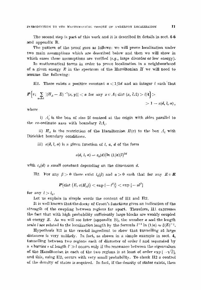
t t l . There exists a posi t ive cons tan t a < 1/2d and an integer l s u c h ' t h a t

e{v; ~, I(HA-- E)-~(x, Y)I < a for any x ~ A ; dis t (x, ~A)> 1/4}> v~SA

> 1 -- ~(d, l, a ) ,

where

i) A] is the box of size 21 centred at the origin wi th sides paral lel to the co-ordinate axes wi th bounda ry ~Jl z.

ii) H A is the restr ic t ion of the ~ a m i l t o n i a n H(v) to the box A l wi th Dirichlet boundary conditions.

iii) e(d, l, a) is a given funct ion of l, a, d of the fo rm

e(d, l, a) = eo(d)(ln (lla)ll) 2a

with so(d ) a small cons tant depending on the dimension d.

H2. For any fi > 0 there exist lo(fl) and ~ > 0 such t h a t for any E e R

P{dist (E, a(HA) ) < exp [--/~]} < exp [ - - ~l ~]

for any l > l o.

Le t us explain in simple words the content of H1 and H2. I t is well known t h a t the decay of Green's functions gives an indicat ion of the

s t rength of the coupling between regions far apar t . Therefore, I t l expresses the fact t h a t with high probabi l i ty sufficiently large blocks are weakly coupled a t energy E. As we will see la ter (appendix B), the number a and the length scale 1 are re la ted to the localization length by the formula 1-1 In (l /a) ~ ~(E) -1.

Hypothes is H2 is the crucial ingredient to show tha t tunnell ing a t large distances is ve ry unlikely. I n fact , as shown in a simple example in sect. 4, tunnel l ing between two regions each of d iameter of order l and separa ted b y a <( barr ier ~> of length l' >> 1 occurs only if the resonance between the eigenvalues of the Hami l ton ian in each of the two regions is at least of order exp [--V/Y], and this, using H2, occurs with ve ry small probabi l i ty . To check H2 a control of the densi ty of s tates is required. In fact , if the densi ty of s tates exists, then

1 2 F. MARTINELLI a n d E. SCOPPOLA

the typica l spacing between the (2l) 4 eigenvalues of H A is of order 1/(21)~>> >>exp [ - - I z] and we expect H2 to hold. In mos t cases (see corollary 3.1) we will ver i fy I t2 by mak ing a suitable cont inui ty assumpt ion on the single-site po ten t ia l dish~ibution. In the one-dimensional case, however, t t2 holds for any potent ia l dis t r ibut ion provided i t has some finite moment .

1"4. Description o] the main results. - We now turn to the descript ion of the

main results of this paper . Le t us assume tha t for a ~'iven energy E the Hami l ton ian H(v) satisfies H I

and tI2. Then:

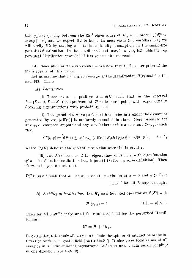
A) .Localization.

i) There exists a posi t ive 6--- -6(E) such t ha t in the in terva l I - - [ E - - 6 , E ~-6] the spec t rum of H(v) is pure point with exponent ia l ly

dec,~ying eigenfunctions with probabi l i ty one.

ii) The spread of a wave packe t with energies in I under the dynamics genera ted by exp [itH(v)] is mfiformly bounded in t ime. More precisely for any % of compac t suppor t and any ~ > 0 there exists tt cons tant C(n, %) such

tha t

Ix l"[exp [itH(v)] P~(H)~0(x)l" < C(n, % ) , t > 0,

where PI(H) denotes the spectral project ion over the in terval I .

iii) Le t E'(v) be one of the eigenvalues of H in I with eigenfunetion

~v' and let ~' be its localization lenlsth (see (4.18) for a precise definition). Then

there exist p > 0 such t h a t

P{gE'(v) c I such t ha t ~ ' has a.n absolute m a x i m u m at x --~ 0 and ~' > / 5 } <

< L -p for all L large enough .

B) Stability o] localization. Let H 1 be a bounded opera tor on 12(Z d) with

Hl(X , y) = 0 if [ x - y f > 1.

Then for ~11 6 sufficiently small tile results A) hold for the pe r tu rbed I-Iamil-

tonian :

H ~ = H + 6H I .

In part icular , this result allows us to include the spin-orbit in teract ion or the in- te rac t ion with a magnet ic field [Be.Gr.Ma.Sc]. I t also gives localization a t all energies in a bidimensional anysot ropic Anderson model with small coupling

in one direction (see sect. 9).

I NTRO D U CTI O N TO THE I~ATt tEMATICAL T I t E O R Y OF ANDIilRSOlq LOCALIZATION 13

We now tu rn to discuss under which conditions on the pa rame te r s A and E and on the po ten t ia l dis tr ibution dP(v) hypotheses I t1 and 112 hold.

C) Validity o] 111 and 112.

i) I f d = i and if fdP(v)]v[~< q- ~ for some fi > 0~ then 111 and 112 hold for a n y ~ > 0 and any E e R.

ii) I f d > 1 and if the dis tr ibut ion funct ion of dP(v) is I to lder con-

t inuous, then 112 holds for any X > 0. Fur the rmore , there exists a Xr > 0 such t ha t for a n y X > ~ 111 holds for any energy E and~ if A < Ao, then 111 holds

for all energies E close enough to the spec t rum edges.

iii) Suppose t h a t the dis tr ibut ion funct ion dP(v) is 1[older cont inuous and assume t h a t in the energy in te rva l I the following es t imate holds:

r(n)( t, ~o, I ) < eonst .t for any t > O .

Then, if n is large enough~ 111 holds for any energy E ~ I .

This interest ing resul t t ha t appears here for the first t ime shows t h a t condition 111 is close to be op t imal in order to get localization. I n particular~ it suggests t h a t localization other t h a n exponent ia l is absent and t h a t the energy threshold a t which the localization length diverges mus t coincide with the energy where the conduct iv i ty becomes posit ive.

We conclude with a discussion on the extension of our results to the continuous Schr6dinger equat ion with a r andom potent ial . The model t h a t we will discuss in sect. 10 describes the mot ion of an electron in a sea of randomly d is t r ibuted impuri t ies which generate an a t t r ac t ive poten t ia l whose s t rengths depends on the impur i t y in a r andom way. More precisely we have

(1.10) H = - - A + ~ q~ Vo(x - - x~),

where {x~} is a Poisson process on R d with densi ty @, the qi's are i.i.d, r a n d o m

variables uni formly dis t r ibuted in [0, 1] and V 0 is a nonposi t ive bounded func- t ion with suppor t in the uni t sphere.

D) Localization in the continuous case. For @<< 1 the negat ive p a r t of the spec t rum of H consists of a dense set of eigenvalues with exponent ia l ly decaying eigenfunctions.

The proof of these results can be found according to the following scheme:

A) is p roved in sect. 4-6 for large coupling cons tant ~. In the more general case when only H1, 112 hold, i t is discussed in appendix ]3;

B) is p roved in sect. 9;

14 F. MARTINELLI and 1~. SCOPPOLA

C) i) is d i scussed in sect . 7 whi le C ii), iii) a r e d i scussed in sect . 3,

4 a n d 8, r e s p e c t i v e l y ;

D) is t h e s u b j e c t of sect . 10.

1"5. Localizatio~t in other phys ica l systems. - W e br ief ly desc r ibe now some

o t h e r d i s o r d e r e d s y s t e m s to which our t e c h n i q u e s can be ~ppl ied .

1) H a r m o n i c vibrations of a crystal lattice. L e t us cons ide r an in f in i te

a r r a y of coup l ed h a r m o n i c osc i l l a to r s each one a t tn .ched to a s i te of t h e l a t -

l i c e Z a. T h e cqua. t ion of m o t i o n s of t h e osc i l l a to r s a re

(1.1.1) x_j = -- (, ,~xj-~ 2 ~, K~,i(x ~, -- x j ) , xj e R '~, j"

where , for e x a m p l e , K ; j = 0 unless I J ' - - J [ = 1.

The v a r i a b l e s (,)j :rod K~,j m a y be a s s u m e d to be i . i .d, r a n d o m v a r i a b l e s

d i s t r i b u t e d in some b o u n d e d i n t e r v a l of [0, - - o.) . The m o d e l speci f ied b y

(1.11) descr ibes t h e h a r m o n i c v i b r a t i o n s of a d i s o r d e r e d l a t t i c e . 111 o r d e r to

so lve eqs. (1.11), one e x p a n d s t h e so lu t ions in t e r m s of t h e ~wrmal modes

def ined as t h e e igen func t ions of t h e J a c o b i m a t r i x .(2'-' g iven b y

(1.1._,) . % =

) .K;j , if '.i - - Jl - : I ,

- - ( - - '"~ @ ~:,s ~ l ; ' N ; ~ ) ' if i = j , 0 . o t h e r w i s e .

This is a <~ t i~ 'ht b i n d i n g ~> H a . m i l t o n i a n w i t h diago;~al d i so rde r

(1.13)

a n d oJ]-diagonal d i s o r d e r

(1.14)

' J:l~-;I 1

{XK;~}.

I f , for e x a m p l e , ogj ~ 0 for ~Q1 j ' s a n d if 2 is l~rgc enough , o11e m a y ~ p p l y t h e

t e chn iques d e s c r i b e d ill th i s w o r k to show t h a t t h e n o r m a l m o d e s of ~ {x~ ~

yy} (y~ = d/dtx~) w i th f r e q u e n c y o ) > 0 a re e x p o n e l ; t i a l l y loca l i zed in t h e p h a s e C a = 0 space . The re is, however , a h v a y s an e x t e n d e d s t a t e ~ cons t c o r r e s p o n d i n g

to t h e gene ra l i zed ei~ 'envalue eo - - 0 a n d one exl)ects t h e loeMiza t ion l e n g t h

~(~o) to d ive rge qs co -~ 0. I n t h c o n e - d i m e n s i o m ' l case th i s r e su l t s has been

est ,~blished in [De .Ku .Sou] .

2) Wavegu ides wi th r a n d o m boundaries . L e t us cons ide r t h e s imple

wa.ve e q u a t i o n in ~n u u b o u u d e d d o m a i u S of R ~, d = 2, 3, e.g. ~t~ in f in i t e s lab

INTRODUCTION TO THE ~ATHEMATICAL THEORY OF ANDERSON LOCALIZATION 1 5

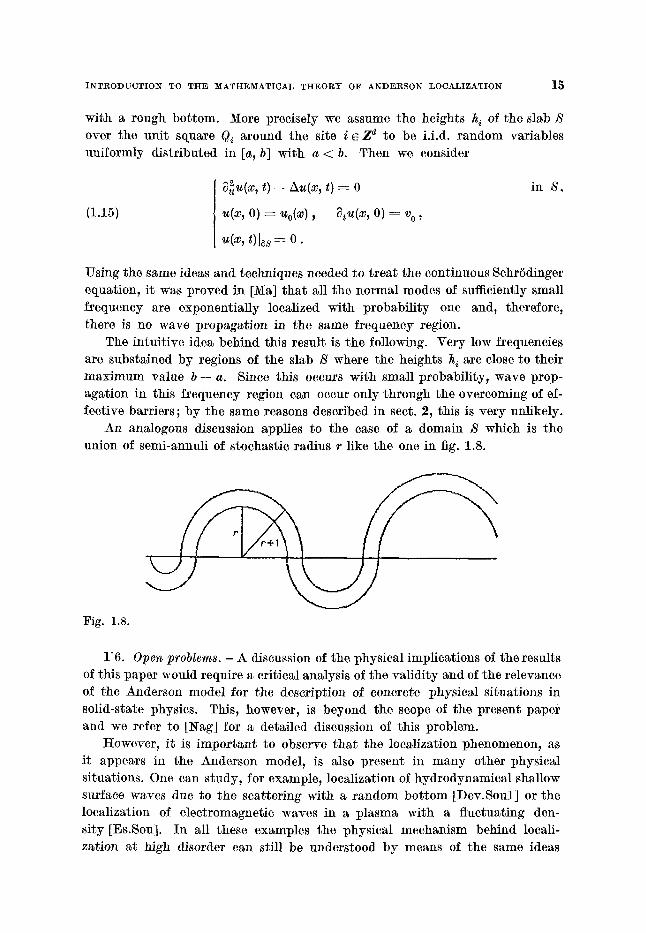
with a rough bot tom. More precisely we assume the heights h~ of the slab S over the uni t square Q~ around the site i e Z d to be i.i.d, random variables uniformly dis t r ibuted in [a, b] with a < b. Then we consider

(1.15)

~ u ( x , t) - A u ( x , t) = 0

u ( x , O) = Uo(X) , ~ t u ( x , O) = v o ,

u ( x , t ) les = O.

in S,

Using the same ideas and techniques needed to t r ea t the continuous Schr6dinger equation, it was proved in [Ma] tha t all the normal modes of sufficiently small f requency are exponential ly localized with probabi l i ty one and, therefore~ there is no wave propagat ion in the same f requency region.

The intui t ive idea behind this result is the following. Very low frequencies are substained by regions of the slab S where the heights h~ are close to their max imum value b - a. Since this occurs with small probabil i ty, wave prop- agation in this f requency region can occur only through the overcoming of effect ive barriers; by the same reasons described in sect. 2, this is very unlikely.

An analogous discussion applies to the case of a domain S which is the union of semi-annuli of stochastic radius r like the one in fig. 1.8.

:Fig. 1.8.

1"6. Open problems. - A discussion of the physical implications of the results of this paper would require a critical analysis of the val idi ty and of the relevance of the Anderson model for the description of concrete physical si tuations in solid-state physics. This, however, is beyond the scope of the present paper and we refer to [Nag] for a detailed discussion of this problem.

However, it is impor tan t to observe tha t the localization phenomenon, as it appears in the Anderson model, is also present in m an y other physical situations. One can study, for example, localization of hydrodynamica l shallow surface waves due to the scat ter ing with a random bo t tom [Dev.Soul] or the localization of electromagnetic waves in a plasma with a f luctuat ing densi ty [Es.Sou]. In all these examples the physical mechanism behind loca l - zation at high disorder can still be understood by means of the same ideas

16 F. )IARTINELLI and E. $COFPOLA

discussed '~bove for the Anderson model and the same scheme of proof can be easily adap ted at least in all the cases in which the sys tem can be described by means of a r a n d o m linear differential equat ion of the wave type . I t is an i m p o r t a n t and open problem to s tudy the effects on the localization of the nonlinear corrections. For recent results in this direction see [Dev.Sou2]

and [Fr.Sp.~Va]. We believe, however, t ha t a be t te r unders tanding of the role of localization

in physical sys tems requires a much more complete ma thema t i ca l comprehension of the problem. In par t icular , several interest ing aspects of localization

are still open f rom the ma thema t i ca l point of view. We ment ion, for example ,

i) localization for a rb i t rar i ly weak disorder in two-dimensional sys tems;

ii) existence and na ture of the Anderson t ransi t ion in three dimensions; this ve ry difficult p rob lem includes in te rmedia te and p robab ly easier questions

like the (possible) existence of polynomi~l ly localized s ta tes or the absence under very general conditions of the singular continuous spec t rum;

iii) r andom potent ia ls with correlations between separa ted sites. Par - t icular ly interest ing cases are the a lmost periodic potent ia ls wi th more t h a n one frequency, e.g.

V(~) = ).(COS (0)1 n ~- Xl) -[- COS (o)2n -~ X2) ) , n ~ Z .

For recent results in the case of one f requency see [Sin].

2. - Definitions and mathematical background.

For the reader ' s convenience in this section we collect definitions, assumptions and s tandard results used in the paper .

S p e c t r a l a n a l y s i s . Let H be the H a m i l t o n i a n o n 12(Zd):

(2.1) /Uv) = - A + ~v,

where - - A is the finite-difference Laplac ian given b y

(2.2) - - A ( x , y) =

and ~ > 0 is a coupling constant .

2 d , if x = y ,

- - :1 , if ]x--y[=l,

0 , o therwise ,

The r a n d o m potent ia l v is a collection of r andom variables v ( x ) , x E Z ~,

independent , identical ly d is t r ibuted (i.i.d.), with common distr ibution dP(v);

I N T R O D U C T I O N TO THE M A T H E M A T I C A L T H E O R Y OF A N D E R S O N L O C A L I Z A T I O N 1 7

therefore, a potential configuration is a point in the probability space ~ - ~ z ~ ( R , dP(v(x))). On the probabihty distribution dP(v) we make the

following general assumptions:

A1) Holder continuity. There exist a oc ~ (0, 1] and a constant C such that for each a, b e R , 0 < b - - a < 1 ,

(2.3) b

f dP(v) < C ( b - a) ~ . a

A2) Existence o/ a /inite moment.

f]vl~dP(v) < co for some k < o o .

In some cases, like the one-dimensional Anderson model, we will be able to relax considerably assumption A1 by including, for example, the Bernoulli measure dP(v) ---- p~(v = O) -4- (1 -- p) ~(v = 1).

By abuse of notations we will denote by P the product measure

d P = [ I dP(V(x) ) xeZ a

and by E{.} the expectation with respect to it. We denote by a(H) the spectrum of the self-adjoint operator H. I t is well

known (see, e.g., [Re.Si]) that the spectrum can be decomposed into its pure point, absolutely continuous and singular continuous components:

r = G (H) u v

where -- is the closure simbol. This decomposition is obtained as follows:

if dpv is the spectral measure associated with the vector Yh that is, if

s ]()t)d~v for each ] e Co(R), where ( . , . ) denotes the scalar (v,/(H) V) )

product in l~(Zd), from the decomposition of the measure d~v in pure point, absolutely continuous and singular continuous component we obtain the following decomposition of the Hilbert space ~----- l~(Zd):

~,D= {~0[r is pure point}, 5(far ~ {%o1r v is absolutely continuous with respect to Lebesgue measure},

~%fs~=r {YJ[r is continuous singular with respect to Lebesgue measure}.

Iqow we have [Re.Si]:

18 r. ~IARTINELLI and E. SCOPPOLA

The restr ict ion of H to ~ : H ~ , , has a complete set of eigenfunctions

and %p(H) = (E[E is an eigenvalue of H}. The restr ict ion of H to ~ ~ o has only absolute ly continuous spectral measures and ~ r analogously H ~ has only continuous singular spectral measures and

Finally~

~,us(H) = {E]E is an eigenvMue of finite mult ipl ic i ty and an isolated point of ~(~)}.

We conclude this pa r t by discussing an eigenfunction expansion of H which will link the propert ies of its eigenfunetions with t ha t of t ime-dependent quantit ies like r2(t).

A funct ion ~0 on Z ~ is called a get~eralized eigenJunction of the t t ami l ton ian H(v), corresponding to a generalized eigenvalue E(v) if and only if y~ is a polynomial ly bounded solution to the equat ion

( H ( v ) - - E ) ~ = O .

We have the following basic result [Ber], [Si3]:

Theorem. i) For a lmost every energy E with respect to the spectral measure ~o(v) of H(v), there exist solutions of the equat ion

which satisfy

(B(v) - E) ~ = 0

Iw~(x)l < c ( 1 + lx12) d/2+'

for any ~] > 0 and some posi t ive constant C.

ii) For any g r C(R) and x, y ~ Z a

g(H)(x, y) = f d o ( E ) g(E) yJE(x) yJ~(Y) .

Remark. We are using here the fact t h a t with probabi l i ty one the spec t rum of H is simple (see [De.Le.Sou].)

Although the above result looks ra ther abs t rac t since very li t t le is known abou t the spectral measure d@, the generalized eigenfunctions will p lay a crucial role in the fu ture discussion (see also [Pa.1]).

Ergodic properties. We recall now some general ergodic property useful in the de terminat ion of the spec t rum (see sect. 3).

Le t {T~}~z~ be the shift t r ans format ion

( T~ v)(y) = v(y -~ x) .

I N T R O D U C T I O N TO T H E M A T H E M A T I C A L T H E O R Y OF A N D E R S O N L O C A L I Z A T I O N 19

Since the r a n d o m variables v are i.i.d., the shift t ransformat ions are ergodic in the sense tha t , if an event A c s is invar ian t under the shift t r ans format ion

T ~ I A - = A, then its p robabi l i ty P(A) is zero or one. By the ergodic theorem

we have: if / is a measurab le funct ion on ~2, shi f t - invar iant /(v) = / (T~v) , then there is a subset of ~2 of measure one in which / is constant .

Le t now U~ be the un i t a ry opera tor on/2(Zd) given b y (U~)(y) = ~v(y -4- x);

we have immedia t e ly

uflI(v) U [ l = tt(T~v) .

Boundary conditions. I n our discussion of localization we will often need

to consider the restr ict ion of the Hami l ton ian H to finite subsets of the lat t ice Z d wi th Dirichlet or 2Veumann boundary conditions. I n the discrete case this

can be done as follows: let A be a subset of Za~ and let

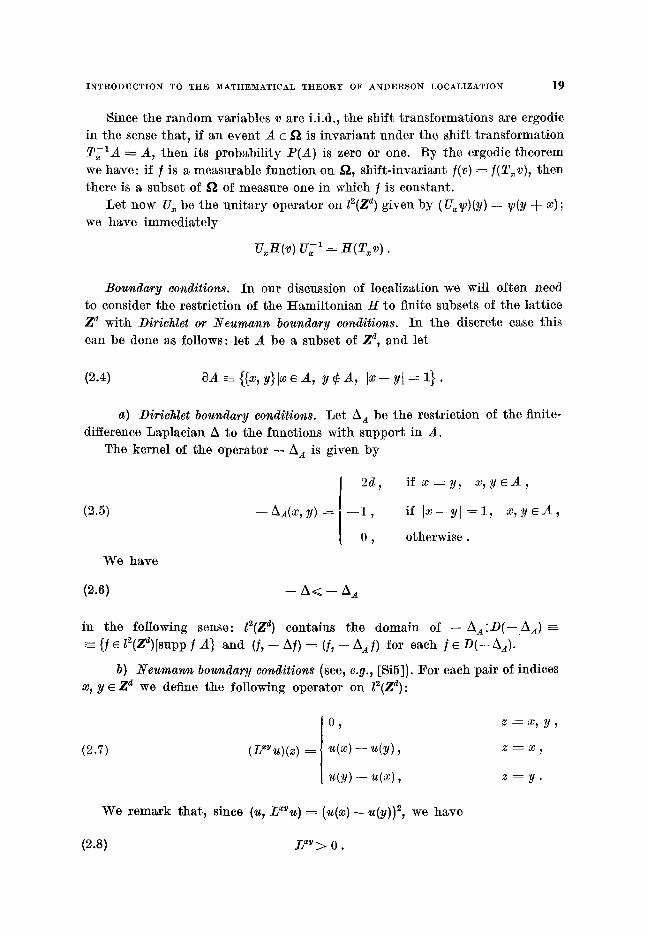
(2.4) 8A~((x,y)lx~A , y~A, lx - -y t= l } .

a) Dirichlet boundary conditions. Let A A be the restr ic t ion of the finite- difference Laplac ian A to the funct ions with suppor t in A.

The kernel of the opera tor - - A a is given b y

(2.5) - - h a ( x , y) =

We have

2d~ if x = y , x, y E A ~

- - 1 , if ] x - - y ] - ~ l , x, y e A ,

0 ~ o therwise .

(2.6) - - A ~ - - A a

in the following sense: le(Z a) contains the domain of - - A ~ : D ( - - A a ) ~- {] e/2(Zd)[supp ] A} and (], - - A]) = (], - - A a ]) for each ] e D ( - - An).

b) s boundary conditions (see, e.g., [Si5]). Fo r each pair of indices x~ y e Z d we define the following opera tor on /2(Zd):

(2.7) (LXVu)(z) =

O~ Z~--x~ y~

u(x) - -u (y ) , z = x ,

u ( y ) - - u ( x ) , z = y .

We r e m a r k tha t , since (u, Z~' u) = (u(x) -- u(y)) 2, we have

(2.8) J5 ~v > 0 .

2 0 1% MARTINELLI and ]~. SCOPPOLA

Moreover,

(2.9) A _ ~: L ~ ,

where each pair in the sum is counted once. The Neuma rm finite-difference Laplac ian is now defined as follows:

(2.1o) - A~ = - - A - - 5 L ~ ; (z,v)~OA

(2.6) and (2.6) imp ly the Di r ich le t -Neumann bracket ing:

(2.11)

Green's /unctions. A major role in the s tudy of localization is p layed by the Green's funct ion of the Hami l ton ian H. Fo r a fixed v ~ f~ and E, we define

(2.12) G(E + is, v; x, y) ~ (H -- E -- i s ) - l (x , y) .

I f A is a subset of Z d, let H d(v ) be the restr ict ion of the opera tor H to A

with Diriehlet bounda ry conditions HA(v ) ~ -- A A + JtvY~, where ~V A is the characteris t ic funct ion of the set A, and G~(E + is, v; x, y) the corresponding Green 's f lmction. This ma t r ix is defined only for x and y in A, but we can ex tend it to the full la t t ice by set t ing G d(E + is, v; x, y) = 0 unless x and y belong r A.

As we will see in sect. 5, one of the basic tools in the s tudy of the decay propert ies of the Green's funct ion following the s t ra tegy of Frohlieh and Spencer consists in adding ex t ra Diriehlet boundary conditions inside a given set B and to r emove t h e m in pe r tu rba t ion theory. In order to do tha t , we need formula which relates the Green's funct ion with the addi t ional bounda ry con-

ditions to G~. Le t B be a subset of A, then the I t i lbe r t space associated with

A:12(A) can be wr i t ten as a direct sum

12(A ) = 12(B) @ le(A~B)

and the Hami l ton ian H A is g iven b y

/7 A = H . §

where the opera tor F corresponding to the coupling be tween B and A \ B is given b y

1, if (x,y)�9 (2.13) F(x, y) = 0 , o therwise .


Clearly G~, x ~ G~ ~ - G A \ ~ is the Green's function of the t Iamil tonian H~ ~- //AN r . By the Jirst resolvent identity we have

(2.14) G ~ -= G B, A + G ~,x FG A = G B,~ -~ d ~ FG B, ~ .

We recall now an additional result on the decay of the Green's function known as the Combes-Thomas argument. Let z e C be such tha t dist (z, a(HA) ) = (3, then

(2.15) IG(z, v; x, y)l < 2(3-1 exp [ - m((3)lx- yl]

wi th m ( 3 ) = in ((3(4d)-1-{-1) and the distance between two sets A and B defined by dist (A, B) ~ inf [a -- b] with I" I the Euclidean distance.

a e A , b e B

In order to verify (2.15), we consider the multiplication operator on 12(Z e) given by U(a)(p, q) ~ e x p [iap](3v~ , p, q ~ Z ~. We have

U(-- a)H~(v) U(a) -= HA(v) -~ Q(a)

wi th Q(a), bounded operator independent of v, satisfying

Q(a) < (e~p [lal] - 1) 2d for a ~ C a.

For [a[ < in (3(~d) -1 -[- 1) we have Q(a) < (3[2 and thus

U(-- a) fin(z) U(a) = [H a - z q- Q(a)] -1 ( 2/(3.

This implies

I[U(-a)GA(z) U(a)](x, Y)I = [exp [is. ( y - x)] Gx(z , v; x, y)[ < 2/(3.

By going to imaginary a with {a] = I n ( ( 3 ( 4 d ) - 1 - ~ - 1) We obtain (2.15). ~or small 3 we can pu t m(3) = (3/4d.

We conclude this short list of mathematical tools with a well-known probabilistic result tha t will be used several times.

.Semma (Borel-Cantelli). Let ~ be a probabili ty space with measure P and let -~k c ~ be a sequence of events. I f ~ P ( F k) < c~, then the probabili ty

k

t h a t / ~ be verified an infinite number of times is zero, tha t is

co

-(n u n = l k > n +

~o

<lir% ~ P ( F k ) ~ 0 by hypothesis. k ~ n

~ - - l i m e ( U Fk)

22 F. MARTINELLI and E. SCOI'POLA

3. - Ergodic properties of the spectrum and the density of states.

In this section we will give some general results on the Hami l ton iun of the Anderson t ight -binding model defined in sect. 1 and 2.

We first discuss the a lmost surely nonstochast ic character of the spec t rum which represents the beginning of the rigorous t r a t e m e n t of the Anderson model.

Subsequent ly we will discuss regular i ty propert ies of the densi ty of s tates and its behaviour near the edges of the spectrum. As we will see later, these results are i m p o r t a n t in our s tudy of localization. The ergodic propert ies of the spectrum, (see e.g., [Pa2], [Ku.Soul] , [Ki.Ma.1]) are actual ly l~rgely model

independent and are due to the ergodic charac ter of the r andom field modell ing the potent ial . We will discuss t hem only in the context of the Anderson model and we refer the ma thema t i ca l ly inclined reader to [Ki .Mal] for a more general discussion iI1 the f r amework of a rb i t r a ry ergodie self-adjoint r andom operators on a separable Hi lber t space.

The main theorem reads as follows:

Theorem 3.1. There exists a set ~o c ~ of P -measu re one and subsets of R, 2:, Zpp, 2:ac such t h a t for any v ~ ~ o we have

~) ~(H(~)) = r , ~oo(R(~)) = Zoo, ~o(E(~)) = Z,o;

b) adi~(H(v)) = O.

See append ix A for the proof.

The nex t result is an explicit description of the set 27 which is due to K v ~ z and SOUILLARD [Ku.Soul] .

Le t for any set A and B in R be A + B = {~ E R ; there exist 2~ e A and 22 e B such t h a t 2 = ~1 + ~.~} and let Z o be the topological suppor t of the p robab i l i ty men, sure P(dv), t h a t is t he set of all possible values of the poten t ia l v. Then we have

Theorem 3.2.

= [o, 4d] + ~Zo,

where 27 is the a lmost surely constant spec t rum of H(v).

Sketch o] the proo]. Since []--AIj = 4d, it follows immedia te ly t h a t dist (ZT, ~ o ) < 4d, so t h a t 27 c 2Z o + [0, 4d].

We have to show the converse:

(3.1) [o, 4a] + 2Zo c z .

The basic idea behind all this k ind of results is the following: since the potent ia l is a collection of i.i.d, r a n d o m variables, t hen for any Vo~ Zo, any

INTRODUCTION TO THE MATHEMATICAL THEORY OF ANDERSON LOCALIZATION 2 ~

s > 0 and any Z c N it is possible to find, with probabi l i ty one, x 0 e Z a such that

(3.2) < x + xo.

Therefore, for a (( typical ~) configuration v of the potent ia l the operator H(v)

will look like - -A + 2v o on a rb i t ra ry large boxes located somewhere in the lat t ice Z a and this for any v o in ~o. (See appendix A for a more rigorous t r ea tmen t of this argument.)

Typical cases of probabil i ty distributions considered in the l i terature are the uniform distribution on [ - -1 , -~ 1] (the original Anderson model) and the Gaussian distribution. In these cases it follows tha t the spectrum X is given by

z = [ - 4, ,~ + 4d] and

Z = R , respectively.

In the continuous case, namely for the Schr6dinger equat ion with a random potential , the spectrum of the t tami l tonian can be analysed along the same lines and in some interest ing cases like the random K_ronig-Penney model it can be computed explicitly [Ki.Ma.1], [A1.Ho-Kr.Ki.Ma].

In the second half of this section we will consider the density of states for the Anderson model. This quant i ty has a t t rac ted considerable interest in the l i terature because it is simply related to directly measurable quantit ies in physical systems like the specific heat and because its regular i ty properties p lay a ra ther crucial role in the deeper analysis of localization.

We will s tar t by defining the integrated density of states (ids), as

(3.3) N(E) = l im 1AI-I N(HA, E ) , A-* Za

where N(Ha, E) denotes the number of eigenvalues of H A less than J~. The almost sure existence of the limit (3.3) for E ~ Q goes back to B E ~ ] ) ~ s x I and PASTtm [Ben.Pal and it is a simple consequence of the ergodic theorem.

In (3.3) we have considered Diriehlet boundary conditions for H A. I f

instead we choose, e.g., Neumann boundary conditions, then, as shown in appendix A, the limit exists and the two limits coincide. In fact , the kernels of the matrices H A and H~ differ only at the boundary ~A, so tha t the change in the boundary conditions is a per turba t ion of rank less than or equal to [SA]. Therefore,

(3.4) (~(HA, E) -- .~(HA, E)}/IA[ < IOAI/IA[ -+ 0 as A -+ Z '~.

If we extend N(E) to all R by making it continuous f rom the left, then N(E) becomes a nondeereasing posit ive funct ion on R with lira N(E) = 1

2 ~ F. MARTINELLI ~ n d E. SCOPPOLA

and thus i t can be looked upon as the distr ibution funct ion of a probabi l i ty measure dN(E) on R. We will refer to this measure as the integrated densi ty of states measure. As should be expected, its support is the ((typical ~ spec- t r u m of H(v) ~ given by theorems 3.1 and 3.2.

A great deal of effort has been spent in the last years in the s tudy of the regular i ty properties of the measure dS~(E) or, what is the same, of the func- t ion N(E) (see, e.g., [Sid] for a recent review). In part icular , the research was mainly directed to obtain bounds on the (( density of states ~) Q(E) formally defined by

(3.5) o(E) = d2r

As is well known (see, e.g., [Th.3]), o(E) can also be given by

(3.6) 9(E) : lira ~ - t ImE{G(E @ ie, O, 0)}. ~--4 0

This last formula was the start ing point for suggestive bu t heuristic field-theo- retic representat ions of o(E) (see, however, [Cam.K1] for a rigorous version of this idea in the one-dimensional case).

The most general result in this direction is due to CRAIG and SB[oN [Cr.Si] and states t ha t in any dimension iV(E) is log-Holder continuous in the sense tha t

(3.7) IN(E d- ~) -- N(E -- e)l < const/log ( l /e) , e < 1,

under very mild assumptions ou the potent ia l distr ibution P(dv). Their result h~s been recent ly considerably improved in the one-dimen-

sional case by very different methods [Cam.K1], [LP], [Si.Tay] and the problem is likely to be well understood. We give here two examples of the results which are now available in one dimension.

Theorem 3.3 (C~mpanino, Klein). Let us suppose tha t the potent ia l dis- t r ibut ion P(dv) has moments of nll orders and tha t its Four ier t ransform

h(t) = E{exp [-- itv]}

obeys [h(t)[ < c(1 ~- Itl~) -1 for some e, a > 0. Then N(E) is a C ~ function. This result applies in par t icular to the original Anderson model.

Theorem 3.4 (Le Page). Assume tha t P(dv) has compact support. Then N(E) is locally Holder continuous.

This last result, which applies, for example, to the case of ~ binary alloy where the potent ia l can only take two values, i l lustrates very well the smoothing effects of the randomness. Unfor tunate ly , all these results are proved using

INTRODUCTION TO THE MATHEMATICAL THEORY OF AI~ID:ERSOlq LOCALIZATION 2 ~

in a ve ry substantial way the special character of the one-dimensional case and especially the possibility of a t tacking the problem b y a t ransfer mat r ix formalism (see [Bou.La] and references therein) .

In the mult idimensional case these tools are no longer available and basically only per turba t ion theory is left. As a consequence of this fact , most of the results go in the direction of proving t h a t N(E) is at least well behaved as the potent ia l distr ibution P(dv). We will prove the following

Theorem 3.5. Le t s satisfy A1, then N(E) is Holder continuous of order a.

Remark. For a = 1 and under the ext ra assumption t h a t P(dv) has a bounded densi ty this result was proved by WEG~E~ [We]. In his work he also showed tha t in this ease the densi ty of states ~(E) is everywhere positive on Z. For a < 1 the basic ideas of the proof are contained in a paper by CA~- MOI~A, KLEIN and MARTrNELLI [Ca.K1.Ma].

Proof. Let us fix E ~ Z and s > 0. We will prove that , uniformly in A,

(3.S) E(2V(RA, E + S) - - N(~A, E -- e)}/[A I < Ce ~

for some C > 0 independent of E and r B y the definition of 2V(HA,E ) we have

>

> (2s)-~E{~V(~A, ~ + s) - N ( ~ , E - - ~)}. Therefore, (3.8) will follow if

(3.9) Im E(~r aA(E + i~)} < ~[AI~ (=-')

for some constant C.

In tu rn (3.9) is equivalent to showing tha t

(3.10) Im E{GA(E + is, x, x)} < C8 (~-1)

with C uniformly in x.

To prove (3.10), we will first make explicit the dependence of GA(E -4- is, x, x) on v(x) and then we will in tegra te with respect to xP(dv(x)). This, together with the assumption of the theorem, will allow us to prove a bound of the type (3.10) uniformly in the rest of the potent ia l configuration outside x. Le t G~ -~ is, x, x) denote the Green's funct ion in which the potent ia l v a t x has been set equal to zero. By the resolvent equat ion we get

GA(E § is, x, x) = G~(E + is, x, x) -t- ~G~ § i8, x, x)v(z)GA(t § i~, x, x) ,


which gives

(3.11) Im GA(E -7 is, x, x) : I m 1/(G~ -7 is, x, x)) - 1 - ~)(X) .

Fo r notat ion 's convenience we set

(3.12) (G~ -7 is, x, x) ) - I = a -- ib

~nd thus (3.11) becomes

(3.13) Im GA(E -7 is, x, x) =- b((~ -- 2v(x)) 2 -7 b'~) -~ .

~Note tha t by writing G~ -7 is, x, x) in terms of the eigenvMues and eigenfunctions of the corresponding Hamil tonian one easily obtMns

(3.14) b ~ s .

We now integrate (3.13) with respect to P(d~'(x)) to get

(3.15) ImjP(dv (x ) )GA(E-7 i s , x,:c ) =- jP(dv(x) )b( (a- - ~v(x))'~-7 b 2 ) -1 < Cb (c*-l)

with a constant C independellt of a and b. In (3.15) we have used the fact t ha t P(dv) is Holder continuous of order g. This last est imate combined with (3.14) gives the result.

Corollary 3.1. Under the hypothesis of theorem 3.5 we have for each E, A and s

<

Proof. Clearly one has

e(dist (~, ~(.~(~)) < ~)) < E { ~ ( . ~ , ~ + ~ ) - ~ ( . ~ , ~ - ~)} < ~rAr~ o

because of (3.8).

Remark. If p(v) is smooth, ~(E) is not known to be smooth in general. The only available result in this direction is due to COSTANTINESCU~ FR0ttLICH and SPENCEE [Co.Fr.Sp] and it states that , if p(v) is Gaussian with var iance ~, then Q(E) is analyt ic provided tha t ~ -7 1El >>]. Actually, for a Gaussian or smooth distr ibution 9(E) is expected to be smooth everywhere and one does not expect it to reflect the presence of a metal- insulator t ransi t ion in the system For example, in the Lloyd model where p(v) = ~/7~(v 2 -7 ~e), ~ > O, the densi ty of states can be computed exact ly [L1] and it is given by

(3.16) 9(E) = 9"~--1(-- A - - E -7 i~)-1.

INTRODUCTION TO THE MATHEMATICAL THEORY OF ANDERSON LOCALIZATION 27

Thus o(E) is ana ly t ic in E independent ly of the dimension d, while one

expects a meta l - insula tor t ransi t ion for d----3. Our last topic concerns the behaviour of the i.d.s. N(E) near the edges

of the spec t rum Z. This will be re levant for our fu ture discussion of localization

since, roughly speaking, we will be able to p rove localization in the spectral region where the densi ty of s ta tes will be small. For shortness we will consider

only the left edge of Z, nam e l y the low-energy behaviour , bu t our a rguments app ly as well to the r ight edge of Z. This sort of s y m m e t r y between high and

low energy is a specific fea ture of the t ight -b inding model and it is lost in the continuous Schr6dinger equation, since in t h a t case the kinet ic pa r t of the

Hami l ton ian becomes an unbounded posi t ive opera tor . We have to distinguish two different s i tuat ions:

~) in~ {E + Z} = - - ~ ,

b) i n f {E + r } = ~ i n f {~ + S0} = ~o > - - ~ �9

I n the second case we can assume wi thout lost of general i ty t h a t E o = 0. I n case a) very- low-energy s tates are substa ined by local large and negat ive f luctuations of the poten t ia l and thus the leading behaviour of N(E) as E -+ - - oo

will be de te rmined b y t h a t of P(,~v<E). In fact , since [t--All = 4d, we have t h a t

# {x e A; ~v(x) < .E - 4a} < i v ( ~ , , E) < ~ {x e A; ,~v(x) < E + 4a}

and thus

P(~v(0) < ~ - 4a) < N ( E ) < P(~v(O) < E + 4d).

This result gives, for example , a Gaussian-like tai l for N(E) if p(v) is Gaussian.

I n this case a similar asympto t ics has been proved for the densi ty of s ta tes in [Co. Fr.Sp].

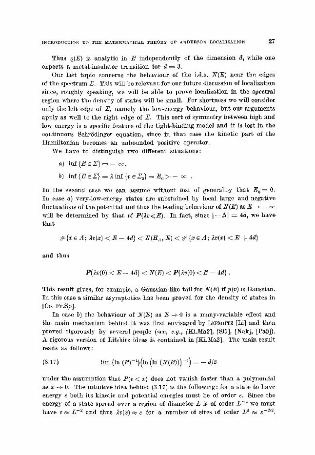
I n case b) the behaviour of N(E) as E -~ 0 is a many-va r i ab le effect and the main mechan ism behind it was first envisaged b y LI~SttITZ [Li] and then p roved rigorously by several people (see, e.g., [Ki.Ma2], ISIS], [Nak], [Pa3]). A rigorous version of Lifshitz ideas is contained in [Ki.Ma2]. The main result reads as follows:

(3.17) lira (111 (E) - I ) ( ln (ln (N(E))) -1) = - d/2

under the assumpt ion t h a t P(v < x) does not vanish fas ter t h a n a polynomia l as x -+ 0. The intui t ive idea behind (3.17) is the following: for a s ta te to have energy s bo th its kinetic and potent ia l energies mus t be of order e. Since the energy of a s ta te spread over a region of d iameter L is of order Z -2 we m u s t have e ~ Z -2 and thus 2v(x)~e for a n umber of sites of order L a ~ s -d/2.

2 ~ F. ) IARTINELLI a n d n . SCOPPOLA

Tiffs clearly happens with a p robabi l i ty of order

exp [ - - In (P(;,v < ~)-1) E-d/2].

4. - Proof of localization for large coupling constant through the analysis of the structure of the typical configurations of the random potential.

In this section we describe the s t ructure of the typica l configurations of the r~mdom potent ia l for large values of the coupling constant ). and we then

prove the exponent ia l localization of the eigenfunctions of H(v). To simplify the exposit ion, we will assume tha t the poten t ia l dis tr ibution satisfies the hypotheses A1 and A2 of sect. 2. The more general case in which only It:i, H2 hold will be discussed in appendix B and in sect. 7 for the one-dimensional

c a s e .

I n order to fix the ideas, we choose an energy E o in the spec t rum X which will be kept fixed th roughout all this section and we will invest igate the locali- zat ion propert ies of s ta tes %o of H(v) with energy in I - - [E o - 1, E o -~ :1]. F i rs t of all, there is a na tu ra l region in which u s ta te ~ with energy E e I mus t be localized. I f ~ c~u be normalized in such a w~y tha t

(4.1) I!~l!~ = sup I~(x)t = l ,

f rom the Schr6dingcr equat ion we obtain

(4.2) [;,v(x) + 2 d - - El 1~(~)1 < 2~ .

Therefore, the m a x i m u m of ~ is a t t a ined on the set {x~ Za; I2v(x)-~ 2d-- - - El < 2d} and in par t icular on the larger set

(~.3) So(Be, v) = (x; I;.v(~) + 2 ~ - - ~ot < ~/~}

provided tha t ~/~ is larger t han 2d + 1. Actual ly the localization of ~ oll S o is exponent ia l in the sense t h a t

(4.4) ly~(x) t < c exp [ - - m dist (x, So) ] , e > 0 ,

with m = In [(~/~/4d) -}- �89 > 0. Iu fact , on the complement of So, y~ is a solution of the Dirichlet p rob lem:

j (~(~,) - E) ~ = o in Z~ ' \So , (4.5) [ u r e S o = v .

Since b y construct ion dist (E, a(Hz~\s0)) ~ ~ / ~ - - 2d ~ 0, the above problem

I N T R O D U C T I O N T O T H E M A T H E M A T I C A L T H E O R Y O F A N D E R S O N L O C A L I Z A T I O N 2 ~

has a un ique solut ion g iven b y

(4 6) u(x) = w(x) = Y_, Gz,\~.(2~, x, y) v,(y') , x e ,~o. (v,v')e~So

The b o u n d (4.4) follows n o w i m m e d i a t e l y f r o m (4.6) if we observe tha~ t he

C o m b , s - T h o m a s a r g u m e n t of sect. 2 appl ied to Gz, \ s . (E , x, y) gives

(4.7) IGz,\s~ x, y)[ < cons t .exp [ - - mix -- Yl]

wi th m = in ['v/'X/dd -}- 1]. I n the a b o v e discussion we have a s sumed t h a t i t was possible to normal ize

in such a w a y t h a t II~01]~ = 1. ]Kowever, in order to get a b o u n d like (4.4),

all w h a t we rea l ly need is t h a t t he (possible) g r o w t h of yJ(x) as [x] -+ oo is less

t h a n an exponent ia l , s ince in this case express ion (4.6) can still be control led

by (4.7). As a l r eady expla ined in sect. 2, this is t h e case if t he ene rgy R of t he

s ta te ~o is ~ (~ genera l ized e igenvalue )) a nd ~p is the cor respond ing <~ general ized

eigerLfunction ,~.

W e now t u r n to discussing the local izat ion of ~ inside the r e l evan t sot S o.

This is rea l ly t he h e a r t of our discussion and it t u rns ou t to be a difficult

p roblem. The p robab i l i t y t h a t a g iven site, e.g. x ~ O, belongs to t he set S o

is v e r y smal l if 2 is sufficiently large; in fac t ,

(4.s) p ( o e go) = P(lav(o) + 2 d - ~ol < V ~ ) < c (V~) -~ ,

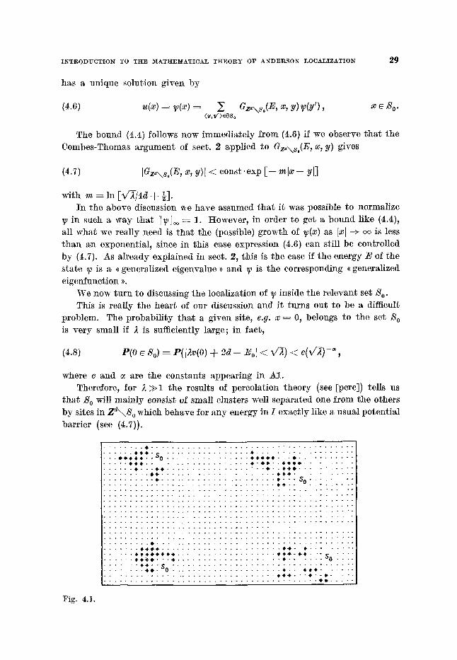
where c and ~ are the cons tan t s appea r ing in A1. Therefore , for ,I >>1 t he resul ts of pe rco la t ion t h e o r y (see [pore]) toils us

t h a t S o will m a i n l y consis t of small clusters well s epa ra ted one f r o m the o thers

b y sites in Z a \ S o which behave for a n y ene rgy in I exac t ly l ike a usua l po t en t i a l

bar r ie r (see (4.7)).

�9 . . . . . 4 . . . . . . . . . . . . . . . . . . . . . . . . " . . . . . . . . . . . . . . . . . . r . . . . . . . . . . . . . . . . * . . . . . . . . . . . . . . . . .

- . ~ * r 1 6 2 - ~0 * * o 4 , - . r - . . . . . . .

. . . . . . . . o * . . . . . . . . . . . . . . . . . . . . . ~ , 4 - . . . . . . .

. . . . . . . . . . . . . . . . . . . . . . . . . . . . . . . . . . . . . . . . o . . . . . .

. . . . . . . . 4 - o - . . . . . . . . . . . . . . . . . . . . . . . . . . . . . . . .

. . . . . �9 ******* . . . . . . . . . - . . - , ~ - - - - "" * * * ' + * " s o . . . . . . . . - * * ~ , - - - 4 . . . . . . . . .

. . . . . �9 4.. S . . . . . . . . . . . . . . . . . . . . . . . . . . . . . . . . . . .

. . . . . . ~ 0 - 0 . . . . . . . . . . . . . . . . . . . . . * - - * * 4 . . . . . .

. . . . . . . . . . . . . . . . . . . . . . . . . . . . . . . . . . . . . . . . 4 0 . . . . .

Fig. 4.1.

3 0 F . 5 [ A R T I N E L L I and E . S C O P P O L A

However , this fac t does no t imp ly au toma t i ca l l y the local izat ion of t he

wave func t ion h rj, since q u a n t u m - m e c h a n i c a l tUlm(qling effect m a y t ake place

leading to a delocalization of the s ta te a m o n g the clusters of S o. I n order to

i l lus t ra te the m a i n m e c h a n i s m which p reven t s such an effect, let us consider the

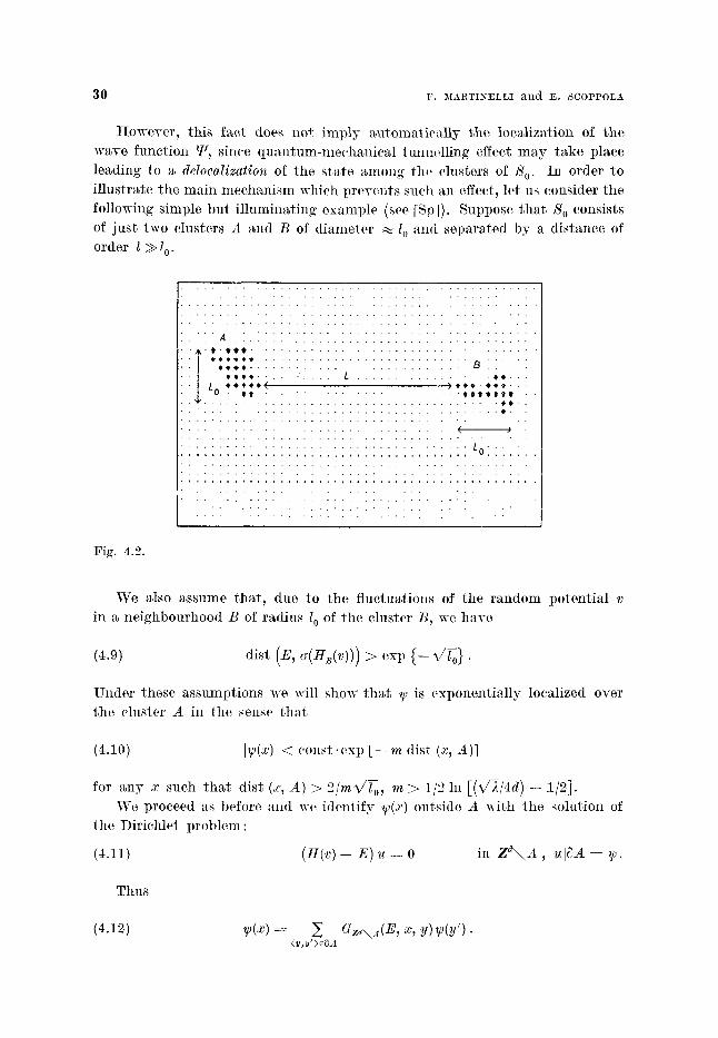
fol lowing simple bu t i l lumina t ing example (see [Sp]). Suppose t h a t S o consists

of jus t two clusters A and B of d i ame te r ~ l o mid separa ted b y a d is tance of order l >> 1 o.

Fig. 4.2.

A !I "~'0tt . . . . . . . . . . . . . . . . . . . . . . . . . . . . . . . . . . . . .

t r 1 6 2 ) * * * ' r " 0 " t t " �9 . . . . . . . . . . . . . . . t $ t t t e t "

. . . . . �9 . . . . . . . . . . . . . . . . . . . . . . . . . . . . . . . . r 1 6 2

. . . . . . . . . . . . . . . . . . . . . . ( )

: ; : : : : i l i . : : i ; : i i i : i ; : i l i : : : : ; . i i : i : : Lo: .

, , , . . . . . . . . . . . . . . . , . . . . . . . . . , . . . . . . . . . . . . . . . . .

1

W e also assume theft, due to the f luc tuat ions of the r a n d o m po ten t i a l v

in ~ ne ighbourhood B of radius l o of the cluster B, we have

(4.9) dist (E, > {--

U n d e r these assumpt ions we will show t h a t yJ is exponen t ia l ly localized over the cluster A in the sense t h a t

(4.1o) ]~f(x)] < c o n s t .exp [ - - m (list (x, A)]

for a n y x such t h a t dist (x, A) > 2/m~/~, m > 1/2 In [(~/X/4d) + 1/2]. W e proceed as before and we iden t i fy ~o(.r) outs ide A wi th the solut ion of

the Dir ichle t p r o b l e m :

(t.11) (H(c) -- E) u 0 in Z ~ A , ulnA = ~f.

Thus

(4.12) ~(x) = ~ Gz,\a(E, x, y)~(y'). (Y,V'>e~A

I N T R O D U C T I O N TO T H E M A T H E M A T I C A L T H E O I ~ Y OF A N D E R S O N L O C A L I Z A T I O N 31

The boundary t e rm at infinity vanishes because of the exponential decay of ~ outside S o.

Using the resolvent iden t i ty discussed in sect. 2, we write

(4.13) Gz~\.4(E, x, y) ---- GB,z~\A(E, x, y) ~ Gz,\AT'~GB.z, \A(E, x, y) ,

where F~ contains the couplings across the boundary of B. If now the site x in (4.13) is t aken inside B, then the first t e rm in (4.13) is zero and we can write

(4.14) GB.z~\A(E; x, y) = ~, Gz~\A(E, x, Z) Gz~\.4.~(E; z', y) . <z,z')e~.B

Using (4.4) the second factor in the sum (4.14) decays exponential ly in [ z ' - -y ] . The dangerous t e rm Gz~\A(E , x, z) can be controlled by the non- resonant condition (4.9) (see 1emma 5.2) b y

(4.15) IG~\~ (~ , x, z)i < eonst .exp [VVo] �9

Therefore, if we plug expression (4.13) into (4.12) we get (4.10). The above example is, of course r a caricature of the actual si tuation where

the set S o contains an infinite number of clusters. However, we learn two impor tan t things tha t are a t the basis of the subsequent results:

i) To prove exponent ia l localization of a generalized eigenfunction ~v with energy E in I outside a bounded region K c So(.Eo, v), it is sufficient to prove the exponential decay of the Green's funct ion Gz~\K(E, x, y) on the complement of t ha t region for I x - Y l sufficiently large.

ii) There can be regions intersecting the set So, like the set Z ~ \ A in the example, which behave on a sufficiently large scale like potent ia l barriers, t ha t is the associated Green's functions decay exponential ly fast.

The above two points suggest na tura l ly tha t the analysis of the localization properties of states with energy E e I could be successfully carried out if a sequence of length scales is in t roduced into the problems and the quantum- mechanical tunnell ing of the state ~v is studied separately on each scale. This program was implemented by JONA-LASII~IO, ]V~ARTINELLI and SCOP~'OLA [J-L. 1Vfa.Sc2] in the hierarchical version of the Anderson model, where the clusters were assumed to be arranged in such a way to give rise to a self-similar structure on a chosen sequence of length scales. We considered the scales in t roduced in [Fr.Spl] , given by

(4.16) d k = exp [fl(5/4)k], fl > 0.

We remark at this point t ha t other choices of the scales are possible provided tha t they satisfy the condition ~ dk/dk+ 1 < -~ ,:~.

k

32 F. MARTINELLI ~tnd E. SCOPPOLA

We will now expluin in detail how to apply the above gener~] idea to the

full Anderson model. We first need a name for the se~s of Z ~ which satisfy

ii) on scale d k.

De]inition. A set A c Z '~ is said to be a k-barrier for an energy E c I

with (( muss ~) me if

(GA(E , x, z)l ~ exp [--molX-- Yl], Ix - yl > (1/5)~,,

where d k is given by (4.16). As an exumple of a 0-barrier for uny energy E E I we can take an arbi t rary

subset of Z ~ S o , while, if we set in the previous example 1 = dk+l, l o ~- dk, then

any subset of Zd~A becomes a (k + 1)-barrier for the energy E. I t is now

clear t tmt one of the main problems is to find a constructive criterium in order

to decide whether a given region A is a k-burrier or not. This is a very dif-

ficult problem which can be solved only in u probabilistic sense. The first

impor tan t step in this direction was tuken by FRO~tLICH and SPENCER [Fr.Spl]

for a ]ixed energy E: they proved tha t for a fixed energy u given set A is a

k-barrier for most of the configurations.

Theorem 4.1 (Frohlieh, Spencer). Let the probubili ty distribution dP(v) satisfy A1, A2. Then there exists ~ ).o such tha t V), > ?.~ and any E c Z

P{v; A is not a k-barrier for E with mass roe>l~2 In (~/-~/2dd-1)}< [AI/d ~ with p = p(~) -~ -~ as ). -~ c~.

The above estimute was sufficient to prove the vanishing of the conduct ivi ty

at large disorder [Fr.Spl] and, us we showed in [Ma.Sc], the absence of an absolutely continuous component in the spectrum. However~ as we have already

explained in the discussion of the example, in order to prove localization in

some energy region it is importunt to decide whether u given region A is a

k-barrier not just for a ]ixed energy E e I but for the generalized eigenvalues o] H(v). This is a much more delicate problem since the generalized eigenvalues o] H(v) depend on the potential con/iguration v and they represent also the sup-

port of the spectral measure do(v) of H(v) which is singular with respect to the

Lebesgue measure with probabil i ty one [Ma.Se]. The solution to this problem

was provided by IFROItLICH~ ~[ARTLNELLI~ SCOPPOLA and SPENCER [Fr.Ma.

Sc.Sp] in the following form:

Theorem 4.2. Under the same,~ssumptions of theorem 1, for any 0 ~ y ~ 1/10 we have P{x; there exists un energy E ~ I such tha t A is not a/~-barrier for E

with mass m 0 and dist (E, (~(HA(V))) > exp [-- d~.]} < [A[/d~ (~), where p(~) is independent of ? and diverges to plus infinity as ~ -> ~ . Here

INTlC0DUCTION TO THE MATt IE~ATICAL TI-IEORY OF ANDERSON LOCALIZATION 3 3

Remark 1. I t is clear t ha t the above est imate becomes effective ouly for sets A such t ha t IAI/d~(~)<< 1 and diam A > dk/5 , since the p roper ty of being a k-barrier is seen only on a scale larger t han dk/5. Typical ly the est imate will be applied to sets A of d iameter of order dk+ I and A will be t aken so large tha t p(A) > 5[4. In this case the result is highly nontrivial because it applies to all energies E ~ I simultaneously and because the allowed resonance is ext remely small compared with the typica l spacing between the eigenvalues of HA(v ). This fact makes any a t t emp t to prove the above result by naive per turba t ion theory (e.g, the Combos-Thomas argument) bound to f a i l The proof of theorem 4.2 is pos tponed to sect. 6. while in appendix ]3 we indicate how to modify i t if the hypothesis ~ >>1 is replaced by the general assumption H1.

We have now all the tools to analyse in full detail the s t ructure of the typical configurations of the r andom potent ia l and to prove tha t t hey are such tha t the tunnell ing over too largo scales is forbidden for all the generalized eigenvalues E e l .

We introduce the sequence of boxes Ak, ~k centred at the origin and with sides of length [8d'~] and [dd~] respectively, where [-] denotes the integer par t . We also set

(4.17) A k = Ak"x.z~k_ I .

Then our main result reads as follows:

Theorem 4.3. There exists ~r > 0 such tha t for any ~ > ~r and any ~ < :1i10 there exists a set ~o c ~ of P-measure one with the following propert ies: for any v e ~o and any generalized eigenvalue E of H(v) in I there exist three integers kl(V), k2(v , E), ka(v ) such tha t

i) for any k > ki(v ) and any E e I , if z~ k is not a (k-- 1)-barrier for E with mass me, then dist (E, a(H2~_,)) < exp [ - - ~ - i ] and the same holds for

Ak+l;

ii) for any k > k2(v , .E), dist (E, a(H2,)) < exp [-- d~_l] and z~ k is not a ( k - - 1 ) - ba r r i e r for E with mass me;

iii) for any k > ka(v), dist (a(H~,§ a(H2,)) > 2 exp [-- ~ - l ] ;

iv) for any k > max {kl(v), k2(v , E), ks(v)} , A~+ 1 is a (k -- 1)-barrier for E with mass m o.

Hero m o is as in theorem 4.2.

Corollary 4.1 (Localization of the eigenfunctions). Under the assumptions and in the notat ions of theorem 4.3 for any v e ~o the generalized eigenfunctions of H(v) with eigenvalue E decay exponential ly fast at in i ty with (~ mass ~) m 0.

To state the nex t result we first define what we mean by the (( localization length ,; $(E) of an eigenfunction q with eigenvalue E. We normalize ~ in such

34 F. MARTINELLI and E. SCOPI~OLA

a way tha t sup I~<~)l = 1 and w e set M(E) = {x; l~<x)l = 1}. Then we define

(4.!8) ~(E) = m~x ra in{l ; 17(.r)l<exp[--mo[.r-xol/6]. V [ x - - x 0 1 > l } . x o e M ( E ) '

With this definition we have

Corollary 4.2. Under the assumpt ions of theorem 4.3,

P{3E; 0 ~ M(E) ~nd ~(E) > d~} < 1/d~ (~) .

Corollary 4.3 ((:ontrol of the t ime evolution). Le t PI(H(v)) be the spectral project ion of H(v) associated with I . Then for ), > ~r any v s Y20 and any

n r N there exists a constant C,(r) such tha t

{~ txl~'lexI ) [itH(v)] P,(H(v)) 8x 0(x)12} < C,(v), Vt > 0,

with fdP(v ) C,,(v) < ~ .

Before giving the fo rmal proof of the above results lot us explain in simple words their content . We s ta r t with theorem 4.3 on the s t ructure of the typica l

configurations.

i) says tha t , in order to decide whether the set Ak(A~.+~) is a ( k - - 1 ) - barr ier (of mass me) for a given eigenvalue E, we have olfly to check the s t rength of the resonance between the eigenvalue E and the spec t rum of the Hami l - tertian res t r ic ted to/ik(A~:+l ) provided t ha t the scale is large enough depending on the chosen configuration but ~ot on the given eigenvalue E. This un i formi ty in the energy is crucial in order to prove the remaining s ta tements .

if) is a very simple and intui t ive result if one believes in the exponent ia l localization of the states. Let us in fact pick a generalized eigenvMue /~ and le~ us suppose t h a t t.l~e corresponding eigenfunction decays exponent ia l ly fas t at infinity. Then it is clearly possible to find a scale k so large t h a t

(t.19) 5 I~(~)# > 1 - o (exp I-meal,,.]),

which in tu rn imphes t h a t

(4.20) dist (E, a(H~)) < exp [ - - d~_~].

iii) expresses a very weak nonresonance condition satisfied by a lmos t all potent ia l configurations v which together with i) and if) gives iv). As far as corollary 4.1 is concerned, it is clear tha t , if we replace the notion of k-barr ier with the more usual one of po ten t ia l barr ier v(x)> E, then the localization

of the eigenfunctions would follow immedia te ly .

INTRODUCTION TO THE MATHEMATICAL THEORY OF ANDERSON LOCALIZATION ~

In the course of the proof we will see t h a t the weaker not ion of k-barrier is ac tua l ly enough.

Corollary 4.2 requires no comments except t h a t i t is the first rigorous state- m e n t on the localization length (at least if this last one is defined as in (4.18)).

Corollary 4.3 is not such a s t ra ight forward consequence of corollary 4.1, since in general the only knowledge of exponent ia l decay of the eigenfunctions is not sufficient to control r igorously the t ime evolution. The new ingredient which is a by -p roduc t of our analysis is t h a t eigenfunctions with different

energies are localized in different regions of the latt ice.

W e now tu rn to the fo rmal proofs of these results.

Proo] el theorem 4.3.

i) Le t 2 be so large t h a t the power p(2) given in theorem 4.2 is larger

t h a n (5/4)2d. Wi th th is choice we see t h a t the p robabi l i ty appear ing in theorem 4.2 with A ei ther equal to ~k or to Ak+ I is summab le in k. Therefore, b y the Borel-Cantell i l emma (see sect. 2) there exists a set ~ i C ~ wi th

P(s ~ 1 and for every v e h I an integer kl(v ) such t h a t for any E e I , if ~k(Ak+l) is not a ( k - 1)-barrier of mass m o for E , t hen dist (E, ~ (H~)) <

< exp [ - - d~_i] (and the same for Ak+i) wi th 0 < ~ < 1[10.

ii) Le t v e A21, ~ being defined in the proof of i), and let us fix a gen-

eralized eigenvalue E e I of H(v). We suppose t ha t i t is possible to find a sequence k~ -+ + ~ of scales such t h a t nAk. is a ( k ~ - 1)-barrier for E. We will see t h a t this leads to a contradict ion. In each box Ak. we can ident i fy the generalized eigenfunct ion ~p associated wi th E with the unique solution of

the Dir ichlet p rob l em:

{Hj,,.(v) - - E} u : 0 in Ak.,

and thus we can wri te

(4.22) ~(x) : ~_, GA~.(E , x, y)y~(y'). <y,~ '>eOA~ n

I n (4.22) we can t ake x fixed and we let n -~ ~ . Since b y assumpt ion GA~.(.E, x , y ) decays exponent ia l ly for I x - - y l ~ (1/5)dk_ 1 and yJ increases a t mos t polynomial ly , we get

(4.23) ~0(x)-~ 0 for any x.

This shows that there exists an integer ]c2(E , v) such t h a t A k is not a (k - - 1)- barr ier for any k ~ k2(E , v). B y tak ing k2(E , v) ~ m a x (kl(V), k~(.E, v)) we get the final s t a tement .

36 F. MARTINELLI and E. 8COPPOLA

iii) This result follows again from the Borel-Cantelli lemma if we observe tha t the probabi l i ty of the complement of the event described in iii) satisfies the est imate

(4.24) P{dist (~(H&+,}, a(H&)) < 2 exp [ - -a~_l] } <

< [A~I 1~+~l(2 e~p [-d~_~])

and tha t the r.h.s, of (4.24) is summable in k. In order to get (4.24) we have used corollary 3.1 together with the statistical independence of the eigenvalues of H A f rom those H A .

iv) I t is an easy consequence of the first three. For any

k > m a x (~I(V), ]r v), ~3(v)) ,

i), ii), iii) occur simultaneously. Therefore, using ii) and iii),

(4.25) dist (E, (~(HA~+,)) > exp [ - - ~ - 1 ] ,

which, together with i), implies tha t Ak+ 1 is a ( k - 1)-barrier of mass m o for E.

_Proo] o/ corollary 4.1. Le t us fix a configuration v e ~o , ~0 being the set of measure one determined in theorem 4.3, let E be a generalized eigenvalue in I and let k~(v), k2(E , v), k3(v ) be the associated scale labels. Le t x be such that

(4.26) I~l > ma~ {d~l, G~, G,} .

A simple geometric a rgument shows tha t for such x's it is always possible to

find a scale d k such tha t

(4.27) x ~ Ak+ 1 and dist (x, Ak+l) > (1]3)Ix ] .

We now use (4.21) to express the generalized cigenhmction W associated with E at the site x in terms of its value at the boundary of Ak+ 1. We get

(4.28) y~(x) = ~, G 4~+I(E , x, y)yJ(y ') . <v, ~'}6~Ak+l

Note tha t by construct ion the Green's funct ion in (4.28) is evaluated at sites x, y with Ix-- y [ > (1/3)[x[ > (2 /3)dk> (1{5)d k. Therefore, since Ak+ 1 is a ( k - 1)-barrier for E and ~f grows at most polynomia]ly, (4.28) can be estimated by

(4.29) exp [ - - mo/3[x[Jl~Ak+ l[ < (J exp [-- moJXl/6 j .

INTRODUCTION TO THE MATHEMATICAL THEORY OF ANDERSON LOCALIZATION 3 7

The proof is completed.

Proof of corollary 1.2. Let s k be the set of configurations such tha t the following two conditions hold:

i) if ~ is not a (j -- 1)-barrier for E, then dist (E, ~(//A(v)) < exp [ - d~] for any j > k -- 1 and the same for A~+ l;

ii) dist (a(H~,(v)), a(tt~j+,(v))) > 3 exp [-- d~] for any j > k -- 1. Using theorem 4.2 and (4.24), we see tha t , if 2 >)1,

(4.30) P { a , } > 1 -

Suppose now tha t E e I is an eigenvalue of H(v) such tha t 0 e M(E). We will prove tha t $(E) > d k implies t ha t the configuration v is not in s k. In fact, for any ~ > 1, A~ is not a (j -- 1)-barrier for E since otherwise, using (4.22), [~o(0)[ would be smaller than uni ty. I f the configuration v is in ~k , t h e n b y construction the maximum of the three integers k~(v), k~(E, v), ka(v) introduced in theorem 4.3 iv) would be smaller than or equal to k -- 2, which in tu rn implies, by the proof of corollary 4.1, tha t

l (x)l < exp V- 0Ixl/6], Ix[ > dk_l,

i.e. $(E) < a,. Thus v e ~k and this, by (4.30), occurs with probabili ty less than or equM

to 1 / ~ (~).

1)roof of corollary 4.3. In order to control the t ime evolution of the initial wave packet Px(H(v))80, i t is natura l to expand the evolution operator exp [~ itH(v)] in terms of the oigonflmctions of H(v) and to exploit their exponential decay at infinity. For v e ~2o, where D o is the set described in theorem 4.3, we have

(4.31)

I

Here dpv is a spectral measure for it(v) (see sect. 2) and ~o~ is the eigenfunction with eigenvalue E. In (4.31) we have used the fact, proved by DELu LEVY and S0tm~LA~D [De.Le.Sou], t ha t the spectrum of H(v) is simple with probabili ty one. Le t now k(x) be the Iargest integer such t h a t dk(x ) < Ixl and let k0(E ) be the largest among the scale labels ki(v), ks(E , v) and ks(v ) introduced in theorem 4.3. With this notat ion we split the integral in (4.31) into two parts : one corresponding to those energies with ko(E ) < k(x) (i.e. energies whose eigenflmetions are localized inside a region of size ~ dk(~)_l < Ixl ~/5) and the

38 F. MARTINELLI and ~. SCOPPOLA

other corresponding to energies with ko(E ) > k(x):

(4.32) fdegE) exp [ - - i tE] ~vE(O )~vE(x ) = I

= f dQ~(E) exp [-- itE] ~(0) V+~(x) § f dev(E) exp [-- itE] wE(O) ~E(x). {E; ~0(~) < ~-(~:)} n Z (E; k0(E)> k(x)} n I

In the first integral the t e rm ~vE(0 ) ~z(x) can be est imated in absolute value using corollary 4.1 by

(4.33) const .exp I - m o l ~ - l ~ I " ~ l / 6 ] �9

To est imate the second integral, we make the following simple observat ion: if ko(E ) > k(x) and Ix[ is very large, then the eigenfunction ~v E will be localized outside a box centred at the origin of size a t least dk(:)_ 1 and thus the t e rm ~z(0) will be exponential ly small in dkc,.)_ ~. 5Iore precisely, if k(x) > max {k~(v), k3(v)} § I and if ko(E ) > k(x), then ko(E ) = ke(E , v). In tu rn this implies by the proof of theorem 4.3 tha t the box ~k0(E)-~ is a (ko(E)- 1)-barrier for E and thus, using (4.22) for x = 0, we get

(4.34) Iw~(O)l < exp [ -mod, o<~)/2] < exp [--molZl:~+::/23.

Estimates (4.33) and (4.34) show tha t for Ixl large enough (depending on the chosen configuration) the kernel {exp [-- itH(v)] Ps(H(v))} (0, x) decays faster t han any polynomial in Ix] with probabi l i ty one uniformly in the t ime t and the corollary is proved.

Remark. I t is actual ly possible to use the above argument combined with the probabilistic estimates of theorem 4.3 to show tha t also the expectat ion of the quant i ty { ~ Ix[~lexp [jtH(v)] Pz(H(v)) 8~=o(X)p} is uniformly bounded in the t ime t.

We conclude this section with a short discussion of the case +~ arb i t rary and E close to the bo t tom of the spectrum. According to the general scheme, we have to prove tha t H1 holds also in this case. We have to distinguish between two different cases:

a) i n f { E ; E + X } = - - c~,

b) inf {E; E e X} ---- ). inf {v ~ Xo} ---- 0 wi thout lost of generality.

h the first case (e.g., when the potent ia l distr ibution is Gaussian) we choose Eo<<0. Then for any E < E o we have

(4.35) ~ leA(E, 0, O)I = 2d/l~v(O) § 2d - - E l , [~] = 1

INTRODUCTION TO TI IE MATHEMATICAL THEORY OF ANDERSON LOCALIZATION 3 9

where A = {0} and ~A ~ {(0, y); lYl-~ 1}; therefore,

as E 0- ->~ ~ for any a ~ l . Thus, if E o << 0, the abo~-e probabi l i ty is ve ry small and tI1 applies. In the second case let us pick 1 >>E o ~ 0. Then, using the est imate on the

integrated density of states (3.17)~ one can show tha t

(4.37) P{a(HA,) n [0, 2Eo] -~ 0} < exp [-- cEodle],

where c is a constant and l ~ E o ~ (see [Ho.Ma] for a proof). Therefore, b y the Combes-Thomas argument , for any E < E o

(4.38) P( ~A IGA(E'x'Y)I>a for some x c A with dist(x,~A)>l/4)< y

exp [-- cEo ~12]

for any a such tha t E o ~ exp [ - - E o ~] ~ a ~ 1. Thus, if E o is small enough, t t l holds.

5. - Exponential decay of Green's functions: the Frohlieh and Spencer construction.

In this section we want to characterize in t e rm of the potent ia l config- ura t ion v the k-generalized potent ia l barriers in t roduced in the previous section. We recall t ha t a given region A of the lat t ice Z d is a k-barrier for a given energy E if

(5.1) leA(E, v; x, y)l<exp [-molx- Yl]

for any I x - - y [ >dk[5 , x, y cA, where {dk} is the set of scales in t roduced in (4.16).

The whole discussion is completely deterministic, the potent ia l config- ura t ion v being fixed once and for all, and it can be successfully applied to other nourandom models which present a scale s t ructure like the deterministic hierarchical potent ia l [J-L.)ia.Sc2]. As we will see, the s t ra tegy is quite close to the main ideas of the Kolmogorov, Arnold, ~ o s e r theorem on integrable systems in classical mechanics [Kam].

Le t us fix an energy E ~ X and in analogy to what we discussed in the previous section let the set BoA(E, v ) - So A be given by

(5.2) = (x c A; I v(x) + 2 d - - Et <

4 0 10. MARTIN:ELLI 9~Ild :E. SCOPPOLA

As a l ready shown in sect. 4, if V ' ~ > 2d ~- 1, then the Green 's funct ion a t energy E associated with the complement of S A decays exponent ia l ly fas t

with r a t e m o > In V]/(2d -~ 1) (see (4.7)). I f we now consider a region A such tha t So A r 0, i t m ~ y happen t h a t the

eigenvalues of H A are very close to E producing a ve ry small denomina tor in the Green 's function~ since

G~(E, v; x, y) = ~ T~, (x )T~, (y )[E, - - E] -~ . tg~ea(HA(v))

Let us come back to the example discussed in sect. 4 (see fig. 4.2), where the region So a consisted of only two clusters A and B of radius l o well isolated one from the other, i.e. dist (A, B) ---- l, />>/o, and recall t han B was in resonance with the energy E not more t h a n exp [--~/~o] (see (4.9)). This control of the resonance has been enough to prove the exponent ia l decay of the Green's func- t ion since the strong resonance admi t t ed was controlled by the exponent ia l

decay of the Green's function corresponding" to the H~mi l ton ian outside S o. The main idea in t roduced by FROHLIC~ and SPENCER is to repea t induc-

t ive ly the above a rgumen t over the sequence of length scales {dk}~C 1 in order to t rade the exponent ia l dcc~y over large scales for the exponent ia l decay on smaller scales. In order to do tha t , they consider a par t i t ion of the set So A into a sequence of regions C~ of increasing size and such t h a t the eigenvalues of the Hami l ton ian in these regions C~ are pe rmi t t ed to get closer and closer to E. The small divisors coming on scale d~ are controlled induct ively b y means of the exponent ia l decay of the Green's funct ion obtained on smaller scales as in the case of the example . Let us give some more detail of this induct ive technique.

We set

(5.3)

where

(5.4) S~'~(E, v) = U c;(E, v) c S~(E, ~) o~

j ~ 0, 1, ...,

is the subset of (( gentle singular sites of s t rength j }) of S A, defined as the max- imal union of components C~ sat isfying the following conditions:

Condition A(j):

i) d iam C~ < d~ ~ d(o ~/4), d o >>1,

if) dis~ (C~., S~C~.) > 2d~+1,

iii) dist (E, a(HD~(v)) ) > exp [ - - V ' ~ ] ,

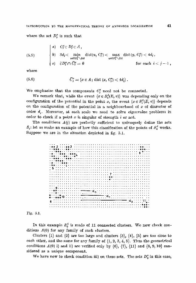
I N T R O D U C T I O ) / T O T H E M A T H E M A T I C A L T H E O R Y O F A N D E R S O N L O C A L I Z A T I O N 41

where the set D~ is such tha t

(5.5)

where

a) C~'cD~'cA,

b) 3d~< min dist(u, C?)< max dist(y, C~') < 4d~, v e ~ D ~ O A y e e D ~ A

c) ~ D ? ~ C ? ~ - - 0 for each i < ] - - 1 ,

(5.6) 0 ; -- {x E A; dist (x, C~) < 4d~}.

We emphasize t ha t the components C~ need not be connected We remark tha t , while the event {x ~ S'~(E, v)} was depending only on the

configuration of the potential in the point x, the event {x ~ sA(E, v)} depends on the configuration of the potential in ~ neighbourhood of x of diameter of order d~. Moreover, at each scale we need to solve eigenvalue problems in order to check if a point x is singular of strength i or not.

The conditions A(j) are perfectly sufficient to univoquely define the sets S~: let us make an example of how this classification of the points of So A works. Suppose we are in the situation depicted in fig. 51.

: ; ; 2 : : : ; ; 3 . . . . . . . . . . . . . . . . . . . . . . . . . . . . . . . . ~ �9 ~ , ~ . . - O � 9 . . . . . . . . . . . . . . . . . . . . . . . . . . . . . . . . . . 0 O O - - �9 - 0 0 0 . . . . . . . . . . . . . . . . . . . . . . . . . . . . . . . . . . . . . ~ �9 . - -

�9 " - ' 0 ~ 0 . - � 9 1 4 9 . . . . . . . . . . . . . . . . . . . . . . . . . . . . ~ . . . .

�9 0 0 0 . . . 0 0 0 . . . . . . . . . . . . . . . . . . . . . . . . . . . . . . . . . . . . . . �9 * 0 0 0 0 . . " . . . . . . . . . . . . . . . . . . . . . . . . . . . . . . . . . . . . . . .

�9 . . . . � 9 . . . . . . . . . . . . . . . . . . . . . . . . . . . . . . . . . . . . . . . .

5 . . . . . . . . . . . . . . . . . . . . . . . . . . . . . . . . . . . . . . . . . . . . .

. . . . . . . . . . . . . . . . . . . . . . . . . . . . . 7 . . . . . . . . . . . . . . . . . .

. . . . . . . . . . . . . . . . . . . . . . . . . . . . . 0 0 . . . . . . . . . . . . . . . . . .

. . . . . . . . . . . . . . . . . . . . . . . . . . . . . �9 . . . . . . . . . . . . . . . . . . .

: : : : : : : : : : : : : : : : : : : : : : : : : : : : : : : : : : : : : : : : : : : : : : : : :

�9 �9 : : : : : : : : : : : : : : : : : : : : : : : : : : : : . . . � 9 . . . . . . . . . . . . . . . . .

, . * ' : ; ; ~ 1 o : : : : : : : . . . . . . . . . . . . . ~1 . . . . . . . . . . . . . . . . . . .

. . . . . . . . . . . . . . . . . . . . . . . . . . . . . . . . . . . . . . . . . . . . . 0 0 � 9

. . . . . . . . . . . . . . . . . . . . . . . . . . . . . . . . . . . . . . . . . . . . . . 0 � 9

Fig. 5.1.

In this example So a is made of 11 connected clusters. We now check conditions A(0) for any family of such clusters.

Clusters {1} and {2} are too large and clusters {3}, {4}, {5} are too close to each other, and the same for any family of {1, 2, 3, 4, 5}. Thus the geometrical conditions A(0) i) and ii) are verified only by {6}, {7}, {11} and {8, 9, 10} considered as a unique component.

We have now to check condition iii) on these sets. The sets Do in this ease,

42 F. I~IARTIN]~LLI and 1~. SCOPPOLA

cr = {6}, {7}, {8, 9, 10}, {11}, can coincide with the sets C O because we have not to verify condition c) at step 0.

Suppose tha t condition iii) is only verified by the clusters {6}, {7} and {8, 9, 10}. We get, therefor%

S 1 = ~ 0 \ ~ 0 ~ = {1}, {2}, {3}, {4}, {5}, {11} .

Now {1, 2, 3, 4, 5} and {11} readily verify conditions A(1) i) and ii); in order to check the resonance condition iii), we have to be careful in constructing the set D(~ 1'2'3'4, 5} wi thout crossing the set C~ 7}. The choice of D~ ~'~'3'4'5} is not

unique, but this is not impor tan t since we are just interested in the fact t ha t there exists at least one.

As will be clear later (see appendix D), the resonance condition is almost independent of the choice of D~ in the sense tha t the change of a(Hz)(v)) , in the region near E, for different choices of D~ verifying a), b), c), is exponentiMly small (see corollary 5.4).

We remark tha t point iii) of condition A()) is given here, for teehnicM reasons tha t will appear clear later on, in a different way with respect to the original s ta tements of [Fr.Spl] , where D ~ - C~.

De/inition. A set D c A is k-admissible if ~ D ~ c A n C~ = O for any j = 0, 1, ..., k.

With this definition we have tha t the sets D~ are ( j - - 1)-admissible. The existence of admissible sets is ensured by the following lemma (see [Fr .Spl] for a proof).

Lemma 5.1. Le t D 1 C / ) 2 be rectangular regions in A such tha t

dist (D~, A~D2) > 10d~.

If d o is sufficiently large there is a k-admissible set D such tha t D1 c D c D 2.

We now come to the mMu s ta tement of this section.

Theorem 5.1. For 2 sufficiently large and a rb i t ra ry s there is a constant m = m(X) such tha t , if A is a k-admissible set ia A and

then

A A n Sk+I(E, v) = 0,

[GA(E + i~, v; x, Y)I < exp [-- mix - y[]

provided Ix-- y[ > dk+l/5. The (~ mass )) m(2) is independent of A and k ~md it is es t imated by m(2) >

> ll,~[m (VAI(~ + 1))].

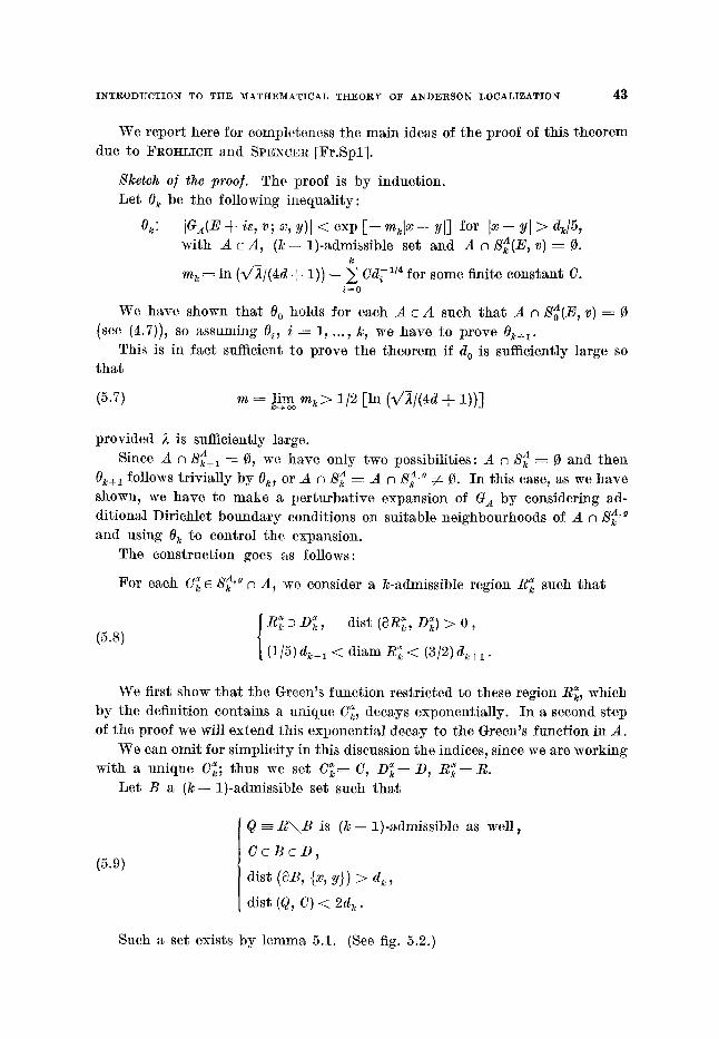
I N TRO D U CTI O N TO THE MATHEMATICAL THEORY OF ANDERSON LOCALIZATION ~ 3

We repor t hero for completeness the main ideas of the proof of this theorem duo to FR0~LIOE and SPENCER [Fr.Spl] .

Sketch el the pro@ The proof is by induction. Le t 0 h be the following inequal i ty:

Oh: IGA(E+ie , v ; x , y ) [ < e x p V - m ~ l x - y ] ] for [ x - - Y i > d h / 5 , A with A c A, (k -- l)-admissible set and A n S h (E, v) ~ O.

h

m h = In (V/~/(4d + 1)) -- ~ Cdi -1/4 for some finite constant C. i = 0

We have shown tha t 0 0 holds for each A c A such tha t A n S~(E, v) ~ 0 (see (4.7)), so assuming 0i, i --~ 1~ ...~ k, we have to prove 0h+ ~.

This is in fact sufficient to prove the theorem if d o is sufficiently large so tha t

(5.7) m = ~im m h > 1/2 [ ~ (V]I(4~ + 1))]

provided 2 is sufficiently largo. A Since A n Sh+ 1 ~- O, we have only two possibilities: A n S~ ~-- 0 and then

A~g 0~+~ follows tr ivial ly by 0h~ or A n S A ~ A n S h ~: 0. In this case~ as we have shown, we have to make a per tu rba t ive expansion of G A by considering ~d- dit ional Diriehlet boundary conditions on suituble neighbourhoods of A n S A'g and using 0 h to control the expansion.

The construct ion goes gs follows:

For each C~ ~ S~ 'g n A , we consider a k-admissible region R~ such tha t

(5.s) { / ~ ~ D~, dist (~R~, D~) > 0,

(1/5) dh+ 1 < diam R~ < (3/2) dh+ 1 .

We first show tha t the Green's funct ion restr icted to these region tt~, which by the definition contains a unique C~, decays exponential ly. In a second step of the proof we will ex tend ~his exponential decay to the Green's funct ion in A.

We can omit for simplicity in this discussion the indices, since we are working with a unique C~; thus we set C~= C, D~----D, /~--~ R.

Le t B a ( k - 1)-admissible set such t ha t

(5.9)

Q - R \ B is (k -- 1)-admissible as well

C c B c D ,

dist (eB, {x, V}) > dh,

dist (Q, C) ( 2d k .

Such a set exists by lemma 5.1. (See fig. 5.2.)

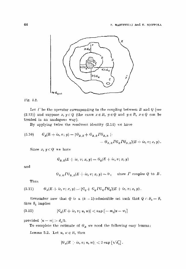
~ F. MARTINELLI and E. SCOPPOLA

. . . . . ~ k R

( Fig. 5.2.

Le t F be the operator corresponding to the coupling between B and Q (see (2.13)) and suppose x, y e O (the cases x e B , y e Q and y e B, x e Q can be t rea ted in an analogous way).

B y applying twice the resolvent ident i ty (2.14) we have

(5.10) GR(E ~- ie, v; y) : [G~. R 4- GB, nFGB,~ -~

~- GB.nFG~FG~.n](E -~ is, v; x, y ) .

Since x, y e Q we have

GB, R(E ~- is, v; x~ y) : GQ(E ~- ie, v; x, y)

and

G~,~I'G~,R(E -~ is, v; x, y) ~- 0 , since / ' couples Q to B .

Thus

(5.11) GR(E ~- ie, v; x, y) ~-- [GQ ~- GolVGRFGo](E-~ ie, v; x, y) .

Remember now tha t Q is a (k- -1) -admiss ib le set such tha t Q n S k : 0, ~hus O k implies

(5.12) [GQ(E + is, v; u, w)[ < exp [-- mk[u -- wt]

provided lu- - w I ~ dk/5. To complete the est imate of G~ we need the following easy lemma:

.Lemma 5.2. Le t u, w c B, then

IGn(E -~ is, v; u, w)] < 2 exp [Vd~k] �9

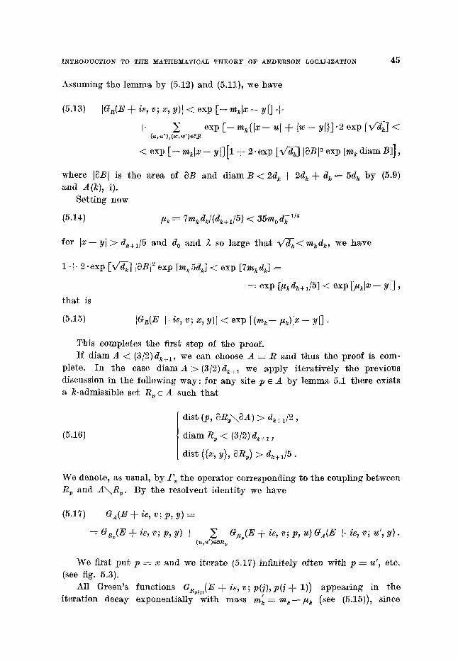
INTRODUCTION TO THE MATHEMATICAL Tti-EORY OF ANDERSON LOCALIZATION ~

Assuming the lemma by (5.12) and (5.11), we have

(5.13) IGR(B + is, v; x, Y)I< exp [-- ~ l x - - Y I] +

+ Z e~p [ - ~ { [ x - ~[ + Iv - u[}]'2 exp EV-a-;] < (u,u') , (w,w')~

< exp [--mk]x-- yl][1 + 2 .exp [ V ~ ] ]~BI: exp [m~ diam B]],

where [~B I is the area of ~B and d i a m B < 2 d k ~ - 2 d ~ + d ~ 5 d ~ by (5.9) and A(k), i).

Setting now

(5.14=) f ~ = 7m~ d~/(dk + ~/5 ) < 3 5 m o d ~ 1/~

for [x--Y] > dk+~/5 and d o and 2 so large tha t V/~<mkdk , we have

1 + 2 .e~p [ V ~ ] I~BI ~ exp [m~5a~] < exp [Tm~a~] =

- - exp [/~ka~+~/5] < exp [/~klz - y[] ,

tha t is

(5.~5) I ~ ( E + i~, v; x, y)] < exp [ ( ~ - ~ ) [ x - y l ] .

This completes the first step of the proof. If d i a m A < (3/2)dk+1, we can choose A = R and thus the proof is com-

plete. In the case d i a m A > (3/2)dk+ ~ we apply i teratively the previous discussion in the following way: for any site p e A by lemma 5.1 there exists a k-admissible set Rvc A such tha t

(5.16)

dist (p, ~ R ~ A ) > dk+l/2 ,

diam R~ < (3/2) dk+ 1 ,

dist ({x, y}, ~R~) > a~+1/5 �9

We denote, as usual, by F~ the operator corresponding to the coupling between R v and A~Rv . By the resolvent ident i ty we have

(5.17) G A(E ~- is, v; p, y) :

= GR~(F~ + is, v; p, y) + ~, G~,(E + is, v; p, u) GA(E + ie, v; u', y).

We first pu t p ~ x and we i terate (5.17) infinitely often with p ---- u', etc. (see fig. 5.3).

All Green's functions GR~(,(E+ie, v ;p( j ) ,p ( jd-1) ) appearing in the i terat ion decay exponentially with mass m' k ~ mk--/x k (see (5.15)), since

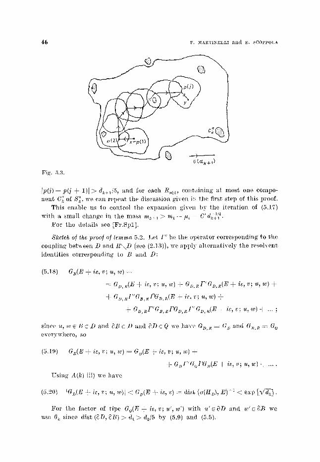
46 l~. 1M:ARTINELLI BAld E . S C O P P O L A

~(~+~)

Fig. 5.3.

[p(j) - - p(j 4- 1)[ > dk+l/5 , alId for each Rv(j), cont~Sning at mos t one compo- ne, n t C~. of S~., we can repent the discussion given iI~_ the first step of this proof.

This enable us to control the expansion givel~ by the i tera t ion of (5.17)

with ~ small change in the mqss mt :-1 > ink-- # ~ , - C"~-~/4 ~kq-1 "

For tho deta.ils see [Fr .Spl] .

Sketch of the proof of lemma 5.2. Let F ' be the opera tor corresponding to the coupling between D ~nd R ~ D (see (2.13)), we apply a l te rna t ive ly the resolvent

identi t ies corresponding to B ~nd D:

(5.18) Gn(E 4- i~, v; u, w)

~- Gg,~(E q- i~, v; u, w) 4- G~,nF'GD,~(E -~ is, v; u, w) 4-

4- GD, RFG~,RFGD,~(E 4- is, v; U, w) q-

G~,RF'G~,RFGD,nF' GD,R(E 4- i~, v; u~ w) 4- ... ;

since u, ,w ~ B c D a, nd 8B c D :~nd 8 D c Q w e h a , ~ G1),n ~ G o a.nd GB, n ~ G o everywhere , so

(5.19) Gs(E 4- is, v; u, w) : G1)(E ~ is, v; u, w) 4-

4- GDF'G(~FG~(E 4- is~ v; u, w) q- ... .

Using A(k) iii) we ha.re

(5.o~0) I e . (E § i~, ~,; u, ~)1 < C~.(E § i~, ~) = dist (~(H.), E) -1 < exp I V a n .

For the fac tor of ripe G~(E 4- is, v; u', w') with u ' c c~D and w ' c ~B we use 0 k siace dist (~D, ~B) > d~ > dd5 by (5.9) and (5.5).

INTRODUCTION TO THE MATHEMATICAL THEORY OF ANDERSON LOCALIZATION ~ 7

With these exponential ly small terms and with (5.20) it is easy to control (5.19).

We finally s ta te two corollaries which we will need la ter (for the proofs see appendix D):

Corollary 5.1. For any set A c A satisfying hypotheses

sup la~(E + i~, v; x, Y)I < 3 .exp [ C ~ ]

uniformly in s.

Corollary 5.2.

of theorem 5.2

Le t C c S~ satisfy conditions A(j) i), if) bu t not iii). Then

dist (E, a(Hs)) < exp [ - - V ~ / 3 ] ,

where C ~ {x ~ A; dist (x, C) < 4d~}.

6 . - P r o b a b i l i s t i c e s t i m a t e s .

We divide this technical section devoted to the proof of theorem 4.2 in three subsections. In the first one we review a geometrical construction first in t roduced by FROHLIC~ and SPENCE~ in their work on the Koster l i tz and Thouless t ransi t ion in the Coulomb gas [Fr.Sp3] and subsequently used in their proof of theorem 4.1 which Mlows us to est imate the (~ combinatorial en t ropy ,) of subsets of a region A.

In the second par t we give the proof of the probabilistic est imate by means of several technical lemmas which will be proved in the last subsection.

6"1. Notations and combinatorial results. - Let Zd(n) ~- 2 " g d, n > 0. Wi th each site j ~ Zd(n -- 1) we associate a cube C,(j) with sides of length 2" parallel to the latt ice axes and centred at j. Each Ca(j) will be called a n-cube. For n = 0 we set g d ( - 1 ) ~ Z ~ and a 0-cube is a site in Z ~.

Given a set D c Z d we define ~ , (D) to be a minimal family of n-cubes (i.e. the eardinal i ty ]~',(D)t is minimal) which cover D.

The volume of D on scale 2" is

(6.1) V.(D) == IV.(D)I, Vo(D) =-- IDI

and the to ta l volume no(D)

(6.2) V(D) ~_ ~ Vn(D) , n = O

where

(6.3) no(D ) -- rain {n ~ N; 2 ~ > diam D},

4 ~ F. MARTINELLI a n d :E. SCOPPOLA

tha t is the smallest integer such tha t D is covered by a single n-cub% s o 2n~ < 2 diam D.

Example. Let D be made of two points separated by a distance Z; then, V,~(D) = 2 for all n such tha t 2 " ~ L. Thus

V(D) ~ 2 log 2 L .

More generally, since V,(D) ~ 2 for all n < no(D), no(D ) < log 2 (diam D) .const , we have

(6.4) V(D) > log (diam D). eonst .

An impor tan t notion is that of (~ isolated cubes ~. We define for any set D c Z d

(6.5) T ; ( D ) = {C c cal,(D); dist(C, C') > "2.'z s'/~ for all C '6 (d,(D), C ~= C'}

no(/)) V'(D) ~',~{D)I, V'(D) ~ ~ V'(D).

~ l = 0

The basic combinatorial results (entropy estimate) are the following (see [Fr.Spl], [Fr.Sp3] for the proofs).

Theorem 6.1. If N(V) is the number of subsets D c Z ~ with 0 e D ~nd V(D) = V , then

N(V) .< exp [KdV],

where K a is a d-dependent constant. l

Theorem 6.2. There exists a constant K d only depending on the dimension d such tha t V(D) < K'd(ID I -+- V'(D)) for all D.

6"2. Proo/ el theorem 4.2. - In the previous section (see theorem 5.2) we

saw tha t a sufficient condition in order tha t a given region A c Z a be ~ k-bari%r

of muss m 0 > (1/2) In (~/-2/2d) is tha t the k-singular set SA(E) be empty. Thus

we can estimate the probabil i ty appearing in theorem 4.2 by

(6.6) P(v ~ ~ ; 3E c I such tha t S~.(E) =/- 0 ~nd

dist (E, > exp E--d;m) .

The next impor tan t step consists in showing tha t the condition

dist (E, > exp E--d;/3]

in (6.6) imposes a strong restriction on the structure of the set SA(E).


Essential ly S~(E) will not have in our case too small components well isolated f rom the rest on a scale close to d k. More precisely, using the notion of isolated cubes in t roduced in the previous subsection, we will prove

.Eemma 6.1.

P(ves 3 E e I

where

such t ha t S~(E)=/: 0 and

P(v ~ ~2 ; 3.E ~ I such t h a t S~(E) # 0 and

/ A ~'n(Sk(E)-~ 0 for any n such t h a t

n(r, k) < n < n+(k) and diam S~(E) > 2~+(k)-1),

n+(k)=max{neN;2n<dk_~} , n_@, k )=min{ neN;2">d~ r} .

Next we decompose the event appearing in lemma 6.1 into the union of events labelled by subsets of the region A each of which is such tha t the random set S~(E) associated with a given potent ia l configuration v is somehow localized in space. The probabi l i ty of the to ta l event will be then est imated b y the sum of the probabilit ies of each subevent. This ra ther crude procedure is sufficient for our purposes for large disorder 2 or more generally if H1 holds (see appendix B).

Zemma 6.2.

(6.7) P ( v e ~ ; 3 E e I ; S A ( E ) r 0, diamS~(E)> 2 "+(k)-l, and

r A v . ( s~(~) ) = 0, w e (~_(~, k), ~+(k)) a N) < Z P~,

where

N k ~ {D c A; diam D > 2 '~+(k)-l, c~:(D) = 0, Vn > n @ , k), n < no(D)}

and

P~ _= P(~ ~ a ; ~E ~ Z; S~(E) ~ D and dist (D, S~(E)\D) > 2.2~*(~)~).

The easy proofs of these two lemmas are given for completeness in the following subsection.

At this point the main idea to es t imate P• is to associate a small factor exp [--~/d~(~i/3], with j(n) defined by

(6.8) ~(n) ~ min {i e N; d~ > 2"}

for each couple of isolated cubes (C, C') ~ ~'~(D).

~ 0 F. ~r a n d :E, 8COPFOLA

In fact, as we will show in the course of the proof of lemma 6.1, each isolated cube C e <~:(D) satisfies the geometrical conditions A(](n)) i), ii) of sect. 5. Therefore, if j(n) < k and since C n D c SA(E), the crucial nonresonunt condit ion A(j(n)) iii) must be violated for the energy E.

Thus, if g',(D) consists of at least two cubes, then the above argument plus the t r iangular inequal i ty imply ~hat for each couple C, C' in g~'(D) one has

dis t ( ( < e (r He',r)), .exp [-- ge/(n)/3]

I t is impor tan t to observe tha t (6.9) is independent of the energy E. In other words, by considering resonances between different cubes in ~'n(D) we have overcome the problem of having an uncountable set of energies in our main event.

A simple use of coroll,~ry 3. l, together with the statist ical independence of the potent ia l in different sites, implies tha t the above event {6.9) has a very small probabi l i ty of order exp [--a~/dj(+,)/3].

Using this idea we will prove

Lemma 6.3. If ~ is sufficiently large, for each D ~ ~ .

PD< exp [ - -Ko[ ID 1 + V'(D)]] .exp [K o # {n<no(D); [~[~(D)l =/= 0}],

where W(D) is given by (6.5) and K o ~ K0(,~ ) is a constant which tends to infinity as ,~-~ ~ .

With this result we can now estima.te the sum over D ~ ~k of PD:

(6.1o) exp [-- KotD I -- K o V'(D) + K o # {n<no(D); ~'~(D) =/= 0}] <

< ~ exp [ - - K o l D I - K o V'(D)/2] d- {D~@~; V'(D)~2#{n<no(D);~(D):O)}

d- ~ exp [ - - K01DI] , (De~k; V'(D)<2# (n<no(D);~.(D)r

since obviously V'(D) > # {n<no(d); <d'.(D) =A 0}. The first sum in the r.h.s, of (6.10) is est imated by

(6.11)

where

~ ~ exp [-- Ko[ID I -~ V'(D)/2]], xeA V De...,~k(V,x)

~k(V, x) ~_ {D c A ; D e x, diam D ~ 2 +~+(k)- ~, V(D) ~- V}.

I N T R O D U C T I O N TO T H E ~ I A T H E M A T I C A L T H E O R Y O F A N D E R S O N L O C A L I Z A T I O N

By theorems 6.1 and 6.2 and using inequality (6.4), we get that

2 2 2 xeA V De.@~(V,~)

51

exp [--Ko[ID[-+- V'(D)/2] <

< ~ ~ exp [-- K o Vl2K'a] exp [K a V], xeA V < c o n s t ' l n (2n+ - I )

! which, for ~ so large that K0(2 ) > KaKa, is bounded by

(6.12) [A] exp [-- Ko(2) In 2 n+(k)-l]

with K:0(2 ) which tends to infinity as ~ -+ oo. Using the definition of n+(k), this implies the bound

(6.13) IAICla~ ~(~)

for some constant C1 independent of k with p which tends to infinity as )t tends to infinity.

In order to estimate the second term in the r.h.s, of (6.10), we write

(6.14) Z Z oxp [-- Kro] Z 1. ~eA Vo D ~ , x e D , [ D [ = go

W(D) < 2/] { n < no(D); (Tn" (D) r 0}

Zemma 6.4. Let D e ~ be such that V'(D) < 2. #{n < no(D); ~j(D) # 0}. Then

IDI > const .In dk_ I

provided y is small enough.

With this lemma (6.14) is bounded by

(6.15) [Al 2 exp[--gvo]#(De~k; r'(D)<2#{n<no(D); v~(n)#o}, Vo> const-ln dk- i

IDI = v0, O D).

Using again theorems 6.1 and 6.2, we have

(6.16) # { D e ~k; V'(D)<2"#{n<no(D);W', ,(D)#O}, IDI= Vo, oeD}< < 2 exp [K d V] < exp [Kd(V o + n_(y, k))]

V <<. K~(Vo+ ~.~_(r,k))

for some constant K a depending only on the dimension d. Inserting (6.16) in (6.15) and taking ~t sufficiently large, we obtain that

(6.15) is bounded by

[A[C2d~ r

with p'(~) which tends to infinity as ~ --> oo. The proof is complete.

5 2 F . M A R T I N E L L I and E . S C O P P O L A

6"3. Proof of the lemmas.

Proof of lemma 6.1. Firs t assume that there exists E ~ I such tha t SA(E) va 0 A and ~n(S~ (E)) ~: 0 for some n e (n_(~, k), n+(k)) n N.

t A For each cube C ~ ~n(Sk(E)), the set C n S~(E) satisfies the geometrical conditiorrs A(j(n)) i), ii) with j(n) given by (6.8).

Ill fact, by the definition of isolated cubes we have

and

diem ( C n SA(E)) < 2" <di(,)

0 . , / 5 / 4 _ _ dist ( G, S~(E)~ C) > 2.2 ~5/3 > 2.2 ~/~~ > ,, ~j(~) - 2 .dj(~)+ ~ .

Therefore, ill order to have C n S~(E) =/= 0, the spectral condition A(](n)) iii) must have been violated since j(n) < k, Vn e (n_, n+), i.e. using corollary 5.2

(6.17) dist (H@~(v), E) < exp [--V~-~(,i/3],

where

C n SA(E) -- {x ~ A ; dist (x, C n SA(E)) < 4d~(,)}.

By the definition of n_@, k) for all n > n_@, k)

exv [ - v/~:~)] < exp 1 - d~J.

I t is not difficult to prove (see the remark in appendix D) tha t this implies

(6.~s) dist (~(H~(v)), ~) < exp [ - d~/3j,

' A Therefore, we can assume that , for al l /~ e I such tha t S(E A) # O, ~ ( S k (E)) = 0 for any n E (n @, k), n+(k)) n N.

This iu turll implies tha t for such energies diam SA(E) > 2 ~§ otherwise ~',+(k)_I(SA(E)) would be nonempty .

Proof o/ lemma 6.2. We have to show tha t , if the event described in the

S k (E) in ~k- 1.h.s. of (6.7) is verified, then we can find a set D c A Le t

%(s~ (E)) ~ 0} (6.19) n'(k) ~ min {n > n+(k); ' A

~nd let

A ! D ~ S k (E) n C~,(~) for an a rb i t ra ry cube C~r ) c (d,~,(k) .


We observe that the definition (6.19) is nonempty since diam SA(E) ~ 2 ~+(k)-l. We will show that D belongs to ~k.

In fact,

(6.20) diam D > 2 ~'(~)-1 ,

otherwise U' ~'(k)-l# ~; moreover7 no(D)= n'(k) by construction and by the definitioa of n'(k)

, A vn e ( n ( ~ , k), n'(k)) vn(s~(~)) = ~ ,

This implies the same relation for D.

Proof o/ lemma 6.3. We define

(6.21) J~d'D(V) -- 9E'(V e ~ ; 3 E e I ; sA(E) c D and

dist (D, S~(E)~D) > 2.2"+(~)5j3),

where ~ ( . ) denotes the characteristic function of the event (.). Let n > O and suppose IU:(D)] > 17 for each C, C ' e U:(D) we define

(6.22) ~n,v,v,(v) ~--

Let ~Co, ~ be the characteristic function of the event that x e S~(Eo) , that is

~o,~(v) = :v(~ e ~ ; Iv(x) § 2a - Eel < V]).

i A By the proof of lemma 6.1 (see (6.17))7 for each couple C7 C' e U~(Se) with n < n+(k) we h~ve

(6.23) dist ((~(H~(v)) n I, (~(H~h(v)) ca I) < 2.exp [-- d~(,) /3].

This implies with the previous notations that

(6.e4) ~ < 1-I I-[ I ] ~ ,o ,o , (~) . x e D n; ] ~ ( D ) ] > I V,G'eeff~(D)

C r

To prove (6.24) we observe that triviaDy all the points of SA(E) must be points of S~(Eo) 7 moreover, each couple C, C' e U:(D) with n < n_(r7 k) belongs

r A also to Un(S k) since dist (R 7 S~(E)~D) > 2.2~+(k)5/~> 2.2 ~5/3. Thus, using (6.23)7 (6.24) follows.

5 4 P. MARTINI~LLI ~ n ~ 1~. SCOPPOLA

To est imate the expectat ion of the r.h.s, of (6.24)) we use the Holder inequal i ty and the independence of the random variables v(x), x ~ D. We get

(6.25) PD < [ ]-[ f~o~(v)dP(v)] 1-'" x 6 D "~ �9 a

H n; tY;,(D)I> 1

where r e (0, 1).

~ r t~nlr"(i-r) ,

G # C "

~ e x t we observe t ha t for a fixed C c W:(D) the characterist ic functions 3t',, c, c'(v) as a function of the configuration of the potent ia l in C' ~re statist ically independent for the different C"s in (d',(D), since for each C1, C 2 in C',~(D)

dist ( C1 ~ D, C2 m D) > 2 .2 ~ / ~ - 2" 4dj(,)> 2 .2 '~s /a- 8.2'~5/4 > 0 .

This implies by the product s t ructure of the measure dP(v)

(6.26) fdP(v) 1-[ ~..~,c.(v) = C, r

C~C '

=f 1-[ [I Ce~"n(D) x e g o D

xEC' o n D

dP(v(x)) [ [ ~.,o,~,(v) < e'~tc~(/))

G'# (~'

dP(~(x)) I] 1-[ dP(~(U))X..~~ C'ecg', ,(D) v ~ C ' n D

C ' # G o

where C O is an a rb i t ra ry cube in r

Each form f I-I dP(v(Y))JT~,,Vo,V'(v) is Y~G' a D

x ~ Co n D , using corollary 3.1, by

est imated uniformly on v(x))

(6.2~) f 1-I yeC," n D

4P(v(y)) ~,,Co,C,(v) < (1/2~)-2. (5d~(,))2a'exp [-- a Vd~(~)/6],

~ > 0 .

Combining (6.27), (6.26) and (6.25), we obtain

(6.28)

�9 ,: ~ > ~ > i [(~/~,o). 2. (~(,>)~. exp [ - ~ , / ~ / 6 1 ] " ' ` ' - ' > ( ~ ( ~ .

Choosing now r--~ 0.8 > 1/~/~, the t e rm

[(11i ~) -2 �9 (5~(.))~. exp [ - ~Vd~(,,>/6]] "~


can be made arbi t rar i ly small for ~ large uniformly in n, since

~/ds(~)r~> ( v ~ - r ) ~ > C ~ with C > : l .

F rom this i t easily follows tha t for ~ sufficiently large there exists a constant

K o ~ Ko(~ ) which tends to infinity as 2 - + ~ , such tha t

P1)<exp[--KoiDI] 'exp[--Ko Z (I~'~(D)I-- x)] �9 {n<n0; [~;,(D)l r 0)

The lemma is proved.

Proo] el lemma 6.4. By theorem 6.2 and (6.4) we have

cons t . ln (diam D)< V(D) < g'd(ID ] -~ V'(D)) <

<K'~([D I ~- 2. #~ (n < n0(D); (~:(P) ee 0}) < g'd(IDI-{- 2 n ( ~ , k)) ,

since D e ~k and V'(D) < 2. ~ (n < no; ~ ' (D) :/= O}. Moreover, we have tha t

diam D ~ 2 ~+(k)-I ,

thus

[D[ > c o n s t - ( n + ( k ) - 1 ) - 2 . n ( 7 , k)/K'~.

For 7 small enough we obtain

ID[ > const .ln (dk_l).

7 . - T h e o n e - d i m e n s i o n a l c a s e .

In this section we propose to unders tand the one-dimensional Anderson model within our approach. This case has been analysed since a long t ime and most of our results will not be new; however, we feel i t worthwhile to present a new point of view on the problem, since, for example, i t allows one to control the interest ing case of a binary alloy which has been so far out of reach of the s tandard approaches.

The idea, as already explained in the introduct ion, is ve ry simple and na tura l : the system when looked upon on a sufficiently large scale behaves like a weakly coupled system which should be, therefore, within reach of per turba t ion theory. The mathemat ica l character izat ion of weak coupling is given in our main hypothesis H1. Thus our aim is to verify H1 and H2 for all energies and all positive values of the disorder 2. Before doing tha t , let us, however, make ~ sort of scale t ransformat ion which we hope might clarify our

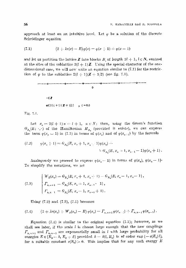
5 6 F . 5 f A R T I N E L L I a n d n . S C O P P O L A

approach at least on an intui t ive level. Let ~ be a solution of the discrete Schr6dinger equat ion

(7d) (2 4- 2v(x) - E)q~(x) = q~(x 4- 1) 4- q~(x - - 1)

and let us par t i t ion the latt ice Z into blocks B~ of length 21 4- 1, l ~ N, centred at the sites of the sublatt ice 2(I 4- 1)Z. Using the special character of the one- dimensional case, we will now write an equatiou similar to (7.1) for the restric-

t ion of q~ to the sublatt ice 2(l 4- 1)(Z 4- 1/2) (see fig. 7.1).

. . . . . . . . . . ~ . . . . . . . . . . . . . . . . . Q . . . . . . . . . . . . . . . . . GI . . . . . . . . . . . . . . . *"~*~176 . . . . . . . . . . . . . . "J . . . . . . . . . . . . . . . . . i ] . . . . . . . . �9

0

.EZ

QE2(L +1) (Z-'F 1/2) ~L=8.0

Fig. 7.1.

Le t x ~ = 2 ( l ~ - l ) n - ~ 1 4 - 1, n 6 N ; then, using the Green's funct ion GB.(E; . , . ) of the gami l ton inn HB. (provided it exists), we can express the te rm ~(x~ ~ 1) in (7.1) in terms of ~(xn) and of ~(x~,+~) by the formula

(;2) ~(x,, + 1) = Gs.(E , x,, + 1, x,, + 1)~{x,,) 4-

4- GB,,(E , x,~4- 1, x,+ 1 -- 1)?(xn 4- 1) .

Analogously we proceed ~o express ~v(x,~-- 1) in terms of ~v(x~), ~v(x,,-- 1). To simplify the notat ions, we set

(7.3)

WE(X,, ) : G~.(E, x n 4- 1, x~ -~ 1) -- G~.(E, x~,-- 1, x~-- 1) ,

~,,~+1 ~ GB.(E, x~4- 1, x~+ 1 - 1),

]-',.n-1 = G~.(E, x~-- 1, x ,_ 1 4- 1) .

Using (7.2) and (7.3), (7.1) becomes

(7.4) (2 + 2v(x~) 4- W~(xn) -- E) q~(x,,) ~-- Fn,n+ 1 cf(xn_~) 4- IN~,,n-~ cf(x~_O .

Equat ion (7.4) is similar to the original equat ion (7.1); however, as we shall see later, if the scale 1 is chosen large enough tha t the new couplings T'.,~+ 1 and F,~,n_ 1 are exponential ly small in 1 with large probabi l i ty for all e~lergies E e [E o -- 6, E o 4- 6] provided ~ = 6(I, Eo) is of order exp [-- c(E o) 1], for a suitable constant c(Eo)> O. This implies tha t for any such energy E

INTRODUCTION TO THE ~[ATItEMATICAL THEORY OF ANDERSON LOCALIZATION 5 7

eq. (7.4) is with high probabi l i ty weakly coupled and, therefore, within reach of per turba t ion theory.

We did not push fur ther this analogy which is, however, at the basis of the renormalized procedure sketched in appendix B.

We now tu rn to the s tudy of H1, It2 for any value of the coupling constant 2 and of the energy E. For the t ime being we assume tha t the potent ia l dis- t r ibut ion dP(v) is of compact support, but later we will comment on more general conditions.

We s tar t with the analysis of tI1. The approach we use is based on the t ransfer mat r ix formalism first in t roduced by BORLA~])[Be]. This method has always p layed a major role in the analysis of eq. (7.1) and the l i tera ture which developed around it is huge. Therefore, we do not a t t em p t to give a complete list of references, bu t we refer the reader to the old, bu t clear review by Ism~ [Is] and to the recent bu t more mathemat ica l work of Carmona [Ca2] and Bougerol and Lacroix [Bou.La]. For an application of this technique r the same problem in a strip of finite width see [La]. We also defered the proof of most of the results presented here to appendix C.

Le t A = [0, J5] n Z and let qj~, E ~ R, be the solution of (7.1) with initial condition

(7.5) ~(-- 1) = 0 , ~(0) = 1 .

If E ~ (~(HA(V)) ~ then ~ inside A coincides with the solution of the Dirichlet problem:

(7.6) (HA(v) - - E ) u = 0

u(--1) = O, u(L + I ) = ~ E ( L + I )

in A ,

and, therefore, we can write

(7.7) ~E(x) = GA(E; x, L)~E(~ § 1).

B y applying this formula to x ~ 0 and using the boundary condition ~E(0) ~--1 we get finally

(7 . s ) ~A(~; x, z ) = ( ~ ( z + 1))-1.

Thus, if we want to show tha t with high probabi l i ty GA(E; x, L) is small as Z -+ c)o, we have to prove tha t ?~(L § 1) increases in absolute value as L - ~ oo. This is exact ly I the problem solved by the famous Furs tenberg theorem [Fu] on the posi t ivi ty of the Ly ap u n o v exponent for products of random matrices. Le t us introduce the vector

(7.0) _~(x) -- ( ~ ( x + 1), ~ (x ) )


and the family of matrices

(7.10) ,Ss(.v) = (2 § E

\ 1

With this not:~tion eq. (7.1) becomes

-:)

(7.11)

so that

9_E(X) = SE(x ) _~(x- 1) , ~s(-- 1) = (1, 0),

where [ I denotes the ordered product in increasing order of x from the right

to the left. The random matrices Sz (x ) are independent and identically distributed.

If we define

(7.13)

we obtain

(7.14) y,,+,,,(E, v) < ~,,(E, v) + y,~(E, T~v),

where T~ is the shift: T,,v(x)= v(x @ n). Therefore, we can apply the subaddit ive ergodic theorem to get

(7.15) l i m n - l y ~ ( E , v) = T(E) = inf n - lE{yn(E, v)} a.s.

The quant i ty y(E) is called the Lyaptmov exponent and is a non_negative number since det S z ( x ) = 1 Vx, v, E. The main result on y(E) is the following:

Theorem 7.1 (Furs temberg [Fu]). If the potentiM distr ibution dP(v) is not

concentra ted on a single point, t hen y(E) > 0 for any E e C.

Kotan i has shown [Kol] t ha t for many ergodic nondeterminist ie potentials y(E) is often positive in the sense tha t the set {E; y(E) = 0} has zero Lebesgue

measure. The nex t step which follows from theorem 7.1 and an impor tan t result due

to OSSELEDEC lOs] (see appendix C) allows us to control the large-L behaviour of ~s(L). For any E and almost any configuration v the sequence of random matrices SE(L ) ... Sz(O ) has a hyperbolic s t ructure in the sense tha t there exists a contract ing direction X ( E , v) on which Ss(~5) ... Sz(O) contracts exponential ly the lengths and on any different direction it expands exponential ly fast with a ra te given by y(E). The existence of this s t ructure is at the basis of the nex t

result :

I N T R O D U C T I O N TO T H E ]YIATHEMATICAL T H E O R Y OF A N D E R S O N L O C A L I Z A T I O N ~ 9

Proposition 7.1. Under the hypothesis of theorem 7.1

lim Z -1 In ([~g(L)[) ---- 7(E) a.s. L--> co

Finally~ using (7.8) and the above proposition, we get

Theorem 7.2. Le t A2~ ---- [-- L, + L] n Z, Z ~ N. Then for any ~ > 0, E ~ R and s > 0

lira P{IGA~(E; 0, L)[ < cxp [ - - ( T ( E ) - ~)L]) ~ 1 .

This last theorem whoso proof is given in appendix C proves H1 for a rb i t ra ry

~ > 0 , E ~ R .

Remark 1. In all our arguments we have assumed dP(v) to have compact support , bu t the results extend without modification to any distr ibution with some finite moments .

Remark 2. I t is actual ly possible to give an est imate on the ra te of convergence as /~ ~-> oo of the probabi l i ty appearing in theorem 7.2. In [Ca. K1.Ma] using a large deviat ion est imate i t is shown tha t the convergence is exponential ly fast for any s > 0.

Remark 3. The result of theorem 7.2 has been recent ly reproved under some more restr ict ive conditions on the potent ia l distribution without using Furs temberg result on the posi t ivi ty of the Lyap lmov exponent [K1.Ma.l~e]. The method is a rigorous version of the so-caned replica t r ick int roduced in the physical l i terature (see, e.g., [Ef], [Par]) in order to s tudy averages of Green's functions (their squared modulus) of the Hamil tonian H(v) as the two (four)-point funct ion of a field theory with Bose fields ((( commuting variables ))) and spinless Fermi fields (~ an t icommut ing variables ~). In [K1.Ma.Po] the estimate

E([G~(E + i~; -- ~, L)I ~} < const .~-~ exp [-- m(E)ilog ~[-olxl], ~ > 0 ,

was proved using a supersymmetr ic t ransfer mat r ix and it was used, together with the probabilistic est imate provided by It2, to replace Furs temberg theorem.

We next discuss H2. If the potent ia l distribution d/)(v) has an Holder continuous distribution, then I t2 holds for any E e R and any A c Z by corollary 3.1. However , if the distr ibution is more singular like a Bernoulli measure, it is possible to use LePage's result on the Holder cont inui ty of the i.d.s. N(E) to extend the range of val idi ty of H2.

This is the main new idea for the proof of localization for arbitrary potent ia l distr ibution with some finite momenr contained in a recent work b y CA~O~A, KLEIN and MARTINELLI [Ca.K1.Ma] and here we will give a short sketch of their method.

~ 0 F. MARTINELLI and :IS. SCOPPOLA

For simplicity we will consider f l = 1/2 in tI2, bu t tho discussion applies as well to any fl > 0. Lot

(7.16) Tt(E, L) = {v ~ ~2; dist (E, r < exp [ - -V'Z]) and the eigen-

function 90 of H~(v) with eigenvMue closest to E satisfies

I o(- z)? + I (Z)l < exp [ - 1/2 vT,]}.

The first step in the argument consists in showing tha t the event zQ(E,/i) is the re levant par t of the event

~o(E, Z ) = { v ; dist (E, ~(HA~(V))< exp [-- V~Z])}.

Using again the t ransfer matrices in t roduced above, one can show tha t

(7.17) P{~0(E, L ) \ ~ ( E , L)} < exp [-- c V L ]

for some constant c > 0. Using LePage's result we will now bound p(E, L)=_ P{~(E, L)}. Le t AL(N) =__ [-- 5"(L + 1) -- 2(N -- 1), N(L @ 1) @ 2(N -- 1)] and let us par-

t i t ion AL(X) into 3 r blocks B~ of length L ~ 1 separated one from the other by exact ly two sites. For a fixed configuration v we will call (< resonant ~) a block B~ such tha t event described in (7.16) holds for HB,. Since for each (( resonant ~ block the corresponding Hamil tonian has an eigenvalue close to E by more than e --= exp [-- ~ L ] and the corresponding eigenfunction is of order V~ ~t the boundary of the block, one expects tha t the number of eigenvalues of the to ta l Hamil tonian H&(.,_> in the in terval [ E - - 0(~/~), E @ 0 ( ~ e ) ] is at least

{, resonant >> blocks in AL(=v)}.

Lemma 7.1.

N(II~L<N,(v);E+v~e ) -- N(H&(~.,(v);E-- 2 V'~)>@{(< resonant ~) blocks in Az(z.)}.

Pro@ The result is a direct consequence of the following version of Temple's inequal i ty [Re.Si]. Let A be a self-adjoint operator and suppose tha t {]i}i~l ..... k is an or thonormal set obeying

a> II<A- Eo>iill < b) <]~, A]~> = <A]~, A]~> = 0, i = j ,

for some E o and e. Then the spectral project ion of A associated with the interval [E o - - e , E o ~-e] has range at least k.

INTRODUCTION TO THE MATHEMATICAL THEORY OF ANDERSON LOCALIZATION 61

Using the lemma and the ergodic theorem to pass to the limit _N-, co, we get

(7.18) N-(E -~- 2 V~) -- ~ ( E -- 2 V~) >

> lim (2L(N) -1) # {(( resonant ~> blocks in AL(z0 } ---- p(L, E)/(L + 3).

At this point one uses LePage's result (Th. 4.2) to estimate the left-hand side of (7.18) by const.e~/2= const.exp [--a~/L~/z].

Remark 4. In [Ca.K1.Ma] the above proof was extended to any distribution dP(v) with some finite moment.

In the Bernoulli case dP(v) = p6(v ~- 0) ~- (1 -- p) 5(v = 1) the exponential localization of the eigenfunctions of H(v) which follows from It1 and It2 has the interesting consequence that the integrated density o~ states ~(E) is singular continuous if the coupling constant X is large enough. This fact was conjectured in [Si.Tay] and then partially proved in [Ca.K1.Ma]. The complete proof follows after a work by MA~TI~LLI and MICn-Eu [Ma.Mi].

The idea is the following: let I be an open interval in the spectrum X = [0, 4] u [;t, ;t -[- 4] and let

(7.i9) 7~(I) = inf 7~(E), E e I

where ~(E) is the Lyapunov exponent given by (7.15). According to our previous discussion, H1 and H2 apply and, therefore, with probability one the spectrum of H(v) in I is a dense pure point and the eigenfunetions decay exponentially with a rate which can be easily shown to be at least ~(I ) . A simple perturbation argument shows that this implies that any eigenvalue E(v)e I is contained in the deterministic set ~ :

(7.20) 2:~ : N U U {E; dist (E, a(ttA~(V))) < exp [-- ?~(I)Z]}, L>~K {vL}

where U means the union over all possible configurations v in [-- Z, •] n Z. {vL}

The Lebesgue measure of Zz, [2:• is estimated by

(7.21) k l i m L>~k (U {E;

and, therefore, if

(7.22)

then

< lim ~ 2~+l (2L+l ) exp[--y~(I)L]

4 exp [-- ya(I)] < 1,

= 0 .

62 F. MARTINELLI and E. SCOPPOLA

Next we observe that

(7.23) fdN(E) =fdN(E) Z I

and the r ight-hand side of (7.23) is positive since I is an open set in the spec- t rum. Thus, if the critical condition (7.22) is satisfied, the restrict ion of the i.d.s, to I is a singular continuous measure with respect to the Lebesgue measure, since, again by LePage's result, it cannot be puro point. Equal i ty (7.23) follows, for example, by the ident i ty

(7.2~) fd~'(E) : E{<G, ~(H(v)~>}, I

where P~(H(v)) is the spectral project ion of H(v) a.~sociated with I . Since with probabi l i ty one any eigenvah|e in I is actual ly contained in ~ i , (7.23) follows.

I t is quite na tura l to conjecture tha t condition (7.22) holds for large values of the coupling constant ~ and a rb i t ra ry I c X. By the Thouless formula [Th.2] we have in fact

(7.25) 4 2 + 4

y~(E) = f d ~ ' ( E ' ) I n IE -- E ' I + f d ~ ( F ') In IE -- E ' [ . 0 ).

Titus, if, for example, 0 < E < 4, the second te rm in the r.h.s, of (7.25) behaves like

2 + 4

In (2.) j dN(E ' ) 2.

= In ( 2 ) ( 1 - p) .

Unfortunate ly , in the first t e rm there is ~r negative singularity due to the log- ar i thm which, al though is integrable since N(E') is Holder continuous, becomes large as 2 -+ c~ because the order e().) of Holder cont inui ty goes to zero as shown by HALPERIN [Ha] and SDION aud TAYLOI~ [Si.Tay] at least like

(7.26) ~(2) < 211u (1 -- p)l /arcosh (1 + ,~/2).

We do not have space here to discuss the physical na ture of these singularities and we refer the reader to the heuristic bu t i l luminating discussion by NIEU- WENHUIZEN and LUCK [Ni.Lu].

If instead of y~.(E) we consider its average

(7.27) 4 2 + 4

0 2

INTRODUCTION TO THE ]KATHE~IATICAL THEORY OF ANDERSON LOCALIZATION 6 3

then, using (7.25), we get immediate ly

(7.28) ya/ln ~ ~ 4(1-- p) as 2 -+ oo.

This last result is all what one needs in order to show th a t there exists an open set I c ~ (which m a y depend on 2) for which the critical condition (7.22) holds for large ;t. La ter i t was shown in [Ma.Mi] tha t (7.22) holds for I ---- 2: and ~ large enough. Moreover, the exact asymptot ic behaviour of y~(E) was computed explicit ly for a dense set of energies.

8. - On the absence of Very slow time evolution.

In this section we will prove the results ment ioned in the in t roduct ion concerning the absence of ve ry slow t ime evolution in the Anderson t ight- binding model at any value o/ the coupling constant 2 and in any dimension. These results are interest ing since they go in the direction of excluding the occurrence of in termediate transit ions in the spectrum of H between the exponential localization region and the region of extended states. In part icular, one shows t ha t in the complement of the exponential localization region the t ime evolution must eventual ly bring the part icle to infinity with a power law growth for the quantit ies r~(t) in t roduced in sect. 1. Unfor tunate ly , our estimates are not sharp enough to prove tha t in this region the t ranspor t coef- ficients (diffusion constant and conduct ivi ty) are positive.

We now formula te our main result. Le t I ---- (a, b) c Z', where 27 is the spectrum of H, and let X z be a C~176

such t ha t

(8.1) / 0 < X I < 1 , X ~ ( x ) = l x e I ,

[ X~(x) = 0 if dist (x, I ) > 8 > 0)

Here ~ can be taken arbi t rar i ly smalI. Next we assume tha t the t ime evolution for energies in I is slow in the

sense t ha t

H(n) : there exists a constant e(n) such t h a t for any t ~ 0

r~(t) = E ( ~ IxI'l(exp [(itH)X~(H)]) (0, x)l 2} < c(n)t.

With this notat ions our main result roads as follows:

Theorem 8.1. Assume tha t the distr ibution dP(v) satisfies A1 and A2 and tha t H(n) holds lo t some n large enough. Then the spectrum of H in 1 is pure point with exponential ly localized eigenfunctions and corollaries 4.2, 4.3 apply to I .

~ F. 3[ARTINELLI ~nd E. SCOPPOLA

Proo]. In order to prove the theorem, we will show that , at least for a dense

set of energies I o c I~ H1 and H2 ~l)ply. This will be clearly sufficient since, us described in sect. 1, 4 and in appendix B, we Mways get exponential localization

in a neighbourhood of the energies for which H1 and It2 hold. Because the

potential distribution is assumed to satisfy A1 and A2, H2 follows from cor-

ollary 3.1 and we have only to check H1. In order to derive estimates on the

Green's function from the t ime evolution, it is natural to use ~he Fourier trans-

form in the following form (see [Re.Si]):

Lemma 8.1.

sufdt exp [-- st] r,,(t) = Uf( IE ~ IxI'E{IG(E § is)X~(H)(O, x)i~}.

Using the lemma and H(n) we obtain

(8.2) r Z I'rI"E{iG( E § is)XflH)(0, x)[ ~} < c0~).

By Fa tou ' s 1emma this implies tha t the set

I~ = {E ~ I; 5c,,(E) such tha t s ~ ~ IxI"E{IG(E § is) ~'~(H)(O, x)l -~ < c,,(E)}

is dense in I . I t is not difficult to see tha t actually I~ coincides with the

set I 0 defined as

I o : (E e I; 3c,,(E) such tha t s ") ~ lx]'E{IG(E § is)(0, x)l } < e,~(E)}.

In fact, we can write G(E § is)X~(H)(O, x) as

(8.3) G(E § is)X~(H)(O, x) = G(E § is)(0, x) -- G(E § is)(1 -- X~)(H)(0, x)

and observe tha t the function g(E')= ( E ' - - E ) - ~ ( ] - X~(E')) is a C+-function

of E ' for a.ny E r I ; therefore, the. kernel G(E § i ~ ) ( 1 - XI)(H)(O , x) decays

faster than the inverse of any power of x uniformly in s and its contr ibution

~o the sum ~ppearing in the definition of I~ is uniformly bounded in s. We

will show that , if n is taken large enough, H1 holds for any E r I o.

Let us fix au energy E c I 0 and let c,+(E) be such tha t

(8.4) ~" ~ IxI"E{[G(E + is)O, x)["} < c,,(E).

From (8.4) and the Chebyshev inequali ty it follows tha t for any a < :1

and L ~ 5 ~

(8.5) s2(L/4)'~P ~ (IG(E + is)(0, x)l > a} < LI4 < I x] < L

< (L/41 ~a-2L%2 Z E{IG(E + is)(o, x)l ~} < ~ % - 2 c~(E),

INTRODUCTION TO THE I~[ATHEMATICAL THEORY OF ANDERSON LOCALIZATION 6 5

t h a t is

l~ote t h a t so far e and Z are comple te ly a rb i t r a ry ; however, i t is clear t h a t the above es t imate becomes effective only for n ~ 2d and ~ depending on 1~

in a sui table way. I n order to es t imate the p robabi l i ty appear ing in I t1 , we

have to consider the f ini te-volume Green's hmc t ion GA(E)(O , x), where A is ~lio box centred a t the origin of side Z, instead of the infini te-volume Green's

function. They are re la ted one to the other as follows : le t y e 8A and Ixl ~ Z/4 and let /~ be the bounda ry opera tor in t roduced in sect. 2. Then

(8.7)

(8.8)

GA(E)(x , y) = GA(E + ie)(x, y) -- ie(GA(E -~ is) GA(E))(x , y) ,

GA(E ~- ie)(O, x) ----- G(E ~- ie)(x, y) -~ ( G(E -~ ie) FGA(E))(x , y ) .

The idea is to use (8.8) in order to replace in (8.6) G(E -~ ie) with GA(E ~- i~) and to use (8.7) to t ake s = 0. The two corrections te rms in (8.7) and (8.8)

are, of course, small only in a probabi l is t ic sense; using corollary 3.1 we have in fac t

(8.9) p{Ila~(E) I1 > ~ } < eonst ~ - ~ ,

where ~ is the Holder cont inui ty degree oi the poten t ia l distr ibution. Thus, if we set e ~ L-k~ f rom (8.7) and (8.9) we obtain

P ~ IGAE)(x, Y)I > a f o r s o m e Ixl < ~/4 < y eSA

I~] <hi4 ~ A

B y (8.8), (8.6) and (8.9) we Mso have

P I ~ IGA(E ~- ie)(x, Y)I > a -- L-k+2m~'+a-11 < (8.11) " y e c ~ A 1

P ~ I O ( E ~ - i e ) ( x , Y ) l > a L -k+2m~'+a-~ a, Lml~, +

~- cn(E)Z'~-'-2k4~a-2 .~ L d-~ "

Thus, if we take , e.g., m >>d, k > 2m:r -4- d - 1, a'-~ L -~1~ and n large enough, we see t h a t

P{ ~: I~AE)(x, Y)I ~ # ~or some Ixi < L/4} y ~cnA

goes very last to zero as Z --~ co for any a < 1 and HI holds.

6 6 F. MARTINELLI and E. SCOPPOLA

9. - Stability of localization under small perturbations of the Hamiltonian.

In this section we consider the effects of a small pe r tu rba t ion of the original Hami l ton ian H given by (2.1). We will write the pe r tu rbed Hami l ton i an ~ P ~S

(9.1)

wi th

(9.2)

(9.3)

H~(v) ~ H ( v ) + ~ 1 ~ - - A -~ )~V -~ (~H 1

:IEi!I = ~,

H I ( x , y) = 0 if I x - - y [ > l .

The main result is tha t the localization p rope r ty of the states of H can-

not be destroyed by the pe r tu rba t ion 5H~ if 5 is sufficiently small. More precisely,

T h e o r e m 9.1. Le t H ~ be given by (9.1), and suppose t ha t the probabi l i ty distr ibution d P satisfies A1, A2. Then, if H1 holds a t energy E for H, for

sufficiently small H1 holds also for H ~ and the spec t rum of H ~ in a neighbourhood of E is pure point with exponent ia l ly localized eigenfunetions.

Before proving the result we short ly describe physical si tuations in which operators like H" are involved.

1) S p i n - o r b i t coup l ing or magne t ic ]ield. Let us consider the following opera tor :

(9.4)

where

H~(P(x) - - HI_T(x) + 8 T T ( x ) ,

x c z " , T(x) = (T,(x), T~(x)) e t2(zh • t~(zd),

1 is the 2 • ident i ty ma t r ix and ( T L . z ( x , y) , 1 = 1, 2 = fl, are independent identically dis t r ibuted r andom variables sat isfying (9.2), (9.3).

The hopping t e rm could be a t ight -binding representa t ion of the spin- orbit in teract ion if we choose

(9 .5 ) T~,~(x, y) = ir y)

with a t', # ~--1, 2 7 3, the PaulFs matr ices and

t~(x, y) ~ t~(x, y)* ~ - - t~(y, x)

(see [Be.Gr.Ma.Sc]).

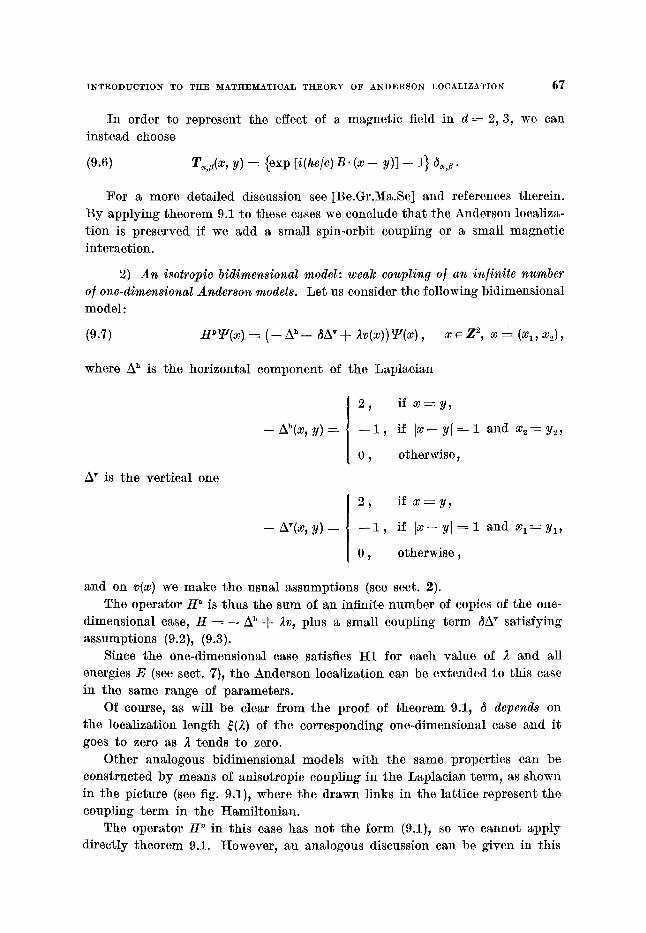
I N TRO D U CTI O N TO THE MATHEMATICAL THEORY OF ANDERSON LOCALIZATION 67

I n order to represent the effect of a magne t ic field in d : 2, 3, we can

ins tead choose

(9.6) T~,~(x, y) = {exp [i(he/c)B. (x-- y ) ] - 1} 8~,~.

For ~ more detai led discussion see [Be.Gr.Ma.Sc] and references therein. B y apply ing theorem 9.1 to these eases we conclude t h a t the Anderson localiza- t ion is preserved if we add a small spin-orbit coupling or a small magnet ic

interact ion.

2) A n isotropio bidimensional model: weak coupling o] an infinite number o] one-dimensional Anderson models. Let us consider the following bidimensional model :

(9.7) HPT(x) : ( - - A h - ~A'~- 2v(x))T(x) , x e Z 2, x : (xi,x2) ,

where A ~ is the hor izonta l componen t of the Lapl~cian

M is the ver t ica l one

- - Ah(X, y) ----

- A V ( x , y ) = -

2, if x : y ,

- - 1 , if I x - - y [ : 1 and x 2 ~ y 2 ,

0, otherwise,

2 , if x - - - y ,

- - 1 , if Ix - - Y l : 1 and x 1 - ~ - YI,

0 , o therwise ,

and on v(x) we m a k e the usual assumpt ions (see sect. 2). The opera to r H ~ is thus the sum of an infinite n u m b e r of copies of the one-

dimensional case, H : - - A h ~ ~v, plus a small coupling t e r m 8A v sat isfying

assumpt ions (9.2), (9.3). Since the one-dimensional case satisfies H1 for each value of 2 and all

energies E (see sect. 7), the Anderson localization can be extended to this case in the same range of paramete rs .

Of course, as will be clear f rom the proof of theorem 9.1, 6 depends on the localization length ~(2) of the corresponding one-dimensional case and it goes to zero as ~ tends to zero.

Other analogous bidimensional models wi th the same proper t ies can be constructed b y means of anisotropic coupling in the Laplac ian term~ as shown in the p ic ture (see fig. 9.1), where the drawn links in the la t t ice represent the coupling t e r m in the Hami l ton ian .

The opera to r H p in this ease has no t the fo rm (9.1), so we cannot app ly direct ly theorem 9.1. However , an analogous discussion can be given in this

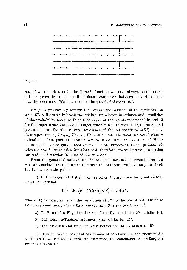
~ F. MARTINELLI a n d :E. SCOPPOLA

. . . . . . . . C-:----L /

�9 �9 m �9 �9 m �9 �9 m �9

I I I

I I

]Pig. 9. I.

case if we r e m s r k t h a t in the Green's funct ion we have always small contri- but ions given by the (( one-dimensional coupling >) between s ver t ical link and the nex t one. We now tu rn ~o the proof of theorem 9.1.

lProo]. A pre l iminary r e m a r k is ill order: the presence of the pe r tu rba t ion t e r m ~HI will general ly b reak the original t rans la t ion invariunce and ergodicity of the p robabi l i ty measure P, so t h a t m a n y of the results ment ioned in sect. 3 for the imper tu rbed case are no longer t rue for H p. In par t icular , in the genersl pe r tu rbed case the a lmost sure invar iance of the set spec t rum a (H p) and of

its components apo(HP), a~r adi~(H ~) will be lost. However , we can obviously extend the first p a r t of theorem 3.2 to s ta te t h a t the spec t rum of H p is contained in a 6-neighbourhood of a(H). More impor t an t all the probabilistic estimates will be translation invariant and, therefore, we will p rove localization

for each configuration in a set of measure one. F r o m the general discussion on the Anderson localization given in sect. 4 - 6

we c~n conclude tha t , in order to prove the theorem, we h~ve only to check the following main points.

1) I f the potentia.l dis t r ibut ion satisfies A] , A2, then for ~ sufficient]y small H ~ satisfies

where H~ denotes, as usual, the restr ict ion of H ~ to the box A with Dirichlet b o u n d s r y conditions, E is ~ fixed energy and C is independent of A.

2) I f H satisfies H1, then for ~ sufficiently small also H" sstisfies H1.

3) The Combes-Thomas a rgumen t still works for H ~.

4) The Frohlich and Spencer construct ion c~n be extended to H ' .

1) I t is an easy check tha t the proofs of corollary 3.1 and theorem 3.5 still hold if we replace H with H~; therefore, the conclusion of corollary 3.1 extends also to H ~.

INTRODUCTION TO THE MATHEMATICAL THEOI~Y OF ANDERSON LOCALIZATION 69

2) In order to verify the second point, we use the first resolvent ident i ty for H ~. If we denote by

we have

(9.8)

a~ v; x, y) ~ (H~ -- E)-~(x, y) ,

h e ( E , v) = G(E , v) - - G(E , v) ,~H~G~ v) .

(9.9)

The same holds for G~A(E, v) ~- (H~-- E) -1. For every E e I , a , 1 and 7 we can write

P{v; ~ IG~(E, v; x, Y)] < a~ with dist (x, ~A) > / / 4 } > yeOA

> P { { v ; X lion( E, v; x, Y)]-4- [(GA(E, v)(~H1GPA(E, v))(x, Y)I] < a ve~A

w i t h d i s t (x, 8A) > 1/4} n (v; IliA(E, V)[[ < r} f3 {V; l[G~l(J~, v)l [ < ~}} >

> P{v; ~. IGd(E, v; x, y) < a - - r2,~18Al with dist @, S A ) > 1/4}-- yeOA

- - P{v; IIGA(E, v)i 1 > ~'} - - P{v; IIG~A(E, v)l I > ~} .

The probabilities P(v; t](TA(E, V)H > ~} and P(v; I1G~(E, v)l I > ~} can be est imated by means of corollary 3.1; we have in fact

P(v; IIGA(E, v)t I > ~) = P{v; dist (a(HA(V)) , E) < 1]~}< CIA[? -~' .

Thus from (9.9) we conclude

(9.10) veSA

> P{v; 2 [O,t(E, v; x, y)[ < a with dist (x, 8A) > 1/4}-- 2ClA[? -~ , veSA

where a---- a - - ?~ 818A I. Suppose now tha t H satisfies B1 a t E. Then, using the basic Frohheh and

Spencer estimates in the form of theorem 4.1, it is easy to check tha t for all a < 1 and 1 large enough

(9.7) p{v; ~: EeA(~,v;x,v)l<~ for Ix-vl>~/4}<~(a,~,~)/2. vEOA

Therefore, if 1 is large enough and if we chose (~ = ~(1) so small t ha t % > a > 0 and ~, such tha t 2C[A[? -~' < s(d, l, a)/2, then using (9.7) the r.h.s. of (9.6) is bounded from below by

1 - s(a, ~, a) /2 - 2 C l A I r - ~ > 1 - - s(a, ~, a ) .

70 F. MARTINELLI a n d E. SCOPPOLA

3) The Combes-Thomas a rgumen t (see sect. 2) still holds in the pe r tu rbed case .

The proof here is exac t ly the same as in the imper tu rbed case (see sect. 2).

4) Final ly Frohlich and Spencer 's construct ion can easily extended to H" with small changes if one observes t h a t the coupling opera tor be tween two regions separa ted b y a bounda ry ~, which in the imper tu rbed case was represented b y

1 , if { x , y } e O ,

F(x, y) = O, o therwise ,

reads now

where

/-~ = P § 3 F ' ,

- - ~ I ( X , y ) , i f {x, y} e ~ ,

["(x, y) ---- 0 , otherwise .

Remark. The hypotheses (9.2), (9.3) are not the more general ones and they can be cer ta inly be weakened. For instance, assumpt ion (9.3) can be replaced b y a sufficiently fas t fall off of H~(x, y) when Ix-- y[ is large (e.g., exponential) . Wi th li t t le ex t ra work also assumpt ion (9.2) can be re laxed; we ment ion, for instanc% the case of H~ stochast ic and IIH~II large with small probabi l i ty .

10. - The cont inuous random Schr6dinger equation.

We explain in this section how to ex tend our results to the t rue Schr6dinger equat ion in the cont inuum R ~. In this case there exists no direct well-defined

analogue of the Mlderson model and one has to choose among different proposals for the r andom potent ial . The simplest case would be t h a t of a potent ia l equal to a r andom cons tant h i on each unit cube C~ centred a t the site i of the lattice Z d. This was ac tual ly the model considered by H o L ] ) ~ and 5IA~TI- NELLI [Ho.Ma] and has the technical advan tage t h a t some of the discrete s t ruc ture of the lat t ice Z a is preserved. I t was successively generalized b y MARTINELLI and SCO~POLA [Ma.Sc] in order to include potent ia ls t h a t are equal to h~0 o on each cube C~, where ~0 is a fixed posi t ive funct ion whose shape is t ha t of a smooth well. Al though the way in which one adap ts to the cont immus case %he techniques developed for the Anderson mode l m a y depend on the specific model, we believe t h a t the ideas behind our approach are sufficiently general to cover a large class of si tuations. Therefor% we will discuss

I N TRO D U CTI O N TO THE MATHEMATICAL T t IE ORY OF ANDERSON LOCALIZATION 71

a very concrete t ru ly continuous case which has appeared many t imes in the physical l i terature instead of t ry ing to work in great generality.

The model t ha t we choose is an ideahzation of a single part icle moving in a sea of impurities randomly distr ibuted in R d, each of them producing an

a t t rac t ive potent ia l whose s t rength depends on the impur i ty . More precisely let {xi} be a realization of a Poisson random field Po on R a

of density 5, namely

(10.1)

i) P o { # ( w , e A) = n} = exp [ - elAlJ(elAI) ' /n! , A c R ~,

ii) the distr ibution of the points x~ in A condit ioned to the event t ha t their number is n is the n-th power of the uniform distri- but ion on A.

Let also {q~} be a sequence of i.i.d, r andom variables with values in [0, 1] and common distr ibution Pl(dq) = / ( q ) dq, where we assume ]]l~ < ~ . We set

t9 = [0, 1] N • (Ra) N and P = Po x P~.

Final ly let V o :Rd-+ R be a continuous funct ion such tha t

(lO.2)

a) Vo(x)<O,

b) [Vol~< c~,

c) Vo(x) = O , Ixl > i.

Then we take as a random potent ia l V(x) the funct ion

(10.3) V(x) = ~ q~ V o ( x - x~).

Using (10.1) i t is easily seen [Ki.Ma.1] t h a t the SchrSdinger operator

(10.4) /~ = -- A + v

is a solf-adjoint operator on L2(Rd). I t is also easy to check tha t the family of shifts {T, x Tv} defined on /2 by

(lO.5) {T, • T,}{(q,), (x,)} = {(q,+), (x, + y)}

acts ergodically on (~2, P).

By the same arguments given in sect. 3 this fact is sufficient to ensure t h a t the spectrum of H is almost surely constant . Moreover~ since with posit ive

72 r. 3IARTINELLI and E. SCOPPOLA

probabi l i ty we can find a box of a rb i t ra r i ly large size complete ly e m p t y of impurit ies, the spec t rum of H will contain the spec t rum of the free Laplacian (kinetic energy), namely the posi t ive half-line [0, pc). On the other hand, the funct ion V o being negat ive, a region with a ve ry high densi ty of impuri t ies will substain s ta tes of arbi t rar i ly negat ive energy. Thus the spec t rum of H will contain arb i t rar i ly negat ive energies.

Our a im is to show tha t for low impur i t y densi ty Q the states of negat ive energy are exponent ia l ly localized in space. For concreteness let us fix E o > 0

and let us invest igate the propert ies of s ta tes with energy in (-- o ~ , - ~o). The main idea is the one a l ready explained in sect. 4. We first find a subset

S o of R d on which the s ta tes mus t be localized and then we show tha t wi th probabi l i ty one the configuration {x~} of the impuri t ies and the values of thei r

coupling constants {q~} are such t ha t the tunnel l ing among the clusters of S o does not t ake place over too large distances. In order to simplify all ~,he geometr ic construct ions which are necessary for the proof of this result (see

sect. 5, 6), it is convenient to ((discretize ,> the space R a by introducing the ; ) covering of R a with the cubes ~C~, of side uni ty , centred a t the sites of Z d and

with sides paral lel to the co-ordinNe axes. Then we define S o as follows:

(I0.6) ~s'o = U Ui , iego

w h e r e

do.7) So = {J e Za; V(x) = 0 for some x e C~.}.

In general, if X c Z a, then A c R a will denote the set

(!o.s) A = U C~. J~2

I t should be noticed tha t , since the funct ion V 0 has (~ range ~> equM to one, the events {1 CSo} and {i e ~qo} are independent only if [ i - - J l > ~/d" This fact , however, will affect in a negligible way the probabil ist ie est imates . We now r e m a r k tha t , if o<< 1, then

(lo.9) e{j e &} < P{#(im~uriti,,s in U c,) > o) = o(,,)<< 1. b - J l < ~

Fur the rmore , i t is also clear t h a t ally s ta te of energy E Iess t han or equal

to - - E o m u s t be e x p o n e n t i a l l y local i zed on S o with (( mass )) of order ~ / ~ , since the complement of S o is a t rue poten t ia l barr ier for E of height [E[. Thus the set Go, and, therefore, So, enjoys the same propert ies of the set S o defined in sect. 4 for the Anderson model. In order to analyse the tunnell ing among the dus te r s of So, one adap ts to the continuous case the multiscMe pe r tu rba t ive scheme of Frohlich and Spencer (see sect. 5). All the geometr ical construct ions

INTRODUCTION TO THE MATHEMATICAL THEORY OF ANDERSON LOCALIZATION 7~

are first done on the la t t ice Z ~ and then t ransfered back to the R e using (10.8).

The only i m p o r t a n t new technical p rob lem is due to the fac t t ha t for the SchrSdinger equat ion there exists no direct analogue of the bounda ry opera tor -P~A defined in sect. 2 connect ing the interior wi th the exter ior of a region A, and~ therefore, the resolvent equat ion (2.14) which represented a ma in tool

in the pe r tu rba t ion expansion mus t be modified. The solution to this p rob lem is, of course, suggested na tu ra l ly b y the s tandard Green's formula. I f A is a bounded closed connected domain of R e and A, B are such t h a t A ~ A u B,

then for x e A and y e a

(10.10) GA(E 4- ie; x, y) -~

-= GA(E 4- ie; x, y) + fdz(~.,a ~(E 4- ie; x, z))G ~(E 4- ie; z, y) , ~ A c) c~B

where ~,~ denotes the no rma l der iva t ive a t the poin t z. Thus in the continuous case one has to control not only the Green's funct ion

bu t also its no rmal derivat ive. However , as should be expected, the la t te r is bounded b y the first one if dist (x, ~A n c~B) > 0.

Zemma 10.1 [Ho.Ma]. Le t A be a finite union of cubes C~. Then there exists a constant k independent of e, E and A such t h a t for any x e A with

dist (x, ~A) > i and any z ~ ~A one has

]~,G A(E @ ie; x, z) I < k[G A(E 4- i~; x, z)].

I n this way in [Ho.Ma] all the mate r ia l described in sect. 5 was t ransposed to the cont inuum.

I t remains to discuss the probabi]ist ie pa r t of the proof or be t t e r its funda- men ta l ingredient assumpt ion tt2. In general, i t is much more complicate to

ver i fy tI2 in the cont inuous case t h a n in the discrete case and the specific features of the model m a y help in a significant way (see, e.g., [Ma] ~or the same prob lem in the context of the wave equat ion in domains wi th r a n d o m boundaries). T h a t some new problems mus t arise it should be clear f rom the proof of corollary 3.1. There we used in a ve ry subs tant ia l way the fac t t h a t the

opera tor v o 6o(x ) was el r ank one and in our new contex t this p rope r ty is clearly l o s t . Al though i t is now possible to p rove H2 along the same lines of corol- la ry 3.1 (see [Ko.Si]), we prefer to give a r a the r direct prooi based on the old Wegner ' s idea (see also [Ho.Ma] and [Ma.Sc] for the same proof in simpler c a s e s ) .

Zemma 10.2. For any bounded set ~ c Z e and any E < - m

P(dist (E, ~(//A)) < ~) < c0nst" [/l~elAld/2+%.

74 r.. ~IARTINELLI and E. SCOPeOLA

Proo]. B y the Chebyshew inequal i ty

(10.11) P{dist (E, ~(HA)) < ~} < fdP((o)fdZ'(~/~E')YC(E', HA({Z}, {q})),

where N(E', HA({X~} , {qi})) = ~{eigenvalues of HA({Xi} , {qi}) less than E'}. Wegner 's idea is to Lranfer the ~/~E' derivat ive into a derivat ive with respect to the q~'s in order to make the dP(co) integrat ion more or less explicitly. For this it is enough to prove tha t for any 6 > 0 small enough

< N(E', Hz({x,}, {q, § c 6 } ) ) - N(E', Hz({xi}, {q~--c6}))

for a suitable constant v independent of 6, A. Assuming (10.12) we get tha t the r.h.s, of (10.11) is bounded by

(10.13) cfdeo( }f H de (q,)de (q,)fdE' Z ~/~q~5~( E', HA({Xi}' {q~})) <

#{x~e A} C ! E~IA[ d/2+2 .

The final est imate comes from the estimates

(lo.14)

(10.15)

~ ( E , H A({x~} , {qi : 1})) < eoust . IA 1 (E + @ (xi~ A')) a'z ,

5 nd/"+~P( # {x~ c A'} - n) < eonst, o l A f "~+'z ,

where A' is a neighbourhood of A of radius one. The first est imate comes f rom the fact tha t , if there are n impurities inside

A', then the potent ia l V in A is not more negat ive than -- const .n . I t remains to prove (10.12). Let En({Xi} , {q,}) be the n-th eigenvalue of HA({Xi}, {q~}) which we assume to be smaller than E ' ~ 6. Then by the min-max principle

we have

(10.16) E . ~ - sup inf <q,,--Aq~) § (~, V~v>.

{,~ ... ~ . - ~ }

Since E~ < E 'q - 6 < E § 6 § e and since -- A is a positive operator, the

functions ~ over which we take the infimum must be such tha t

(lo.17/ v >j = qifdxVo(X-- > r t- 6 --

Therefore, for such functions, we must have

(10.18) ~, 26/[E]fdxVo(x -- xgq~(x) 2 > 26([E]- 6 -- s)/[E[ > 6,

where we have used the assumption 0 < q~ < 1.


Thus by (10.16) En({x~} , {q, + 2alibi})< E' and the first half of (10.12) follows. The second half is proved in a similar way.

This concludes the proof of the lemma and also of the discussion of the continuous case.

11. - Other approaches to m u l t i d i m e n s i o n a l Anderson loca l i za t ion .

Independently of the work of Frohlich, Martinelli, Scoppola and Spencer, two other group of people, S~wo~ and WOLFF [Si.Wo] and DELY0~, LEVY and S0tr~LA~D [De.Le.Sou], provided two similar proofs of the Anderson localization at high disorder or low energy completely different from the one presented in the previous sections. These approaehs are rooted into three different works:

i) The Frohlich and Spencer exponential bounds on the Green's function ( H - J ~ - ie)-l(O, x) as Ixl ---> c~ for a fixed energy E (see theorem 4.1).

if) Our proof of the absence of absolutely continuous spectrum for low energies or high disorder [Ma.Se]. This paper in particular pointed out

a) the strong connection between the spectral properties of the operator H and the bounds on the Green's function proved in [Fr.Spl];

b) the crucial role played in a rigorous analysis of localization by the generalized eigenvalues and eigenftmetions of H(v).

iii) The so-called Kotani's trick [Ko2], which, assuming an absolutely continuous potential distribution, allows one to derive statements for almost all potential configurations v and almost all energies with respect to the spectral measure dp(v) of H(v) from statements which hold for almost all energies with respect to the Lebesgue measure and almost all potentials v.

Let us now state the main theorems of [Si.Wo] and [De.Lo.Sou], respectively,

Theorem 11.1 (Simon, Wolff). Consider the two statement for the d- dimensional Anderson model:

a) for a.e. v, H(v) has only point spectrum in (a, b);

b) for a.o. E ~ (a, b) and a.e. v

Then

Jim [ ~ ]G(E ~ is, v; n, 0)[ 2 ] < ~x~.

i) if dP is purely absolutely continuous (d.c.), b) implies a);

if) if d = 1 and dP has a nonzero d.c. component, then b) implies a);

~ F. ~IARTINELLI and E. SCOPPOI.A

iii) if the a.e. component of d P has essential suppor t (-- 0% ~ ) (e.g., d P Gaussian), then a) implies b).

Theorem 11.2 (Delyon, Levy, Souillard). I f the following hypotheses are

verified:

h l : there exists a posit ive constant a and posit ive valued functions C(e) on R+ and c~(E) on I c R such tha t for a.e. E c I , with respect to the Lebcsgue measure, for any finite box A c Z J, ~, ~ Z ~, and e > 0 one can find Y2(A, ~, E, e)

with P(f2(A, n, E, ~)) > 1 - - e such tha t if v c D(A, n, E, e) for all m ~ A

l a A E , v; ~, m)l < C(~) .exp [ - - ~(K). Im -- ~1] ;

h2 : the potent ia l a t the sites of the (~ slice ~> Z ~ lx[0~ 1] have independent

distr ibutions with bounded densities with respect to the Lebesgue measure.

Then with probabi l i ty one the spec t rum of H in I is pure point and non- degenerate and all the corrispondiug eigenvectors are exponent ia l ly decaying

at infinity. The hypotheses b) of theorem 11.1 and h l of theorem 11.2 are verified~

for high disorder or low energy, by means of the Frohlieh ~nd Spencer result

on the decay of the Green's functions. The interest ing idea behind this different approach is t ha t the singulnr

continuous spec t rum is too uns table to be present in the Anderson model. In order to unders tand the exact meaning of this instabil i ty, we want to recall the different bu t re la ted one-dimensional model with a lmost periodic potent ia l

given by

v(y~) = ,~ cos :~(On 4- x)

with 0 irrat ional, x e [0, 1], ~ ~ Z, known as a lmost Mathieu equation. For such a model m a n y results are known (see for a review [Si6]~ [Av.Si]) and in par t icular it is p roved tha t for ~ > 2 the L y a p m l o v exponent (see (7.15)) is

posi t ive for all energies, so tha t there is no absolutely continuous spectrum. 3[oreover, for par t icular choices of 0 s-cry near to ra t ional numbers we

can apply to this ease the general result of Gordon [Go] which excludes the presence of localized states for potent ia ls very close to the periodic ones. Thus for this par t icular choice of 0 and for 2 > 2 we can conclude by exclusion t ha t

the spee t rmn is singular continuous. This str ieking result points ou~ tha t the posi t iv i ty of the L y a p u n o v ex-

ponent is not sufficient to have localized states. La te r on KOTA>'I [Ko2] (see also [Ca3]) proved t h a t this kind of spec t rum

is ex t remely unstable : if a smM1 r andom pe r tu rba t ion with an absolutely con- t inuous dis tr ibut ion is added at two nearest -neighbours sites, then the singular

spec t rum disappears turning into pure point spectrum.

INTRODUCTION TO THE MATHEMATICAL THEOICY OF ANDERSON LOCALIZATION ~ 7

The same argument can be applied to the Anderson model for ,t large where the posi t ivi ty of the Lyapunov exponent is replaced in the mult idimensional case by the exponential decay of the Green's functions. In these approaches it is not necessary to estimate, as we did, finite-volume Green's functions with energies chosen among the generalized eigenvalues of H. Once the decay of the Green's funct ion is known with probabi l i ty one for a lmost all energies with respect to the Lebesgue measure, then, by means of Kotani ' s trick, this p roper ty is t ransfered into a s ta tement for almost all potent ia l configurations and all the generalized eigenvalues.

This procedure has the advantage of being shorter than the one described in this paper. However, in avoiding a detailed analysis of the potent ia l configurations, the resulting information about the structl~re of the eigenfunctions is restr icted only to their behaviour at infinity and the whole physical mechanism leading to localization is not as t ransparent as we believe it is in the approach presented in this paper. I t was not possible, for example, to derive by this method the results of corollaries 4.2, 4.3. Fur thermore , the absolute cont inui ty of the potent ia l distr ibution dP(v), which plays an essential role in Kotani ' s work, precludes the application of the above theorems to interesting models with singular measures like the b inary alloy described in sect. 7.

Besults on Anderson localization similar to those reviewed in the present section were announced by GOLDSttADE, bu t the paper is not available, as yet .

We would like to warmly thank G. JOg~A-LASIbTIO for his strong encourage- ments to write this work, for his contr ibutions and for his construct ive criticism.

A P P E N D I X A

Proo/ o/ theorem 3.1.

a) For shortness and simplicity we will prove only the first assertion. The proof of the other two uses exac t ly the same kind of ideas bu t requires an addit ional subtle discussion of the measurabi l i ty of some operator-valued funct ion which we prefer to skip. The interested reader is referred to [Xi.Ma]].

Let , for any real ~ ~nd #, P~,~(H(v)) be the spectral projection of H(v) a, sso- ciated with the in terval ()L, #] and let/~, ,(v) be the dimension of its range. Using Stone's formula [Re.Si] i t follo~=s immedia te ly tha t /~,~ is a measurable func- t ion on s Fur thermore , since H(v) and H(Y~v), x E Z d, are unitari ly equivalent (see sect, 2), /~.,~ is lef t invar iant b y the shifts {T~}~z~ ~nd, therefore, by the ergodic theorem, there exists a set ~0 e ~ with #(~20) = ] such that /a .~ is constant over ~o for all rat ionals ,~ and /~. ~ o w it is well known tha t E E a ( H ( v ) } if and only if / a ,~>0 , , ~ , # e 0 , 4 < E < # . Using the above discussion, we get immedia te ly tha t a(H(v)) = a(H(v')), v =A v', v, v' e ~o.

7 8 F. M A R T I N E L L I and E. SCOPPOLA

This proves the first s~atement.

b) I t is proven in [Pal l , [Ki .Mal] t ha t ]~,# is almost surely ei ther zero or infinity. Therefore, if E ~ X, then almost surely ]~,~,(v) = - ~ if 2, # ~Q with 2, < E < ,a. This implies tha t E ~ aa~(H(v)) ahnost surely. By repeating the above argument for all rat ionals in X and by a l imiting argument we get the result.

Proo] of theorem 3.2. We ha~e only to show tha t

[o, 4(1] @ XoC X

(for the opposite inclusion see sect. 3). Let % e X 0 b e fixed and let ~ > 0 . For any k e [ 0 , ; ~ ) a l e t

exp [ik o,~3/fALI "'~, x e A ~ , (A. 1 ) ~(.r) = 0, otherwise .

Since (--Aq~.)(x) = ( 2 d - - 2 ~ cos_k~)7~k,x), it follows by explicit computat ion i = l , . . . , d

tha t , for all v ~ ~ with

(A.Z) Jr(x) - - ~'oI < ~, x c A~ ,

(A.3) %/ i'~AL]/]AL] . ( \ i / )

The above est imate shows tha t for such configurations

(~.4) dist (~("(v) , 2 d - - 2 ~ cos k~-~ % ) ) < ~ @ ~X/I@ALII[ALI. i

Since the probabi l i ty of the event described in (A.2) is positive for any ~ and L, we get, using (A.4) and theorem 3.1, tha t

"2d --"2 ~, cosk~ + roZ Z i

almost sure ly .

This in turn implies tha t Z'o + [0, 4d] c 2,', since k and Vo were arbi t rary.

Proo] o] the eriste~wc el the in~:,gr~ted de,~sity el states. We want to show the existence of the following l imit:

N(E) = l i ra I,ILI-IN(HA~, E ) .

Let us consider the p~rt i t ion of the box AL into subcubes C~ of side 21 and centred at the sites of the latt ice Z d ( 1 ) - =:(/d-~.)Z d (we ,~re implici t ly assuming tha t L - - ( ' _ ' ~ - L I ) I @ 2 ~ for some ~ t~N) . Thus the cubes C~ are separated by a latt ice line. If we restr ict the matr ix H ~ to 12(U~ C~), then the eigenvalues increase because of the mini-nmx principle and we have

y E) = y. N(H~,, E) . N(HA~, E) > ~ (H~c,,

INTRODUCTION TO TYDz, MATHEMATICAL THEORY 01~ ANDERSON LOCALIZATION 7 9

Therefore, iV(HAL, E) is a superaddit ive ergodic process and b y the mnlti- dimensional version of the superaddit ive ergodic theorem [Ac.Kr]

(A.5) l im 2Y(.[J[AL , E)/IA~, I = Sup E[N(HA, E)J/IA I L--* + oo A c Z a

almost surely. Analogously, one proceeds with the Xeumalm boundary conditions. In

this ease, the inser t ion o f /~eumann conditions inside A lowers the eigenvalues and, therefore, IV(HA, E) becomes subuddit ive in A and one gets

(A.6) lira iV(Ha=, E)/]Az[ : inf E{iV(HA, E)}/IALI. + o o A cZa

A P P E N D I X B

We discuss here the main points for a renormalized version of our proof of localization which enables us to extend the localization result to cases verifying the general assumptions H1, H2 instead of A1, A2 and 2 large. Assumptions t t l and H2 can cover in fact a larger class of system and we can conjecture tha t t hey are not too far f rom being necessary and sufficient conditions for localiza- t ion in random systems.

H I , I t2 were essential not only to analyse the one-dimensional case for each energy and each 2, as shown in sect. 7, bu t also in the proof of the absence of ve ry slow t ime evolut ion (see sect. 8).

The main pa t t e rn of the proof of localization as i l lustrated in sect. 4 for 2 large does not change; therefore, we outline here only the main technical points which have to be modified.

Le t Eo be such tha t H1 holds for Eo. As in sect. 4, we first proceed to ident i fy a subset So of the latt ice Z ~ on which the states with energy ve ry close to Eo must be concentrated. The main requirements which have to be fulfilled by So are (see sect. 4):

a) So must consist of clusters of typical size much smaller than thei r typical mutua l distance.

b) On the complement of So the Green's funct ion Gz~\s~ x ,y ) must decay exponent ia l ly as Ix - - y] -+ c~ uniformly in E e [Eo-- 8, Eo + 5] for 6 small enough.

Sn order to construct So in ~ simple way, i t is convenient to introduce the new lat t ice

( B . 1 ) gd(1) = l Z ~ , Z e N ,

and to associate to each site j of Zd(1) the cube B~ in Z a centred at j of side 21. ~or nota t ion convenience we will denote by A~ a subset of Za(l) (R ~-rescaled), corresponding to the subset A of Z ~ with

(B.2) A = [..J B~. JeA~

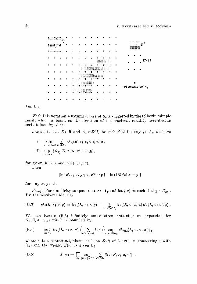
8 0 F. M A R T I N E L L I and :E. SCOPPOLA

)!}!!!!!!i!i!8. . . . . . . . . . . . J

:::::::1 )!

: : : : : : : : : : : : : : : : : : : : : : : : : : : : : : :

: : : : : : : : : : : : : : : : : : : : : : : : :

i i i ! i i i i i i z z

Z2CL)

e l e m e n t s of A R

Fig. B.2.

With this nota t ion a na tu ra l choice of So is suggested by the following simple resul t which is based on the i te ra t ion of the resolvent iden t i ty described in sect. 6 (see fig. 5.3).

Lcmma ~. Let E ~ R and ARcZa( / ) be such tha t for any j e A ~ we have

i) sup ~ pGB,(E, v; u, u')l < a , ]u-j]<ll2 u'eeB~

ii) sup " ii GBj(E, v ; u, u')[] < K ,

for given K > 0 and a ~ (0, 1/2d). Then

[(;~(E, ~,; x, .~t)l < K ~ exp [-- l n ( U 2 da)]x - y[]

for ally ,r~ y ~ A .

ProoJ. For s implici ty suppose t ha t .r e An and let j(y) be such t h a t y ~ B~(~). By the resolvent ident i ty

(B.3) G A ( E , ~ ; . r , y ) ~ G B : ( E , ~'; ,r, if) _L ~ GB:(E, v; x , u)GA(E, v; u', y) . (u,u')e~B~

We can i te ra te (B.3) infinitely m a n y often obtaining an expansion for GA(E, v; x, y) which is bounded by

(B.4) sup IGor(E, r; x, u)r ( ~ F(co)) sup [OB,,~,(E, v; u, u')[, u~Bz (o :x-->j(y) u, u' eBj(~)

where oJ is a nearest-neighbom" pa th oll Zd(/) of length /o~l connecting x with j(y) and the weight F((,)) is given by

(B.5) F(~,) = [I sup ~, ra , , (E, ~:; u, ~')l . i~(9 [u-il<l[2 u'e~B~


Using i) we get

(B.6) F(w) < alOl,

which, together with ii) and (B.4), gives the result. We have used the stand- ard fact that #(~o: i - + ] , Iwl----n} < (2d) ~ on the d-dimensional lattice.

Using the 1emma, it is now easy to construct a set So with the required properties a) and b). We define So by means of its rescaled part S0~, where

and

Zd\SoR= {ieZd(~); SUp ]~ ]~,(E,v; u,u')]< a [u--.t[ <~/2 u'eSB.*

dist (Eo, a(H,,)) > 1-(~+d/~)},

where ~ �9 (0, 1] and a �9 (0, 1/2d) are the constants appearing, respectively, in H2, H1.

We observe that, if, e.g., I E - Eel < exp [--1], then for any j �9 SoR

(B.7) SUp ~ IG~,(E, v; u, u')] < a + exp [-- 1C], [u--i]<l/2 u'~82~t

C �9 (0, 1), and

]I~,(E, v; u, u')[ I < 2.1 l+d/a .

Therefore, on the complement of So the Green's function decays exponentially uniformly for [E - - Eel < exp [-- 1].

Furthermore,

(B.S) P(j �9 So~)< P(dist (E0, a(H, , (v) ) )< /-(l+a/~)) +

+ P(3u; I ~ - i l < t/2, Z u" ~SBj

[Gr,(E0, v; u, u')[ > a)

and, therefore, by assumptions ~1, 1=[2 and corollary 3.1 the sites of SoR as l -+ co are very unlikely exactly as the sites of the set So constructed in sect. 4. This ensures that also requirement a) is satisfied. [[hus in this construction the role played by the coupling constant ~ in sect. 4 is played by the scale 1 which must be taken large enough (but finite) so that the probability appearing in (B.8) is sufficiently small. Typically 1 has to be much larger than the localization length at Eo.

We can now proceed to the construction of the sets san which are singular on the k-th scale and then to the proof of the exponential decay of the Green's functions by extending naturally definitions and results of sect. 3 to the problem on the lattice Zd(1).

APPENDIX C

In this appendix we give some of the mathematical details which were omitted in sect. 7 about the one-dimensional case. We start by stating without

82 F. MARTINELLI and :E. 8COPPOLA

proof Osseledec's theorem [Os] which is at the basis of the result of proposition 1.

Theorem. Let ~,,~ n c N, be a sequence of matrices of SL2,c such tha t

i) lim,n -~log(I ~ $1 ) 7 > 0 ii) lira , , - l log(]~Sn,) = O.

Then there exists a nonzero vector x such tha t

lira .n -1 log ([,'S ..... ~lX[[) = - - 7

and for any vector y not proport ional to x_

l i m n - 1 l o g ( I s ..... S~YH) = 7 .

Let now SE(X) be the random matrices introduced in sect. 7 and let FE(x) be the solution of the Schr6dinger equation (7.1) with initial condition q g , - - ! ) ---- 0, ~E',0) -- I. Using Furs temberg result, the matrices S g x ) satisfy the hypotheses of Osseledec's theorem with probabil i ty one and we get

Corollary. For any E e C there exists a set $Z~c ~ of #-measure one such tha t

lira (2L) -~ l o o ' ( l c g L + 1) ~ + 9~gL)~]) = 7(E),

where v(E) is the Lyapunov exponent at energy E.

Proo]. The result follows from theorem 1 and the above theorem if we can prove that with probabi l i ty one the vector (1, 0) ----r is not proport ional to the contract ing direction x_(E, c) given by Osseledec's result. This is clearly the case since, if x(E, v)----(1,0) with positive probabil i ty, then, by repeating tile whole ,~rgument to the left of the site x = - 1, we could construct with positive probabil i ty a solution Vgx) of eq. (7.1) which decays exponentially fast a.t plus and minus infinity. This in turn would imply tha t E is an eigenwdue of finite multiplici ty of H(r) with positive probabil i ty in con- t radict ion to the result of theorem 2 of sect. 3.

I t is not difficult to see ~Is] tha t the asymptoties of ~E(L - / 1) is the same to tha t of qw(L); this fact together with the above corollary proves proposi- t ion 1 of sect. 7.

We are left with the proof of theorem 2. We will use the notations of sect. 7. By (7.8) and proposition I we have that

(c.1) lira P{IGEO,L~(E, O, L) I < exp [-- (T(E) - s)L]} = 1 .

Using now the resolvent equation (see sect. 2) we can express GA(E, 0,/+) in terms of GEO,LI(E , O, L) as

(C.~) (]A(E, O, i+) = ~[O,LI~E, O, L){1-~- ~A(E, O, - - l )} .

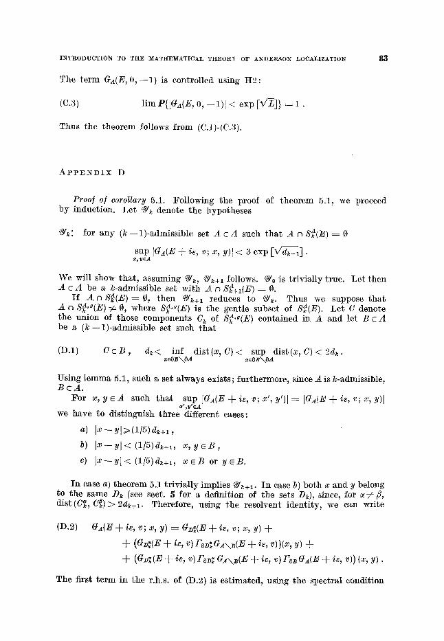
INTRODUCTION TO THE MATHEMATICAL THEORY OF ANDERSON LOCALIZATION

The term GA(E, O,--1) is controlled using II2:

(C.3) limP{[~A(E, 0,--1)] < exp IV/L]} ~--1.

Thus the theorem follows from (C.1)-(C.3).

83

APPENDIX D

Proo] o/ corollary 5.1. Following the proof of theorem 5.1, we proceed by induction. Let ~/~ denote the hypotheses

~/k : for any (k--1)-admissible set A c A such that A ~ S~(E)-~ 0

sup I ~ ( E + ~, ~; ~, ~)[< ~ e~p [Vd~__x].

We will show that, assuming ~k, ~ / k + l follows. ~0 is trivially true. Let then A c A be a k-admissible set with A n Sg+I(E)-~ O.

i f A ca SA(E)-~ O, then ~ + 1 reduces to ~/k. Thus we suppose that A g A ca S k, (E) r 0, where SA,g(E~ is the gentle subset of SA(E). Let C denote

the union of those components C~ of SA.~(E) contained in A and let B c A be a (k--1)~admissible set such that

(I).1) C c B , d~< inf dist(x, C)< sup dist(x, C)< 2dk. xeSB\OA ~eOB\~A

Using lemma 5.1, such a set always exists; furthermore, since A is/c-admissible, B c A .

For x, y e A such that sup IGa(E+ie, v ; x ' , y ' ) [~ [G~(E+ie , v ;x ,y ) ] ~t~feA

we have to distinguish three different cases:

a) [x--y]>(1/5)dk+l ,

b) [ x ~ y [ < (1/5) de+1, x, y e B ,

c) [ x ~ y ] < (1/5)dk+1, x r or y r

In case a) theorem 5.1 trivially implies ~/k+l. In case b) both x and y belong to the same D~ (see sect. 5 for a definition of the sets Dk), since, for ~ea fi, dist(C~, C~)> 2dk+l. Therefore, using the resolvent identity, we can write

(]).2) GA(E + ie, v; x, y) --- G1)~(E + ie, v; x, y) +

+ ((tD~(E + ie, v)F~D~G.4\B(E + i~, v))(x, y) +

+ (G~(E + i~, V)F~D~ G~\~(E + i~, v) F~G.4(E + i~, v)) (x, y).

The first term in the r.h.s, of (Z).2) is estimated, using the spectral condition

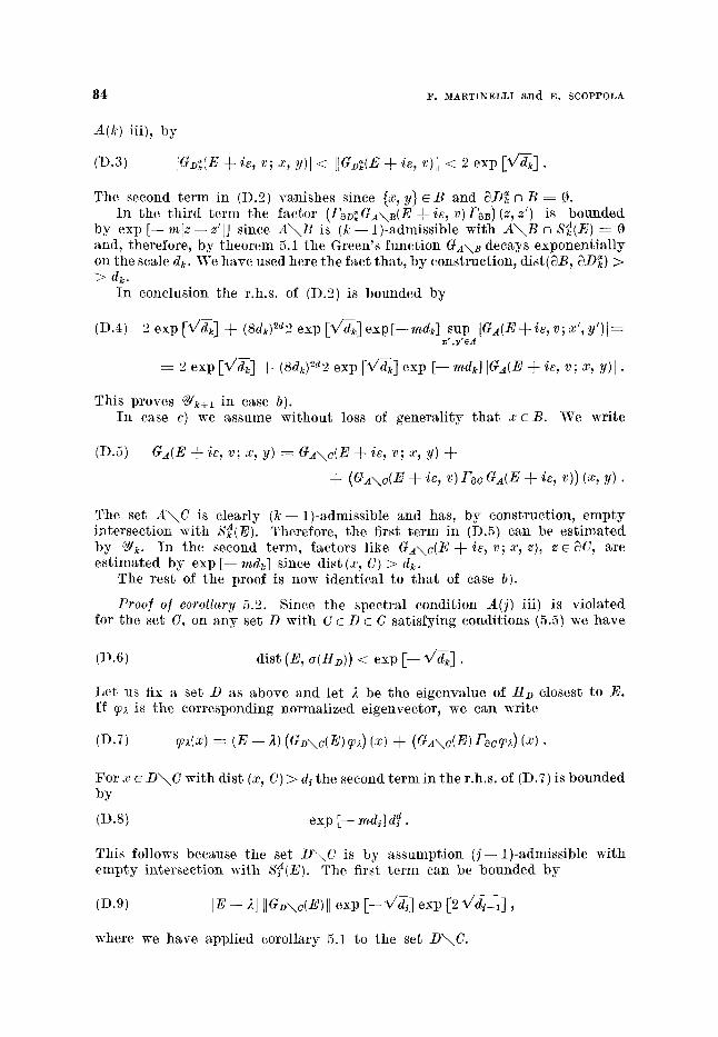
~4 F. MARTINELLI t~nd E. SCOPPOLA

A(k) iii), by

(]).~) Ir + i~, v ;.~, ~)l < I~ ~ ( E + i~, ~,)II < ~ exp [ V ~ ] .

The second te rm in (]).2) vanishes since {x, y} ~ B and ~ ~ ~ B = 0. In the th i rd te rm the factor (FeD~G~\~(E + i s , v)Fe~)(z,z') is bounded

by exp [-- mlz--z ' l] since A ~ B is (k - - 1)-admissible with A ~ B n SA(E) ~-- 0 and, therefore, by theorem 5.1 the Green's funct ion G~\~ decays exponent ia l ly on the scale d~. We have used here the fact tha t , b y construction, dist(~B, ~D~) >

dk. In conclusion the r.h.s, of (]).2) is bounded b y

(]).4) '2 exp [ V ~ ] ~- (Sdk) 2~ 2 exp [ V ~ ] exp [-- mdk] sup IG.4(E -~ is, v; x', Y')I= x',y'~A

--~ '2 exp I V y ] -~ (Sdk)2d2 exp [ V ~ ] exp [-- mdk] [G~(E ~- is, v; x, Y)I.

This proves ~/k+l in case b). In case c) we assume without loss of general i ty tha t x e B . We write

(]).5) GA(E -~ is, v; x, y) ~ G~\c (E -~ is, v; x, y) -~

§ ( G ~ \ d E § i~, v) F~c G.~(E § i~, v)) (x, y) .

The set A ~ C is clearly (k- -1) -admiss ib le and has, by construction, empty intersection with SA(E). Therefore, the first t e rm in (D.5) can be es t imated by ~/k. i n the second term, factors like GA\c(E ~-is, v; x, z), z E~C, are es t imated by exp [--md~] since dist (x, C ) ~ dk.

The rest of the proof is now identical to tha t of case b).

Proo] of corollary 5.2. Since the spectral condition A(j) iii) is violated for the set C, on any set D with C c D c C satisfying conditions (5.5) we huv6

(]).6) dist (E, a(Hz))) < exp [-- %/~] .

Let us fix a set / ) as above and let ), be the eigenvalue of H9 closest to E. If ~ is the corresponding normalized eigenvector~ we can write

(]).7) ~v~(x) : (E - - ~ ) ( G D \ c ( E ) ~ ) ( x ) ~- (GA\c(E)Fec~v~)(x).

For x ~ D ~ C with dist (x, C) ~ dj the second te rm in the r.h.s, of (]).7) is bounded by

(]).8) exp [-- mdj] d d .

This follows because the set D ~ C is by assumption ( j - -~)-admiss ible with empty intersect ion with SA(E). The first t e rm can be bounded b y

(]).9)

where we have applied corollary 5.1 to the set D~.C.

INTRODUCTION TO THE ~ATHEMATICAL THEORY OF ANDERSON LOCALIZATION

I n conclusion,

(~D.10) l~x(x) l < exp [ - V ~ I 2 ]

for all x e D \ C with dist (x, C) > dj. I f we now consider ~ as a funct ion on C .~ 3) b y set t ing it equal to zero

outside D, we see tha t , in C, ~ satisfies the equat ion

(O.11) (H - - A)~v~ : g~, ~ T ' s o = 0

wi th I[g~l[ < d~ exp [ - - V ~ / 2 ] b y (D.10). This implies

(Dn2) I[(Ho-- ;t)-~]l > 47 e~p [V'~/2],

t h a t is

(D.13) dist (E, a(Ha)) < [E - - ~1 § d7 exp [ - - V ~ / 2 ] < exp [-- d~/3].

Remark . To prove (D.]3) we have not used the fac t t ha t d iam C < 4d~.

I n par t i cu la r (D.]3) holds for any set A containing D. This fact was used in sect. 6 to derive (6.]8).

85

R E F E R E N C E S

[Ab.An.Li.Ra]

[Abou-Cha.An.Th]

[Ac.Kr]

[Al.Ho-Kr.Ki.Ma]

[An]

[Av.Si]

[Be.Gr.Ma.Sc]

[Ben.Pa]

a . ABRAHAMS, ~P. W. AND]~RSON, D . C . LICCIARDELLO a n d T . V . RAMAKRISHNAN: Scaling theory o] localization: absence o] quantum di]]usion in two dimensions, Phys. lCev. Lett., 42, 673 (1979). R. ABou-CHAcRA, P .W. ANDERSON and D.J . THOULESS: A sell- consistent theory o] localization, J. Phys. C, 6, 1734 (1973). ]V[. A. ACKOGLC and U. KR~NGEL: Ergodic theorems ]or superadditive processes, J. Reine Angew. Math., Band 323, 53 (1981). S. ALBEVERIO, R. HO~GH-KRo~N, W. KmSCH and F. MARTINELLI: The spectrum o] the three dimensional Kronig-Penney model with random point dejects, Adv. Appl. Math., 3, 435 (1982). P.W. ANDERSON: Absence o] di]]usion in certain random lattices, Phys. ]~ev., 109, 1492 (1958). J. AVRON and B. SIMON: Almost periodic SchrSdinger operators. I I : The integrated density o/ states, Duke Math. J., 50, 369 (1983); Transient and recurrent spectrum, J. Funct. Anal., 43, 1 (1981). J . BELLISSARD, D. R. GREMPEL, F. MARTINELLI a n d E. SCOPPOLA: Localization o/ electrons with spin-orbit or magnetic interactions in a two dimensional disordered crystal, to appear in Phys. Rev. Left., M.M. BENDERSKII and L.A. PASTUR: On the spectrum o/ the one dimensional SchrSdinger equation with a random potential, Math. USSE Sb., 11, 245 (1970).


[Ber]

[Bo]

[Bou.La]

[Bu.Kr.McK]

[C&m.K1]

[Call

[Ca2]

[Ca3]

[Ca.K1.Ma]

[Ch]

[Cha.Cha]

[Co.Fr.Sp]

[Cr.Si]

[De.Ku.Sou]

[De.Le.Sou]

[Day.Soul]

[Day.Sou2]

[Es. Sou]

[Ef]

[Fr.Ma.Sc.Sp]

J.M. BEREZANSKII: Expa~sion in eigen]unctions o] sel]-adjoint operators, Transl. Math. Monographs, 17 (American Mathematical Society, Providence, R . I . , 1968). R . E . BORLAND: The nature o] the electronic states in disordered one dimensional systems, Proc. R. Soc. London, Ser. A, 274, 529 (1963); see also B. 1. HALPERIN: Adv. Chem. Phys., 13, 123 (1967). P. BOUGEROLE and J. L.xCROIX: Products o] t~andom Matrices with Application to Schr6dinger Operator (Birkhiiuser, Boston, Mass., 1985). P. ]~. BULKA, B. KRAMER and A. MAcKINNON: Mobility edge in the three dimensional Anderson model, Z. Phys. B, 60, 13 (1985). J[. CAMPANINO and A. KLEIN: A supersymmetric trans]er matrix and diMere~tiability of the density o] states in the one dimensional Anderson model, Commun, Math. Phys., 104, 227 (1986). R. CARMONA: Exponential localization in one-dimensional disordered systems, Duke Mat]~. J . , 49, 191 (1982). R. CAR~IONA: Lectures on random Schr5dinger operators, in Proceed- ings Ecole d'Etd de Probabilitd, XIV (Saint Flour, 1984). R. CAR-~[ONA: Exponential localization in one dimensional disordered systems, Duke Math. J . , 49, 191 (1982). R. CAR~IONA, A. KLEIN and F. MARTINELLI: Anderson localization ]or Bernoulli and other singular potentials, to appear in Commun. Math. Phys. D. CHOWDHVRY : One parameter scaling theory o] localization, Comments Solid State Phys., 12, No. 2, 69 (1986). J. T. CHAYES and L. CHAYES: Proceedings o] the V I I I International Con]erence on Mathematical Physics, Marseille, 1986. F. CONSTANTINESCU, J. FROHLICIt ~nd T. SPENCER: Analyticity o] the density o] states and replica method ]or random SchrSdinger operators on a lattice, J. Stat. Phys., 34, 571 (1983). W. CRAIG and B. SBION: Log Holder continuity o] the integrated density of states lot stochastic Jacobi matrices, Commun. Math, Phys., 90, 207 (1983). F. DELYON, H. KUNZ and B. SOUILLARD: One.dimensional wave equation in disordered media, J. Phys. A , 16, 25 (1983). F. DELYON, Y. LEVY and B. SOUILLARD: Anderson localization ]or multi-dimensional systems at large disorder or low energy, Commun. Math. Phys., 100, 463 (1985); Approach h la Borland to multidimensional localizatiot~, Phys. Rev. Lett., 55, 618 (1985). P. DEVlLL.~RD and B. SOWLLA~D: Localization o] sur]ace waves ou a rough bottom, to appear in J. Fluid Mech. P. DEVILLARD and B. SOUILLARD : Polynomially decaying transmission ]or the nonlinear SchrSdinger equation in a random medium, J . Stat. Phys., 43, No. 3/4 {1986). D. ESCANDE and B. SOUILLARD: Localization o] waves in a ]luc- tuating plasma, Phys. Rev. Lett., 52, 1296 (1984). K . B . EFETOV: Supersymmetry method in localization theory, Soy. Phys. J E T P , 55, 514 (1982); Supersymmetry and the theory o] disordered metals, Adv. Phys., 32, 53 (1983). �9 J. FROHLICH, F. MARTINELLI, E. SCOPPOLA and T. SP]~NCER: Constructing proo] o/localization in the Anderson tight-binding model, Commun. Math. Phys., 101~ 21 (1985).

INTRODUCTION TO THE I~IATHEMATICAL THEORY OF ANDERSON LOCALIZATION ~7

[Fr.Spl]

[Fr.Sp2]

[Fr.~p3]

[Fr.Sp.Wa]

[Fu]

[Go.N[ol.Pa]

[Go] [Gra.Gre.J-L]

[Ha]

[He.Sj]

[Hi]

[Ho.Ma]

[Is]

[J-L.Ma.Scl]

[J-L.Ma.Sc2]

[J-L.Ma.Sc3]

J. :FROHLICH and T. SeENCEIr Absence o] di/]usion in the Anderson tiyht bindi~g model ]or large disorder ]or low energy, Commaen. Math. Phys., 88, 151 (1983). J . FROHLICIt and T. SPENCER: A rigorous approach to Anderson localization, Phys. Rep., 103, 9 (1984); Mathematical theory o] An- derson localization, in Proceedings o] the I .A .M.P. Con/erence at Boulder, August 1983, Physica (Utrecht) A, 124, 303 (1984). J. FROItLICIt and T. SPENCER: The Kosterlitz-Thouless transition in two-dimensional Abelian spin systems and the Coulomb gas, Commun. Math. Phys., 81, 527 (1981). J. FROI~LICH, T. SPENCER and C. E. WAY~E: Localization in disordered, nonlinear dynamical systems, J. Star. Phys., 42, 247 (1986). H. FUSTEMBERG: Noncommuting random products, Trans. Am. Math. Soc., 108, 377 (1963). YA. GOLtDSHEID, S. ~-~r and L. PASTUR: Pure point spectrum o] stochastic one dimensional SchrSdinger operators, Funet. Anal. Appl., 11, [ (1977). A. YA. GO~DON: Usp. Math. Nauk, 31, 257 (1976). S. GRAFFI, V. GRACCHI and G. JO~A-LAsI~IO: Tunneling instability via perturbation theory, J. Phys. A, 17, 2935 (1984). B. HALPERIN: Properties o/ a particle in a one dimensional random potential, Adv. Chem. Phys., 13, 123 (1967). B. HELFFEn and J. SJOSTRAND: Multiple wells in the semiclassical limit-l, Commun. Partial Di//er. Equ., 9(4), 337 (1984); Putts mul- tiples en limite semiclassique. I I : Interaction moldculaire-symmdtries- perturbation, Ann. Inst. Henri Poincard, 42, 127 (1985). S. ItIKAMI: 4-expansion /or Anderson localization in a strong spin. orbit coupling case, J. Phys. (Paris) Lett., 46, L719 (1985). H. HOLDEN and F. MARTINELLI: Absence o] di]]usion near the bottom o] the spectrum/or a SchrSdinger operator on L~(R~), Commun. Math. Phys., 93, 197 (1984). K. ISHII: Localization o/ eigenstates and trasport phenomena in the one-dimensional disordered systems, Prog. Theor. Phys. Suppl., $3, 77 (1973). G. JO~A-LAsINIO, F. MARTINELLI and E. SCOPPOLA: ~ew approach to the semiclassieal limit in quantum mechanics. I: Multiple tunneling in one dimension, Commun. Math. Phys., 80, 223 (1981). See also G. JO~A-LASINIO, F. MARTINELLI and E. ScoPPoL~: The semiclassieal limit o/ quantum mechanics: a qualitative theory via stochastic mechanics, Phys. Rep., 77, 313 (1981). G. JONA-L_asINIO, F. MARTIN]~r.LI and E. SCOreOLA: Multiple tunnelings in d-dimensions: a quantum particle in a hierarchical potential, Ann. Inst. Henri Poineard, 42, 73 (1985); Quantum partiele in a hierarchical potential with tunneling over arbitrarily large scales, J. Phys. A, 17, L635 (1984). G. JONA-LASlNIO, F. MARTIN:ELLI and E. SCOPPOLA: Tunneling in one dimension: general theory, instabilities, rules o] calculation, applications, in Mathematics q- Physics, Lectures on Recent Results, Vol. 2, edited by L. STREIT (World Scientific Publ., Singapore, 1986).


[Kam]

[Ki.Mal]

[Ki.Ma2]

[KI.Ma.Pe]

[Kol]

[Ko2]

[Ko.Si] [Ku.Soul]

[Ku.Sou2]

[La]

[Le.Ra]

[LP]

[Li]

ILl]

[Ma]

[Ma.Mi]

[Ma.Sc]

See, for instance, V. I. ARNOLD: Metodi matematici della meccanica classica, (Ed. Riuniti, Ed. Mir, Milano 1979); G. GALLAVOTTI: Mec- canica elementare (Boringhieri, Torino, 1980); see also Proceedings o] the 1984 Les Houches Summer School on Critical Phenomena .... edited by K. 0S'rERWALDER and R. STORA (1985). W. KIRSCH and F. ~-~ARTINELLI: On the ergodic properties o] the spectrum o/ general random operators, J. Reine Angew. Math., 334, 141 (1982); On the spectrum o] Schr5dinger operators with a random potential, Commun. Math. Phys., 85, 329 (1982). W. KIRSCH and F. MARTINELLI: On the density o] states o] Schrd- dinger operators with a random potential, J . Phys. A, 15, 2139 (1982); Large deviations and the Li]shitz singularity o] the integrated density of states o] random Hamiltonians, Commun. Math. Phys., 89, 27 (1983). n . KLEIN, F. MARTINELLI and F. PEREZ: A rigorous replica trick approach to Anderson localization in one dimension, Commun. Math. Phys., 106, 623 (1986). S. KOTANI: Lyapunov indices determine absolutely continuous spectra o/ stationary random one-dimensional SchrSdinger operators, Proc. Taniguchi Symposium S.A. Katata (1982). S. KOTANI: Lyapunoc exponents and spectra ]or one.dimensional random SchrSdinger operators, to appear in Proceedings of the 1984 American Mathematical Society, Con]erence on Random Matrices and their Applications. S. KOTANI and B. SI)ION: private communication. H. KUNZ and B. SOUILLARD: Sur le spectre des opdrateurs aux di]- ]drences ]inies aldatoires, Commun. Math. Phys., 78, 201 (1980). H. KuNz and B. SOUILLARD: The localization transition on the Bethe lattice, J . Phys. (Paris) Lett., 44, L411 {1983). J. LACROIX: Singularitd du spectre de l'opdrateur de SchrSdinger aldatoire dans un ruban ou un demi-ruban, Ann. Inst. Henri Poin- car~ A, 38, 385 (1983); Localization pour l'op~rateur de SchrSdinger aldatoire dans nn ruban, Ann. Inst. Henri Poincard A, 40, 97 (1984). P . A . LEE and T.V. RAMAK_.RISHNAN: Disordered electronic systems, Rev. Mod. Phys., 57, 287 (1985). E. LE PAGE: Empirical distribution o] the eigenvalues o] a Jacobi matrix, in Probability Measures on Groups, VII , Springer Lecture Xotes Series, Vol. 1064 (Springer-Verlag, Berlin, 1983), p. 309. I .M. LIFSHITZ: Energy spectrum structure and quantum states o] disordered systems, Soy. Phys. Usp., 7, 549 (1965). P. LLOYD: Exactly solvable model o/ electronic states in a three dimensional disordered Hamiltonian: nonexistence o I localized states, J. Phys. C, 2, 1717 (1969). F. MARTINELLI: The wave equation in random domains: localization o] the normal modes in the small ]requency region, Ann. Inst. Henri Poincard, 43, 22 (1985). F. MARTINELLI and L. MICtIELI: On the large coupling constant behaviour o] the Lyapunov exponent o] a binary alloy, Rome preprint (1986). F. MARTINELLI and E. SCOPPOLA: Remark on the absence o] absolutely continuous spectrum in the Anderson model ]or large disorder or low energy, Commun. Math. Phys., 97, 465 (1985).

INTRODUCTION TO THE MATHE~IATICAL THEORY OF ANDERSON LOCALIZATION 8 9

[Mol]

[Me]

[Mo.Tw]

[Nag]

[Nak]

[Ni.Lu]

[Os]

[Pal]

[Pa2]

[Pa3]

[Par]

[perc]

[Re.Si]

[Sill

[Si2]

[Si3]

[Si4]

[Si5]

[Si6]

S.A. MOLCANOV: The structure o] eigen]unctions o] one dimensional unordered structures, Math. USSR Isv., 12, 69 (1978); The local structure o] the spectrum o] the one dimensional SehrSdinger operator, Commun. Math. Phys., 78, 429 (1981). N. F. MOTT: The minimum metallic conductivity in three dimensions, Philos. Mag. B, 44, 265 (1981). N . F . MOTT and W . D . TwosE: The theory o] impurity conduction, Adv. Phys., 10, 107 (1960). YO. NAGAOKA, Editor: Anderson localization, Prog. Theor. Phys. Suppl. No. 84 (1985). S. NAKAO: On the spectrum o] distribution o] the SchrSdinger operator with a random potential, Jpn. J. Math., 3, 111 (1981). TH. M. NIEUWENHUIZEN and J .M. LUCK: Singular behaviour o/ the density o/ states and the Lyapunov coe]]icent in binary random harmonic chains, J. Stat. Phys., 41, 745 (1985). V. OSSELEDEC: A multiplieative ergodic theorem, Lyapunov characteristic numbers /or dynamical systems, Trans. Moscow Math. See., 19, 197 (1968). L. PASTUR: Spectral properties o] disordered systems in one body approximation, Commun. Math. Phys., 75, 179 (1980). L .A. PASTUR: Spectra o] random sell adjoint operators, Russ. Math. Surv., 28, 1 (1973). L .A. PASTUR: On the distribution o/ the eigenvalues o/ the SchrS- dinger equation with a random potential, Funct. Anal. Appl., 6, 163 (1972). G. PARISI: An introduction to the statistical mechanics o] amorphous systems, in Recent Advances in Field Theory and Statistical Mechanics, edited by J. ZUBER and R. STORA (Elsevier, Amsterdam, 1984). See, for instance, H. KESTEN : Percolation Theory ]or Mathematicians (Birkh~user, Boston, Mass., 1982); J . T . CHAYES and L. CHAYES: Percolation and random media, in Proceedings o] the 1984 Les Houches Summer School on Critical Phenomena ..., edited by K. OSTER- WALDER and R. STORA (1985). M. R~EI) and B. SIMON: Methods o] Modern Mathematical Physics. I. Functional Analysis (Academic Press, New York, N.Y. , 1972); Methods o/ Modern Mathematical Physics. IV. Analysis o] operators (Academic Press, New York, N.Y. , 1978). B. SIMON : Kotani theory/or one dimensional stochastic Jacobi matrices, Commun. Math. Phys., 89, 227 (1983). B. SIMON: Semielassical analysis o/ low lying eigenvalues. IV: The ]lea on the ele/ant, J. Funct. Anal., 63, 123 (1985); Instantons, double wells and large deviations, Bull. Am. Math. See., 8, 323 (1983). B. SI~ON: SchrSdinger semigroups, Bull. Am. Math. Soc. (new series), 7, 447 (1983). B. SI~O~: Regularity of the density o] states /or stochastic Jaeobi matrices: a review, Calteeh preprint. B. SIMON: Li]sehitz tails /or the Anderson model, J. Star. Phys., 38, 65 (1985). B. SIMON: Almost periodic SehrSdinger operators, a review, Adv. Appl. Math., 3, 463 (1982).

90 F. MARTINELLI and ]~. SCOPPOLA

[Si.Tay]

[Si.Wo]

[Sin]

[Sp]

[Thl]

[Th2]

[Th3]

[We]

B. SIMON and •. TAYLOR : Harmonic analysis on SL (2, R) and smooth- hess of the density o/ states in the one dimensional Anderson model, Commun. Math. Phys., 101, 1 (1985). B. SIMON and T. WOLFF: Singular continuous spectrum under rank one perturbation and localization ]or random Hamiltonians, Commun. Pure Appl. Math., 39, 75 (1986). YA. G. SINAI: Anderson localization ]or one dimensional di]ference Schrddinger operators with quasi periodic potentials, in Proceedings o/ the V I I I International Con]erence on Mathematics and Physics, Marseille, 1986, p. 283. T. SPENCER: The SchrSdinger equatiou with a random potential, a mathematical reciew, in Proceedings o/the 1984 Les Houches Summer School on C~,itical Phenamena ..., edited by K. OST]~R~VALDER and R. STORA (1985). D . J . THOULESS: Maximum metallic resistance in thin wires, Phys. t~ev. Lett., 39, 1167 (1977). D. J. THOVLESS: A relation between the density o] states and range o] localizatio~ ]or one dimensional random systems, J. Phys. C, 5, 77 (1972). D . J . THOULESS: Electrons in disordered systems and the theory o] localization, Phys. Rep., 13, 93 (1974). F. WEG~'ER: Bou~ds on the density of states in disordered systems, Z. Phys. B, 44, 9 (1981).