Introduction to Simulation Technology
Jeanne He Du Bois, Ph.D
Engineering Technology Associates, Inc.
Troy, Michigan
May 31, 2017

Brief History
Simulation Technology is being developed with the development of the computer technology
• Mid 80’s, being used by the R & D centers• Mid 90’s, being used by large OEM and steel companies• Late 90’s, being used by Tool and Die companies

Die Design Tryout Production
Splitting, wrinkling, thinning, folding
Labor, material, press time
Gainers, drawbeads, rads
Days, weeks, months?
Delivery, timing
Customer confidence
REDESIGN
Build
FIXSCRAP
RISK
Tooling Design Process

Tooling Design Process with Simulation
Die Design
Tryout Production
Splitting
Wrinkling
Thinning
REDESIGN
Simulation Build

FEA Benefits
• Finite Element Analysis code– Benefits
• Extremely accurate simulation tool• Predicts formability problems before tooling takes place• Reduced costs
– Time– Labor– Material

One-step Analysis

One-step Analysis

One-step Analysis
One-step analysis is based on Energy Conservation rule.

Incremental Analysis

Incremental & One-step Approaches
One-step code versus Incremental code One-step code is efficient for product design stage evaluation
- Based on part design not die design.- Fast results, only good for feasibility study purpose.
Incremental code is effective for the tooling stage evaluation
-Requires die design to run the simulation.
-Detailed, accurate and reliable results for tooling design.

Commonly Asked Questions
• Can simulation help me determine how many toolset do I need to make this part?
• What is the dynamic affect?
• What about the rate effects?
• How accurate is the simulation results?

Implicit and Explicit
Courtesy to Dr. Shapirio from LSTC
For incremental analysis, there are two different solving method: Implicit and Explicit

Implicit Method: Springback Prediction
After 1 Re-cut

Explicit Analysis
Dynamic effect due to high Inertia

Implicit Analysis

Incremental: Evaluation of Binder Design
Acceptable wrapped shape
unacceptable wrapped shape
Buckle
Implicit Preferred

Draw Simulation
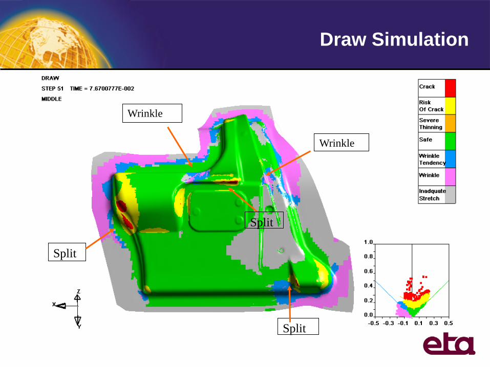
Wrinkle
Wrinkle
Split
Split
Split
Draw Simulation

Draw Simulation

Class A Surface
Major Strain
Minor Strain

Evaluation of the Trimline Layout
Cam trim area
Cam trim area

Addendum shape adjusted area
Addendum Shape Adjustment

Cad Data Received
Draw station
Flange station

Simulation Setup
Draw station
Flange station
Trim station

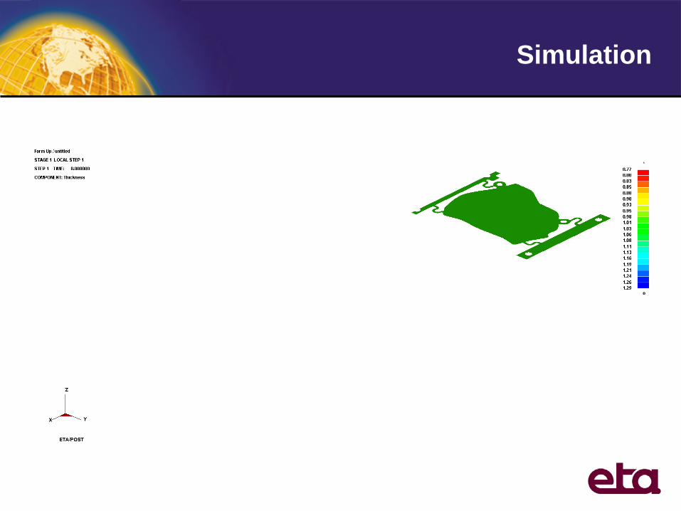
Overview (FLD)

Overview (Thickness Contour)
Alternate view


Data Received
Draw Station
Pre-form Station
Re-Draw Station

FLD Plot

Simulation

Blank Thickness After Re-draw
Areas of Thinning
Areas of Thinning
Areas of Thickening
Areas of Thickening
Simulation

Springback Prediction
Red – beforeGreen- after

Springback Prediction
Red – beforeGreen- after
Original tool - grey

Compensation: Tool Shape Morph
Reverse the Tool shape based on Springback results

Before
Results Before & After Compensation
After 1 Re-cut
Courtesy of Continental Tool and Die

Contour Before and After Compensation
Courtesy of Continental Tool and Die
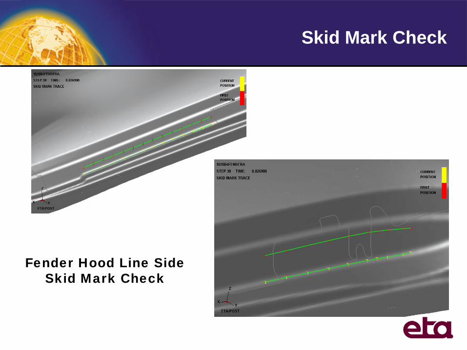
Skid Mark Check
Fender Hood Line Side Skid Mark Check

Result of Initial Blank Outline Result of Developed Blank Outline
Initial OutlineDeveloped Outline
Blank Development: Corner Cut Off

Trimline Development
Iteration 1
Iteration 2
Iteration 3

Local regions on the trim line
Local Trim Line Development
OP10: Forming OP20: Trimming OP30: Forming
The segment 2 on the target
The segment 1 on the target

Commonly Asked Questions
• Can simulation help me determine how many toolset do I need to make this part?
• What is the dynamic affect?
• What about the rate effects?
• How accurate is the simulation results?

www.formingsimulation.com 44
Execution Time
• Execution time primarily depends on:– material properties– mesh size– number of elements– contacts– speed of computer
• CPU estimation– Time step ∆t = minimum ∆x/c– number of cycles = termination time / ∆t – CPU time = (# cycles)(# elements)(time per zone cycle)– correction is needed for time step reduction– correction is needed for number and size of contacts

Dynamic effects
• Mass induced : inertia forces, usually have a small influence for slow processes but can be artificially increased due to the use of certain numerical techniques
• Material induced : viscosity or so-called strain rate effects, can be important depending upon the material, may need specific numerical treatment if the process is too slow to be simulated ‘real time’

The issue of spurious inertia
• CPU time is proportional to the number of timesteps
• In order to reduce cpu time we need to either reduce the termination time ( = increase tool speed ) or increase the timestep :
tTcpu∆
≈
↑=↑⇒∆
↑↓⇒
↓⇒ El
Elt
vT
cpu cc ρ
ρ
= Cycles

Critical (or minimum) time step size:
where C is the sound wave propagation speed in 3D-continuum:
Ct minmin
l=∆
( )( )( )ρυυ
υ211
1
−+−
=E
C
Time Step

The methods
• Consider the kinetic energy in the deformable structure ( = blank ) :
• Suppose we want to reduce the cpu time by a factor a>1 :
• Reducing the cpu by a factor a will increase the kinetic energy by a-squared !
2
2mvke =
→⇒→⇒→⇒∆→∆
→⇒→⇒→⇒→
22
222
22
22
22
2
mvamvmamatat
mvamvavvaTT
acpucpu
ρρ

Consequence for the application
• For a quasistatic and /or slow dynamic process ( such as stamping) we need to make sure that the ‘numerical’ ke des not influence the solution
• Need to get the same answer for 2 different ( low enough) speeds
• This is illustrated in : LS-Dyna Mat 36 Regularization Investigation: AL 6060Update ( Anthony Smith, Honda R&D, LS-DYNA conference Detroit 2014 )

Mat 24 – ELFORM 16
50
10 m/s, SP 10 m/s, DP
2 m/s, SP 2 m/s, DP

Mat 24 – ELFORM 16
51
1 m/s, SP 1 m/s, DP
0.5 m/s, SP
0.5 m/s, DP
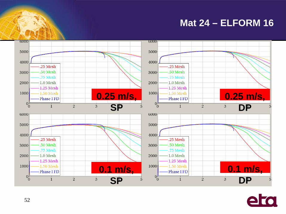
Mat 24 – ELFORM 16
52
0.25 m/s, SP
0.25 m/s, DP
0.1 m/s, SP
0.1 m/s, DP

Mat 24 , ELFORM 16
53
Nominal Velocity: Exact Velocity:
Strain Rate: # Cycles SP
Region?QS
Region?m/s m/s s-1
10 10.664 426.56 25512 YES NO
2 2.1328 85.312 127563 YES NO
1 1.0664 42.656 255125 NO NO
0.5 0.5332 21.328 510263 NO YES
0.25 0.2666 10.664 1020513 NO YES
0.1 0.10664 4.2656 2551394 NO YES

Rate effects
• What if viscosity influences the material response for strain rates < 1/s ?
• Use of ‘SCALE’ in MAT_260A and MAT_260B in LS-DYNA :
• This is the way to assess rate dependency for low rate values while performing a simulation at higher velocity then physical
• Very reliable for displacement driven problems

Example from LS-DYNA manual

Conclusion
• Simulation has strength and limitations
• Effectiveness of the simulation relay on the understanding of the technology properly

Future
• Highly interactive preprocessor will allow user design tooling surface virtually
• Obtain simulation result instantly
• Optimized process and design will be possible through large database system
Recommended