Introduction to Data ScienceGIRI NARASIMHAN, SCIS, FIU

Giri Narasimhan
Clustering
6/26/18
!2

Giri Narasimhan
Clustering dogs using height & weight
6/26/18
!3

Giri Narasimhan
Clustering dogs using height & weight
6/26/18
!4
Giri Narasimhan
Clustering
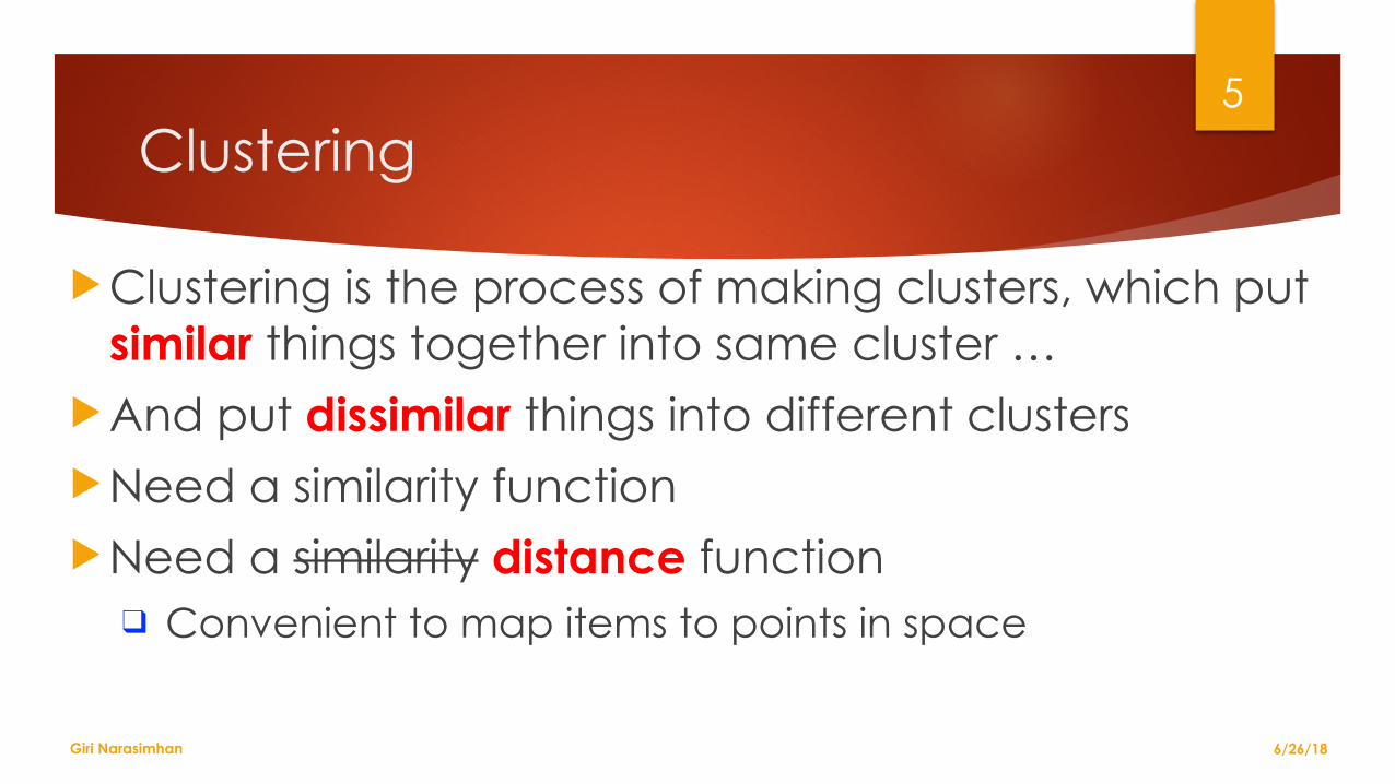
!Clustering is the process of making clusters, which put similar things together into same cluster …
!And put dissimilar things into different clusters !Need a similarity function !Need a similarity distance function
❑ Convenient to map items to points in space
6/26/18
!5

Giri Narasimhan
Distance Functions
! Jaccard Distance ! Hamming Distance ! Euclidean Distance ! Cosine Distance ! Edit Distance ! …
! What is a distance function ❑ D(x,y) >= 0 ❑ D(x,y) = D(y,x) ❑ D(x,y) <= D(x,z) + D(z,y)
6/26/18
!6

Giri Narasimhan
Clustering Strategies
! Hierarchical or Agglomerative ❑ Bottom-up
! Partitioning methods ❑ Top-down
! Density-based ! Cluster-based ! Iterative methods
6/26/18
!7
Giri Narasimhan
Curse of Dimensionality
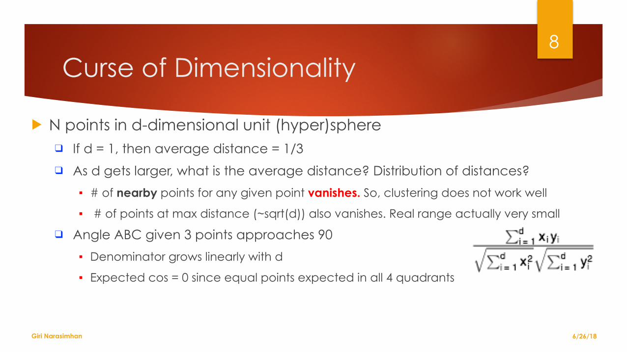
! N points in d-dimensional unit (hyper)sphere ❑ If d = 1, then average distance = 1/3 ❑ As d gets larger, what is the average distance? Distribution of distances?
▪ # of nearby points for any given point vanishes. So, clustering does not work well ▪ # of points at max distance (~sqrt(d)) also vanishes. Real range actually very small
❑ Angle ABC given 3 points approaches 90 ▪ Denominator grows linearly with d ▪ Expected cos = 0 since equal points expected in all 4 quadrants
6/26/18
!8

Giri Narasimhan
Hierarchical Clustering
6/26/18
!9

Giri Narasimhan
Hierarchical Clustering
! Starts with each item in different clusters ! Bottom up ! In each iteration
❑ Two clusters are identified and merged into one ! Items are combined as the algorithm progresses ! Questions:
❑ How are clusters represented ❑ How to decide which ones to merge ❑ What is the sopping condition
! Typical algorithm: find smallest distance between nodes of different clusters
6/26/18
!10

Giri Narasimhan
Hierarchical Clustering248 CHAPTER 7. CLUSTERING
(7,10)
(9,3)
(11,4)
(12,6)
(5,2)(2,2)
(3,4)
(12,3)
(4,8)
(4,10)
(4,9)
(10,5)
(2.5, 3)
(6,8)
(4.7, 8.7)
(10.5, 3.8)
Figure 7.5: Three more steps of the hierarchical clustering
1. Takethedistancebetween two clusters to be theminimum of thedistancesbetween any two points, one chosen from each cluster. For example, inFig. 7.3 wewould next chose to cluster the point (10,5) with the cluster oftwo points, since (10,5) has distance
√2, and no other pair of unclustered
points is that close. Note that in Example 7.2, we did make this combi-nat ion eventually, but not unt il we had combined another pair of points.In general, it is possible that this rule will result in an ent i rely differentclustering from that obtained using the distance-of-centroids rule.
2. Take the distance between two clusters to be the average distance of allpairs of points, one from each cluster.
(2,2) (3,4) (5,2) (4,8) (4,10) (6,8) (7,10) (11,4) (12,3) (10,5) (9,3) (12,6)
Figure 7.6: Tree showing the complete grouping of the points of Fig. 7.2
6/26/18
!11

Giri Narasimhan
Output of Clustering: Dendrogram
248 CHAPTER 7. CLUSTERING
(7,10)
(9,3)
(11,4)
(12,6)
(5,2)(2,2)
(3,4)
(12,3)
(4,8)
(4,10)
(4,9)
(10,5)
(2.5, 3)
(6,8)
(4.7, 8.7)
(10.5, 3.8)
Figure 7.5: Three more steps of the hierarchical clustering
1. Takethedistancebetween two clusters to be theminimum of thedistancesbetween any two points, one chosen from each cluster. For example, inFig. 7.3 wewould next chose to cluster the point (10,5) with the cluster oftwo points, since (10,5) has distance
√2, and no other pair of unclustered
points is that close. Note that in Example 7.2, we did make this combi-nat ion eventually, but not unt il we had combined another pair of points.In general, it is possible that this rule will result in an ent i rely differentclustering from that obtained using the distance-of-cent roids rule.
2. Take the distance between two clusters to be the average distance of allpairs of points, one from each cluster.
(2,2) (3,4) (5,2) (4,8) (4,10) (6,8) (7,10) (11,4) (12,3) (10,5) (9,3) (12,6)
Figure 7.6: Tree showing the complete grouping of the points of Fig. 7.26/26/18
!12
248 CHAPTER 7. CLUSTERING
(7,10)
(9,3)
(11,4)
(12,6)
(5,2)(2,2)
(3,4)
(12,3)
(4,8)
(4,10)
(4,9)
(10,5)
(2.5, 3)
(6,8)
(4.7, 8.7)
(10.5, 3.8)
Figure 7.5: Three more steps of the hierarchical clustering
1. Takethedistancebetween two clusters to be theminimum of thedistancesbetween any two points, one chosen from each cluster. For example, inFig. 7.3 wewould next chose to cluster the point (10,5) with the cluster oftwo points, since (10,5) has distance
√2, and no other pair of unclustered
points is that close. Note that in Example 7.2, we did make this combi-nat ion eventually, but not unt il we had combined another pair of points.In general, it is possible that this rule will result in an ent i rely differentclustering from that obtained using the distance-of-centroids rule.
2. Take the distance between two clusters to be the average distance of allpairs of points, one from each cluster.
(2,2) (3,4) (5,2) (4,8) (4,10) (6,8) (7,10) (11,4) (12,3) (10,5) (9,3) (12,6)
Figure 7.6: Tree showing the complete grouping of the points of Fig. 7.2

Giri Narasimhan
Measures for a cluster
! Radius: largest distance from a centroid ! Diameter: largest distance between some pair of points in cluster ! Density: # of points per unit volume ! Volume: some power of radius or diameter ! Tightness, separation, … ! Good cluster: when diameter of each cluster is much larger than its
nearest cluster or nearest point outside cluster
6/26/18
!13
Giri Narasimhan
Stopping condition for clustering
! Cluster radius or diameter crosses a threshold ! Cluster density drops below a certain threshold ! Ratio of diameter to distance to nearest cluster drops below a certain
threshold
6/26/18
!14

Giri Narasimhan
K-Means Clustering
6/26/18
!15

CAP5510 / CGS 5166 2/11/13
!16
Start
Example from Andrew Moore’s tutorial on Clustering.

CAP5510 / CGS 5166 2/11/13
!17
Example from Andrew Moore’s tutorial on Clustering.

CAP5510 / CGS 5166 2/11/13
!18
Example from Andrew Moore’s tutorial on Clustering.

CAP5510 / CGS 5166 2/11/13
!19
Start
End
Example from Andrew Moore’s tutorial on Clustering.

CAP5510 / CGS 5166 2/11/13
!20K-Means Clustering [McQueen ’67]
Repeat ❑ Start with randomly chosen cluster centers
❑ Assign points to give greatest increase in score
❑ Recompute cluster centers
❑ Reassign points
until (no changes) Try the applet at: http://home.dei.polimi.it/matteucc/Clustering/tutorial_html/AppletH.html

Giri Narasimhan
How to find K for K-means?
6/26/18
!21
CAP5510 / CGS 5166 2/11/13
!22Comparisons
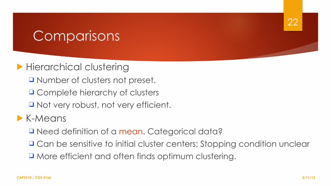
! Hierarchical clustering ❑ Number of clusters not preset. ❑ Complete hierarchy of clusters ❑ Not very robust, not very efficient.
! K-Means ❑ Need definition of a mean. Categorical data? ❑ Can be sensitive to initial cluster centers; Stopping condition unclear ❑ More efficient and often finds optimum clustering.

Giri Narasimhan
Implementing Clustering
6/26/18
!23

Giri Narasimhan
Example High-Dim Application: SkyCat
!A catalog of 2 billion “sky objects” represents objects by their radiation in 7 dimensions (frequency bands).
!Problem: cluster into similar objects, e.g., galaxies, nearby stars, quasars, etc.
!Sloan Sky Survey is a newer, better version.
6/26/18
!24

Giri Narasimhan
Curse of Dimensionality
!Assume random points within a bounding box, e.g., values between 0 and 1 in each dimension.
! In 2 dimensions: a variety of distances between 0 and 1.41.
! In 10,000 dimensions, the difference in any one dimension is distributed as a triangle.
6/26/18
!25

Giri Narasimhan
How to find K for K-means?
6/26/18
!26

Giri Narasimhan
BFR Algorithm
!BFR (Bradley-Fayyad-Reina) – variant of K -means for very large (disk-resident) data sets.
!Assumes that clusters are normally distributed around a centroid in Euclidean space. ❑ SDs in different dimensions may vary
6/26/18
!27

Giri Narasimhan
BFR … 2
! Points read “chunk” at a time. ! Most points from previous chunks summarized by simple
statistics. ! First load handled by some sensible approach:
1. Take small random sample and cluster optimally. 2. Take sample; pick random point, & k – 1 more points
incrementally, each as far from previously points as possible.
6/26/18
!28

Giri Narasimhan
BFR … 3
1. Discard set : points close enough to a centroid to be summarized.
2. Compression set : groups of points that are close together but not close to any centroid. They are summarized, but not assigned to a cluster.
3. Retained set : isolated points.
6/26/18
!29

Giri Narasimhan
BFR … 4
6/26/18
!30

Giri Narasimhan
BFR: How to summarize?
! Discard Set & Compression Set: N, SUM, SUMSQ ! 2d + 1 values ! Average easy to compute
❑ SUM/N
! SD not too hard to compute ❑ VARIANCE = (SUMSQ/N) – (SUM/N)2
6/26/18
!31

Giri Narasimhan
BFR: Processing
! Maintain N, SUM, SUMSQ for clusters ! Policies for merging compressed sets needed and for merging a point in
a cluster ! Last chunk handled differently
❑ Merge all compressed sets ❑ Merge all retained sets into nearest clusters
! BFR suggests Mahalanobis Distance
6/26/18
!32

Giri Narasimhan
Mahalanobis Distance
! Normalized Euclidean distance from centroid. ! For point (x1,…,xk) and centroid (c1,…,ck):
1. Normalize in each dimension: yi = (xi -ci)/σi
2. Take sum of the squares of the yi ’s.
3. Take the square root. ! For Gaussian clusters, ~65% of points within SD dist
6/26/18
!33

Giri Narasimhan
GRPGF Algorithm
6/26/18
!34

Giri Narasimhan
GRPGF Algorithm
! Works for non-Euclidean distances ! Efficient, but approximate ! Works well for high dimensional data
❑ Exploits orthogonality property for high dim data
! Rules for splitting and merging clusters
6/26/18
!35

Giri Narasimhan
Clustering for Streams
! BDMO (authors, B. Babcock, M. Datar, R. Motwani, & L. O’Callaghan) ! Points of stream partitioned into, and summarized by, buckets with sizes
equal to powers of two. Size of bucket is number of points it represents. ! Sizes of buckets obey restriction that <= two of each size. Sizes are
required to form a sequence -- each size twice previous size, e.g., 3,6,12,24,... .
! Bucket sizes restrained to be nondecreasing as we go back in time. As in Section 4.6, we can conclude that there will be O(log N) buckets.
! Rules for initializing, merging and splitting buckets
6/26/18
!36
Recommended