Interference effects of choice on confidence: Quantumcharacteristics of evidence accumulationPeter D. Kvama,b,1, Timothy J. Pleskacb,1, Shuli Yua, and Jerome R. Busemeyerc
aDepartment of Psychology, Michigan State University, East Lansing, MI 48824; bCenter for Adaptive Rationality, Max Planck Institute for HumanDevelopment, 14195 Berlin, Germany; and cDepartment of Psychological and Brain Sciences, Indiana University, Bloomington, IN 47405
Edited by James L. McClelland, Stanford University, Stanford, CA, and approved July 10, 2015 (received for review January 13, 2015)
Decision-making relies on a process of evidence accumulation whichgenerates support for possible hypotheses. Models of this processderived from classical stochastic theories assume that informationaccumulates by moving across definite levels of evidence, carving outa single trajectory across these levels over time. In contrast, quantumdecision models assume that evidence develops over time in asuperposition state analogous to a wavelike pattern and that judg-ments and decisions are constructed by a measurement process bywhich a definite state of evidence is created from this indefinitestate. This constructive process implies that interference effectsshould arise when multiple responses (measurements) are elicitedover time. We report such an interference effect during a motiondirection discrimination task. Decisions during the task interferedwith subsequent confidence judgments, resulting in less extremeand more accurate judgments than when no decision was elicited.These results provide qualitative and quantitative support for aquantum random walk model of evidence accumulation over thepopular Markov random walk model. We discuss the cognitive andneural implications of modeling evidence accumulation as a quantumdynamic system.
confidence | Markov | decision-making | cognitive model | random walk
Decisions in a wide range of tasks (e.g., inferring the presenceor absence of a disease, the guilt or innocence of a suspect,
and the left or right direction of enemy movement) require evidenceto be accumulated in support of different hypotheses. Arguably, themost successful theory of evidence accumulation in humans andother animals is Markov random walk (MRW) theory (and diffu-sion models, their continuous space extensions) (1, 2). MRWs canbe viewed as psychological implementations of a first-order Bayes-ian inference process that assigns a posterior probability to eachhypothesis (3). MRWs can account for choices, response times, andconfidence for a variety of different decision types (2, 4). Moreover,these models of the accumulation process have been connected toneural activity during decision-making (5, 6).According to MRW models, when deciding between two hy-
potheses, the cumulative evidence for or against each hypothesisrealizes different levels at different times to generate a single par-ticle-like trajectory of evidence levels across time (Fig. 1). At anypoint in time, the decision-maker has a definite level of evidence,and choices are made by comparing the existing level of evidenceagainst a criterion. Evidence above the criterion favors one option,and evidence below it favors the alternative. Other responses aremodeled in a similar manner; for example, confidence ratings aremodeled by mapping evidence states onto one or more ratings (4).However, this idea that judgments and decisions are simply read outfrom the existing level of evidence—henceforth referred to as the“read-out” assumption—is inconsistent with the well-establishedidea that preferences and beliefs are constructed rather thanrevealed by judgments and decisions (7).We present an alternative model of choice and judgment based
on quantum random walk (QRW) theory (8–11), which posits thatpreferences and beliefs are constructed when a judgment or de-cision is made. Note that this work does not make the assumptionthat the brain is a quantum computer; instead, we simply use themathematics of quantum theory to explain and predict human
behavior. According to QRW theory, at any point in time before adecision, the decision-maker is in a superposition state that is notlocated at a single level of evidence. Instead, each level of evidencehas a potential to be expressed, formalized as a probability ampli-tude (Fig. 1). New information changes the amplitudes, producing awavelike process that moves the amplitude distribution across time.In some ways the QRW is like a second-order Bayesian model
(12). According to the latter, the decision-maker assigns a proba-bility (rather than an amplitude) to each level of evidence for eachhypothesis. However, like the MRW model, second-order Bayesianmodels are perfectly compatible with the read-out assumption, andas an optimal model, this would suggest that a decision should notchange the probability assigned to each evidence level. In contrast, aQRW, like all quantum models of cognition (13), treats a judgmentor decision as a measurement process that constructs a definite statefrom an indefinite (superposition) state. When a decision is made,the indefinite state collapses onto a set of evidence levels that cor-respond to the observed choice, producing a definite choice state.Confidence ratings work similarly, with the indefinite state collapsingonto a more specific set of levels corresponding to the observed rating.These different theories of choice and judgment have strong
implications for sequences of responses. Consider the situationwhen decision-makers have to make a choice (e.g., decide thathypothesis A or B is true) and later rate their confidence that agiven (usually the chosen) hypothesis is true. According to theread-out assumption, a choice is reported on the basis of existingevidence that does not change the internal state of evidence itself.This applies to the MRW, a second-order Bayesian model, andmany other accumulation models as well. Thus, after poolingacross a person’s choices, the distribution of confidence ratingsshould be identical to conditions in which the person makesno choice at all. By contrast, the state of the system in a QRW
Significance
Most cognitive and neural decision-making models—owing totheir roots in classical probability theory—assume that decisionsare read out of a definite state of accumulated evidence. Thisassumption contradicts the view held by many behavioral scien-tists that decisions construct rather than reveal beliefs and pref-erences. We present a quantum random walk model of decision-making that treats judgments and decisions as a constructivemeasurement process, and we report the results of an experimentshowing that making a decision changes subsequent distributionsof confidence relative to when no decision is made. This findingprovides strong empirical support for a parameter-free predictionof the quantum model.
Author contributions: P.D.K., T.J.P., and J.R.B. conceived of the study; P.D.K., T.J.P., .S.Y.,and J.R.B. designed the research; P.D.K. ran the study; P.D.K. and T.J.P. analyzed data; P.D.K.,T.J.P., S.Y., and J.R.B. wrote the paper; and T.J.P. supervised all aspects of the work.
The authors declare no conflict of interest.
This article is a PNAS Direct Submission.
Freely available online through the PNAS open access option.1To whom correspondence may be addressed. Email: [email protected] or [email protected].
This article contains supporting information online at www.pnas.org/lookup/suppl/doi:10.1073/pnas.1500688112/-/DCSupplemental.
www.pnas.org/cgi/doi/10.1073/pnas.1500688112 PNAS | August 25, 2015 | vol. 112 | no. 34 | 10645–10650
PSYC
HOLO
GICALAND
COGNITIVESC
IENCE
SAPP
LIED
MATH
EMATICS

is changed when a choice creates a definite state. Subsequentprocessing starts from the definite state, and the amplitudesspread out again. Thus, if information processing continues afterthe initial stage, the QRW predicts an interference effect wherethe marginal distribution of confidence judgments following achoice will differ from a condition in which no choice is made.A proof of the predicted interference effect for QRWs is in SI
Appendix. The proof shows that the interference effect of choice onconfidence is the result of the interaction between the creation of adefinite state and subsequent evidence accumulation after making achoice. Subsequent or second-stage processing is a necessary con-dition for the effect. Critically, second-stage processing occurs whenpeople are asked to report a confidence rating following a choice,giving rise to response reversals (14) and other properties (15). Wealso provide a proof that MRWs predict no difference between themarginal distributions of confidence ratings (i.e., no interference)regardless of the presence of second-stage processing. This proofholds for a large range of MRWs, including ones with decay (16),leakage of evidence (17), and trial-by-trial variability in the decisionprocess (18).
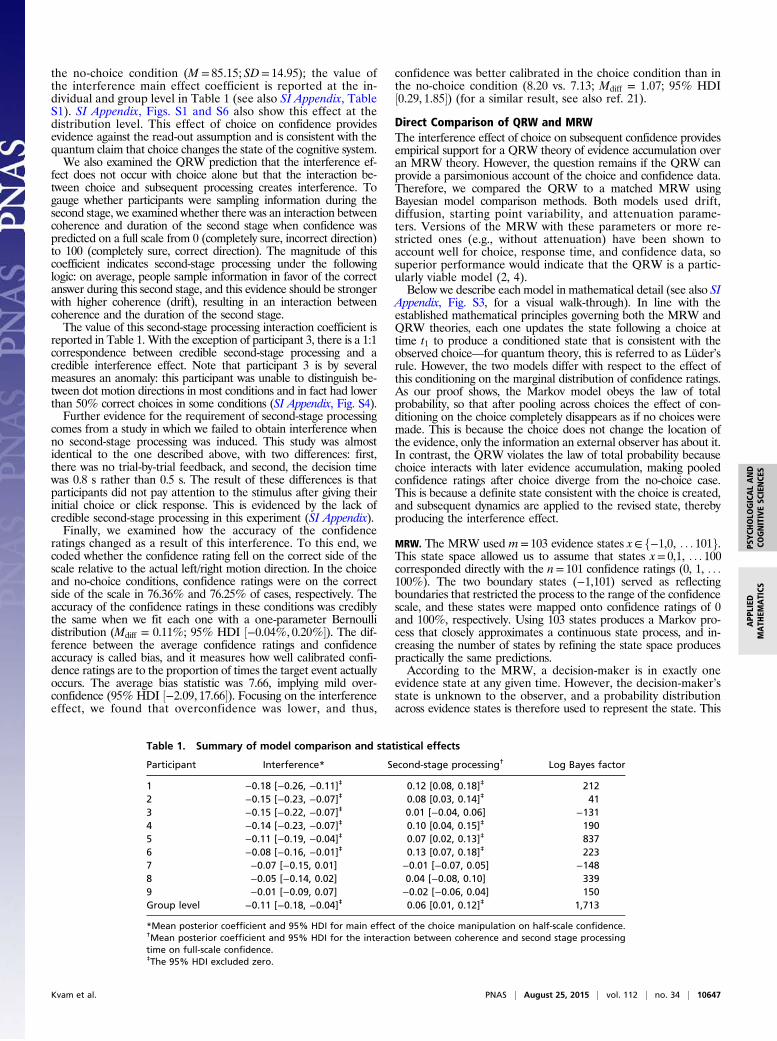
Empirical Test of Predicted Interference EffectWe tested these opposing predictions concerning interferenceeffects using a perceptual task that requires participants to judgethe direction of motion in a dynamic dot display (Fig. 2). Spe-cifically, nine participants completed 112 blocks of 24 trials eachover five 1-h experimental sessions, a total of 2,688 trials perperson (SI Appendix). During each trial, participants viewed arandom dot motion stimulus that consisted of moving white dotsin a circular aperture on a black background (19). A percentageof the dots moved coherently in one direction (left or right), and therest moved randomly. Difficulty was manipulated between trials bychanging the percentage of coherently moving dots (2%, 4%, 8%,
or 16%). In the choice condition—half of the randomly orderedblocks—participants were prompted 0.5 s from stimulus onset via alow-frequency beep (400 Hz) to decide whether the coherentlymoving dots were moving left or right and entered their choiceby clicking the corresponding mouse button. In the no-choicecondition—the other half of the blocks—participants wereprompted 0.5 s from stimulus onset via a high-frequency beep(800 Hz) to make a motor response (click the left or right mousebutton as instructed). In all trials, the stimulus remained onscreen for a second stage of processing after the choice or click.After an additional 0.05, 0.75, or 1.5 s following the first re-sponse, participants were prompted via a second beep (400 Hz)to rate their confidence that the coherently moving dots weremoving right on a semicircular scale that appeared at the time ofthe prompt, ranging from 0 (certain left) to 100% (certain right)in unit steps. Note that to match the overall processing time ofthe stimulus across conditions, the confidence prompt was time-locked to the initial choice or click entry.For the behavioral analyses, we collapsed confidence responses
across the dot motion direction, recoding confidence onto a half scale(50% guess to 100% certain). All behavioral analyses were conductedusing hierarchical Bayesian general linear models (20). The co-efficient b is the linear effect of a predictor on the criterion. We alsoreport the highest density interval (HDI) for all estimates, whichspecifies the range covering the 95% most credible values of theposterior estimates. A normal link was used for confidence judgmentsafter transforming them to log odds, and a logistic link was used forchoices.On average, confidence increased with motion coherence
(b= 0.66; 95% HDI = ½0.31, 1.02�). In the choice condition, theproportion of correct choices increased with coherence(b= 0.50; 95% HDI = ½0.04, 1.16�). Confidence judgments were,on average, lower in the choice (M = 83.96; SD= 15.56) than in
40 50 60 70 800% 10 20 30 90 100%‘Certain
Left’‘CertainRight’
40 50 60 70 800% 10 20 30 90 100%‘Certain
Left’‘CertainRight’
Markov Random Walk Quantum Random Walk
Fig. 1. Diagram of a state representation of a Markov and a quantum random walk model. In the Markov model, evidence (shaded state) evolves over timeby moving from state to state, occupying one definite evidence level at any given time. In the quantum model the decision-maker is in an indefinite evidencestate, with each evidence level having a probability amplitude (shadings) at each point in time.
ChoiceCondition
No ChoiceCondition
Choose
Click
t1 t2
You earned 75 points.
Your choice was correct.
Your click was correct.
You earned 75 points.
0 100
50
1020
30 40 60 708090
t0
0 100
50
1020
30 40 60 708090
Fig. 2. Diagram of the task. A fixation point indicated the choice/no-choice condition, then the stimulus was shown for 0.5 s. A prompt (t1) then asked for adecision on the direction of the dot motion (choice condition) or a motor response (no-choice condition). The stimulus remained on the screen. A secondprompt (t2) then asked for a confidence rating on the direction of the dot motion. Finally, feedback was given on the accuracy of their responses.
10646 | www.pnas.org/cgi/doi/10.1073/pnas.1500688112 Kvam et al.
the no-choice condition (M = 85.15; SD= 14.95); the value ofthe interference main effect coefficient is reported at the in-dividual and group level in Table 1 (see also SI Appendix, TableS1). SI Appendix, Figs. S1 and S6 also show this effect at thedistribution level. This effect of choice on confidence providesevidence against the read-out assumption and is consistent with thequantum claim that choice changes the state of the cognitive system.We also examined the QRW prediction that the interference ef-
fect does not occur with choice alone but that the interaction be-tween choice and subsequent processing creates interference. Togauge whether participants were sampling information during thesecond stage, we examined whether there was an interaction betweencoherence and duration of the second stage when confidence waspredicted on a full scale from 0 (completely sure, incorrect direction)to 100 (completely sure, correct direction). The magnitude of thiscoefficient indicates second-stage processing under the followinglogic: on average, people sample information in favor of the correctanswer during this second stage, and this evidence should be strongerwith higher coherence (drift), resulting in an interaction betweencoherence and the duration of the second stage.The value of this second-stage processing interaction coefficient is
reported in Table 1. With the exception of participant 3, there is a 1:1correspondence between credible second-stage processing and acredible interference effect. Note that participant 3 is by severalmeasures an anomaly: this participant was unable to distinguish be-tween dot motion directions in most conditions and in fact had lowerthan 50% correct choices in some conditions (SI Appendix, Fig. S4).Further evidence for the requirement of second-stage processing
comes from a study in which we failed to obtain interference whenno second-stage processing was induced. This study was almostidentical to the one described above, with two differences: first,there was no trial-by-trial feedback, and second, the decision timewas 0.8 s rather than 0.5 s. The result of these differences is thatparticipants did not pay attention to the stimulus after giving theirinitial choice or click response. This is evidenced by the lack ofcredible second-stage processing in this experiment (SI Appendix).Finally, we examined how the accuracy of the confidence
ratings changed as a result of this interference. To this end, wecoded whether the confidence rating fell on the correct side of thescale relative to the actual left/right motion direction. In the choiceand no-choice conditions, confidence ratings were on the correctside of the scale in 76.36% and 76.25% of cases, respectively. Theaccuracy of the confidence ratings in these conditions was crediblythe same when we fit each one with a one-parameter Bernoullidistribution (Mdiff = 0.11%; 95% HDI ½−0.04%, 0.20%�). The dif-ference between the average confidence ratings and confidenceaccuracy is called bias, and it measures how well calibrated confi-dence ratings are to the proportion of times the target event actuallyoccurs. The average bias statistic was 7.66, implying mild over-confidence (95% HDI ½−2.09, 17.66�). Focusing on the interferenceeffect, we found that overconfidence was lower, and thus,
confidence was better calibrated in the choice condition than inthe no-choice condition (8.20 vs. 7.13; Mdiff = 1.07; 95% HDI½0.29, 1.85�) (for a similar result, see also ref. 21).
Direct Comparison of QRW and MRWThe interference effect of choice on subsequent confidence providesempirical support for a QRW theory of evidence accumulation overan MRW theory. However, the question remains if the QRW canprovide a parsimonious account of the choice and confidence data.Therefore, we compared the QRW to a matched MRW usingBayesian model comparison methods. Both models used drift,diffusion, starting point variability, and attenuation parame-ters. Versions of the MRW with these parameters or more re-stricted ones (e.g., without attenuation) have been shown toaccount well for choice, response time, and confidence data, sosuperior performance would indicate that the QRW is a partic-ularly viable model (2, 4).Below we describe each model in mathematical detail (see also SI
Appendix, Fig. S3, for a visual walk-through). In line with theestablished mathematical principles governing both the MRW andQRW theories, each one updates the state following a choice attime t1 to produce a conditioned state that is consistent with theobserved choice—for quantum theory, this is referred to as Lüder’srule. However, the two models differ with respect to the effect ofthis conditioning on the marginal distribution of confidence ratings.As our proof shows, the Markov model obeys the law of totalprobability, so that after pooling across choices the effect of con-ditioning on the choice completely disappears as if no choices weremade. This is because the choice does not change the location ofthe evidence, only the information an external observer has about it.In contrast, the QRW violates the law of total probability becausechoice interacts with later evidence accumulation, making pooledconfidence ratings after choice diverge from the no-choice case.This is because a definite state consistent with the choice is created,and subsequent dynamics are applied to the revised state, therebyproducing the interference effect.
MRW. The MRW used m= 103 evidence states x∈ f−1,0, . . . 101g.This state space allowed us to assume that states x= 0,1, . . . 100corresponded directly with the n= 101 confidence ratings (0, 1, . . .100%). The two boundary states (−1,101) served as reflectingboundaries that restricted the process to the range of the confidencescale, and these states were mapped onto confidence ratings of 0and 100%, respectively. Using 103 states produces a Markov pro-cess that closely approximates a continuous state process, and in-creasing the number of states by refining the state space producespractically the same predictions.According to the MRW, a decision-maker is in exactly one
evidence state at any given time. However, the decision-maker’sstate is unknown to the observer, and a probability distributionacross evidence states is therefore used to represent the state. This
Table 1. Summary of model comparison and statistical effects
Participant Interference* Second-stage processing† Log Bayes factor
1 −0.18 [−0.26, −0.11]‡ 0.12 [0.08, 0.18]‡ 2122 −0.15 [−0.23, −0.07]‡ 0.08 [0.03, 0.14]‡ 413 −0.15 [−0.22, −0.07]‡ 0.01 [−0.04, 0.06] −1314 −0.14 [−0.23, −0.07]‡ 0.10 [0.04, 0.15]‡ 1905 −0.11 [−0.19, −0.04]‡ 0.07 [0.02, 0.13]‡ 8376 −0.08 [−0.16, −0.01]‡ 0.13 [0.07, 0.18]‡ 2237 −0.07 [−0.15, 0.01] −0.01 [−0.07, 0.05] −1488 −0.05 [−0.14, 0.02] 0.04 [−0.08, 0.10] 3399 −0.01 [−0.09, 0.07] −0.02 [−0.06, 0.04] 150Group level −0.11 [−0.18, −0.04]‡ 0.06 [0.01, 0.12]‡ 1,713
*Mean posterior coefficient and 95% HDI for main effect of the choice manipulation on half-scale confidence.†Mean posterior coefficient and 95% HDI for the interaction between coherence and second stage processingtime on full-scale confidence.‡The 95% HDI excluded zero.
Kvam et al. PNAS | August 25, 2015 | vol. 112 | no. 34 | 10647
PSYC
HOLO
GICALAND
COGNITIVESC
IENCE
SAPP
LIED
MATH
EMATICS

distribution is defined by a mixed state vector ϕðtÞ of dimensionm× 1, which gives the probability of being in state x at time t,
PrðxjtÞ=ϕxðtÞ. [1]
The probability distribution ϕð0Þ specifies the decision-mak-er’s initial state, which is set as a uniform distribution centeredon x= 50. The width w is a free parameter indexing trial-by-trialvariability in the initial state.As the decision-maker considers information, the process
moves from state to state. An m×m transition matrix P specifiesthe probability that the process moves from one state to anotherafter some period, so that the probability distribution over evi-dence states after time t is
ϕðtÞ=PðtÞ ·ϕð0Þ. [2]
Choice probability and confidence are determined as follows.Define a response operator MR, which is a diagonal matrix with0.5 located in the row for confidence level 50, ones located inrows for confidence levels 51 through 101, and zeros otherwise.The probability of choosing right at time t1, denoted pðRjt1Þ,equals the sum of the projection MR ·ϕðt1Þ. The probability ofchoosing left at time t1 is 1− pðRjt1Þ. If right motion is chosen,then this provides information on the location of the evidence(e.g., evidence is at or above state 50), and the probability dis-tribution over the states is updated to ϕðt1jRÞ=MR ·ϕðt1Þ
pðRjt1Þ . Note thatif a person were to choose left motion, the response operator MRwould be replaced by ML; the two are identical except that the1 and 0 entries along the main diagonal are flipped.For confidence ratings, define My as a diagonal matrix with 1
located in the row(s) corresponding to confidence y and zerosotherwise. In the choice condition, the probability of choosingconfidence level y at time t2 following a right motion choice thenequals the sum of the projection My ·Pðt2Þ ·ϕðt1jRÞ. In the no-choice condition, the probability of choosing confidence level yat time t2 equals the sum of the projection My ·ϕðt2Þ.The transition matrix is constructed from an m×m intensity
matrix Q using the Kolmogorov forward equation so that
PðtÞ= expðQtγÞ, [3]
where exp is the matrix exponential function and γ is a parameterdescribing the proportion of time spent processing information up totime t. Consistent with recent work in modeling postdecisional pro-cessing (15), this was set to γ = 1 during the first stage of processing(t0 to t1) but was free to vary during the second stage to account forattenuation in incoming information following the first response.The entries qj,k of the intensity matrix are
qj,j =−σ2, [4a]
qj−1,j =12�σ2 − δ
�, [4b]
qj+1,j =12�σ2 + δ
�. [4c]
This definition of the intensity matrix was chosen so that thediscrete state Markov process closely approximates a continuousstate Wiener diffusion process (8). The drift rate δ determinesthe probability that the process steps toward the true dot motiondirection. We scaled the drift rate directly from the percentageof coherently c moving dots so that
δ= μ · c. [5]
If the dots are moving left, c is negative. The parameter μ is afree parameter indexing sensitivity to the coherence. The
parameter σ2 is a diffusion rate controlling the dispersion ofthe process. This MRW operates on a finite state space, so weset the states x=−1 and x= 101 as reflecting boundaries to allowthe process to continue its evolution after it reaches the finitelimits, −q1,1 = q1,2 = σ2 and q102,103 =−q103,103 = σ2.
QRW. The QRW also usedm= 103 evidence states as in the MRW,similarly assuming that states x= 0,1, . . . 100 corresponded directlywith the 101 confidence ratings and that states x=−1 and x= 101were reflecting boundaries which mapped onto confidence ratingsof 0 and 100%.According to the QRW, a decision-maker is not necessarily in any
one evidence state at any given time. This uncertainty on the part ofthe decision-maker is modeled with a superposition state vector ψðtÞof size m× 1, which gives the probability amplitude at the xth evi-dence level at time t. The probability of observing state x at time t isthe squared length of the amplitude in the corresponding row:
PrðxjtÞ= jψ xðtÞj2. [6]
The state vector ψð0Þ specifies the initial superposed evidencestate. We set the probability amplitudes across these states tobe uniformly and symmetrically distributed around x= 50. Thewidth w of this distribution is a free parameter representinginitial uncertainty.As information is processed, the superposition state drifts over
time until a response is elicited. The m×m unitary matrix op-erator U evolves the amplitudes over time, so that
ψðtÞ=UðtÞ ·ψð0Þ. [7]
Choice probability and confidence are determined as follows.We define MR in a similar manner as in the MRW. It is a di-agonal matrix with 1ffiffi
2p in the row for confidence level 50, ones
located in rows for confidence levels 51 through 101, and zerosotherwise. The probability of choosing right at time t1, denotedPrðRjt1Þ, equals the squared length of the projection MR ·ψðt1Þ.The probability of choosing left is 1−PrðRjt1Þ. If right motion ischosen, the superposition state is projected onto the corre-sponding evidence levels, and the probability amplitude isupdated to ψðt1jRÞ= MR ·ψðt1Þffiffiffiffiffiffiffiffiffiffiffiffi
PrðRjt1Þp . If left motion is chosen, MR is
replaced by ML; the two are identical except that the 1 and0 entries along the main diagonal are flipped.Subsequent processing starts from this new state so that in the
choice condition the probability of choosing confidence level y attime t2 after choosing right then equals the squared length of theprojection My ·Uðt2Þ ·ψðt1jRÞ. In the no-choice condition, no pro-jection is done at t1, and the probability of choosing confidence levely at time t2 equals the squared length of the projection My ·ψðt2Þ.The unitary matrix is constructed from a Hamiltonian matrix
H using the Schrödinger equation so that
UðtÞ= expð−itHγÞ. [8]
The attenuation parameter γ operates in the same way as in theMRW. The entries hj,k of the Hamiltonian matrix are
hj,j = δ · j=m, [9a]
hj−1,j = hj+1,j = σ2. [9b]
This definition of the Hamiltonian matrix was chosen so thatthe discrete state quantum process closely approximates thecontinuous state Schrödinger process (9). The δ and σ2 parametersof the QRW have a similar effect as their counterparts in the MRWbut function differently. The diffusion coefficient σ2 controls therate at which amplitude flows out of the states. The drift rate δdetermines the rate at which probability amplitude flows in. Thedrift rate δ was set to be a multiplicative function of coherence
10648 | www.pnas.org/cgi/doi/10.1073/pnas.1500688112 Kvam et al.

(Eq. 5). [Eq. 9 is a linear potential function in the diagonal of theHamiltonian (multiplying drift by the state index) so there is aconstant positive force pushing evidence toward the correct di-rection. However, other potential functions (e.g., quadratic) shouldbe investigated in the future.]The interference effect arises because the amplitudes in states
0–50 interact with those in 50–100 in the no-choice condition,pushing each other outward toward more extreme evidence states.This pressure is not present in the choice condition, leading to lessextreme evidence and hence confidence ratings. One consequenceof these less extreme confidence ratings is less overconfidence in thechoice condition.
Model Comparison. Each model has four free parameters: a pa-rameter that sets the drift as a scalar function of motion directioncoherence (μ), a diffusion parameter (σ2), a second-stage attenua-tion parameter that dampens of the rate of incoming informationafter making a choice (γ), and a parameter that determines thewidth of the initial state distribution (starting point variability) (w)(SI Appendix, Table S3). Non-decision time parameters, accountingfor components of the response time exogenous to the evidenceaccumulation process, had limited influence on model fits andwere dropped in order to facilitate model estimation.The models were compared at the individual level: for each
participant and each model, four parameters were used to accountfor 2,688 trials across 24 experimental conditions. Despite havingthe same number of parameters, the QRW may be functionallymore complex, allowing it to produce good fits to the data withoutnecessarily bearing any relationship to the underlying process. Toaccount for this, we compared the Bayes factor between the twomodels for each participant (22).The Bayes factor was calculated using a fine-grid approxima-
tion across all possible combinations of the four parameters tocompute the likelihood function and uniform priors over theirvalues. The results are summarized in Table 1; the log Bayesfactor indicates the log odds of the QRW model over the MRWgiven the data (see SI Appendix, Tables S4 and S5, for themaximum likelihoods and parameter estimates).The Bayes factor for seven out of nine participants and the group
level factor decisively favored the QRW (maximum likelihoodsyield the same conclusion). Participant 7 did not show second-stageprocessing or an interference effect, so the MRWmay well describethe behavior of this participant. Participant 3 was unable to distin-guish between dot motion directions in many conditions, which
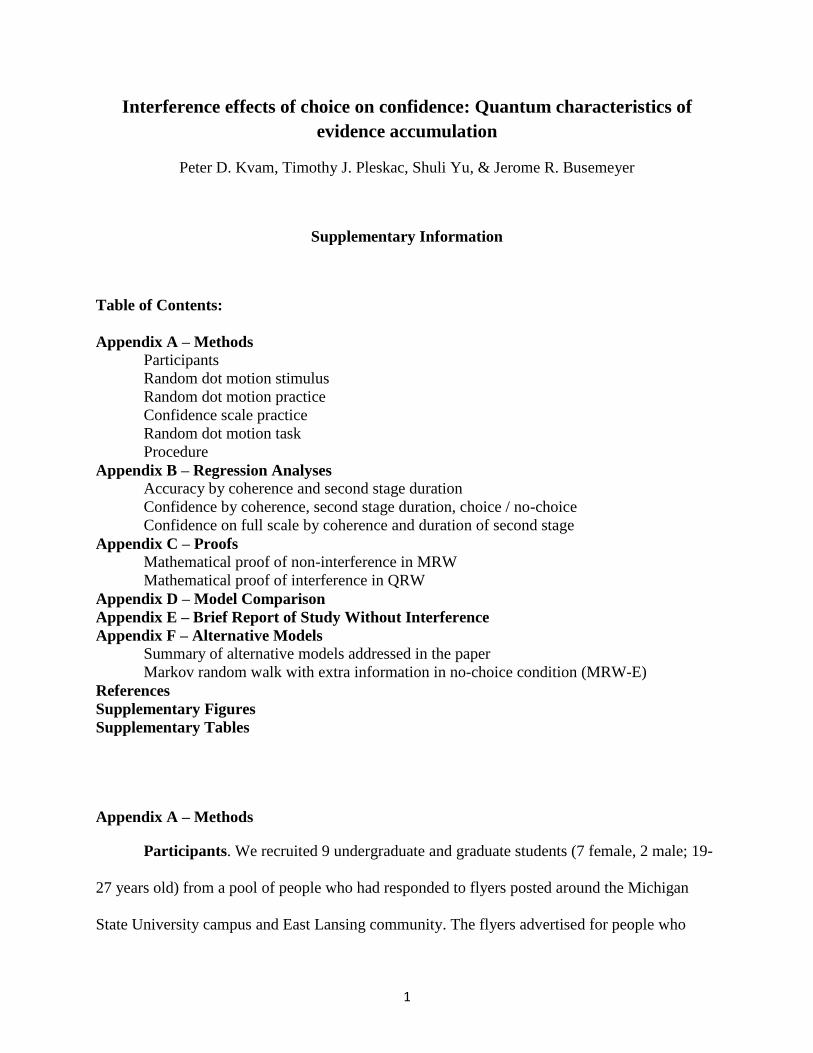
caused difficulty in fitting both models (SI Appendix, Fig. S4). Fu-ture model development incorporating methods for mapping evi-dence to confidence (e.g., using only 0/10/20% or 0/50/100%ratings) could potentially improve fits, but this does not affect in-terference so we favor simpler, more parsimonious models here.Fig. 3 illustrates the fit of each model to the choice proportions for
each coherence condition and the distribution of confidence in thechoice and no-choice conditions for one participant and coherencelevel [all participants across conditions are given in SI Appendix, Fig.S4 (see also SI Appendix, Figs. S5 and S6)]. There are several reasonsthat the QRW gives a better account of the data than the MRW.First, the MRW predicts identical marginal distributions of confi-dence ratings between choice and no-choice conditions, whereas thequantum model picks up the slight rightward shift of these ratings inthe no-choice condition; this phenomenon is the interference effectwe described (see SI Appendix, Fig. S6; the QRW posterior pre-dictions yield a group mean shift in confidence of +0.66%, comparedto +1.19% in the data). Second, the QRW was often better able tosimultaneously capture choices along with confidence ratings acrossthe various conditions, whereas the MRW often had to sacrifice orcompromise between the two. Notably, the MRW underestimatedchoice proportions because higher diffusion more accurately cap-tured confidence distributions but at the cost of predicting lowerchoice accuracy. Finally, the observed confidence distributions arefrequently multimodal and discontinuous. The MRW again does notaccount for these properties. By contrast, the QRW accounts for allof these characteristics in a parsimonious way, operating only on itsfirst principles to earn a superior Bayes factor.Although this MRW and similar versions have been used to
model a wide range of choice and judgment data, it may struggleto account for this data simply because it cannot account for theinterference effect. To examine this possibility, we tested a sec-ond model—the MRW-E—which assumes that additional evi-dence may have been accumulated in the no-choice condition,producing more extreme confidence ratings and thus an in-terference effect. Despite the added ability to produce in-terference, the QRW still outperformed the MRW-E. The Bayesfactor for seven out of nine participants and the group level factoragain decisively favored the QRW over the MRW-E. In comparisonwith the MRW, the MRW-E provides a largely equivalent or oftenpoorer fit in terms of Bayes factors (SI Appendix, Table S6 and Fig.S7). Part of the reason the MRW-E does poorly, in addition to thecharacteristics it inherits from the MRW, is that it assumes moreevidence is accumulated in the no-choice condition producing a
Fig. 3. Data and model fits for participant 4 with coherence level 8%.
Kvam et al. PNAS | August 25, 2015 | vol. 112 | no. 34 | 10649
PSYC
HOLO
GICALAND
COGNITIVESC
IENCE
SAPP
LIED
MATH
EMATICS

change in the accuracy of the confidence ratings as well as the meanshift in confidence. Recall, however, that there is no credible changein the accuracy of the confidence ratings in the data.
DiscussionIn this paper, we have developed a model of evidence accumulationduring judgment and decision-making based on quantum randomwalk theory. The QRW represents a point of departure in modelingevidence accumulation from the more typical classical probabilityapproach. In the classical case, evidence evolves over time, butjudgments and decisions are simply read out from an existing statewithout changing the internal state of evidence. In the quantumcase, evidence also evolves over time, but judgments and decisionsare measurements that create a new definite state from an in-definite (superposition) state. This quantum perspective recon-ceptualizes how we model uncertainty and formalizes a long-heldhypothesis that judgments and decisions create rather than revealpreferences and beliefs. The different approaches make competinga priori predictions for the effect of sequences of responses, andwe have shown strong empirical support for the quantum predic-tion that choices interfere with subsequent confidence judgments.Moreover, we have shown for the first time to our knowledge thatthe QRW is a viable competitor to the MRW in quantitativelyfitting choice and confidence distributions. Note that the QRW canalso account for response time distributions (8) and can out-perform Markov models in this area as well (10).A pertinent question is whether the MRW can be adapted to
account for the phenomena we observed. This is certainly possiblebut may prove difficult: as we have shown, our results provideseveral constraints on potential adaptations. The interference effectitself is a strong constraint: many versions of the MRW that com-monly give good accounts of choice and confidence data do notpredict any interference.A second constraint is how the interference effect occurred. In
particular, confidence was less extreme following a choice. This posesa problem for explanations like the confirmation bias, where peoplefocus on evidence that justifies their decision after making a choice,meaning they should be more confident in the choice condition(23, 24). Moreover, confidence accuracy also did not change. Thisposes a problem for models like the MRW-E that assume differentamounts of processing between the choice and no-choice conditions.A third constraint is that the interference effect only occurred
when there was second-stage processing. This result poses problemsfor explanations based on differences in the mapping of evidenceonto confidence (25) and explanations assuming that the act ofmaking a choice introduces error into the cognitive system. Both
explanations would fail to explain why choice alone (withoutsecond-stage processing) does not interfere with confidence.Alternatively, on some trials during the choice condition, par-ticipants reversed their initial choice (14) and could havereported unexpectedly low confidence on these trials, producingthe interference effect. However, reversals during the choicecondition happened infrequently (6.1%), and confidence onreversal trials was only slightly lower than on consistent trials.We discuss this and other alternative models in more detail inSI Appendix, section F.Although an alternative MRW may be found to account for our
results, this does not diminish the QRW’s significance in high-lighting and challenging important assumptions regarding thejudgment and decision-making process. In this paper, we haveshown that a common assumption of cognitive and neural theoriesof decision-making—the read-out assumption—is violated even in asimple perceptual task. An interference effect occurred when par-ticipants were asked to make a decision about the leftward orrightward motion of a stimulus. Specifically, their subsequent con-fidence estimates were more conservative than when no earlierdecision was made, and they were consequently less overconfident.This result, along with quantitatively superior model fits, lendsstrong support to the modeling of choice and confidence as aquantum random walk process, a model which describes decision-making as a constructive process wherein a definite state is createdfrom an indefinite superposition. In addition to the cognitive im-plications, a QRW model of evidence accumulation potentiallysidesteps the problem of how a group of neurons can produceobserved behavior that is consistent with a single evidence accu-mulation trajectory (26). The QRW suggests that the mismatchmight lie in the cognitive representation of evidence accumulation:instead of treating evidence accumulation as a single trajectory, itmay be more accurate to conceptualize it as a wavelike superposi-tion state. In fact, populations of interacting neurons processingevidence in parallel can give rise to a quantum random walk like theone presented here (10), and similar population coding modelswould certainly be capable of carrying out the necessary operations(27). Hence, quantum random walk theory provides a previouslyunexamined perspective on the nature of the evidence accumula-tion process that underlies both cognitive and neural theoriesof decision-making.
ACKNOWLEDGMENTS. This work was supported by grants from the NationalScience Foundation (NSF) (0955140) (to T.J.P.) and Air Force Office ofScientific Research (FA9550-12-1-0397) (to J.R.B.). P.D.K. was supported bya graduate fellowship from the NSF (1424871).
1. Gold JI, Shadlen MN (2007) The neural basis of decision making. Annu Rev Neurosci30:535–574.
2. Ratcliff R, Smith PL (2004) A comparison of sequential sampling models for two-choicereaction time. Psychol Rev 111(2):333–367.
3. Bogacz R, Brown E, Moehlis J, Holmes P, Cohen JD (2006) The physics of optimaldecision making: A formal analysis of models of performance in two-alternativeforced-choice tasks. Psychol Rev 113(4):700–765.
4. Pleskac TJ, Busemeyer JR (2010) Two-stage dynamic signal detection: A theory ofchoice, decision time, and confidence. Psychol Rev 117(3):864–901.
5. Hanes DP, Schall JD (1996) Neural control of voluntary movement initiation. Science274(5286):427–430.
6. Shadlen MN, NewsomeWT (2001) Neural basis of a perceptual decision in the parietalcortex (area LIP) of the rhesus monkey. J Neurophysiol 86(4):1916–1936.
7. Lichtenstein S, Slovic P, eds (2006) The Construction of Preference (Cambridge UnivPress, Cambridge, UK).
8. Busemeyer JR, Wang Z, Townsend JT (2006) Quantum dynamics of human decision-making. J Math Psychol 50(3):220–241.
9. Feynman RP, Leighton RB, Sands M (2013) The Feynman Lectures on Physics, DesktopEdition (Basic Books, New York), Vol I.
10. Fuss IG, Navarro DJ (2013) Open parallel cooperative and competitive decision pro-cesses: A potential provenance for quantum probability decision models. Top CognSci 5(4):818–843.
11. Kempe J (2003) Quantum random walks: An introductory overview. Contemp Phys44(4):307–327.
12. Ma WJ, Beck JM, Latham PE, Pouget A (2006) Bayesian inference with probabilisticpopulation codes. Nat Neurosci 9(11):1432–1438.
13. Busemeyer JR, Bruza P (2012)QuantumModels of Cognition and Decision (CambridgeUniv Press, Cambridge, UK).
14. Resulaj A, Kiani R, Wolpert DM, Shadlen MN (2009) Changes of mind in decision-
making. Nature 461(7261):263–266.15. Yu S, Pleskac TJ, Zeigenfuse MD (2015) Dynamics of postdecisional processing of
confidence. J Exp Psychol Gen 144(2):489–510.16. Busemeyer JR, Townsend JT (1993) Decision field theory: A dynamic-cognitive ap-
proach to decision making in an uncertain environment. Psychol Rev 100(3):432–459.17. Usher M, McClelland JL (2001) The time course of perceptual choice: The leaky,
competing accumulator model. Psychol Rev 108(3):550–592.18. Ratcliff R, Rouder JN (1998) Modeling response times for two-choice decisions. Psychol
Sci 9(5):347–356.19. Ball K, Sekuler R (1987) Direction-specific improvement in motion discrimination.
Vision Res 27(6):953–965.20. Kruschke J (2010) Doing Bayesian Data Analysis: A Tutorial Introduction with R (Ac-
ademic, Waltham, MA).21. Sniezek JA, Paese PW, Switzer FS, III (1990) The effect of choosing on confidence in
choice. Organ Behav Hum Decis Process 46(2):264–282.22. Kass RE, Raftery AE (1995) Bayes factors. J Am Stat Assoc 90(430):773–795.23. Koriat A, Lichtenstein S, Fischhoff B (1980) Reasons for confidence. J Exp Psychol Learn
Mem Cogn 6(2):107–118.24. Zylberberg A, Barttfeld P, Sigman M (2012) The construction of confidence in a
perceptual decision. Front Integr Neurosci 6:79.25. Green DM, Swets JA (1966) Signal Detection Theory and Psychophysics (Wiley, New
York), Vol 1.26. Zandbelt B, Purcell BA, Palmeri TJ, Logan GD, Schall JD (2014) Response times from
ensembles of accumulators. Proc Natl Acad Sci USA 111(7):2848–2853.27. Pouget A, Dayan P, Zemel R (2000) Information processing with population codes. Nat
Rev Neurosci 1(2):125–132.
10650 | www.pnas.org/cgi/doi/10.1073/pnas.1500688112 Kvam et al.
1
Interference effects of choice on confidence: Quantum characteristics of
evidence accumulation
Peter D. Kvam, Timothy J. Pleskac, Shuli Yu, & Jerome R. Busemeyer
Supplementary Information
Table of Contents:
Appendix A – Methods
Participants
Random dot motion stimulus
Random dot motion practice
Confidence scale practice
Random dot motion task
Procedure
Appendix B – Regression Analyses
Accuracy by coherence and second stage duration
Confidence by coherence, second stage duration, choice / no-choice
Confidence on full scale by coherence and duration of second stage
Appendix C – Proofs
Mathematical proof of non-interference in MRW
Mathematical proof of interference in QRW
Appendix D – Model Comparison
Appendix E – Brief Report of Study Without Interference
Appendix F – Alternative Models
Summary of alternative models addressed in the paper
Markov random walk with extra information in no-choice condition (MRW-E)
References
Supplementary Figures
Supplementary Tables
Appendix A – Methods
Participants. We recruited 9 undergraduate and graduate students (7 female, 2 male; 19-
27 years old) from a pool of people who had responded to flyers posted around the Michigan
State University campus and East Lansing community. The flyers advertised for people who

2
wanted to participate in paid studies on judgment and decision making. An additional 2
participants did not return after the first session, so they were excluded from further analyses.
Participants were paid $8 per hour and could receive up to $5 more based on how many points
they earned divided by the number of points it was possible to earn.
Random dot motion (RDM) stimulus. The motion display was similar to that used in
previous neuropsychological studies [1,2,3]. The RDM stimulus consisted of a field of white
moving dots on a black background, presented on a circular aperture of 10° diameter. There were
three interleaved sets of dots such that each set was re-plotted three video frames later, On each
iteration of the same set, some percentage of the dots were displaced by .25° to produce apparent
motion at 5°/s velocity, while the remaining dots were plotted at random locations. The
probability that a specific dot was displayed in motion is termed motion coherence. We used four
levels of motion coherence: 2%, 4%, 8%, and 16%. The task was programmed using the
Psychtoolbox extensions [4,5].
RDM practice (Session 1). The purpose of this task was to train participants to make
timely responses immediately after hearing an auditory cue. During a given trial, a RDM
stimulus appeared on screen and participants pressed either the left mouse button () or the right
button () to indicate which direction they believed a majority of the dots were moving. First,
they did 5 trials where they could make their decision response at any time. They also did 10
trials of prompted decision training, in which they were instructed to enter their decision
immediately after a 400 Hz beep that took place at either 0.5 or 1.0 s after stimulus onset. After
each trial, participants were given feedback about their decision accuracy and timing (responses
more than 500ms after the beep were met with a prompt to try to respond faster).
Confidence scale practice (Session 1). Participants completed a series of trials to

3
become familiar with entering a confidence rating with the mouse. During a given trial a fixation
display was shown for 500ms, then a percentage value (e.g., 9%) appeared just below the center
of the screen. The semicircular confidence rating scale (see Fig. 2), used to control for the
distance traveled to select a confidence rating with the mouse, also appeared onscreen above the
percentage value. Participants moved the cursor with the mouse from the center of the screen to
the appropriate point on the scale to match the value as quickly and accurately as possible. The
value of the confidence rating was randomized and participants continued until they achieved at
least 10 answers that were within 2 percentage points of the correct number.
In addition, participants saw 15 trials of the random dot motion task with no mouse click
element included – 5 trials in which they could simply enter a confidence rating when they saw
fit, and 10 trials in which they were prompted with a beep to make a confidence response. This
400 Hz beep occurred at 1.0 or 2.0 s following stimulus onset.
RDM direction discrimination task. The time course of a trial for the choice and no-
choice conditions is shown at the top and bottom (respectively) of Figure 2. Participants would
start each trial of the task by clicking on a small fixation shape, which was either a circle (during
choice trials) or a square (during no-choice trials). Once clicked (centering the mouse cursor), it
would persist for 0.3 s before the RDM stimulus came on-screen and the mouse cursor was
removed from the screen. In the choice condition, participants were cued via a low frequency
beep (400 Hz) at 0.5 s from stimulus onset to choose which direction the majority of the dots
were moving, left or right. Participants recorded their choice by pressing either the left or right
mouse button. In the no-choice condition, participants were cued via a high frequency beep (800
Hz) at 0.5 s from stimulus onset to click either the left or right mouse button. The mouse button
was specified at the beginning of that block of trials (the left or right mouse button specification
4
alternated between blocks). A different frequency beep was used to minimize any confusion
participants experienced between the two conditions.
After participants made their choice or clicked the button, a semi-circular confidence scale
(from 0 to 100%, with major demarcations at 10 point intervals and minor demarcations at every
1; see main text, Fig. 2) appeared over the upper half of the field of dots. The confidence scale
was in terms of the confidence the dots were moving right, i.e., confidence of 0% indicated
participants were certain the dots were moving left and a confidence of 100% indicated
participants were certain the dots were moving right. Confidence judgments were cued at 0.05,
0.75, or 1.5 s after the initial choice or click response was entered.
Procedure. During the first session, participants first received a presentation describing
the task that they were about to do. This included a description of all conditions and response
modes. These directions were repeated on-screen during the training described above, which
enabled them to practice making decisions and using the confidence scale. In addition, at the end
of their first session, they saw a plot comparing dot coherence against their choice accuracy
along with a Weibull fit line. We explained this plot to participants, noting that it should be an
increasing function (it was for all participants in this experiment).
At the beginning of each session, in addition to the training trials described in the sections
above, participants would do 10 trials each of the choice and no-choice conditions. These were
organized into 4 blocks (2 choice, 2 no-choice) so participants could get accustomed to the task
once again before we collected new data.
The different conditions were organized into blocks of trials such that each block
contained 2 iterations of each of the 4 levels of dot coherence (2 / 4 / 8 / 16%) crossed with each
of the 3 levels of the duration of the second stage of processing (0.05 / 0.75 / 1.5 s) for a total of

5
24 trials / block. Half of these blocks were choice blocks, where the pre-trial fixation was a red
circle (see main text Fig. 2) with a 400 Hz beep to prompt a choice response after 500ms of
stimulus presentation. The other half were no-choice blocks, where the pre-trial fixation was a
red square and a 800Hz beep prompted them to click the right button on half of the no-choice
blocks and the left button on the other half of the no-choice blocks (i.e. 2/4 blocks were choice,
1/4 were click-right, 1/4 were click-left). They were informed prior to the start of each block as
to which type it would be. Mean response times after t1 for the choice condition were 0.548
(Median = 0.370, SD = 0.625) s for the choice condition and 0.383 (Median = 0.298, SD =
0.333) s for the no-choice condition. After t2, confidence response times were 0.767 (Median =
0. 863, SD = 0.392) s for the choice condition and 0.767 (Median = 0.871, SD = 0.391) s for the
no-choice condition.
After each trial, participants received feedback about whether their click was correct
(whether their choice was correct on choice trials, or whether they clicked in the requested
direction on the no-choice trials) as well as how many points they received for their confidence
response. The amount of points participants received from their confidence rating was
determined using a linear transformation of the Brier scoring rule [6]:
Score = 100 * [c – (conf / 100)]2.
The variable c indicates the correct answer (0 for left, 1 for right) and conf indicates their
response on the absolute scale (0 for certain left, 100 for certain right). The Brier scoring rule is
a strictly proper scoring rule, meaning that the optimal strategy on the part of the participant is to
provide a probability estimate that matches one’s true subjective probabilities.
Appendix B – Regression Analyses

6
All regression analyses used hierarchical Bayesian linear models that included all
possible interactions between predictors ([7], chapter 14). Vague priors were used for each
parameter so as to let the data have maximal influence on the posterior estimates. We report the
mean estimate of the slope parameter corresponding to a predictor (b) as well as the interval that
contains the 95% most credible values for this parameter (Highest Density Interval / HDI). In
practice, these highest density intervals tended to be fairly similar to the estimates one would
obtain for a 95% confidence interval, but were slightly stricter (were closer to 0 than a
corresponding classical confidence interval).
Linear regression analyses all used MATLAB, JAGS, and matjags to fit the model. Each
analysis was estimated using 8 parallel chains. Each chain was comprised of 1000 burn-in steps
(unrecorded samples to allow the chain to reach the reasonable parameter space) and 10,000
samples. Preliminary analyses confirmed that all chains converged. Each of the analyses reported
in the paper are described individually below:
Accuracy by coherence and second stage duration. Choice accuracy in the choice
condition was predicted by coherence level, the duration of the second stage, and their
interaction. A logit link function was used for this analysis.
Confidence by coherence, second stage duration, choice/no-choice. In order to gauge
how confidence changed over the different conditions, we transformed confidence responses so
that they reflected how sure a participant was of the direction of dot motion, i.e. collapsed across
directions in which they could respond. This resulted in confidence responses (y) ranging from
50% (unsure of motion direction) to 100% (certain of motion direction) based on raw responses

7
(r) from the 0 (certain left) to 100 (certain right) scale. The cumulative distributions of
confidence for each individual on this scale is shown in Figure S1.
100 , 50
, 50
r ry
r r
Coherence, duration of second stage, and the choice / no-choice manipulation were used
as predictors. Fig. S2 below plots how mean confidence changes over each of these
manipulations. Table S1 lists the mean group level coefficients and their HDI’s for each of the
experimental factors: IJT duration, degree of motion coherence, and the choice/no choice
manipulation.
Confidence on full scale by coherence and duration of second stage. The interference
effect relies on second stage processing in order to appear – there should be some change in
confidence over time after t1 and the magnitude of this change should depend on the coherence
of the stimuli, which implies an interaction between the duration of the second stage and dot
motion coherence. During this second stage, we assume information about the state of the
stimulus continues to be sampled and accumulated [8]. This suggests that additional information
should lead to higher levels of confidence when accumulated evidence already favors the correct
answer at t1. However, when accumulated evidence reflects the incorrect answer at t1, new
information should conflict with the existing information, on average decreasing a person’s
confidence [8,9]. These conflicting forces reduce the effect of second stage processing time on
confidence when it is coded on a half-scale, resulting in a null effect of second stage processing
time x coherence as reported in Table S1. However, the effect of second stage processing can be
much better seen if confidence ratings discriminate between correct and incorrect responses. To
8
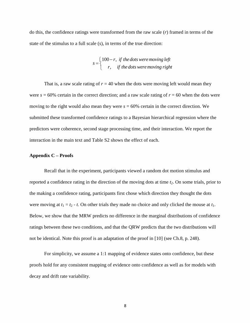
do this, the confidence ratings were transformed from the raw scale (r) framed in terms of the
state of the stimulus to a full scale (s), in terms of the true direction:
That is, a raw scale rating of r = 40 when the dots were moving left would mean they
were s = 60% certain in the correct direction; and a raw scale rating of r = 60 when the dots were
moving to the right would also mean they were s = 60% certain in the correct direction. We
submitted these transformed confidence ratings to a Bayesian hierarchical regression where the
predictors were coherence, second stage processing time, and their interaction. We report the
interaction in the main text and Table S2 shows the effect of each.
Appendix C – Proofs
Recall that in the experiment, participants viewed a random dot motion stimulus and
reported a confidence rating in the direction of the moving dots at time t2. On some trials, prior to
the making a confidence rating, participants first chose which direction they thought the dots
were moving at t1 = t2 - t. On other trials they made no choice and only clicked the mouse at t1.
Below, we show that the MRW predicts no difference in the marginal distributions of confidence
ratings between these two conditions, and that the QRW predicts that the two distributions will
not be identical. Note this proof is an adaptation of the proof in [10] (see Ch.8, p. 248).
For simplicity, we assume a 1:1 mapping of evidence states onto confidence, but these
proofs hold for any consistent mapping of evidence onto confidence as well as for models with
decay and drift rate variability.
100 ,
,
r if thedots weremoving lefts
r if thedots weremoving right
9
Mathematical proof of non-interference in MRW. The MRW predicts that the
marginal distribution of confidence ratings in the two conditions (choice and no choice) should
be equal, Pr(conf = y|t2, choice) = Pr(conf = y|t2, no-choice). To see this, we define three m × m
state to response probability transition matrices. The first, Mcorrect, is for choosing correctly and
is filled with zeroes everywhere except for a series of ones along the main diagonal in rows
corresponding to confidence levels 51-100 and a ½ at the row corresponding to confidence level
50. The second, Mincorrect, is for choosing incorrectly. It is filled with zeroes everywhere except
for ones along the main diagonal in rows representing levels 0-49 and a ½ at the row
corresponding to confidence level 50. The third, My, is used to give the probability of a
confidence rating y and is entirely zeroes except for a one in cell corresponding to confidence
rating y. It is important to note, however, that the proof shown below does not depend on these
specifications for Mcorrect and Mincorrect. The proof is valid for any Mcorrect and Mincorrect that have
positive entries and satisfy the following completeness requirement Mcorrect + Mincorrect = I , where
I is the identity matrix. Thus the proof holds for a much more general class of measurements at
choice than the specific model that we fit to the data. Finally, let L be a 1 × m matrix filled with
ones, which we use to sum the values across states.
In the choice condition, the probability of giving a particular confidence rating y at time t2
after a choice (at t1) is simply the marginal sum across correct and incorrect answers, which we
can show is equivalent to the probability of giving confidence rating y at t2 in the no-choice
condition:

10
2
1 2 1 2
1 1
1 1
Pr( | , )
Pr( at at ) Pr( at at )
[ ( ) ( ) (0) ( ) ( ) (0)]
( ) [ ( ) (0) ( ) (0)]
y correct y incorrect
y correct incorrect
conf y t choice
correct t conf y t incorrect t conf y t
t t t t
t t t
L M P M P M P M P
L M P M P M P
1
1
2
( ) ( ) (0)
( ) (0)
Pr( | , )
y
y
t t
t t
conf y t no choice
L M P I P
L M P
As we can see, the MRW must obey the law of total probability (in this context, this is
called the Chapman – Kolmogorov equation) for every confidence level y, and therefore it
predicts that the marginal distribution of confidence ratings between the choice and no-choice
conditions should be identical. The same prediction holds when the transition matrix is non-
stationary, as can be seen by replacing P(t) with P(ti, tj). Note the prediction does assume the
initial state (0) is the same for both conditions. It also assumes that the transition matrices do
not change across conditions; however, the transition matrices could change across time and the
same conclusion would follow.
Mathematical proof of interference in QRW. To see the predicted violation of the law
of total probability (i.e., the interference effect), we define three state-response amplitude
transition matrices: Mcorrect, Mincorrect, and My. These matrices are equivalent everywhere to the
corresponding state probability transition matrices for the MRW described earlier, with the
exception that there is a 1
2 placed in the row corresponding to confidence level 50 for Mcorrect
and Mincorrect. In the QRW, each of these matrices is a projection operator that collapses a vector
onto the subspace spanned by the corresponding basis states. This means that when we take the
11
squared magnitude of each entry (element-wise), Mcorrect + Mincorrect = I (the combined correct
and incorrect projection operators include all possible responses).
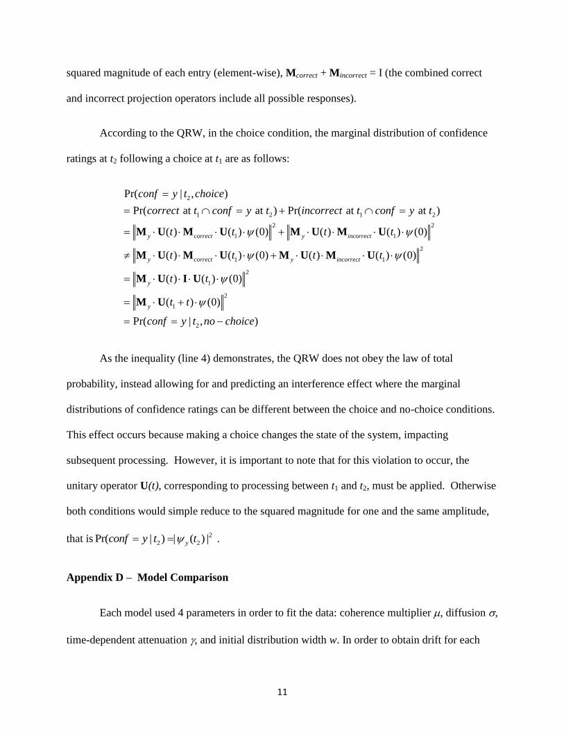
According to the QRW, in the choice condition, the marginal distribution of confidence
ratings at t2 following a choice at t1 are as follows:
2
1 2 1 2
2 2
1 1
1 1
Pr( | , )
Pr( at at ) Pr( at at )
( ) ( ) (0) ( ) ( ) (0)
( ) ( ) (0) ( ) ( ) (
y correct y incorrect
y correct y incorrect
conf y t choice
correct t conf y t incorrect t conf y t
t t t t
t t t t
M U M U M U M U
M U M U M U M U2
2
1
2
1
2
0)
( ) ( ) (0)
( ) (0)
Pr( | , )
y
y
t t
t t
conf y t no choice
M U I U
M U
As the inequality (line 4) demonstrates, the QRW does not obey the law of total
probability, instead allowing for and predicting an interference effect where the marginal
distributions of confidence ratings can be different between the choice and no-choice conditions.
This effect occurs because making a choice changes the state of the system, impacting
subsequent processing. However, it is important to note that for this violation to occur, the
unitary operator U(t), corresponding to processing between t1 and t2, must be applied. Otherwise
both conditions would simple reduce to the squared magnitude for one and the same amplitude,
that is2
2 2Pr( | ) | ( ) |yconf y t t .
Appendix D – Model Comparison
Each model used 4 parameters in order to fit the data: coherence multiplier , diffusion ,
time-dependent attenuation , and initial distribution width w. In order to obtain drift for each

12
coherence level, we multiply the drift coefficient by each coherence 2, 4, 8, 16%), giving 4 levels
of drift for each drift parameter. Initially, we included parameters corresponding to non-decision
and non-judgment time, but these were dropped because they drastically increased the
computational demands of model fitting without substantially contributing to model
performance.
Note that in the Markov model we present in the paper, we set the decision bounds to -1
and 101 and the step size Δ to 1, resulting in equations 4a-c and 5. However, to draw it closer to
the typical Markov approximation of a Wiener diffusion model, which uses bounds of -1 and 1,
one could set Δ = 1/51 and begin the process at state 0. For each time they occur in the model
description, we would then set σ = σ·Δ (σ2 = σ
2·Δ
2) and µ = µ·Δ (δ = µ·c·Δ) (see [11]).
In order to fit the models and compute a Bayes factor between them, we took a grid of 21
drift, diffusion, and attenuation parameters and 51 initial distribution parameters and calculated
the log of the multinomial function at each point in order to form a 21 x 21 x 21 x 51 grid
approximation of the likelihood function:

13
ln[𝑃𝑟(𝐷 | 𝑀𝑜𝑑𝑒𝑙)]
= ∑ ∑ (𝑛𝑐𝑜𝑟𝑟,𝑐,𝑖 ∙ ln[Pr(𝑐𝑜𝑟𝑟|𝑀𝑜𝑑𝑒𝑙, 𝑡1, 𝑐, 𝑖)] + 𝑛𝑖𝑛𝑐𝑜𝑟𝑟,𝑐,𝑖
3
𝑖=1
4
𝑐=1
∙ ln[Pr(𝑖𝑛𝑐𝑜𝑟𝑟|𝑀𝑜𝑑𝑒𝑙, 𝑡1, 𝑐, 𝑖)]
+ [∑ 𝑟𝑐ℎ𝑜𝑖𝑐𝑒,𝑐𝑜𝑟𝑟,𝑐,𝑖,𝑥 ∙ ln(Pr[𝑐𝑜𝑛𝑓 = 𝑥|𝑀𝑜𝑑𝑒𝑙, 𝑡2, 𝑐ℎ𝑜𝑖𝑐𝑒, 𝑐𝑜𝑟𝑟, 𝑐, 𝑖])
100
𝑥=0
]
+ [∑ 𝑟𝑐ℎ𝑜𝑖𝑐𝑒,𝑖𝑛𝑐𝑜𝑟𝑟,𝑐,𝑖,𝑥 ∙ ln (Pr [𝑐𝑜𝑛𝑓 = 𝑥|𝑀𝑜𝑑𝑒𝑙, 𝑡2, 𝑐ℎ𝑜𝑖𝑐𝑒, 𝑖𝑛𝑐𝑜𝑟𝑟, 𝑐, 𝑖])
100
𝑥=0
]
+ [∑ 𝑟𝑛𝑜− 𝑐ℎ𝑜𝑖𝑐𝑒𝑐,𝑖,𝑥 ∙ ln(Pr[𝑐𝑜𝑛𝑓 = 𝑥|𝑀𝑜𝑑𝑒𝑙, 𝑡2, 𝑛𝑜 − 𝑐ℎ𝑜𝑖𝑐𝑒, 𝑐, 𝑖])
100
𝑥=0
])
The entries ncorr,c,i and nincorr,c,i are the number of correct and incorrect choices,
respectively, at t1 in the choice condition for coherence level c =1 to 4 and second-stage
processing time level i = 1 to 3. Pr(corr | Model, t1, c,i) and Pr(incorr | Model, t1, c,i) are the
choice probabilities for correct and incorrect choices for model M at t1 in coherence condition c
and second-stage processing time level i (note that the predicted choice probabilities are the same
for different levels of second-stage processing time, but we include these levels for
completeness). The variables rchoice, corr,c,i,x, rchoice, incorr,c,i,x, and rno choice, c,i,x, correspond to the
number of confidence ratings at each confidence level y for each condition. Pr(conf = y | Model,
t2, choice, corr, c, i), Pr(conf = y | Model, t2, choice, incorr, c, i), Pr(conf = y | Model, t2, no-
choice, corr, c, i), are the predicted probabilities of responding with confidence level y in the
respective condition.

14
The parameters and a brief description of their function are given in Table S3. For the
priors, a uniform distribution over these values was used, so each grid point had equal weight in
calculating the posterior likelihood. The ranges of possible values are also given in Table S3.
Note that the models use different ranges of parameters, as the scale for the two is not quite
comparable (see [10]).
We used these log likelihoods and priors to calculate the log Bayes factor between the
two models for each participant and for the overall group:
Pr( | ) Pr( )ln ( ) ln
Pr( | ) Pr( )
n nn
n nn
D QRW QRWQRWBF
MRW D MRW MRW
The indicator n is the nth
grid point for each model, Pr(D|Modeln) is the likelihood
generated from the set of parameters at that grid point, and Pr(Modeln) is the prior probability of
the model at that grid point. This term cancels out for the MRW / QRW comparison, as each
model has uniform priors over the same number of grid points, but is important when
considering the MRW-E because it uses more free parameters and the prior probability over each
point is therefore lower. Note that the likelihood grid allows us to compute the maximum
likelihood estimates for each model as well. These do not deviate much from the Bayes factors,
indicating that the priors had little effect on the overall model comparison.
Note that in evaluating the Markov and quantum models, we used the full scale coded in
terms of the true direction. Thus, states 51-101 correspond to correct responses, states -1-49
correspond to incorrect ones, and half of the time a 50 state was correct and the other half it was
incorrect.

15
We present the resulting Bayes factors in in Table 1 in the main text, and the maximum
log likelihoods and parameter values in Tables S4 and S5 respectively. The confidence
distributions generated from these maximum likelihoods, collapsed across coherence levels and
second stage processing times, are shown in Figures S4 and S7, and the misfit between the
models by coherence level (but collapsed across second stage processing times) are plotted in
Figure S5. These serve to illustrate the misfit in the MRW and QRW. Noticeably, the MRW
performs worst at high coherence levels and tends to under-estimate the probability of responses
in the 0-20 and 80-98 confidence range, illustrating its inability to capture the multimodal
confidence distributions. In addition, it predicts more confidence responses at 100% than at
nearby lower levels (80-99%). This is largely because spreading out predicted distributions
would entail higher values of diffusion, reducing choice proportions when they are already
substantially underestimated (see Figures S4 and S7).
Appendix E – Brief report of study without interference effect
In a different study, we also compared a choice condition to a no-choice condition. A
total of 8 MSU students participated in 8 sessions (4680 trials) each, with training and blocking
that was identical to the experiment reported above. The second-stage processing time delays
were the same (0.05 / 0.75 / 1.5 s), and the choice / click manipulation was done in the same
way, but an additional level of coherence was included, giving coherence levels of 2 / 4 / 8 / 16 /
32%. However, in this study we did not give feedback and used a longer duration for t1. The 400
Hz/800 Hz beep for the choice / no-choice conditions was played at 0.8 s. With these changes,
we found no evidence of second stage processing of information as indicated by an interaction
between coherence and second-stage processing time predicting confidence judgments (b = .05;
95% HDI = [-.0.02, 0.12]). Other interactions with second-stage processing time similarly were

16
non-credible. There was also no effect of the choice/no-choice manipulation (i.e., interference
effect) (b = 0.02; 95% HDI = [-0.01 0.05]). The distributions of confidence judgments were
statistically indistinguishable. For instance, the mean confidence judgment in the choice
condition was (M = 84.91; SD = 15.29) while in the click conditions these values were (M =
84.87; SD = 15.39). This pattern of results reveals that a choice at the first time point is not
sufficient for the interference effect at the second time point. Rather, the interference effect
requires both a choice and second stage processing (modeled with the application of the
Schrödinger evolution operator in the quantum random walk model) for interference to appear
(see earlier proof). We discuss the implications of this experiment more in the main text.
Appendix F – Alternative models
Summary of alternative models addressed by our results. As we discuss in the text, it is
certainly possible that a MRW may be found to account for our results. However, our results
provide several constraints on potential adaptations. Below we list 17 different versions of the
MRW and review how different aspects of our data rule them out.
1. A basic MRW with drift, diffusion, and starting point variability parameters (nested
within models 2 and 3)
2. A MRW including time-dependent attenuation and reflecting boundaries (nested within
model 3)
3. A MRW which assumes additional processing before the click response is made in the
no choice condition, along with time-dependent attenuation and reflecting boundaries.
4. Confirmation bias (sampling information in favor of chosen alternative)

17
5. Alternative models with information loss or noise insertion when a choice response is
made (including MRW)
6. An MRW with an increased drift rate after choice
7. An MRW with a decreased drift rate after choice
8. An MRW with increased diffusion after choice
9. An MRW with decreased diffusion after choice
10. An MRW using category boundaries to bin confidence judgments (as in 2DSD [8]),
including a version where criteria are shifted for choice vs no-choice to create an
interference effect
11. A model with competing accumulators for confidence judgments (as in Ratcliff and
Starns’ RTCON [12,13]) where the accumulators change between choice and no-choice.
12. Explanations suggesting that more information is sampled in the no-choice condition
after an initial response is made
13. An MRW with drift rate variability
14. An MRW with absorbing confidence boundaries
15. Explanations involving more information sampling in the choice condition, either before
or after choice
16. Other methods of confidence binning
17. Lower confidence for incidences of choice-confidence conflict
Models 1, 2, 13, and 14 – the canonical Markov random walk models – can be ruled out by the
mere presence of an interference effect, as we show in the proof in Appendix C. Models 4, 5, 6,
8, and 15 can be ruled out by the direction of the interference effect (more extreme confidence in
18
the no-choice condition), which was the opposite of what we and other researchers had predicted
in advance of our results. Models 3-9, 12, and 16 predict different confidence accuracy
(percentage of the time that confidence judgments fall on the correct side of the scale) between
the choice and no-choice conditions, which was not the case (Choice = 76.36%, No-choice =
76.25%, Difference = 0.11%, 95% HDI = [-0.04%, 0.20%]), as well as an interaction between
coherence level and the size of the interference effect, which was also not the case (from Table
S1: b = 0.04, 95% HDI = [-0.04, 0.12]). Finally, models 1-5 and 10-16 fail to account for the
finding that interference does not arise without second stage processing. Models 10, 11, and 16
additionally fail to account for interference without requiring additional assumptions, but they
(or similar versions for the QRW) could perhaps be used to account for the individual variation
in response mappings (e.g. using responses 0/50/100 [participant 5] versus 0/10/20/…/100.
[participant 7] or the full scale [participant 2]).
Model 17 is somewhat more nuanced, suggesting that instances where participants gather
sufficient evidence to reverse their decision (in the choice condition) should lead to lower
confidence. There are two issues with this proposal. First, reversals in the choice condition are
rare, constituting only 6.1% of choice trials. For reference, this means that relative to instances
where evidence crossed sides of the confidence scale between t1 and t2 in the no-choice condition
(which according to both models should be roughly as prevalent as the number of choice
reversals), each reversal in the choice condition would have to be on average 16 points lower on
the scale to create a 1% confidence difference between the conditions. This is extremely
unlikely, especially given that mean confidence in cases of reversals was 82.5%, only slightly
lower than the overall mean of 84.0% in the choice condition. Second, as might be expected, the
rate of counter-decisional confidence estimates more than doubles across coherence levels (2%

19
coherence = 8.0% reversals, 4% coherence = 5.6% reversals, 8% coherence = 7.4% reversals,
and 16% coherence = 3.7% reversals). This would mean that the interference effect size would
interact with coherence, producing larger interference at lower coherence levels and a positive
interaction between coherence and choice / no-choice, which was not found (see Table S1).
Markov random walk with extra processing in no-choice condition (MRW-E). The
MRW model we used in the model comparison in the main text is a standard MRW which has
been used extensively in the dynamic decision-making literature. However, it could be the case
that its inferior fits are caused by its inability to create any interference effect between choice and
no-choice conditions. One suggestion that has been raised is that participants actually process
more information in the no-choice condition, as making a choice results in more “time out” from
processing than making a click response. This corresponds to model 3 in the previous section.
Note that this model actually predicts an interference effect in absence of second stage
processing, a negative interaction between dot motion coherence and the choice / click
manipulation on confidence, and higher confidence accuracy in the no-choice condition. In
some cases, reflecting boundaries may interfere with the interaction between coherence and
interference – however, in these cases we would expect 2- or 3-way interactions between
interference, coherence, and second stage processing, none of which were substantiated (see
Table S1). While none of these claims are supported by the data, we are unaware of any
classical MRW that clears these empirical hurdles, so a model that can at least create an
interference effect in the correct direction is a relatively good point of comparison.
In order to fit this model, we modified the MRW presented in the paper by including an
additional free parameter ε, which adds an additional 0, 50, 100, 150, 200, 250, 300, or 350 ms
of processing time to the no-choice condition. A value of ε = 0 gives the (nested) original MRW

20
presented in the paper, and larger values of ε create a progressively larger interference effect.
However, this additional parameter comes at the cost of increased flexibility, which is penalized
in the Bayes factor.
The result of the comparison between the original MRW and this modified MRW, which
we refer to as MRW-E model for the epsilon parameter, is presented in Table S6. For
participants 1, 4, 5, 7, 8, and 9, the best-fitting MRW-E model was actually the one with ε = 0,
which corresponds to the nested MRW presented in detail in the main paper. Therefore, the
Bayes factor favored the original MRW for these participants, as the additional parameter did not
improve fits.
For the remaining participants, the best fitting ε value was 50 (50 ms of additional
processing in the no-choice condition), with all other parameters similar to those of the original
MRW. It still failed to improve the fit over the original MRW for one of these participants
(participant 3), and while it improved fits for the other two (participants 2 and 6), the change in
fit was too small to affect the comparison between the MRW and the QRW (Table S6).
Therefore, adding this additional parameter to the MRW in order to introduce interference does
not substantially affect the results or interpretation of the model comparison presented in the
main text.
Given the relatively sparse differences between the MRW and MRW-E fits, it should
perhaps not be surprising that the posterior fits are similar as well. These are shown in Figure
S7. With only 50 ms of additional processing for half of the conditions for 3 participants, the
predictions are essentially identical to the MRW predictions shown in Figure S4 – the rightward
shift of no-choice conditions for participants 2, 3, and 6 is nearly imperceptible.

21
The inability of this model to account for the data comes down the same factors that hurt
the MRW in the main paper – it could not account for the wavy or multimodal shape of the
confidence distributions and it had to trade between fitting choice proportions and confidence
distributions (e.g. it had higher diffusion values because this more accurately captured the
distribution of confidence, even though it decreased choice proportions).
22
References
1. Shadlen, M. N., & Newsome, W. T. (2001). Neural basis of a perceptual decision in the
parietal cortex (area LIP) of the rhesus monkey. Journal of Neurophysiology, 86(4),
1916–1936.
2. Liu, T., & Pleskac, T. J. (2011). Neural correlates of evidence accumulation in a
perceptual decision task. Journal of Neurophysiology, 106(5), 2383–2398.
doi:10.1152/jn.00413.2011
3. Britten, K. H., Shadlen, M. N., Newsome, W. T., & Movshon, J. A. (1992). The analysis
of visual motion: a comparison of neuronal and psychophysical performance. The
Journal of Neuroscience, 12(12), 4745–4765.
4. Brainard, D.H. (1997). The psychophysics toolbox. Spatial Vision 10, 433–436.
5. Kleiner, M., Brainard, D., Pelli, D., Ingling, A., Murray, R., & Broussard, C. (2007).
What’s new in Psychtoolbox-3. Perception, 36(14), 1-1.
6. Brier, G. W. (1950). Verification of forecasts expressed in terms of probability. Monthly
Weather Review, 78, 1–3.
7. Kruschke, J. (2010). Doing Bayesian Data Analysis: A Tutorial Introduction with R.
Academic Press.
8. Pleskac, T. J., & Busemeyer, J. R. (2010). Two-stage dynamic signal detection: A theory
of choice, decision time, and confidence. Psychological Review, 117(3), 864–901.
doi:10.1037/a0019737
9. Van Zandt, T., & Maldonado-Molina, M. M. (2004). Response Reversals in Recognition
Memory. Journal of Experimental Psychology: Learning, Memory, and Cognition, 30(6),
1147–1166. doi:10.1037/0278-7393.30.6.1147

23
10. Busemeyer, J. R., & Bruza, P. (2012). Quantum Models of Cognition and Decision (1st
ed.). Cambridge University Press.
11. Diederich, A., & Busemeyer, J. R. (2003). Simple matrix methods for analyzing diffusion
models of choice probability, choice response time, and simple response time. Journal of
Mathematical Psychology, 47(3), 304-322.
12. Ratcliff, R., & Starns, J. J. (2009). Modeling confidence and response time in recognition
memory. Psychological review, 116(1), 59.
13. Ratcliff, R., & Starns, J. J. (2013). Modeling confidence judgments, response times, and
multiple choices in decision making: recognition memory and motion discrimination.
Psychological review, 120(3), 697.

24
Figures
Figure S1: Cumulative distributions of confidence ratings for participants 1-9 (A-J,
respectively). Note that participants 1-6 (A-F) showed interference effects, evidenced by the
choice condition (gray line) being concentrated closer to 50, resulting in a high cumulative
density across the lower confidence levels than the no-choice condition (dotted black line).
Participants 7-9 (G-J) did not show significant interference effects, although they trended in the
same direction (see Table 1).
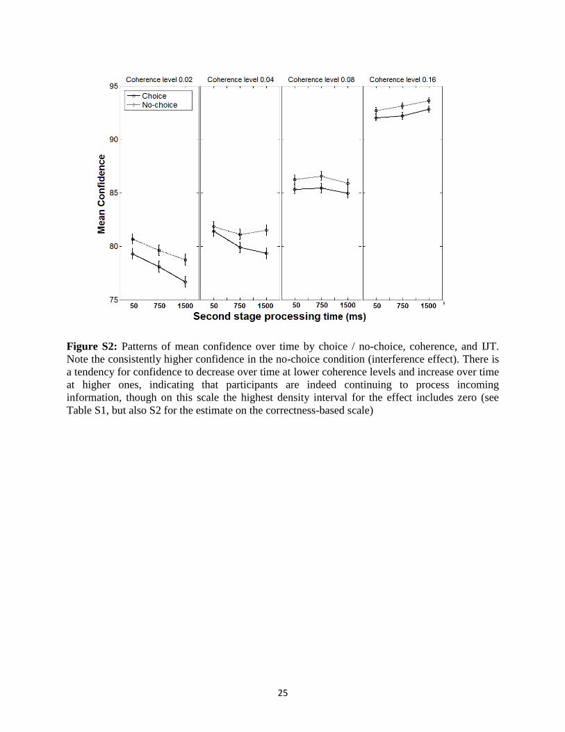
25
Figure S2: Patterns of mean confidence over time by choice / no-choice, coherence, and IJT.
Note the consistently higher confidence in the no-choice condition (interference effect). There is
a tendency for confidence to decrease over time at lower coherence levels and increase over time
at higher ones, indicating that participants are indeed continuing to process incoming
information, though on this scale the highest density interval for the effect includes zero (see
Table S1, but also S2 for the estimate on the correctness-based scale)

26
Figure S3: Outline of the dynamics of each model when a rightward moving stimulus is
presented. Panels plot hypothetical probability distributions at different time points over different
evidence levels, with levels 0–50 corresponding to states that favor the ‘left’ incorrect response
and levels 50–100 corresponding to those that favor the ‘right’ correct response. Note that in this
depiction we assume only 101 rather than 103 states. Each model has an initial state – a mixed
state vector in the Markov model, or a superposition state vector in the quantum model – which
is centered over 50, indicating uncertainty (A, B). Each one uses a drift (δ) and diffusion (σ2)

27
parameter to describe the average rate of correct evidence and noise accumulated, respectively
(C, D), but constructs the operator differently. At t1, if no choice is cued, then the dynamics
continue to be applied. However, if at t1 a choice is cued, a decision is read out from the MRW,
with ‘right’ being chosen if the evidence is above the decision criterion (E). In the QRW, the
probability of choosing ‘left’ or ‘right’ is determined by the sum of the squared potentials over
those states (F). Moreover, in the QRW, a choice requires that the state be projected onto the
corresponding bases (e.g., 50–100 if ‘right’ is correctly chosen), eliminating the potentials over
the states less than 50 and producing a change in the cognitive state. This projection, along with
the dynamics applied from t1 to t2 (G, H), results in a different distribution of confidence for the
choice and no-choice conditions in the QRW (K). However, because no change is made to the
state at t1 due to choice in the MRW, this model predicts that the distributions will be the same
for choice and no-choice conditions (J). We present the formal mathematical construction of
each model in the main text of the paper, and proofs are supplied in Appendix C.

28
Figure S4: Data along with maximum-likelihood predictions from the Markov and quantum
random walk models. Shown are the marginal probability density of confidence responses
choice condition and the no-choice condition (top 2 panels for each participant) collapsed across
second-stage processing and dot motion coherence manipulations. Also shown are the observed
and maximum likelihood predictions for choice proportions in each dot motion coherence
condition (bottom panel of each participant). Note that some participants tended to group their
responses (e.g. participant #7 used 0/10/20/etc.) – further work incorporating individual
differences in response mapping would certainly improve fits for both models, but response
mapping does not directly affect interference (see proof in Appendix C).
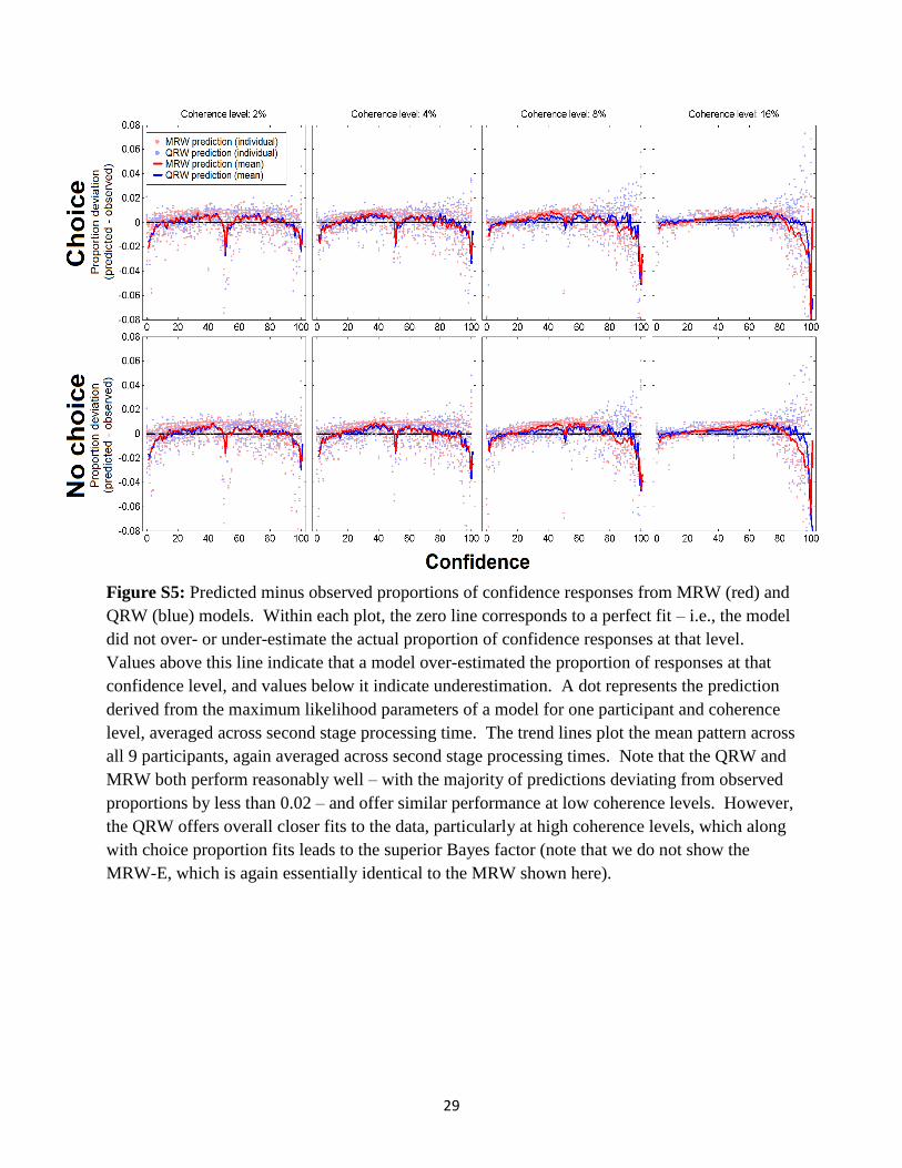
29
Figure S5: Predicted minus observed proportions of confidence responses from MRW (red) and
QRW (blue) models. Within each plot, the zero line corresponds to a perfect fit – i.e., the model
did not over- or under-estimate the actual proportion of confidence responses at that level.
Values above this line indicate that a model over-estimated the proportion of responses at that
confidence level, and values below it indicate underestimation. A dot represents the prediction
derived from the maximum likelihood parameters of a model for one participant and coherence
level, averaged across second stage processing time. The trend lines plot the mean pattern across
all 9 participants, again averaged across second stage processing times. Note that the QRW and
MRW both perform reasonably well – with the majority of predictions deviating from observed
proportions by less than 0.02 – and offer similar performance at low coherence levels. However,
the QRW offers overall closer fits to the data, particularly at high coherence levels, which along
with choice proportion fits leads to the superior Bayes factor (note that we do not show the
MRW-E, which is again essentially identical to the MRW shown here).

30
Figure S6: Cumulative distributions of confidence responses in the data (black) and maximum
likelihood predictions from the QRW (blue) and MRW (red) for choice and no-choice
conditions, averaged across participants, coherence levels, and second stage processing times.
There are four things to note: 1) the difference between choice and no-choice conditions in the
data (interference effect); 2) a similar effect in the QRW, showing its ability to predict
interference; 3) the lack of difference between choice and no-choice in the MRW (no
interference); and 4) the closer fit of the QRW to the data relative to the MRW.
However, it is critical to note that the cumulative distribution provides a misleading depiction of
the fit of the models, as the deviation between curves shows the accumulated error across many
confidence levels. The errors at individual confidence levels are comparatively quite small – a
much more accurate impression of fit can be gathered from the probability mass distributions
shown in Figures 3 and S4 as well as the deviations in probability mass shown in Figure S5.
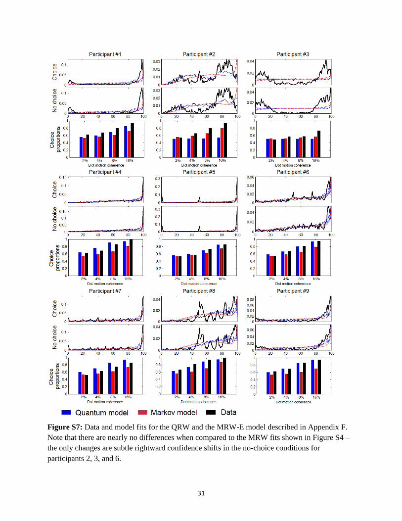
31
Figure S7: Data and model fits for the QRW and the MRW-E model described in Appendix F.
Note that there are nearly no differences when compared to the MRW fits shown in Figure S4 –
the only changes are subtle rightward confidence shifts in the no-choice conditions for
participants 2, 3, and 6.

32
Tables
Factor Mean 95% HDI
Second-stage processing
time (SPT) -0.05 [-0.10 0.00]
Coherence 0.50 [0.04 1.16]
Choice / No-choice (C/N) -0.11 [-0.18 -0.04]
SPT × C/N -0.02 [-0.08 0.04]
Coherence × SPT 0.05 [-0.01 0.12]
Coherence × C/N 0.04 [-0.04 0.12]
Coherence × SPT × C/N 0.00 [-0.08 0.08]
Table S1: Main effects and interactions of dot coherence, second-stage processing time (SPT),
and the choice / no-choice manipulation (C/N) predicting confidence on the half scale (50-100).
Note that the interaction between coherence and SPT is not significant on the half scale, as more
evidence for the true state of the world (higher coherence) will increase confidence over time for
correct estimates but decrease confidence over time for incorrect ones, and these conflicting
patterns wash or cancel each other out
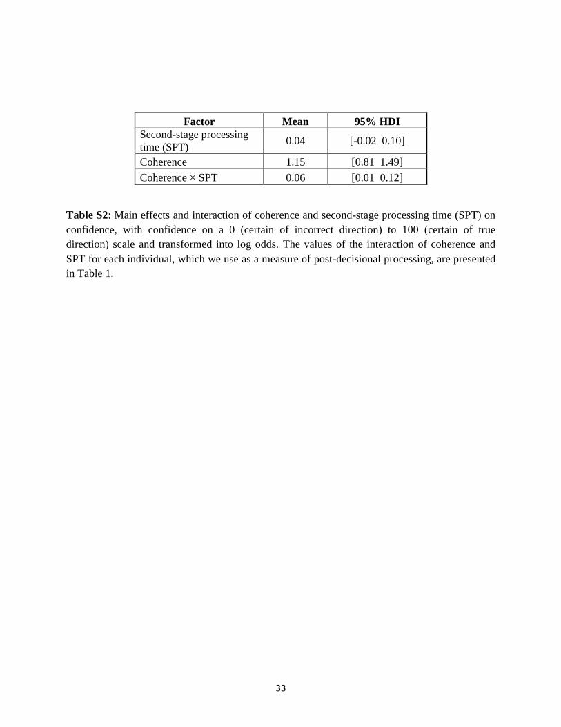
33
Factor Mean 95% HDI
Second-stage processing
time (SPT) 0.04 [-0.02 0.10]
Coherence 1.15 [0.81 1.49]
Coherence × SPT 0.06 [0.01 0.12]
Table S2: Main effects and interaction of coherence and second-stage processing time (SPT) on
confidence, with confidence on a 0 (certain of incorrect direction) to 100 (certain of true
direction) scale and transformed into log odds. The values of the interaction of coherence and
SPT for each individual, which we use as a measure of post-decisional processing, are presented
in Table 1.
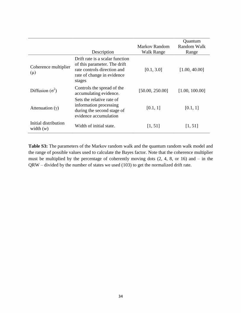
34
Description
Markov Random
Walk Range
Quantum
Random Walk
Range
Coherence multiplier
(μ)
Drift rate is a scalar function
of this parameter. The drift
rate controls direction and
rate of change in evidence
stages
[0.1, 3.0] [1.00, 40.00]
Diffusion (σ2)
Controls the spread of the
accumulating evidence. [50.00, 250.00] [1.00, 100.00]
Attenuation ()
Sets the relative rate of
information processing
during the second stage of
evidence accumulation
[0.1, 1] [0.1, 1]
Initial distribution
width (w) Width of initial state. [1, 51] [1, 51]
Table S3: The parameters of the Markov random walk and the quantum random walk model and
the range of possible values used to calculate the Bayes factor. Note that the coherence multiplier
must be multiplied by the percentage of coherently moving dots (2, 4, 8, or 16) and – in the
QRW – divided by the number of states we used (103) to get the normalized drift rate.

35
Model
Participant QRW MRW
1 -14521 -14734
2 -11692 -11725
3 -14932 -14801
4 -11586 -11777
5 -10908 -11747
6 -12358 -12581
7 -12031 -11882
8 -12034 -12373
9 -14424 -14574
Table S4: Maximum log likelihood for each model and participant resulting from the grid search
used to compute the Bayes factor. Note that the Bayes factor reflects closely the difference
between log likelihoods – maximum likelihood estimates tended to be much better than next-best
estimates simply due to the large number of data points, giving the priors little influence over the
posterior odds.

36
Participant Model Coherence
Multiplier (μ) Diffusion (σ²) Width (w)
Attenuation
(γ)
1
MRW 2.71 220 51 1
QRW 24.4 55.45 1 0.235
2
MRW 2.57 230 34 0.415
QRW 1.00 95.05 48 0.865
3
MRW 0.68 230 51 1
QRW 1.00 1 51 1
4
MRW 3.00 130 39 0.685
QRW 23.46 60.4 3 0.1
5
MRW 2.71 240 51 1
QRW 24.45 55.45 1 0.19
6
MRW 2.86 250 39 0.595
QRW 22.50 55.45 2 0.235
7
MRW 3.00 250 51 0.865
QRW 28.30 60.4 2 0.1
8
MRW 2.86 230 28 0.505
QRW 18.55 65.35 4 0.235
9
MRW 2.57 220 51 1
QRW 28.30 60.4 2 0.1
Table S5: Maximum likelihood parameter estimates for each participant and model, obtained
from the grid search. Note that in most cases, the maximum likelihood estimates were far
superior to most other estimates, so we do not include posterior probability density intervals.
Also, recall that the coherence multiplier must be multiplied by the percentage of coherently
moving dots (2, 4, 8, or 16) and number of states in the QRW (103) to get the drift rate.
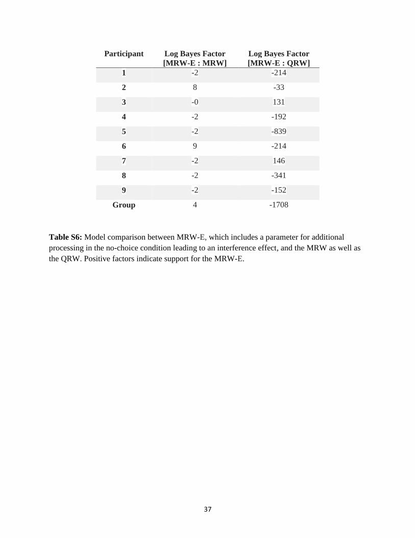
37
Participant Log Bayes Factor
[MRW-E : MRW]
Log Bayes Factor
[MRW-E : QRW]
1 -2 -214
2 8 -33
3 -0 131
4 -2 -192
5 -2 -839
6 9 -214
7 -2 146
8 -2 -341
9 -2 -152
Group 4 -1708
Table S6: Model comparison between MRW-E, which includes a parameter for additional
processing in the no-choice condition leading to an interference effect, and the MRW as well as
the QRW. Positive factors indicate support for the MRW-E.
Recommended