ORNL/TM-2015/14
Hydropower Baseline Cost Modeling
January 2015
Prepared by
Patrick W. O’Connor
Qin Fen (Katherine) Zhang
Scott T. DeNeale
Dol Raj Chalise
Emma Centurion
Approved for public release;
distribution is unlimited.
DOCUMENT AVAILABILITY
Reports produced after January 1, 1996, are generally available free via the U.S. Department of
Energy (DOE) Information Bridge.
Web site http://www.osti.gov/bridge
Reports produced before January 1, 1996, may be purchased by members of the public from the
following source.
National Technical Information Service
5285 Port Royal Road
Springfield, VA 22161
Telephone 703-605-6000 (1-800-553-6847)
TDD 703-487-4639
Fax 703-605-6900
E-mail [email protected]
Web site http://www.ntis.gov/support/ordernowabout.htm
Reports are available to DOE employees, DOE contractors, Energy Technology Data Exchange
(ETDE) representatives, and International Nuclear Information System (INIS) representatives from
the following source.
Office of Scientific and Technical Information
P.O. Box 62
Oak Ridge, TN 37831
Telephone 865-576-8401
Fax 865-576-5728
E-mail [email protected]
Web site http://www.osti.gov/contact.html
This report was prepared as an account of work sponsored by an
agency of the United States Government. Neither the United States
Government nor any agency thereof, nor any of their employees,
makes any warranty, express or implied, or assumes any legal
liability or responsibility for the accuracy, completeness, or
usefulness of any information, apparatus, product, or process
disclosed, or represents that its use would not infringe privately
owned rights. Reference herein to any specific commercial product,
process, or service by trade name, trademark, manufacturer, or
otherwise, does not necessarily constitute or imply its endorsement,
recommendation, or favoring by the United States Government or
any agency thereof. The views and opinions of authors expressed
herein do not necessarily state or reflect those of the United States
Government or any agency thereof.
ORNL/TM-
Hydropower Baseline Cost Modeling
Date Published: January 2015
Prepared by
OAK RIDGE NATIONAL LABORATORY
Oak Ridge, Tennessee 37831-6283
managed by
UT-BATTELLE, LLC
for the
U.S. DEPARTMENT OF ENERGY
under contract DE-AC05-00OR22725

(THIS PAGE LEFT BLANK INTENTIONALLY)
iii
Table of Contents
Executive Summary ................................................................................................................................. vii
1. Introduction ........................................................................................................................................... 1
1.1. Background ..................................................................................................................................... 1
2. Data Collection ..................................................................................................................................... 3
2.1. Framework ....................................................................................................................................... 3
2.2. Data Sources .................................................................................................................................. 6
2.3. Cost Escalation ............................................................................................................................. 10
2.4. Discussion ..................................................................................................................................... 12
3. Analysis Methodology ....................................................................................................................... 18
3.1. Model Development ..................................................................................................................... 18
3.2. Model Selection and Evaluation ................................................................................................. 19
4. Model Results ..................................................................................................................................... 22
4.1. Non-powered Dams (NPDs) ....................................................................................................... 22
4.2. New Stream-reach Development (NSDs) ................................................................................ 28
4.3. Canal/Conduits ............................................................................................................................. 34
4.4. Pumped Storage Hydropower (PSH) ........................................................................................ 39
4.5. Unit Addition .................................................................................................................................. 42
4.6. Generator Rewind ........................................................................................................................ 43
4.7. Results Summary, Discussion, and Application ...................................................................... 44
5. Conclusions and Future Work ......................................................................................................... 46
References ................................................................................................................................................ 48
Appendix A – Alternative Models, Detailed Comparison, and Validation ...................................... A-1

iv
List of Figures
Figure 1. Hydropower Cost Breakdown Structure ................................................................................ 4 Figure 2. Project activity diagram for IIR database (Cotchen, 2014) ................................................. 6 Figure 3. Cost indexes comparison ....................................................................................................... 12 Figure 4. Finalized BCM data project count by data source, project development stage, and resource category..................................................................................................................................... 13 Figure 5 - Capital costs of recently developed hydropower facilities ............................................... 15 Figure 6 - Levelized Cost of Energy (LCOE) of recently developed new hydropower resources 16 Figure 7. NPD data distribution histograms ......................................................................................... 24 Figure 8. NPD project raw data scatter plots ....................................................................................... 25 Figure 9. Comparison of ORNL and INL model-estimated costs with actual NPD costs ... 27 Figure 10. Breakdown cost distribution for NPD projects (EC dataset) ........................................... 28 Figure 11. NSD project raw data distribution histograms................................................................... 30 Figure 12. NSD project raw data scatter plots ..................................................................................... 31 Figure 13. Comparison of ORNL and INL model-estimated costs with actual NSD costs ........... 33 Figure 14. Breakdown cost distribution for NSD projects (EC dataset) ........................................... 34 Figure 15. Canal/Conduit project raw data distribution histograms .................................................. 36 Figure 16. Canal/Conduit project raw data scatter plots .................................................................... 37 Figure 17. Breakdown cost distribution for Canal/Conduit projects (EC dataset) .......................... 38 Figure 18. PSH project raw data distribution histograms ................................................................... 40 Figure 19. PSH project raw data scatter plots ..................................................................................... 41 Figure 20. Breakdown cost distribution for PSH projects (PE dataset) ........................................... 42 Figure 21 - Application of NSD and NPD BCMs to U.S. undeveloped resources > 1 MW ........... 45 Figure 22. Raw data statistics .............................................................................................................. A-3 Figure 23. Regional classification of the United States .................................................................... A-4 Figure 24. Regional distribution of Non Powered Dams (NPDs) cost data ................................... A-7 Figure 25. NPD in-sample model validation ....................................................................................... A-9 Figure 26. NPD breakdown cost distributions by Capacity range ................................................ A-10 Figure 27. NPD breakdown cost distributions by Head range ...................................................... A-11 Figure 28. Regional distribution of New Stream-reach Development (NSDs) cost data .......... A-14 Figure 29. NSD in-sample model validation ..................................................................................... A-16 Figure 30. NSD breakdown cost distributions by Capacity range ................................................ A-17 Figure 31. NSD breakdown cost distributions by Head range ...................................................... A-18 Figure 32. Regional distribution of Canal/Conduit cost data ......................................................... A-20 Figure 33. Canal/Conduit in-sample model validation .................................................................... A-22 Figure 34. Canal/Conduit breakdown cost distributions by Capacity range ............................... A-23 Figure 35. Canal/Conduit breakdown cost distributions by Head range ..................................... A-24 Figure 36. Regional distribution of PSH cost data .......................................................................... A-26 Figure 37. PSH in-sample model validation ..................................................................................... A-28 Figure 38. PSH breakdown cost distributions by Capacity range ................................................. A-29 Figure 39. PSH breakdown cost distributions by Head range ....................................................... A-29 Figure 40. Regional distribution of Unit Addition cost data ............................................................ A-31 Figure 41. Regional distribution of Generator Rewind cost data .................................................. A-32 Figure 42. Unit Addition and Generator Rewind in-sample model validation ............................. A-34 Figure 43. Unit Addition and Generator Rewind in-sample model validation ............................. A-34

v
vi
List of Tables
Table 1. Summary of projects collected from FERC............................................................................. 7
Table 2. Summary of projects collected from the DOE-EPRI small-hydropower development
report ............................................................................................................................................................ 8
Table 3. Summary of projects collected from the IIR database .......................................................... 9
Table 4. Summary of Other data sources ............................................................................................ 10
Table 5. Summary of projects collected from Other sources ............................................................ 10
Table 6 - Summary of projects with actual costs (C-stage) ............................................................... 13
Table 7. Comparison between planning, engineering, and construction stage cost for DOE-EPRI
dataset projects ........................................................................................................................................ 17
Table 8. Comparison between actual project cost, engineering stage, and feasibility stage cost
for IIR dataset ........................................................................................................................................... 17
Table 9. Confidence Score Criteria ....................................................................................................... 21
Table 10. NPD Project Summary Statistics .......................................................................................... 23
Table 11. NPD recommended model summary .................................................................................. 25
Table 12. NSD project summary statistics ........................................................................................... 29
Table 13. NSD recommended model summary .................................................................................. 31
Table 14. Canal/Conduit project summary statistics .......................................................................... 35
Table 15. Canal/Conduit recommended model summary ................................................................. 38
Table 16. PSH project summary statistics ............................................................................................ 39
Table 17. PSH recommended model summary .................................................................................. 41
Table 18. Unit Addition recommended model summary .................................................................... 43
Table 19. Generator Rewind recommended model summary .......................................................... 43
Table 20. Baseline cost model results by resource category ............................................................ 44
Table 21. Summary regression results for NPDs .............................................................................. A-8
Table 22. Summary regression results for NSDs ............................................................................ A-15
Table 23. Summary regression results for Canal/Conduit ............................................................. A-21
Table 24. Summary regression results for PSH .............................................................................. A-27
Table 25. Summary regression results for Unit Addition and Generator Rewind ...................... A-33
vii
Executive Summary
Recent resource assessments conducted by the United States Department of Energy have
identified significant opportunities for expanding hydropower generation through the addition of
power to non-powered dams and on undeveloped stream-reaches. Additional interest exists in
the powering of existing water resource infrastructure such as conduits and canals, upgrading
and expanding existing hydropower facilities, and the construction new pumped storage
hydropower. Understanding the potential future role of these hydropower resources in the
nation’s energy system requires an assessment of the environmental and techno-economic
issues associated with expanding hydropower generation. To facilitate these assessments, this
report seeks to fill the current gaps in publically available hydropower cost-estimating tools that
can support the national-scale evaluation of hydropower resources.
The report presents the background, framework, methodology, and results of the collection of
contemporary cost data and the development of a series of parametric models to predict the
initial capital cost (ICC) of hydropower projects. Recent cost data helps provide the economic
context for recent hydropower development; the parametric “baseline cost models” are used to
generate cost estimates for hydropower projects in various resource categories and are
intended to produce generalized, representative estimates suitable for the national or regional-
scale evaluation of hydropower economic competitiveness. More sophisticated, bottom-up (as
opposed to top-down, parametric) techniques are necessary for the development of individual
site costs; however, the parametric approaches described in the report are a necessary
simplification to systematically evaluate hydropower potential across the U.S.
Nearly 600 unique cost estimates were gathered from 16 different sources, including reports,
market intelligence databases, and private communications with owners, developers and
consultants. The scope and extent of each cost estimate varied with many projects lacking data
for the costs and risks associated with the licensing, permitting, and development of hydropower
projects. Future iterations of this report will tackle the contemporary costs of the licensing and
project development processes, but in this initial iteration, references to historical estimates of
the cost of licensing hydropower projects are provided within the report.
Based on the United States-only subset of the collected data, the cost of constructing a
hydropower plant on existing conduits, on non-powered dams, or along new, undeveloped
stream reaches has ranged from $1000 to $9000 per kilowatt, with the average canal project
averaging $4100 per kilowatt, the average non-powered dam project costing approximately
$3800 per kilowatt and development along new stream reaches costing approximately $4900
per kilowatt. In all three cases costs were most noticeably driven by economies of scale (i.e.
lower costs) from higher hydraulic head, while only canal projects exhibited meaningful
economies of scale from higher installed capacity. Across the timespan of the collected data
(roughly 1980 to present), construction costs for hydropower plants have not grown on a real,
inflation adjusted basis. On a lifecycle basis, for those plants for which generation estimates
were available, the unsubsidized levelized cost of energy (LCOE) of constructing recent
hydropower plants has ranged from $30 to $180 per megawatt-hour, with the median project
viii
costing approximately $110 per megawatt-hour (excluding licensing) for powering conduits, non-
powered dams, and new stream reaches.
In addition to the construction of power generating facilities on previously unpowered
infrastructure or stream reaches, costs estimates were also collected for the installation of
additional units in existing powerhouses and the rewinding of existing generators; the average
addition of a new unit to an existing powerhouse has cost $1930 per kilowatt, and the average
generator rewind has cost $114 per kilowatt, but both are subject to strong economies of scale
based on the size of the units involved.
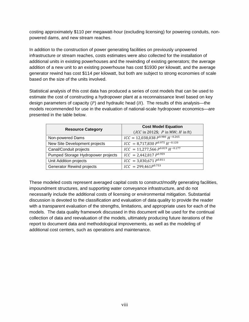
Statistical analysis of this cost data has produced a series of cost models that can be used to
estimate the cost of constructing a hydropower plant at a reconnaissance level based on key
design parameters of capacity (𝑃) and hydraulic head (𝐻). The results of this analysis—the
models recommended for use in the evaluation of national-scale hydropower economics—are
presented in the table below.
Resource Category Cost Model Equation
(ICC in 2012$; P in MW; H in ft)
Non-powered Dams 𝐼𝐶𝐶 = 12,038,038 𝑃0.980 𝐻−0.265
New Site Development projects 𝐼𝐶𝐶 = 8,717,830 𝑃0.975 𝐻−0.120
Canal/Conduit projects 𝐼𝐶𝐶 = 11,277,566 𝑃0.819 𝐻−0.177
Pumped Storage Hydropower projects 𝐼𝐶𝐶 = 2,442,817 𝑃0.959
Unit Addition projects 𝐼𝐶𝐶 = 3,030,671 𝑃0.811
Generator Rewind projects 𝐼𝐶𝐶 = 299,461𝑃0.753
These modeled costs represent averaged capital costs to construct/modify generating facilities,
impoundment structures, and supporting water conveyance infrastructure, and do not
necessarily include the additional costs of licensing or environmental mitigation. Substantial
discussion is devoted to the classification and evaluation of data quality to provide the reader
with a transparent evaluation of the strengths, limitations, and appropriate uses for each of the
models. The data quality framework discussed in this document will be used for the continual
collection of data and reevaluation of the models, ultimately producing future iterations of the
report to document data and methodological improvements, as well as the modeling of
additional cost centers, such as operations and maintenance.
1
1. Introduction
1.1. Background
Recently, the United States (U.S.) Department of Energy (DOE) completed major assessments
to identify hydropower resource development potential nationwide. In 2012, researchers from
Idaho National Laboratory (INL) and Oak Ridge National Laboratory (ORNL) completed the
Non-Powered Dam (NPD) Resource Assessment (Hadjerioua et al., 2012) which indicated the
potential to expand hydropower by up to 12.1 GW at NPDs across the U.S. In a similar fashion,
in 2014, researchers at ORNL completed the New Stream-reach Development (NSD) Resource
Assessment (Kao et al., 2014) and identified over 65 GW of additional undeveloped hydropower
potential. Compared with the current U.S. hydropower fleet totaling approximately 80 GW,
these reports demonstrate significant expansion potential exists. Additionally, substantial
interest also exists in the powering of other existing water resource infrastructure such as canals
and conduits, and the use of Pumped Storage Hydropower to balance an increasingly
renewable grid. While the resource potential for new hydropower is clear, improved costing
tools are necessary to evaluate the economic feasibility of these resources.
Comprehensive engineering design and cost evaluations would provide the most accurate site-
specific cost estimates, however data limitations and the breadth of hydropower sites across the
U.S. makes the systematic use of such costing methods infeasible for evaluating national-scale
economic competitiveness and resource potential. Statistical and parametric cost estimation
provides a simpler alternative method for evaluating the cost dynamics of hydropower resources
at a national scale. While previous studies have been conducted to evaluate U.S. hydropower
development costing, the existing models suffer from several issues including that:
the most recent DOE-sponsored comprehensive cost study was conducted over 10
years ago (INL, 2003);
many existing cost models are largely outdated or bas on non-U.S. data;
key resource classes, particularly NPDs and canal/conduit projects are not explicitly
modeled; and
the existing models may lack appropriate detail to accurately cost the generally smaller,
lower head resources identified in recent resource assessments (Zhang et al., 2012).
To address these existing gaps in the publically available literature on hydropower costing,
better assess the viability of developing these significant untapped resources, and help identify
key areas for research, development, and deployment (RD&D), ORNL has developed a series
of Baseline Cost Models (BCMs) and associated tools for estimating the initial capital cost (ICC)
of developing hydropower in the U.S. based on historical project data.
2
The primary objective is to develop tools which generate cost estimates that accurately reflect
the economics of hydropower at a national scale. Examples of targeted end-uses include
transparent comparisons of the cost and performance of electricity generating technologies
(OpenEI, 2014 and EIA, 2013), long-term forecasting such as annual projections by the U.S.
Energy Information Administration (EIA, 2014b), and strategic planning and technology potential
evaluations by the U.S. Department of Energy (DOE), such as the recent Sunshot Vision (DOE,
2012) and Renewable Electricity Futures (NREL, 2012) studies.
Aside from DOE, the cost estimating tools can provide value to multiple other users such as
utilities conducting resource planning studies that would benefit from contemporary hydropower
cost estimates. While new costing tools may also be useful for high-level cost estimation for
screening-level assessments, it is important to note that the site-specificity inherent in
hydropower development limits the applicability for individual project feasibility.
To support these objects, this report documents the processes involved in collecting,
processing, and analyzing the raw data to produce hydropower cost estimation models for six
specific categories of hydropower projects. The first four categories are the addition of new
hydropower resources where no powerhouse currently exists, including:
1. Non-powered Dams (NPD) – Encompassing the construction of a new
powerhouse at existing dams or other facilities. This category of model may also be
useful for estimating the costs of adding a powerhouse to an existing powered dam.
2. New Stream-reach Development (NSD) projects – Greenfield projects with no
existing facilities.
3. Canal/Conduit projects – Involves power development at existing Canals or
Conduits.
4. Pumped Storage Hydropower (PSH) projects –Connects an upper and lower
reservoir via a pump-turbine arrangement to provide energy generation as well as
pumping power for maintaining storage availability.
The last two cost estimating tools are derived to project the cost of modifying existing
powerhouses—they cover only two specific types of modification:
5. Unit Addition projects – Involves existing plant renovation or expansion. The
project should clearly involve a change in installed capacity. This type of project
may include acquisition and installation of a new turbine-generator unit but
excludes construction of a new powerhouse.
6. Generator Rewind projects – Generator refurbishment to improve efficiency and
extend unit service life.
There are many other categories of improvement projects for the existing hydropower fleet,
however, data limitations prevented the development of reliable models for this iteration of the
BCM report.
To quantify the contemporary cost of developing resources and document model development,
the data collection framework and sources used in this report are introduced and discussed in
3
Section 2, while Section 3 details the generalized model development and evaluation
framework. Section 4 presents the recommended BCM for each resource class, with additional
validation and model alternatives are provided in Appendix A. The recommended models for
NPD and NSD are also applied to recent DOE resource assessments to illustrate the national
scale distribution of hydropower costs.
Ultimately, this report is intended to serve as a living document incrementally updated as
continued DOE efforts to capture additional cost data and develop improved modeling
techniques result in increasingly useful costing tools for the research community and
hydropower industry.
2. Data Collection
2.1. Framework
The acquisition and validation of quality cost data is the foundation of any modeling exercise. In
the development of the BCM, significant attention was paid to two key determinants of data
quality: the scope of the cost estimate and the certainty of the estimate with respect to what
would be expected from a finalized, constructed project.
Cost Scope
The cost of hydropower development can be broken down into variety of distinct components
ranging from the substantial effort required to permit and design the plant, to the extensive
construction and civil works and the acquisition and installation of generating equipment.
Accurate comparisons and analyses of cost must necessarily draw clear distinctions on the
scope of which the utilized cost estimates include and exclude.
To facilitate the systematic application of clear boundaries on collected cost data, a Cost
Breakdown Structure (CBS) was developed that partitions the components of hydropower
capital costs into a clear hierarchy. At the highest level (1) of this hierarchy is the Initial Capital
Cost (ICC) representing the full capital outlay necessary for a hydropower plant to reach
commercial operation. ICC is further divided into three subcomponents at level 2: The
Generating Plant (all physical components directly necessary for power generation), Balance of
Station (all development expenditures and additional costs, such as those required to meet
environmental and regulatory requirements, or the construction of substations and transmission
lines), and Financial Costs (the highly variable costs of obtaining and repaying the capital used
in developing and constructing a hydropower project). The CBS is graphically depicted at level
3 in Figure 1.

4
Figure 1. Hydropower Cost Breakdown Structure
1 Initial Capital Costs (ICC)
1.1 Generating Plant
1.1.1 Site Preparation
1.1.2 Dams and Reservoirs
1.1.3 Water Conveyance
1.1.4 Powerhouse Structures
1.1.5 Powertrain Equipment
1.1.6 Ancillary Electrical
Equipment
1.1.7 Ancillary Mechanical Equipment
1.2 Balance of Station
1.2.1 Development
1.2.2 Engineering and Management
1.2.3 Electrical Infrastructure
1.2.4 Plant Commissioning
1.2.5 Site Access
1.2.6 Operation and Maintenance
Infrastructure
1.2.7 Env. Mitigation and
Regulatory Compliance
1.2.8 Navigation Locks
1.3 Financial Costs
1.3.1 Project Contingency
1.3.2 Construction Insurance
1.3.3 Carrying Charges during
Construction
1.3.4 Reserve Accounts
1.3.5 Uncategorized
Project Overruns
Civ
il W
ork
s
Eq
uip
men
t

5
Figure 1 draws an additional distinction within the Generating Plant components between (a)
site preparation and construction intensive structures (“Civil Works”) and (b) the equipment
portion of plant expenditures (“Electro-Mechanical Equipment” or “Equipment”) as the sourcing
and composition of these costs are distinct from one another. Generating plant breakdown costs
are presented in these categories in Section 4 and Appendix A of the document to efficiently
visualize cost distribution without overwhelming detail.
Cost Certainty
Understanding the source, rigor, and detail of an estimate can give a perspective on its certainty
or accuracy. As an example. major cost engineering professional associations categorize
project costs into distinct estimate stages based on project maturity and estimate end use (see
AACE, 2013), assigning quantitative cost uncertainty to each stage. Ideally a similar quantitative
system could be applied to the BCM to provide a mechanism for assessing the certainty and
accuracy of collected data. However, in the development of the BCM, data has been collected
from a variety of different sources (described in detail in Section 2.2), and access to the project
development information necessary to place the project directly onto such a scale was typically
unavailable. While this prevented the direct application of quantitative certainty to the data, it
was still determined that capturing data on the stage of project development could provide
useful modeling distinctions. To capture project development in a limited information
environment, a simplified categorization system was adapted from an existing system in use by
one of the BCM’s primary data sources, Industrial Information Resources (IIR). IIR is introduced
in more detail in Section 2.2, but its categorization system is described here to provide context
for its use throughout the report.
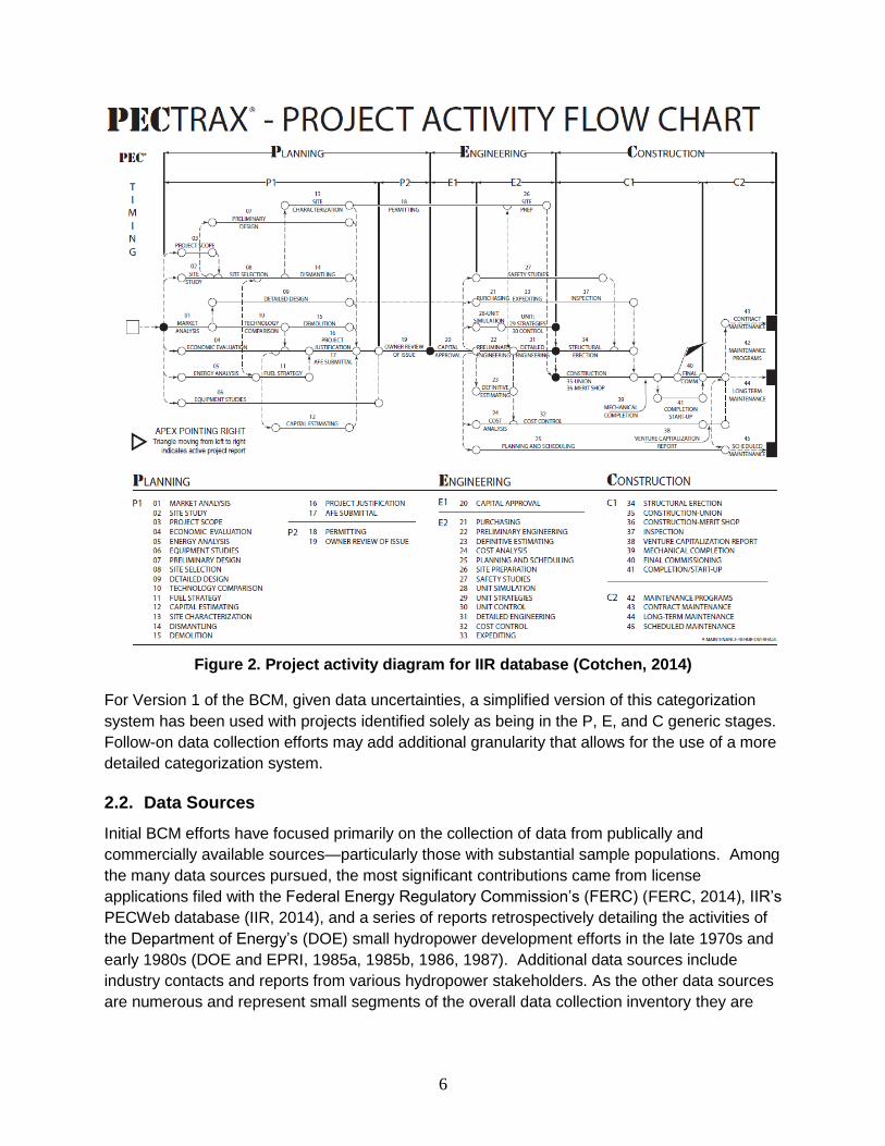
IIR uses alphanumeric categories in the broad groups of Planning (P), Engineering (E), and
Construction (C). The definition of each stage within this “PEC” system is shown in Figure 2
(Cotchen, 2014). As shown in the IIR project activity diagram, P1 is a preliminary project activity
and an initial step in the planning stage before starting a project. P1 includes site selection as
well as preliminary design and economic analysis. P2 is the final step in the planning stage and
mainly focuses on licensing activity for the project. After obtaining the project license, E1
represents an initial step in the engineering stage associated with the capital approval process.
E2 is the final step in the engineering stage and typically includes detailed engineering design
and cost estimation, planning, scheduling, and site preparation. C1 is the first step in the
construction stage and includes all site construction activities until final commissioning of a
project. C2 is the final step in the project activity chart and represents project completion with
associated post-construction maintenance activities. Although hydropower costs are highly site-
specific with many factors contributing to cost uncertainty, cost accuracy is generally assumed
to increase as project development nears completion. As such, construction stage cost
estimates are necessarily considered the most accurate (and are quantitatively defined as such
by AACE).
6
Figure 2. Project activity diagram for IIR database (Cotchen, 2014)
For Version 1 of the BCM, given data uncertainties, a simplified version of this categorization
system has been used with projects identified solely as being in the P, E, and C generic stages.
Follow-on data collection efforts may add additional granularity that allows for the use of a more
detailed categorization system.
2.2. Data Sources
Initial BCM efforts have focused primarily on the collection of data from publically and
commercially available sources—particularly those with substantial sample populations. Among
the many data sources pursued, the most significant contributions came from license
applications filed with the Federal Energy Regulatory Commission’s (FERC) (FERC, 2014), IIR’s
PECWeb database (IIR, 2014), and a series of reports retrospectively detailing the activities of
the Department of Energy’s (DOE) small hydropower development efforts in the late 1970s and
early 1980s (DOE and EPRI, 1985a, 1985b, 1986, 1987). Additional data sources include
industry contacts and reports from various hydropower stakeholders. As the other data sources
are numerous and represent small segments of the overall data collection inventory they are

7
introduced briefly at the end of this section while more detailed description is provided for the
FERC, IIR, and DOE sources.
Federal Energy Regulatory Commission (FERC) Application Documents
FERC issues preliminary permits, licenses, and relicenses (or in some cases grants
exemptions) for the vast majority of non-federal hydropower projects. In applications for original
or new licenses, most major projects above 5 MW are required to submit actual or approximate
original cost1. Major water projects whose installed capacity is less than 5 MW and minor water
projects of less than 1.5 MW must include the estimated cost of the project and of each
proposed environmental mitigation measure2. Some of the license application files containing
cost information are not publicly available, and many of the licenses submitted before 2007
cannot be accessed. Preliminary permits typically do not include useful cost information, but
may at times provide cost estimates for the studies to be performed before applying for a full
license.
The license, preliminary permit, and exemption application documents are available through
FERC’s eLibrary regulatory document database.3 Documents submitted for preliminary permits,
and to a lesser extent full license applications, are based on early cost estimates, and the
corresponding cost accuracy will typically be low. So, in order to classify these FERC projects
on the simplified PEC scale, those license applications with breakdown (component) cost
estimates were classified as engineering (E) stage, while permit applications and license
applications lacking component-level detail were classified as planning stage projects (P). The
total number of projects collected from FERC are shown in Table 1 based on hydro resource
category and project development stage.
Table 1. Summary of projects collected from FERC
Resource Category
Project Count
Development Stage (count)
Capacity (MW) Head (ft) No. of
Projects with
Breakdown Cost
P E C Min Avg Max Min Avg Max
NSD 8 2 6 0 0.4 51.71 121.5 57 376 966 6
NPD 26 5 21 0 0.205 12.84 48 13 98 700 21
Canal 9 4 5 0 0.225 1.72 6.15 34 211 445 5
PSH 7 0 7 0 280 868.6 1,300 720 1,324 1,866 3
DOE National Small Hydropower Program
In 1977, the DOE launched the National Small-Hydropower Program to promote the
development of smaller, lower-impact hydropower. As a part of this program, DOE sponsored a
number of small hydro projects at feasibility study, licensing, or construction stages, later joining
with the Electric Power Research Institute (EPRI) to collect, organize, analyze, and summarize
the results. During 1985-1987, the DOE and EPRI jointly published and made publicly available
1 This information is found in a License application’s “Exhibit D” and/or “Exhibit A”
2 This information is found in a License application’s “Exhibit A”
3 To access the FERC e-Library, visit http://www.ferc.gov/docs-filing/elibrary.asp.

8
“Small-Hydropower Development: The Process, Pitfalls, and Experience,” a four-volume report
documenting the scope and results of the collaboration with the goal of benefitting future
hydropower development initiatives (DOE and EPRI, 1985a, 1985b, 1986, 1987).
Volume 1 of the DOE-EPRI report presents 240 feasibility studies and summarizes individual
project information such as location, ownership, and hydrological and hydraulic features, as well
as details related to the generating equipment, transmission, capital cost, and environmental
and economic analyses performed (DOE and EPRI, 1985a). Volume 2 describes 41 projects
which entered the licensing process and provides additional information related to licensing
activities and enhanced project scope (DOE and EPRI, 1985b). The third Volume provides
details on 23 projects, 17 which had completed construction and 6 which were under
construction; this volume also includes detailed project design parameters, drawings, and
descriptions, as well as comparisons between actual and feasibility study cost estimates (DOE
and EPRI, 1987). Volume 4 provides a guide for developers (DOE and EPRI, 1986) and was not
used for data collection purposes.
All project data available in Volumes 1 through 3 of the DOE-EPRI report were collected for
ORNL BCM development purposes. As only preliminary feasibility was conducted as a part of
Volume 1, those projects were classified as planning stage (P). Though still in the licensing
phase, projects from Volume 2 contained enhanced engineering design and detail and were
classified as engineering (E) stage projects. Finally, since Volume 3 included actual or near-
completion project costs, those projects were classified as construction stage (C). The total
number of projects based on hydro resource type and project development stage from the DOE-
EPRI report, along with project capacity and head statistics, are shown in Table 2.
Table 2. Summary of projects collected from the DOE-EPRI small-hydropower
development report
Resource Category
Project Count
Development Stage (count)
Capacity (MW) Head (ft) No. of Projects with Breakdown
Cost P E C Min Avg Max Min Avg Max
NSD 18 15 2 1 0.163 4.25 24 10 68 313 18
NPD 147 118 21 8 0.07 4.52 40 8 77 1,040 147
Canal 36 31 1 4 0.1 2.38 15 21 177 904 36
PSH 1 1 0 0 0.76 0.76 0.76 563 563 563 1
Industrial Information Resources (IIR)
Industrial Info Resources (IIR) is a market intelligence firm that tracks investments in various
types of industrial and power projects, including information on historical, cancelled, on hold,
and active hydropower projects in the U.S. These projects can range from the rehabilitation of
an existing hydropower turbine to the construction of an entirely new hydroelectric facility. ORNL
has collected this data under a commercial subscription with IIR .
A total of 1,277 U.S. hydropower projects were acquired from IIR including information on
installed/planned capacity, initial capital cost (ICC), location, project development stage, project
status, and project scope. The IIR projects contain different hydropower technologies, including
9
hydrokinetic, tidal, and others. For categorization purposes, the IIR projects were first manually
classified as either Hydropower (1029 projects), Pumped Storage (146 projects), or other
technologies (Hydrokinetic, Tidal, and Hydrogen Plant – 102 projects) using individual project
descriptions or supplemental information. The hydropower projects were then classified based
on resource category (NSD, NPD, PSH, Canal/Conduit). In addition to the new development
resource classes, additional project types were identified, which include unit additions at existing
plants and a variety of activities related to upgrading facilities and components (i.e.,
modernization, upgrade, refurbishment, rebuild, rehabilitation, replacement, rewind). Within the
IIR database, Unit Addition projects have a consistent scope with the original plant capacity and
incremental unit capacity clearly identified. Similarly, the IIR Generator Rewind projects have
similar scope throughout. However, the other project types (i.e. modernization, upgrade,
refurbishment, rebuild, rehabilitation, replacement) contain inconsistent project scope which
makes cost delineation difficult. As an example, the upgrade projects in the database contain a
wide variety of upgrade activity related to electromechanical equipment and civil works. As a
result, combining such diversified projects into a single category would lead to uncertain model
results. Therefore, the final BCM models were developed for NSD, NPD, Canal/Conduit, PSH,
Unit Addition, and Generator Rewind projects, while data available for the other categories were
not used.
As the BCM utilizes a simplified version of the IIR PEC categorization system, project stage
designations were used as-is from the IIR database.
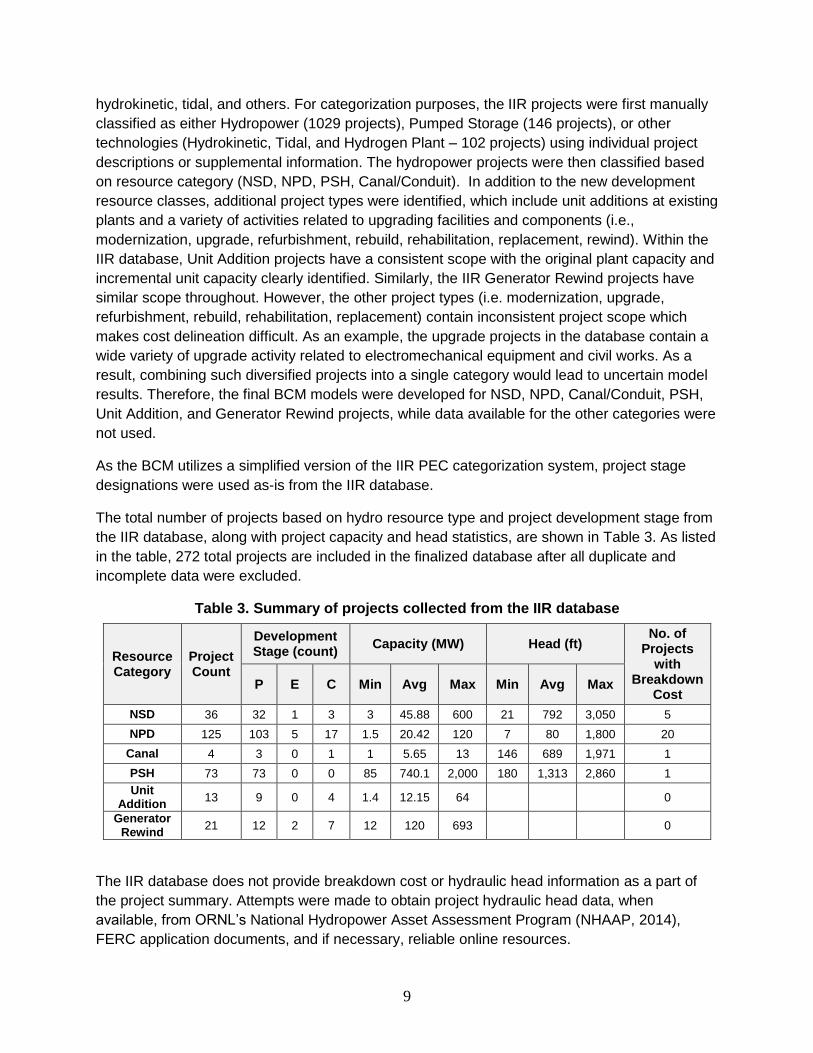
The total number of projects based on hydro resource type and project development stage from
the IIR database, along with project capacity and head statistics, are shown in Table 3. As listed
in the table, 272 total projects are included in the finalized database after all duplicate and
incomplete data were excluded.
Table 3. Summary of projects collected from the IIR database
Resource Category
Project Count
Development Stage (count)
Capacity (MW) Head (ft) No. of
Projects with
Breakdown Cost
P E C Min Avg Max Min Avg Max
NSD 36 32 1 3 3 45.88 600 21 792 3,050 5
NPD 125 103 5 17 1.5 20.42 120 7 80 1,800 20
Canal 4 3 0 1 1 5.65 13 146 689 1,971 1
PSH 73 73 0 0 85 740.1 2,000 180 1,313 2,860 1
Unit Addition
13 9 0 4 1.4 12.15 64 0
Generator Rewind
21 12 2 7 12 120 693 0
The IIR database does not provide breakdown cost or hydraulic head information as a part of
the project summary. Attempts were made to obtain project hydraulic head data, when
available, from ORNL’s National Hydropower Asset Assessment Program (NHAAP, 2014),
FERC application documents, and if necessary, reliable online resources.
10
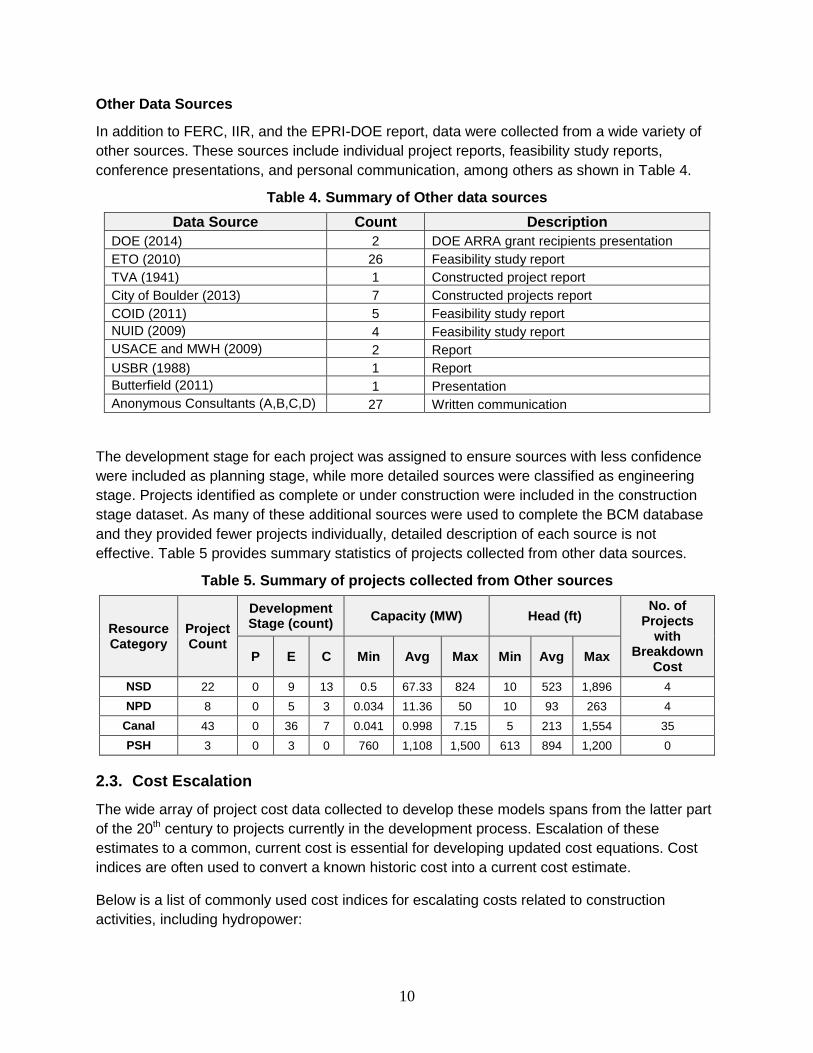
Other Data Sources
In addition to FERC, IIR, and the EPRI-DOE report, data were collected from a wide variety of
other sources. These sources include individual project reports, feasibility study reports,
conference presentations, and personal communication, among others as shown in Table 4.
Table 4. Summary of Other data sources
Data Source Count Description
DOE (2014) 2 DOE ARRA grant recipients presentation
ETO (2010) 26 Feasibility study report
TVA (1941) 1 Constructed project report
City of Boulder (2013) 7 Constructed projects report
COID (2011) 5 Feasibility study report
NUID (2009) 4 Feasibility study report
USACE and MWH (2009) 2 Report
USBR (1988) 1 Report
Butterfield (2011) 1 Presentation
Anonymous Consultants (A,B,C,D) 27 Written communication
The development stage for each project was assigned to ensure sources with less confidence
were included as planning stage, while more detailed sources were classified as engineering
stage. Projects identified as complete or under construction were included in the construction
stage dataset. As many of these additional sources were used to complete the BCM database
and they provided fewer projects individually, detailed description of each source is not
effective. Table 5 provides summary statistics of projects collected from other data sources.
Table 5. Summary of projects collected from Other sources
Resource Category
Project Count
Development Stage (count)
Capacity (MW) Head (ft) No. of
Projects with
Breakdown Cost
P E C Min Avg Max Min Avg Max
NSD 22 0 9 13 0.5 67.33 824 10 523 1,896 4
NPD 8 0 5 3 0.034 11.36 50 10 93 263 4
Canal 43 0 36 7 0.041 0.998 7.15 5 213 1,554 35
PSH 3 0 3 0 760 1,108 1,500 613 894 1,200 0
2.3. Cost Escalation
The wide array of project cost data collected to develop these models spans from the latter part
of the 20th century to projects currently in the development process. Escalation of these
estimates to a common, current cost is essential for developing updated cost equations. Cost
indices are often used to convert a known historic cost into a current cost estimate.
Below is a list of commonly used cost indices for escalating costs related to construction
activities, including hydropower:

11
1. U.S. Bureau of Reclamation (USBR) Construction Cost Trends (CCT) (USBR, 2013)
2. U.S. Army Corps of Engineers (USACE) Civil Works Construction Cost Index System
(CWCCIS) (USACE, 2013a)
3. Engineering News-Record (ENR) Construction Cost Indices (ENR, 2013)
4. RS Means Historical Cost Indices (RSMeans, 2013)
The USBR CCT reflects cost changes for construction activities relevant to the organization,
which primarily include hydroelectric projects. The original indices were derived from the costs
of plants constructed by the USBR. Since the mid-1980’s, the USBR has engaged in fewer
construction projects and no large hydropower projects. Accordingly, the CCT has since been
based on data from the Producer Price Indices (PPI) (BLS, 2014), Price Trends for Federal-Aid
Highway Construction (FHWA, 2014), and ENR, using actual field data to confirm its results
when possible. The CCT consists of 35 construction index categories, a composite index, and
land indices, all compiled quarterly. The construction index categories cover a variety of
essential hydropower infrastructure components, including dams, pumping plants, power plants,
pipelines, canals, tunnels, laterals and drains, switchyards and substations, transmission lines,
roads, bridges, and property.
The USACE CWCCIS includes indices designed specifically for civil works construction. The
CWCCIS provides 19 construction index categories and a composite index and uses several
sources for index development. Quarterly indices have been compiled since 1980, while fiscal
year (FY) values are available since 1968. The construction index categories include several
hydropower-specific features, including reservoirs, dams, power plants, pumping plants,
channels and canals, and floodway control and diversion structures.
ENR Construction Cost Indexes (CCI) is one of the more frequently used (and oldest still in use)
cost indices in the construction industry, (Remer et al., 2008). The CCI uses common labor and
materials prices based on the 20-city average rates and has not changed its calculation basis
since its start in 1908.
RS Means Historical Cost Indexes also allows construction costs to be adjusted between
different years. This index is based on a 30-city average and has been collected since 1963.
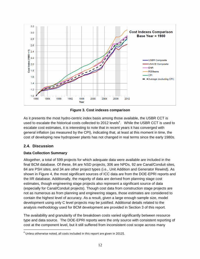
Figure 3 provides a graphical representation of the different cost indexes described, as well as
Consumer Price Index (CPI), from 1980 to 2012. All index values have been adjusted to a 1980
base year for comparison. In the figure, gray areas correspond to historical US economic
recessions and 1980 represents a base year.
12
Figure 3. Cost indexes comparison
As it presents the most hydro-centric index basis among those available, the USBR CCT is
used to escalate the historical costs collected to 2012 levels4. While the USBR CCT is used to
escalate cost estimates, it is interesting to note that in recent years it has converged with
general inflation (as measured by the CPI), indicating that, at least at this moment in time, the
cost of developing new hydropower plants has not changed in real terms since the early 1980s.
2.4. Discussion
Data Collection Summary
Altogether, a total of 599 projects for which adequate data were available are included in the
final BCM database. Of these, 84 are NSD projects, 306 are NPDs, 92 are Canal/Conduit sites,
84 are PSH sites, and 34 are other project types (i.e., Unit Addition and Generator Rewind). As
shown in Figure 4, the most significant sources of ICC data are from the DOE-EPRI reports and
the IIR database. Additionally, the majority of data are derived from planning stage cost
estimates, though engineering stage projects also represent a significant source of data
(especially for Canal/Conduit projects). Though cost data from construction stage projects are
not as numerous as from planning and engineering stages, those estimates are considered to
contain the highest level of accuracy. As a result, given a large enough sample size, model
development using only C level projects may be justified. Additional details related to the
analysis methodology used for BCM development are provided in Section 3 of this report.
The availability and granularity of the breakdown costs varied significantly between resource
type and data source. The DOE-EPRI reports were the only source with consistent reporting of
cost at the component level, but it still suffered from inconsistent cost scope across many
4 Unless otherwise noted, all costs included in this report are given in 2012$.

13
projects, primarily those in the planning stage. Within the other sources, a construction stage
estimate may have been available from IIR, but breakdown costs were only available from
outdated FERC cost estimates. Ultimately, costs were necessarily primarily handled at the level
of total ICC, but issues of unclear scope suggest further data collection could improve the
accuracy of the collected data. However, in Section 4, where breakdown cost data is available it
is presented to add context to the models developed from the total ICC data. Future efforts will
focus on detailed data collection to refine the boundaries of the ICC cost prediction tools.
Figure 4. Finalized BCM data project count by data source, project development stage,
and resource category
The Current Cost of Constructing New Hydropower Resources
Examining the subset of cost data collected from those projects that have either been
constructed or are actively under construction (c-stage) provides insight into the relative
economics of modern hydropower development. Table 6 describes the construction-stage data
for recent hydropower projects in the U.S.5. The lack of recent pumped storage development in
the U.S. resulted in a complete lack of c-stage PSH data, while completed existing generator
rewind and unit addition projects were all taken from the IIR database. Overall, the bulk of the
construction stage data collected for the development of the BCMs was focused on those
resource classes that added power to unpowered sites and reaches (i.e. NSD, NPD, and
Canals).
Table 6 - Summary of projects with actual costs (C-stage)
5 Given limited U.S. data, Canadian projects are included in the development of the NSD ICC models. Due to the
lack of generation data they are not visualized here.
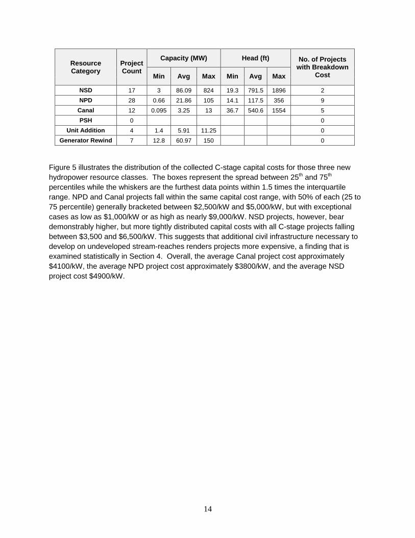
14
Resource Category
Project Count
Capacity (MW) Head (ft) No. of Projects with Breakdown
Cost Min Avg Max Min Avg Max
NSD 17 3 86.09 824 19.3 791.5 1896 2
NPD 28 0.66 21.86 105 14.1 117.5 356 9
Canal 12 0.095 3.25 13 36.7 540.6 1554 5
PSH 0 0
Unit Addition 4 1.4 5.91 11.25 0
Generator Rewind 7 12.8 60.97 150 0
Figure 5 illustrates the distribution of the collected C-stage capital costs for those three new
hydropower resource classes. The boxes represent the spread between 25th and 75th
percentiles while the whiskers are the furthest data points within 1.5 times the interquartile
range. NPD and Canal projects fall within the same capital cost range, with 50% of each (25 to
75 percentile) generally bracketed between $2,500/kW and $5,000/kW, but with exceptional
cases as low as $1,000/kW or as high as nearly $9,000/kW. NSD projects, however, bear
demonstrably higher, but more tightly distributed capital costs with all C-stage projects falling
between $3,500 and $6,500/kW. This suggests that additional civil infrastructure necessary to
develop on undeveloped stream-reaches renders projects more expensive, a finding that is
examined statistically in Section 4. Overall, the average Canal project cost approximately
$4100/kW, the average NPD project cost approximately $3800/kW, and the average NSD
project cost $4900/kW.

15
Figure 5 - Capital costs of recently developed hydropower facilities
Assessing project economics on a lifecycle basis using levelized cost of energy (LCOE) as a
metric tells a different story. In order to estimate LCOE, plant-specific generation estimates for
U.S. projects were collected along alongside capital costs, and operations and maintenance
costs (O&M) is approximated as 2% of ICC per year—Version 2 of this report will include explicit
models for estimating O&M based on design characteristics.
As can be seen in Figure 6, the LCOE of recent developments in all three resources classes is
generally similar. All have median LCOEs of approximately $110/MWh, and generally fall within
more narrow bounds than ICC alone—this convergence is driven by two factors: (1) the fact that
only economically competitive projects will be developed and constructed—therefore high ICC
projects require higher capacity factors for competitive LCOE—and (2) accordingly, that the
NSD projects have higher capacity factors than the canal projects. Projects constructed on
existing water supply infrastructure such as canals are only able to produce power when flows
are scheduled to meet water demands. Oftentimes these projects may see entire seasons
(such as winter) with no water available for electricity generation.
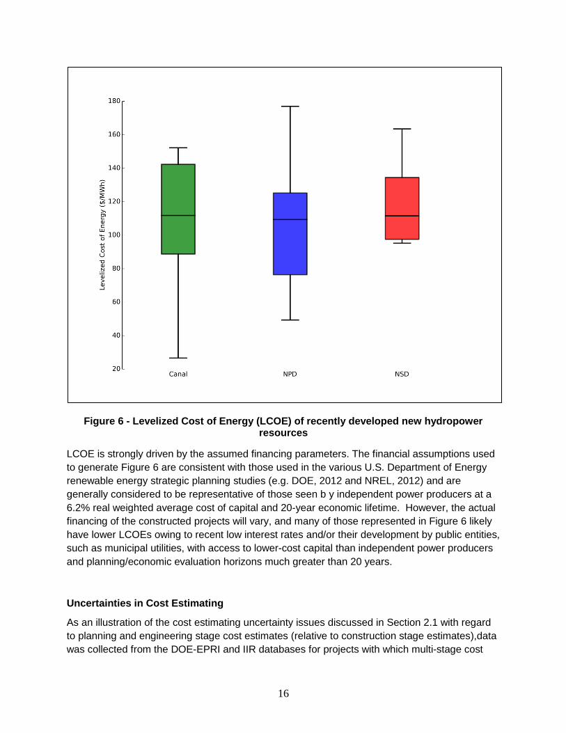
16
Figure 6 - Levelized Cost of Energy (LCOE) of recently developed new hydropower resources
LCOE is strongly driven by the assumed financing parameters. The financial assumptions used
to generate Figure 6 are consistent with those used in the various U.S. Department of Energy
renewable energy strategic planning studies (e.g. DOE, 2012 and NREL, 2012) and are
generally considered to be representative of those seen b y independent power producers at a
6.2% real weighted average cost of capital and 20-year economic lifetime. However, the actual
financing of the constructed projects will vary, and many of those represented in Figure 6 likely
have lower LCOEs owing to recent low interest rates and/or their development by public entities,
such as municipal utilities, with access to lower-cost capital than independent power producers
and planning/economic evaluation horizons much greater than 20 years.
Uncertainties in Cost Estimating
As an illustration of the cost estimating uncertainty issues discussed in Section 2.1 with regard
to planning and engineering stage cost estimates (relative to construction stage estimates),data
was collected from the DOE-EPRI and IIR databases for projects with which multi-stage cost

17
estimates (from planning stage to construction stage) and compared. Table 7 provides
comparative information for 8 DOE-EPRI projects for which planning (P), engineering (E), and
construction (C) data were available (that is, those projects present on all of Volumes 1, 2, and
3).
Table 7. Comparison between planning, engineering, and construction stage cost for
DOE-EPRI dataset projects
Project Name Project
Category Construction
Year Capacity
(MW)
ICC ($/kW in 2012$)
P E C
Garland Canal Canal/Conduit 1984 2.7 3,294 4,549 3,216
Garvins Falls NPD 1982 6.5 2,554 2,896 2,796
Great Falls NPD 1983 10.95 2,801 2,477 2,867
Idaho Falls New 1983 24 5,359 4,797 6,394
Jackson Bluff NPD 1984 10.9 3,356 3,108 2,752
Shawmut NPD 1982 4.112 4,097 1,644 3,124
Turlock NPD 1981 3.26 3,668 3,307 3,590
Upper Mechanicsville NPD 1984 16.8 5,333 5,531 6,383
Average 9.9 3,808 3,539 3,890
Similarly,
Table 8 demonstrates the differences in project cost across different project development stages for 13 IIR projects with historical estimates spanning all three stages of development
Table 8. Comparison between actual project cost, engineering stage, and feasibility stage
cost for IIR dataset
Project Name Project
Category Construction
Year Capacity
(MW)
ICC ($/kW in 2012$)
P E C
1 NPD 2014 4.6 5,784 5,239 3,760
2 NPD 2014 5.6 2,493 3,571 3,321
3 NPD 2014 6 1,861 2,411 2,325
4 NPD 2014 7 6,651 5,429 5,048
5 NPD 2008 12 1,919 1,745 1,380
6 Canal/Conduit 2011 13 1,850 2,502 2,387
7 NPD 2014 16 5,748 2,104 2,092
8 NPD 2013 30 1,110 1,724 2,250
9 NPD 2012 31.5 1,684 2,678 2,413
10 NPD 2014 35 2,660 8,868 7,971
11 NPD 2013 75 2,455 6,506 5,786
12 NPD 2014 84 1,754 5,370 4,605
13 NPD 2014 105 3,699 3,614 4,464
Average 32.7 3,051 3,982 3,677

18
Comparison of estimate cost trajectories reveals two major characteristics: 1) final construction
costs are not uniformly higher or lower than earlier stage estimates and 2) relative stage cost
varies between the data sources. The second characteristic noted derives from the observation
that DOE-EPRI projects generally contain more variation in how cost changes from P to E to C
stage. This can likely be partially attributed to differences in data collection practices, however,
in the case of the DOE-EPRI data set, the unique volatile inflation environment in late1970s and
early 1980s may have contributed to decreased accuracy for cost estimates at planning or
engineering stages of development. The more recent IIR dataset shows that engineering stage
data is generally more accurate than those derived from planning stage estimates, as would be
expected.
3. Analysis Methodology
3.1. Model Development
Historically, hydropower costs have been well-represented by power-law relationships between
ICC and key plant parameters, such as installed capacity (INL, 2003) or to capture the cost
dynamics of high and low-head hydropower plants, both capacity and design head (Gordon,
1979). Except where otherwise discussed, the development of the cost models in this
document relies on the capacity-head relationship (shown below) to better cost the relatively
low-head resources remaining in the U.S.
𝐼𝐶𝐶 = 𝑎𝑃𝑏𝐻𝑐
where
𝐼𝐶𝐶 = Initial Capital Cost,
𝑃 = Capacity (in MW),
𝐻 = Hydraulic Head (in ft),
𝑎 = Slope coefficient,
𝑏 = Capacity exponent, and
𝑐 = Head exponent.
Methodologically, power-law relationships can be fit using a variety of methods. Traditionally,
this has been done using log-transformed variables in a linear regression or directly via non-
linear least squares regression. The appropriate choice of method is contingent on the
distribution of error in order to avoid violating the assumptions of least squares regression
methods (Xiao et al, 2011) - geometric (multiplicative) errors become normal on a log-scale,
while additive (arithmetic) errors are only appropriately modeled when untransformed.
Conceptually, error for ICC data should be multiplicative (i.e. $10,000,000 project should expect
cost deviations from prediction to be 10x a $1,000,000 project); this is also consistent with the
AACE practice of using percentage based estimating ranges. Therefore, log transformed linear
regression is used to fit the ICC power law models.

19
The use of linear regression requires a linear relationship between the dependent and
independent variables, and so, the power relationship is converted to a linear relationship by
taking log values of the variables (ICC, P, and H) on both the left and right sides the equation :
log(𝐼𝐶𝐶) = 𝑙𝑜𝑔(𝑎) + 𝑏 log(𝑃) + 𝑐 log(𝐻) + 𝜀
The mean of error term (𝜀) of log transformed data will be zero, but this assumption does not
necessarily hold upon retransformation of the data into the original untransformed scale
(Newman, 1993), biasing any estimates derived from the directly retransformed model.
Therefore, the error term needs to be explicitly incorporated by adjusting the power relationship:
𝐼𝐶𝐶 = 𝑎𝑃𝑏𝐻𝑐𝑒𝜀
For this study, the Smearing Estimator (Duan, 1983), a non-parametric method, is used to
calculate the bias correction, 𝑒𝜀:.
𝑒𝜀 = ∑ exp(𝑒𝑖)𝑖=𝑁
𝑖=1
𝑁
where, 𝑒𝑖 = Residuals from regression model, 𝑁 = Sample size. The error term 𝑒𝜀 is
called smear correction and is also referred to as bias correction.
3.2. Model Selection and Evaluation
Model Confidence Scoring
In the development of the BCMs, a variety of different data subsets were evaluated both to
understand the sources of cost variation and to ultimately select the models that best represent
the cost of developing the remaining U.S. hydropower resources. To consistently evaluate the
alternative model options within each resource class, a quantitative evaluation system was
developed to rank models based on the following series of metrics related to (1) attributes of the
data used in the development of the model, and (2) the overall quality of the model itself:
Data
o Data Quality (project development stage)
o Data Scope and Consistency
o Data Vintage (age of cost estimate)
Model Quality
o Sample Size
o Data QA/QC
o Goodness of Fit
o Validation
o Application Range

20
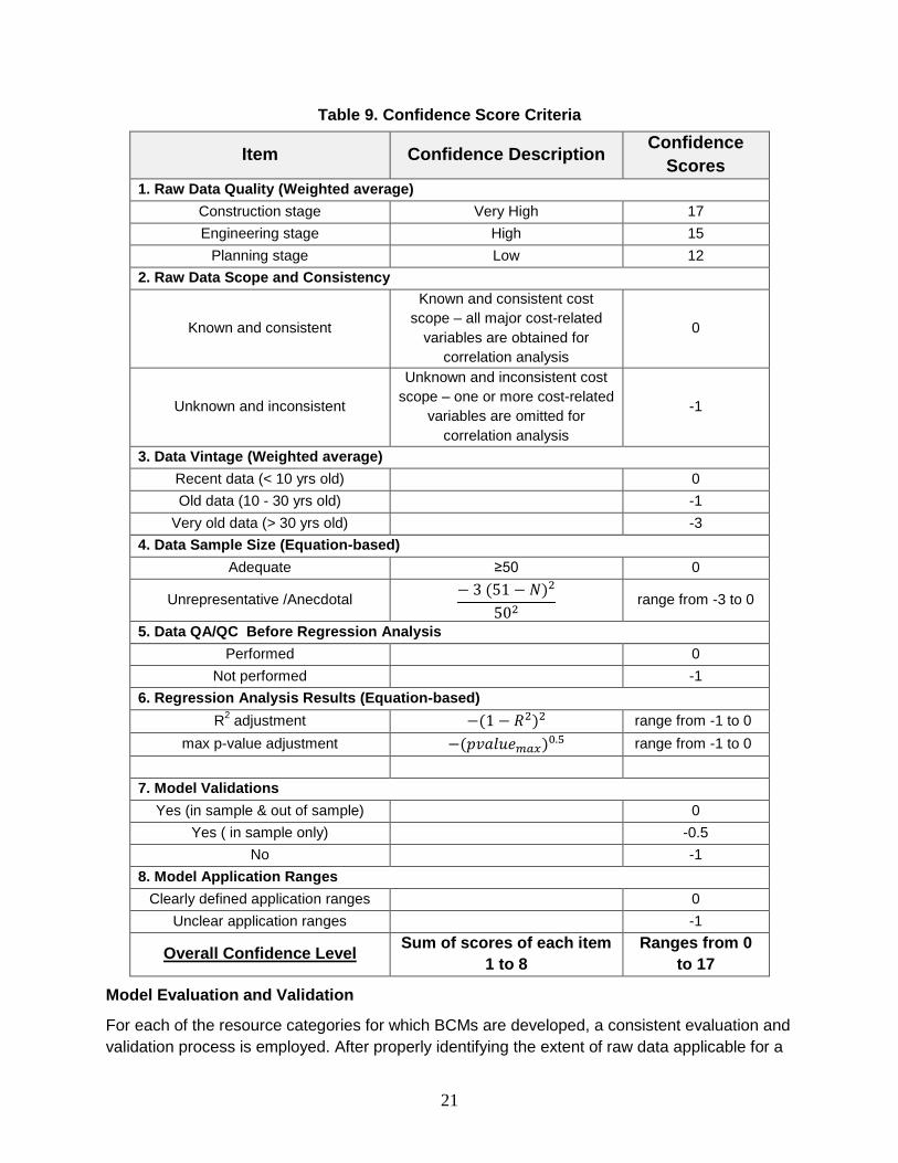
Table 9 shows how the metrics used for evaluating model confidence are quantified. The
confidence level associated with each data source are quantified using Items 1 through 3, while
the overall model results, reliability, and application are scored using Items 4 through 8.
Individual model scores for Items 1 and 3 are weighted according to the number of projects
included from each development stage and vintage category, respectively. A model confidence
score in this report is sum of score of each item 1 to 8. Overall, the range of potential confidence
scores range from 0 to 17.
21
Table 9. Confidence Score Criteria
Item Confidence Description Confidence
Scores
1. Raw Data Quality (Weighted average)
Construction stage Very High 17
Engineering stage High 15
Planning stage Low 12
2. Raw Data Scope and Consistency
Known and consistent
Known and consistent cost
scope – all major cost-related
variables are obtained for
correlation analysis
0
Unknown and inconsistent
Unknown and inconsistent cost
scope – one or more cost-related
variables are omitted for
correlation analysis
-1
3. Data Vintage (Weighted average)
Recent data (< 10 yrs old)
0
Old data (10 - 30 yrs old)
-1
Very old data (> 30 yrs old)
-3
4. Data Sample Size (Equation-based)
Adequate ≥50 0
Unrepresentative /Anecdotal − 3 (51 − 𝑁)2
502 range from -3 to 0
5. Data QA/QC Before Regression Analysis
Performed
0
Not performed
-1
6. Regression Analysis Results (Equation-based)
R2 adjustment −(1 − 𝑅2)2 range from -1 to 0
max p-value adjustment −(𝑝𝑣𝑎𝑙𝑢𝑒𝑚𝑎𝑥)0.5 range from -1 to 0
7. Model Validations
Yes (in sample & out of sample)
0
Yes ( in sample only)
-0.5
No
-1
8. Model Application Ranges
Clearly defined application ranges
0
Unclear application ranges
-1
Overall Confidence Level Sum of scores of each item
1 to 8
Ranges from 0
to 17
Model Evaluation and Validation
For each of the resource categories for which BCMs are developed, a consistent evaluation and
validation process is employed. After properly identifying the extent of raw data applicable for a
22
particular category, projects which are identified as duplicates or outliers are removed, while
additional data limitations (e.g., lack of head data) may limit the final database size. The
finalized database is then evaluated across various development stages to identify the major
independent variables to include in the models based on graphical representations and
regression analysis. The resulting cost model equations are assessed for validity, while the
coefficient of determination (R2) and p-values are compared to assess overall model
performance and suitability. In the end, a recommended model is identified based on confidence
score results, though alternative models are presented in Appendix A.
In addition to presenting the recommended model, the recommended NPD and NSD models
are also compared against other available cost models: INL models (INL, 2003), USACE model
(USACE, 2013b), both from this BCM effort and from literature. In-sample validation is also
performed (see Appendix A). Finally, average categorical breakdown costs are presented for
the models, with breakdowns for alternative models provided in Appendix A.
4. Model Results
Section 4 describes the evaluation and validation for the NPD, NSD, Canal/Conduit, PSH, Unit
Addition, and Generator Rewind baseline cost models and presents average project breakdown
costs. The application ranges of a cost model should be clearly defined and validated based on
the scope of raw cost data that are used to derive the model. When using any cost model,
whether found in literature or in this report, caution should be exercised if extrapolating the cost
curve beyond its intended application ranges (e.g., some cost equations were developed for
large hydro only and will bring “bias” for small hydro cost estimating). In an attempt to
adequately identify application ranges for the recommended models, information is provided for
each resource category in Section 4.
4.1. Non-powered Dams (NPDs)
Starting with a total of 436 NPD projects, 119 were identified as duplicates, with another 10
excluded due to a lack of hydraulic head information. In addition, 1 project containing a per-kW
cost above $78,000 was identified as an outlier and subsequently removed. The final NPD
database comprises information from a total of 306 projects, which were disaggregated into
various categories based on project development stage, project capacity, and hydraulic head.
The results herein represent the finalized dataset containing 306 NPD projects.
Data Statistics
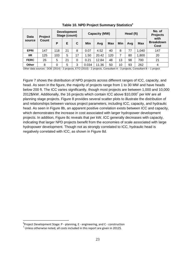
Table 10 provides summary statistics for the NPD projects by data source. The majority of data
were taken from EPRI or IIR, and the project capacities range from 34 kW to 120 MW. Over
70% of the data contain planning stage development costs. In addition, breakdown costs were
collected for a total of 192 NPD projects.
23
Table 10. NPD Project Summary Statistics6
Data source
Project Count
Development Stage (count)
Capacity (MW) Head (ft) No. of
Projects with
Breakdown Cost
P E C Min Avg Max Min Avg Max
EPRI 147 118 21 8 0.07 4.52 40 8 77 1,040 147
IIR 125 103 5 17 1.50 20.42 120 7 80 1,800 20
FERC 26 5 21 0 0.21 12.84 48 13 98 700 21
Other 8 0 5 3 0.034 11.36 50 10 93 262 4 Other data sources : DOE (2014) - 2 projects, ETO (2010) - 2 projects, Consultant A - 3 projects, Consultant B – 1 project
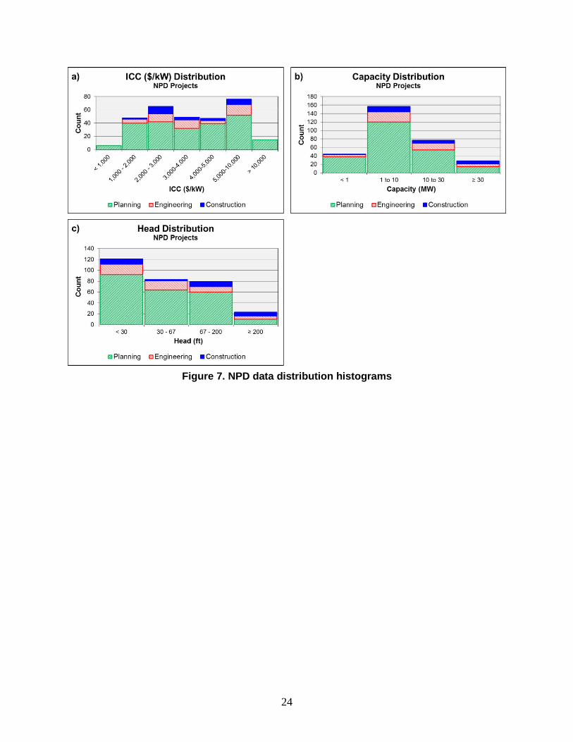
Figure 7 shows the distribution of NPD projects across different ranges of ICC, capacity, and
head. As seen in the figure, the majority of projects range from 1 to 30 MW and have heads
below 200 ft. The ICC varies significantly, though most projects are between 1,000 and 10,000
2012$/kW. Additionally, the 16 projects which contain ICC above $10,0007 per kW are all
planning stage projects. Figure 8 provides several scatter plots to illustrate the distribution of
and relationships between various project parameters, including ICC, capacity, and hydraulic
head. As seen in Figure 8b, an apparent positive correlation exists between ICC and capacity,
which demonstrates the increase in cost associated with larger hydropower development
projects. In addition, Figure 8c reveals that per kW, ICC generally decreases with capacity,
indicating that larger NPD projects benefit from the economies of scale associated with large
hydropower development. Though not as strongly correlated to ICC, hydraulic head is
negatively correlated with ICC, as shown in Figure 8d.
6Project Development Stage: P - planning, E - engineering, and C - construction
7 Unless otherwise noted, all costs included in this report are given in 2012$.
24
Figure 7. NPD data distribution histograms
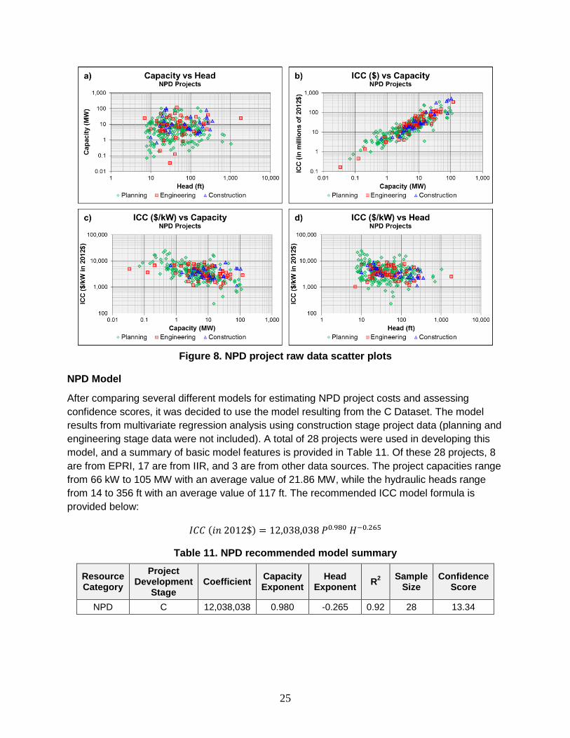
25
Figure 8. NPD project raw data scatter plots
NPD Model
After comparing several different models for estimating NPD project costs and assessing
confidence scores, it was decided to use the model resulting from the C Dataset. The model
results from multivariate regression analysis using construction stage project data (planning and
engineering stage data were not included). A total of 28 projects were used in developing this
model, and a summary of basic model features is provided in Table 11. Of these 28 projects, 8
are from EPRI, 17 are from IIR, and 3 are from other data sources. The project capacities range
from 66 kW to 105 MW with an average value of 21.86 MW, while the hydraulic heads range
from 14 to 356 ft with an average value of 117 ft. The recommended ICC model formula is
provided below:
𝐼𝐶𝐶 (𝑖𝑛 2012$) = 12,038,038 𝑃0.980 𝐻−0.265
Table 11. NPD recommended model summary
Resource Category
Project Development
Stage Coefficient
Capacity Exponent
Head Exponent
R2
Sample Size
Confidence Score
NPD C 12,038,038 0.980 -0.265 0.92 28 13.34

26
Overall, the C model provides the highest confidence score of 13.34, which exceeds the EC and
PEC model scores of 12.35 and 9.18, respectively, identifying the C model as the ORNL
recommended model for NPDs.
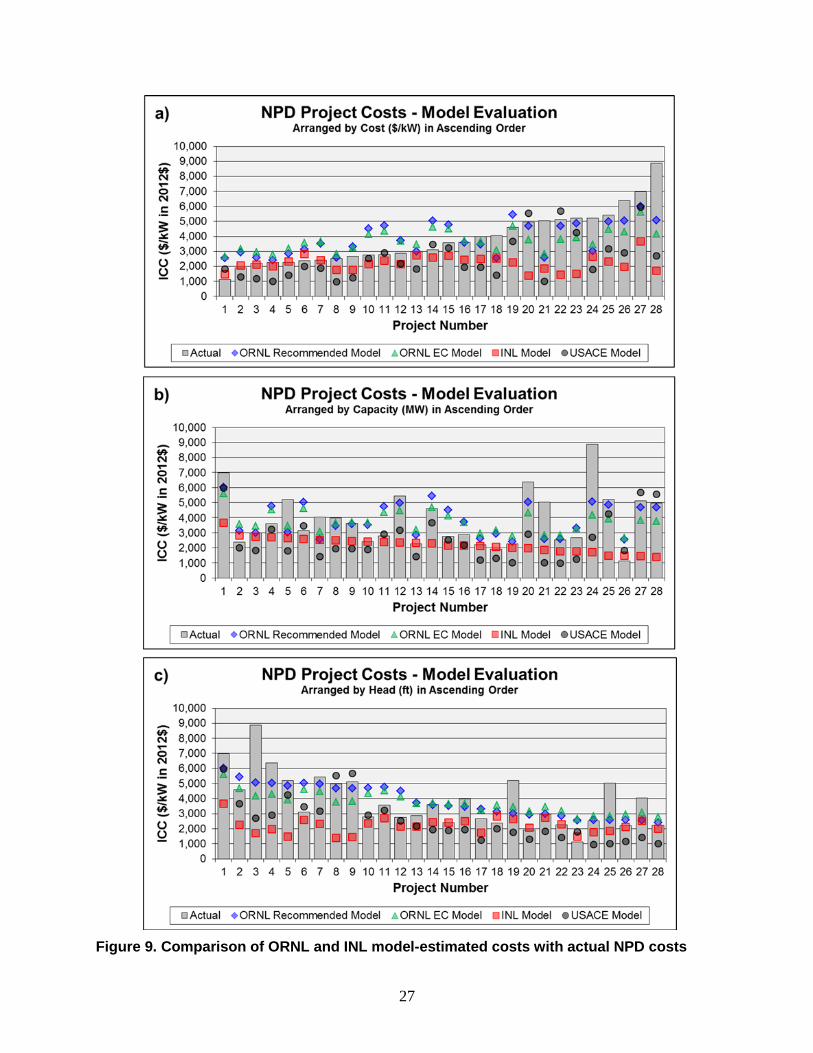
To further validate the model, graphical in-sample validation was performed with no noticeable
bias identified. Figure 9 provides a comparison between the recommended NPD model
developed for this report, the alternative NPD model developed from the EC dataset included
given the closeness in confidence score, the INL model (INL, 2003) developed for construction
of dams without power, the USACE resource assessment model (USACE, 2013b)8, and the
actual project costs included in the C Dataset. As seen in Figure 9, for most projects the ORNL
recommended model estimates higher ICC compared to the other models. Compared with
actual cost, the ORNL recommended model tends to better approximate project costs than the
other models. In addition, the C model generally overestimates ICC for the lower per kW cost
projects and underestimates ICC for the higher per kW cost projects (Figure 9a). As seen in
Figure 9b and Figure 9c, the recommended model’s relative error is largely independent of
variation in capacity and head. Compared with the EC model, the recommended model provides
very similar ICC estimates, though a more noticeable difference is seen for the lower head
projects (Figure 9c). As expected, the INL model shows significant bias in estimating ICC for low
head projects, as the model provides only a univariate estimate based on capacity (Figure 9c).
The average actual project ICC for the 28 constructed projects is $3,833, while the
recommended ORNL, INL, and USACE models produce average per kW costs of $3,844,
$2,199, and $2,530, respectively. As the recommended ORNL model was developed based on
regression analysis using the same set of 28 constructed projects, the model necessarily
produces the best approximation for the actual cost, and further data collection will allow for the
model to be benchmarked against out of sample data points, and more robustly identify cost
drivers at the component level.
8 It is important to note that the USACE model explicitly attempts to size plants and select turbine number and
type based on site head and capacity parameters. In its application here to the C data set, static values of head and capacity are used. As discussed in the executive summary and introduction, this and other more sophisticated modeling approaches should yield estimates with increased accuracy if detailed site-specific data such as flow and head duration curves were available.
27
Figure 9. Comparison of ORNL and INL model-estimated costs with actual NPD costs

28
Although the C model is recommended for NPD costing application, numerous other models
were developed and compared during the model development and validation stages. Details on
the additional NPD models evaluated and more specific discussion are provided in Appendix A.
Breakdown Costs
Although the recommended ICC model for NPDs uses just C stage projects, breakdown cost
data were only available for 2 construction stage NPD projects; consequently, both E and C
stage projects are used for illustration. Figure 10 provides average breakdown cost statistics for
36 engineering and 2 construction stage NPD projects. As seen in the chart, the civil works and
equipment costs constitute about 81% of the total NPD project development cost, with
equipment costs representing the primary cost driver. Additional breakdown cost distributions
based on hydraulic head and capacity ranges were developed and are provided in Appendix A.
Figure 10. Breakdown cost distribution for NPD projects (EC dataset)
4.2. New Stream-reach Development (NSDs)
Starting with a total of 95 NSD projects, 7 were identified as duplicates, with another 3 excluded
due to a lack of hydraulic head information. In addition, 1 project containing a per-kW cost
above $96,000 was identified as an outlier and subsequently removed. The final NSD database
comprises information from a total of 84 projects, which were disaggregated into various
categories based on project development stage, project capacity, and hydraulic head. The
results herein represent the finalized dataset containing the 84 NSD projects.
29
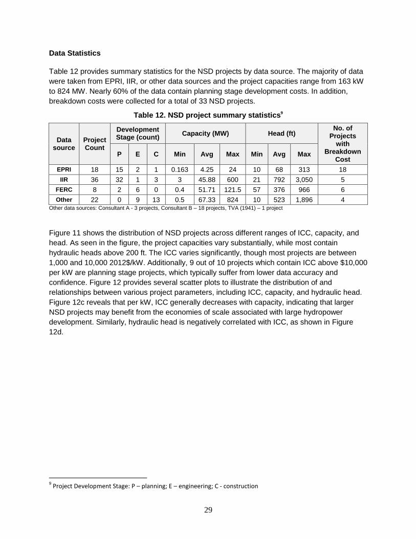
Data Statistics
Table 12 provides summary statistics for the NSD projects by data source. The majority of data
were taken from EPRI, IIR, or other data sources and the project capacities range from 163 kW
to 824 MW. Nearly 60% of the data contain planning stage development costs. In addition,
breakdown costs were collected for a total of 33 NSD projects.
Table 12. NSD project summary statistics9
Data source
Project Count
Development Stage (count)
Capacity (MW) Head (ft) No. of
Projects with
Breakdown Cost
P E C Min Avg Max Min Avg Max
EPRI 18 15 2 1 0.163 4.25 24 10 68 313 18
IIR 36 32 1 3 3 45.88 600 21 792 3,050 5
FERC 8 2 6 0 0.4 51.71 121.5 57 376 966 6
Other 22 0 9 13 0.5 67.33 824 10 523 1,896 4 Other data sources: Consultant A - 3 projects, Consultant B – 18 projects, TVA (1941) – 1 project
Figure 11 shows the distribution of NSD projects across different ranges of ICC, capacity, and
head. As seen in the figure, the project capacities vary substantially, while most contain
hydraulic heads above 200 ft. The ICC varies significantly, though most projects are between
1,000 and 10,000 2012$/kW. Additionally, 9 out of 10 projects which contain ICC above $10,000
per kW are planning stage projects, which typically suffer from lower data accuracy and
confidence. Figure 12 provides several scatter plots to illustrate the distribution of and
relationships between various project parameters, including ICC, capacity, and hydraulic head.
Figure 12c reveals that per kW, ICC generally decreases with capacity, indicating that larger
NSD projects may benefit from the economies of scale associated with large hydropower
development. Similarly, hydraulic head is negatively correlated with ICC, as shown in Figure
12d.
9 Project Development Stage: P – planning; E – engineering; C - construction

30
Figure 11. NSD project raw data distribution histograms
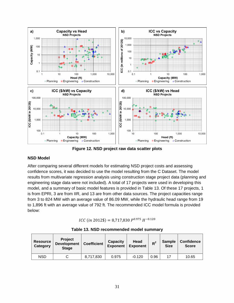
31
Figure 12. NSD project raw data scatter plots
NSD Model
After comparing several different models for estimating NSD project costs and assessing
confidence scores, it was decided to use the model resulting from the C Dataset. The model
results from multivariate regression analysis using construction stage project data (planning and
engineering stage data were not included). A total of 17 projects were used in developing this
model, and a summary of basic model features is provided in Table 13. Of these 17 projects, 1
is from EPRI, 3 are from IIR, and 13 are from other data sources. The project capacities range
from 3 to 824 MW with an average value of 86.09 MW, while the hydraulic head range from 19
to 1,896 ft with an average value of 792 ft. The recommended ICC model formula is provided
below:
𝐼𝐶𝐶 (𝑖𝑛 2012$) = 8,717,830 𝑃0.975 𝐻−0.120
Table 13. NSD recommended model summary
Resource Category
Project Development
Stage Coefficient
Capacity Exponent
Head Exponent
R2
Sample Size
Confidence Score
NSD C 8,717,830 0.975 -0.120 0.96 17 10.65

32
Overall, the C model provides the highest confidence score of 12.65, which exceeds the EC and
PEC model scores of 11.97 and 10.19, respectively; this identifies the C model as the ORNL
recommended model for NSDs.
To further validate the model, graphical in-sample validation was performed, with no noticeable
bias identified. Figure 13 provides a comparison between the recommended NSD model
developed for this report, the alternative NSD model developed from the EC dataset, the INL
model (INL, 2003) developed for construction of undeveloped sites, and the actual project costs
included in the C Dataset. As seen in Figure 13, for most projects with actual cost data
available, the ORNL recommended model generally estimates similar or slightly higher ICC
compared to the other models. Compared with actual cost, the ORNL recommended model
tends to better approximate project costs than the INL model. In addition, the C model generally
overestimates ICC for the lower per kW cost projects and underestimates ICC for the higher per
kW cost projects (Figure 13a). As seen in Figure 13b, the recommended model’s relative error
is largely independent of variation in capacity, though the model displays more bias (both
positive and negative) for the lower head projects (Figure 13c). Compared with the EC model,
the recommended model provides very similar ICC estimates, though a more noticeable
difference is seen for the higher head projects (Figure 13c). As expected, the INL model shows
significant bias in estimating ICC for low head projects, as the model provides only simplified
univariate estimation based on capacity (Figure 13c). The average actual project ICC for the 17
constructed projects is $3,885, while the recommended ORNL and INL models produce
average per kW costs of $3,882 and $3,631, respectively. As the recommended ORNL model
was developed based on regression analysis using the same set of 17 constructed projects, the
model necessarily produces the best approximation for the actual cost, and in the future, out-of-
sample validation should be performed to further evaluate model accuracy.
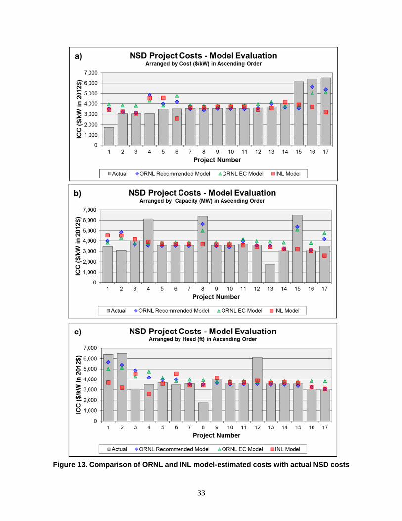
33
Figure 13. Comparison of ORNL and INL model-estimated costs with actual NSD costs
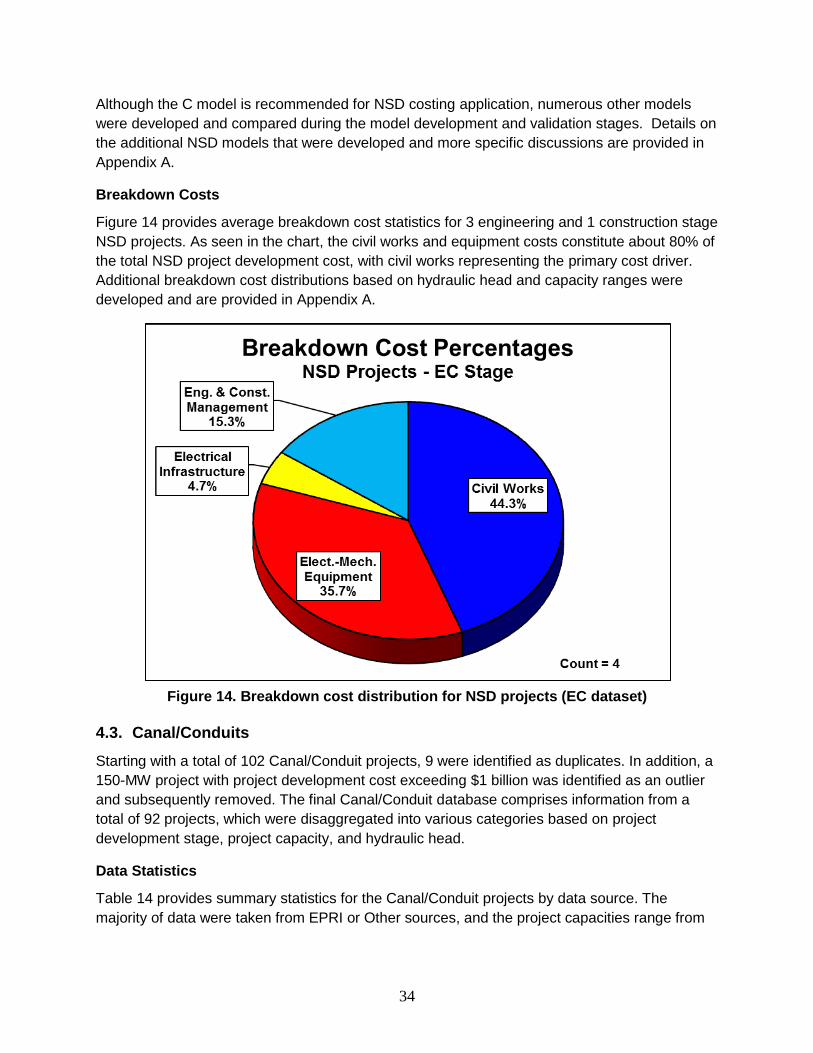
34
Although the C model is recommended for NSD costing application, numerous other models
were developed and compared during the model development and validation stages. Details on
the additional NSD models that were developed and more specific discussions are provided in
Appendix A.
Breakdown Costs
Figure 14 provides average breakdown cost statistics for 3 engineering and 1 construction stage
NSD projects. As seen in the chart, the civil works and equipment costs constitute about 80% of
the total NSD project development cost, with civil works representing the primary cost driver.
Additional breakdown cost distributions based on hydraulic head and capacity ranges were
developed and are provided in Appendix A.
Figure 14. Breakdown cost distribution for NSD projects (EC dataset)
4.3. Canal/Conduits
Starting with a total of 102 Canal/Conduit projects, 9 were identified as duplicates. In addition, a
150-MW project with project development cost exceeding $1 billion was identified as an outlier
and subsequently removed. The final Canal/Conduit database comprises information from a
total of 92 projects, which were disaggregated into various categories based on project
development stage, project capacity, and hydraulic head.
Data Statistics
Table 14 provides summary statistics for the Canal/Conduit projects by data source. The
majority of data were taken from EPRI or Other sources, and the project capacities range from

35
41 kW to 15 MW. About 41% of the data contain planning stage development costs. In addition,
breakdown costs were collected for a total of 77 Canal/Conduit projects.
Table 14. Canal/Conduit project summary statistics10
Data source
Project Count
Development Stage (count)
Capacity (MW) Head (ft) No. of
Projects with
Breakdown Cost
P E C Min Avg Max Min Avg Max
EPRI 36 31 1 4 0.1 2.378 15 21 176.6 904 36
IIR 4 3 0 1 1 5.645 13 146 689.3 1,971 1
FERC 9 4 5 0 0.225 1.72 6.15 34 211.2 445 5
Other 43 0 36 7 0.041 0.998 7.15 5 212.7 1,554 35 Other data sources: City of Boulder (2013) – 7 projects, COID (2011) – 5 projects, ETO (2010): 24 projects, NUID (2009) – 4 projects, Butterfield (2011) – 1 project, Consultant C - 1 project, Consultant D – 1 project.
Figure 15 shows the distribution of Canal/Conduit projects across different ranges of ICC,
capacity, and head. Most projects are below 10 MW, but head varies significantly; the
constructed projects generally design heads greater than 200 ft. The ICC varies significantly,
though many project costs are between $5,000 and $10,000 per kW (constructed projects have
generally lower ICC). 10 of the projects which contain ICC above $10,000 per kW are
engineering stage, while the other 3 are planning stage projects. Figure 16 provides several
scatter plots with the distribution of various project parameters, including ICC, capacity, and
hydraulic head. Figure 16c reveals that per kW, ICC generally decreases with capacity,
indicating that larger Canal/Conduit projects benefit from the economies of scale associated
with large hydropower development. Similarly, hydraulic head is negatively correlated with ICC,
as shown in Figure 16d.
10
Project Development Stage: P – planning; E – engineering; C - construction
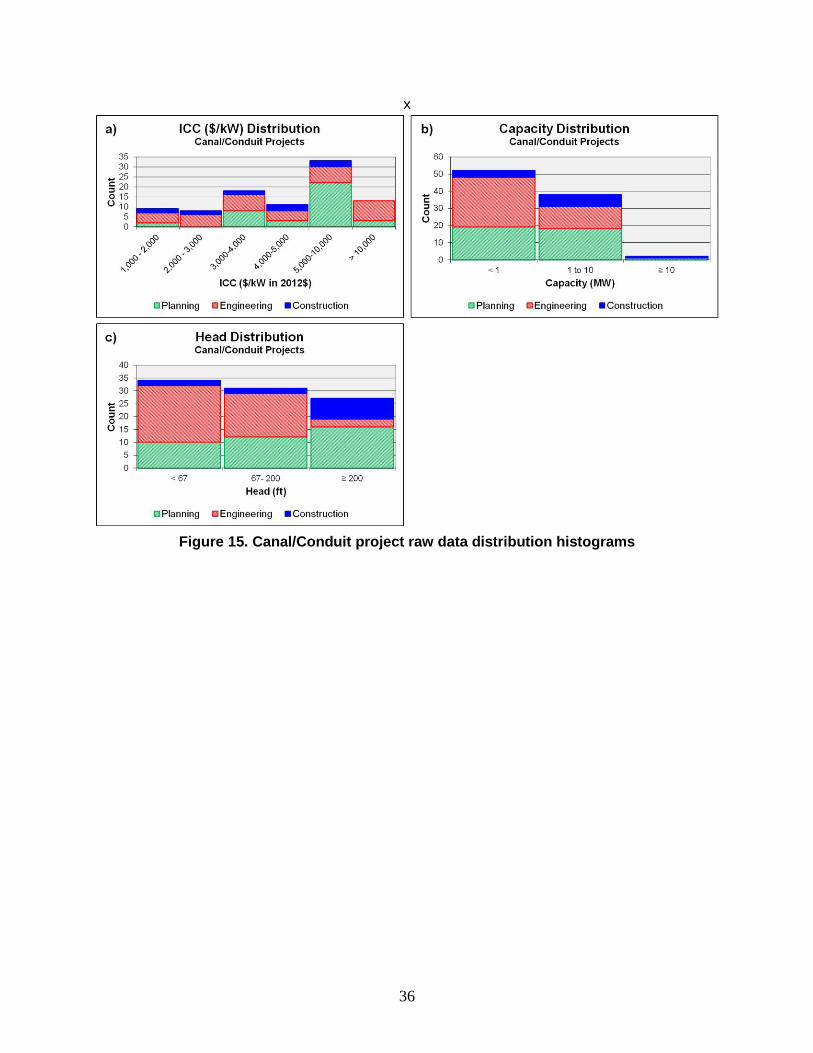
36
x
Figure 15. Canal/Conduit project raw data distribution histograms
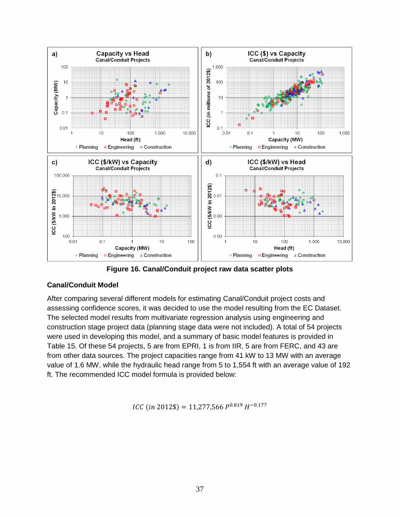
37
Figure 16. Canal/Conduit project raw data scatter plots
Canal/Conduit Model
After comparing several different models for estimating Canal/Conduit project costs and
assessing confidence scores, it was decided to use the model resulting from the EC Dataset.
The selected model results from multivariate regression analysis using engineering and
construction stage project data (planning stage data were not included). A total of 54 projects
were used in developing this model, and a summary of basic model features is provided in
Table 15. Of these 54 projects, 5 are from EPRI, 1 is from IIR, 5 are from FERC, and 43 are
from other data sources. The project capacities range from 41 kW to 13 MW with an average
value of 1.6 MW, while the hydraulic head range from 5 to 1,554 ft with an average value of 192
ft. The recommended ICC model formula is provided below:
𝐼𝐶𝐶 (𝑖𝑛 2012$) = 11,277,566 𝑃0.819 𝐻−0.177
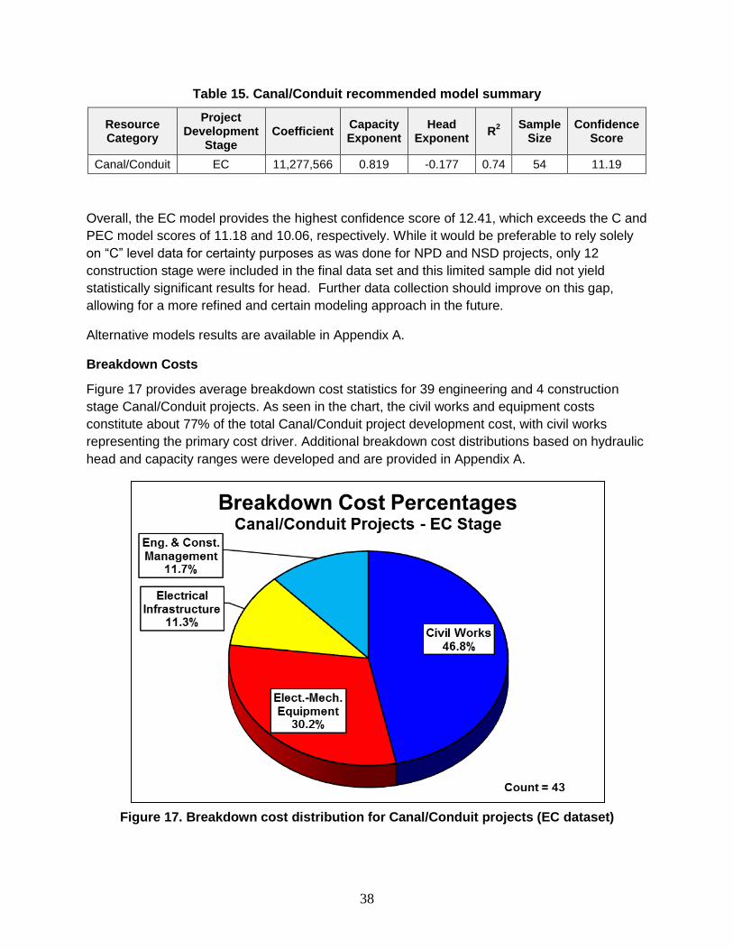
38
Table 15. Canal/Conduit recommended model summary
Resource Category
Project Development
Stage Coefficient
Capacity Exponent
Head Exponent
R2
Sample Size
Confidence Score
Canal/Conduit EC 11,277,566 0.819 -0.177 0.74 54 11.19
Overall, the EC model provides the highest confidence score of 12.41, which exceeds the C and
PEC model scores of 11.18 and 10.06, respectively. While it would be preferable to rely solely
on “C” level data for certainty purposes as was done for NPD and NSD projects, only 12
construction stage were included in the final data set and this limited sample did not yield
statistically significant results for head. Further data collection should improve on this gap,
allowing for a more refined and certain modeling approach in the future.
Alternative models results are available in Appendix A.
Breakdown Costs
Figure 17 provides average breakdown cost statistics for 39 engineering and 4 construction
stage Canal/Conduit projects. As seen in the chart, the civil works and equipment costs
constitute about 77% of the total Canal/Conduit project development cost, with civil works
representing the primary cost driver. Additional breakdown cost distributions based on hydraulic
head and capacity ranges were developed and are provided in Appendix A.
Figure 17. Breakdown cost distribution for Canal/Conduit projects (EC dataset)

39
4.4. Pumped Storage Hydropower (PSH)
Starting with a total of 135 PSH projects, 30 were identified as duplicates, with another 6
excluded due to a lack of capital cost or hydraulic head information. One project with a cost
above $11,000 per kW was removed as an outlier, as was a 760kW planning stage project from
the DOE-EPRI report. This latter project is over 100 times smaller than the next smallest project
(85 MW) and heavily biased model results prior to removal. Additionally, all 14 construction
stage data points were removed—these projects were U.S. historical build, and even when
escalated using the USBR CCT index, were substantially less expensive on a per kW basis than
the remainder of the dataset. This result is consistent with the observation in EPRI (2011) that
PSH costs have appeared to increase at a rate faster than would be expected from general
hydropower cost indices.
The final PSH database comprises information from a total of 83 projects. The data were
disaggregated into various categories based on project development stage, project capacity,
and hydraulic head.
Data Statistics
Table 16 provides summary statistics for the PSH projects by data source. The majority of data
were taken from IIR or FERC data sources, and the project capacities range from 85 MW to
2,000 MW. Roughly 88% of the data contain planning stage development costs. In addition,
breakdown costs were collected for a total of 4 PSH projects.
Table 16. PSH project summary statistics11
Data source
Project Count
Development Stage (count)
Capacity (MW) Head (ft) No. of
Projects with
Breakdown Cost
P E C Min Avg Max Min Avg Max
IIR 73 73 0 0 85 740.1 2,000 180 1,313 2,860 1
FERC 7 0 7 0 280 868.6 1,300 720 1,324 1,866 3
Other 3 0 3 0 760 1,108 1,500 613 894 1,200 0 Other data sources: USACE and MWH (2009) – 2 projects, USBR (1988) – 1 project.
Figure 18 shows the distribution of PSH projects across different ranges of ICC, capacity, and
head. As seen in the figure, the project capacities and heads vary substantially, while most
project ICCs range between $1,000 and $2,000 per kW. All of the projects which with an ICC
below $1,000 per kW are planning stage projects. Figure 19 provides several scatter plots to
illustrate the distribution of and relationships between various project parameters, including ICC,
capacity, and hydraulic head. Figure 19c suggests that per kW, ICC does not decrease
noticeably as the project capacity increases, and the hydraulic head is not strongly correlated
with ICC (Figure 19d).
11
Project Development Stage: P – planning; E – engineering; C - construction
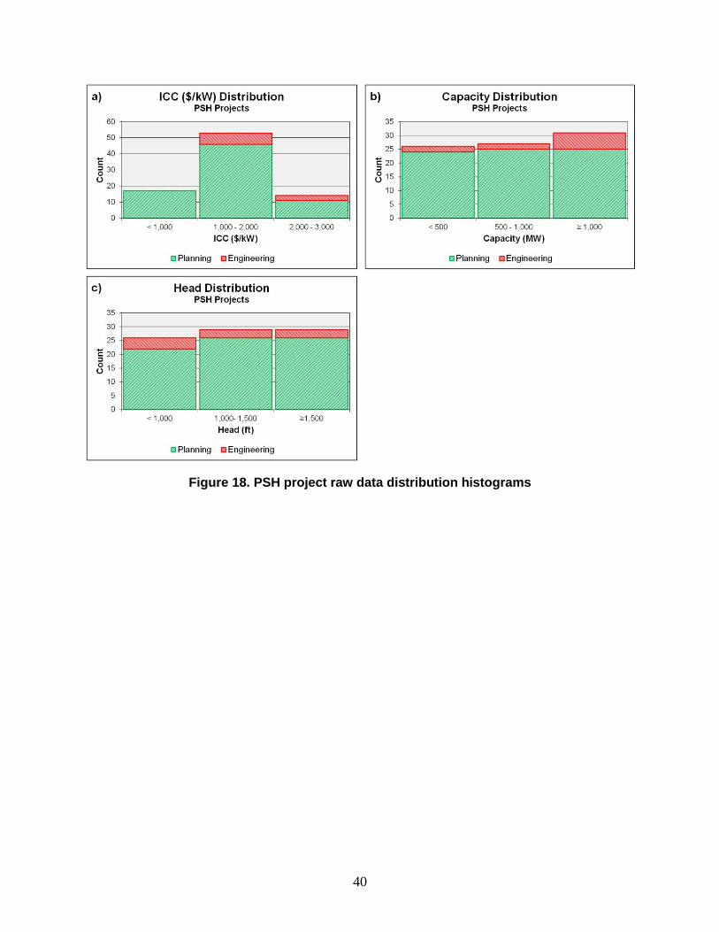
40
Figure 18. PSH project raw data distribution histograms
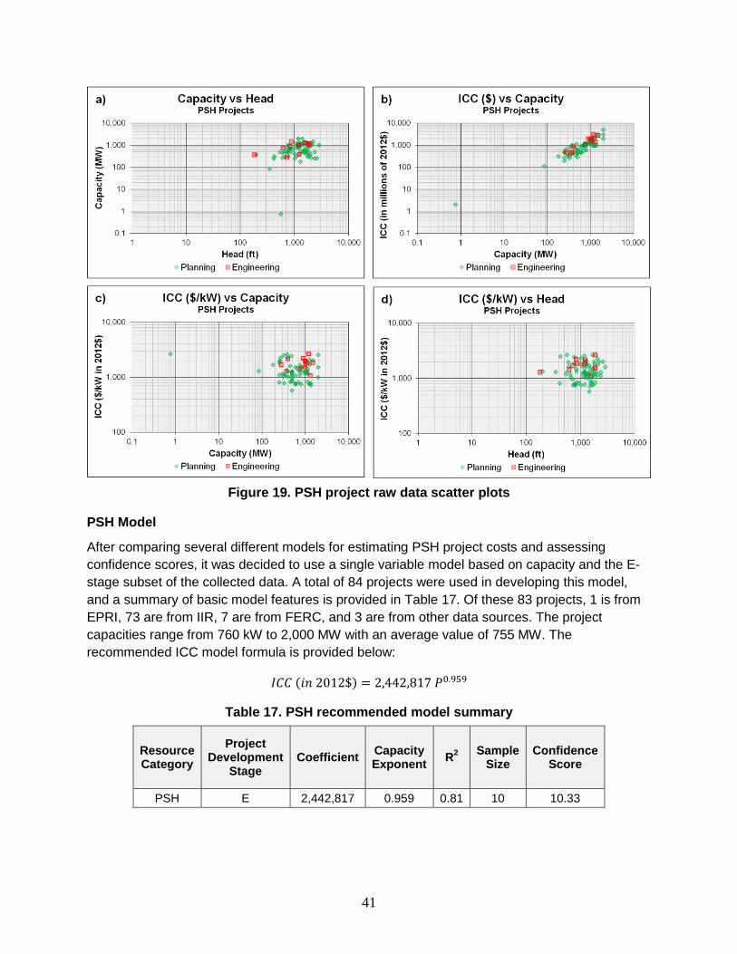
41
Figure 19. PSH project raw data scatter plots
PSH Model
After comparing several different models for estimating PSH project costs and assessing
confidence scores, it was decided to use a single variable model based on capacity and the E-
stage subset of the collected data. A total of 84 projects were used in developing this model,
and a summary of basic model features is provided in Table 17. Of these 83 projects, 1 is from
EPRI, 73 are from IIR, 7 are from FERC, and 3 are from other data sources. The project
capacities range from 760 kW to 2,000 MW with an average value of 755 MW. The
recommended ICC model formula is provided below:
𝐼𝐶𝐶 (𝑖𝑛 2012$) = 2,442,817 𝑃0.959
Table 17. PSH recommended model summary
Resource Category
Project Development
Stage Coefficient
Capacity Exponent
R2
Sample Size
Confidence Score
PSH E 2,442,817 0.959 0.81 10 10.33
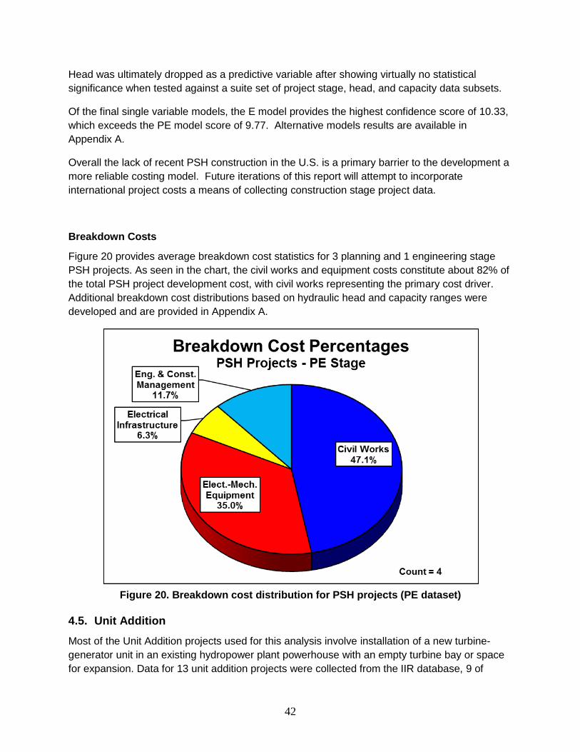
42
Head was ultimately dropped as a predictive variable after showing virtually no statistical
significance when tested against a suite set of project stage, head, and capacity data subsets.
Of the final single variable models, the E model provides the highest confidence score of 10.33,
which exceeds the PE model score of 9.77. Alternative models results are available in
Appendix A.
Overall the lack of recent PSH construction in the U.S. is a primary barrier to the development a
more reliable costing model. Future iterations of this report will attempt to incorporate
international project costs a means of collecting construction stage project data.
Breakdown Costs
Figure 20 provides average breakdown cost statistics for 3 planning and 1 engineering stage
PSH projects. As seen in the chart, the civil works and equipment costs constitute about 82% of
the total PSH project development cost, with civil works representing the primary cost driver.
Additional breakdown cost distributions based on hydraulic head and capacity ranges were
developed and are provided in Appendix A.
Figure 20. Breakdown cost distribution for PSH projects (PE dataset)
4.5. Unit Addition
Most of the Unit Addition projects used for this analysis involve installation of a new turbine-
generator unit in an existing hydropower plant powerhouse with an empty turbine bay or space
for expansion. Data for 13 unit addition projects were collected from the IIR database, 9 of
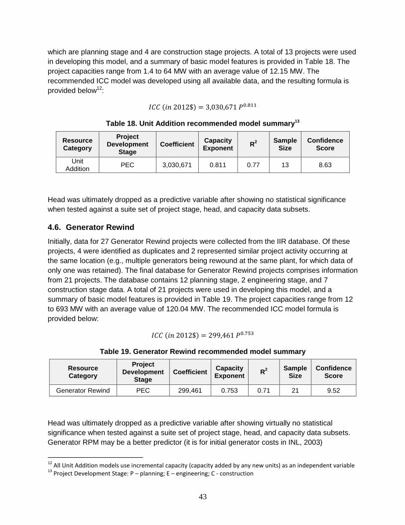
43
which are planning stage and 4 are construction stage projects. A total of 13 projects were used
in developing this model, and a summary of basic model features is provided in Table 18. The
project capacities range from 1.4 to 64 MW with an average value of 12.15 MW. The
recommended ICC model was developed using all available data, and the resulting formula is
provided below12:
𝐼𝐶𝐶 (𝑖𝑛 2012$) = 3,030,671 𝑃0.811
Table 18. Unit Addition recommended model summary13
Resource Category
Project Development
Stage Coefficient
Capacity Exponent
R2
Sample Size
Confidence Score
Unit Addition
PEC 3,030,671 0.811 0.77 13 8.63
Head was ultimately dropped as a predictive variable after showing no statistical significance
when tested against a suite set of project stage, head, and capacity data subsets.
4.6. Generator Rewind
Initially, data for 27 Generator Rewind projects were collected from the IIR database. Of these
projects, 4 were identified as duplicates and 2 represented similar project activity occurring at
the same location (e.g., multiple generators being rewound at the same plant, for which data of
only one was retained). The final database for Generator Rewind projects comprises information
from 21 projects. The database contains 12 planning stage, 2 engineering stage, and 7
construction stage data. A total of 21 projects were used in developing this model, and a
summary of basic model features is provided in Table 19. The project capacities range from 12
to 693 MW with an average value of 120.04 MW. The recommended ICC model formula is
provided below:
𝐼𝐶𝐶 (𝑖𝑛 2012$) = 299,461 𝑃0.753
Table 19. Generator Rewind recommended model summary
Resource Category
Project Development
Stage Coefficient
Capacity Exponent
R2
Sample Size
Confidence Score
Generator Rewind PEC 299,461 0.753 0.71 21 9.52
Head was ultimately dropped as a predictive variable after showing virtually no statistical
significance when tested against a suite set of project stage, head, and capacity data subsets.
Generator RPM may be a better predictor (it is for initial generator costs in INL, 2003)
12
All Unit Addition models use incremental capacity (capacity added by any new units) as an independent variable 13
Project Development Stage: P – planning; E – engineering; C - construction

44
4.7. Results Summary, Discussion, and Application
The recommended ICC model results for the six different resource categories are provided in
Table 20.
Table 20. Baseline cost model results by resource category
Resource Category Cost Model Equation
(ICC in 2012$; P in MW; H in ft)
Non-powered Dams 𝐼𝐶𝐶 = 12,038,038 𝑃0.980 𝐻−0.265
New Site Development projects 𝐼𝐶𝐶 = 8,717,830 𝑃0.975 𝐻−0.120
Canal/Conduit projects 𝐼𝐶𝐶 = 11,277,566 𝑃0.819 𝐻−0.177
Pumped Storage Hydropower projects 𝐼𝐶𝐶 = 2,442,817 𝑃0.959
Unit Addition projects 𝐼𝐶𝐶 = 3,030,671 𝑃0.811
Generator Rewind projects 𝐼𝐶𝐶 = 299,461𝑃0.753
Looking across the resources classes, the most notable was the unexpectedly weak economies
of scale associated with project capacity for the powering of non-powered dams and
development of new stream-reaches and pumped storage. In the NPD model a project twice the
size of another would only be 1.4% less expensive on $ per kW basis; this is similar for NSD
projects at 1.7%. While the economies of scale in pump storage development are marginally
higher—a doubling of capacity reduces costs by 2.9%--the difference in predicated cost
between the largest (2000 MW) and smallest (85 MW) projects in the dataset would only be
13.8%. And in many cases, the alternative models explored for each of these three resource
classes in Appendix A result in capacity exponents greater than 1, implying, contrary to
expectations, diseconomies of scale.
Previous studies have found strong economies of scale specifically in generating equipment
(INL, 2003; EPRI, 2011), which is supported by the findings with respect to unit additions and
generator rewinds. In light of this, the case may be that while equipment enjoys economy of
scale, the unique, site-specific nature of hydropower civil works “averages out” in the end, with
per kW costs minimally affected by the size of a project—at least for recent developments.
Additionally, the lack of head dependency for PSH, unit addition, and generator rewind projects
is surprising, but the data collected for these resource classes is the most scarce, and least
certain (as measured by amount C-stage data) of the 6 resources modeled. The PSH data also
mix projects with varying unique site attributes, such as existing upper or lower reservoirs or the
presence of other beneficial pre-existing infrastructure.
Ultimately, a model is only as good as the parts used to construct it, and the current versions of
the BCM models would benefit substantially from improvements in data availability, cost
uniformity, and validation. As described in previous sections, the majority of the cost data
available for this effort are from early planning and engineering stage. Ideally, more data would
be available to enhance raw cost accuracy, and the confidence scoring methodology attempts
to address this concern. In the end, exploring additional avenues for obtaining quality cost data

45
is of primary importance to ORNL’s cost modeling efforts and may be achieved through
significant industry collaboration.
In spite of these limitations and opportunities for improvement, the models developed in this
report can be used to assess the relative economics of remaining U.S. hydropower resources.
Figure 21 below compares the historical LCOEs introduced in Section 2.4 to the LCOE of NPD
(from Hadjerioua et. al., 2012)14 and NSD (from Kao et. al., 2014) resources greater than 1 MW
in size available in the U.S. when their costs are estimated using the new models15. Boxes
represent the spread between 25th and 75th percentiles and whiskers are the furthest points
within 1.5 times the interquartile range
Figure 21 - Application of NSD and NPD BCMs to U.S. undeveloped resources > 1 MW
14
The costs in Figure 21 are based on dams identified in Hadjerioua et al. (2012) but the sizing and annual generation forecasts for the hydropower plants have been modified according to the NSD methodology in Kao et. al. (2014). 15
An availability of factors of 93% is applied to the resource assessment raw generation potential for consistency with the hydropower assumptions in DOE (2012) and NREL (2012), derived from historical NERC GADS reporting.
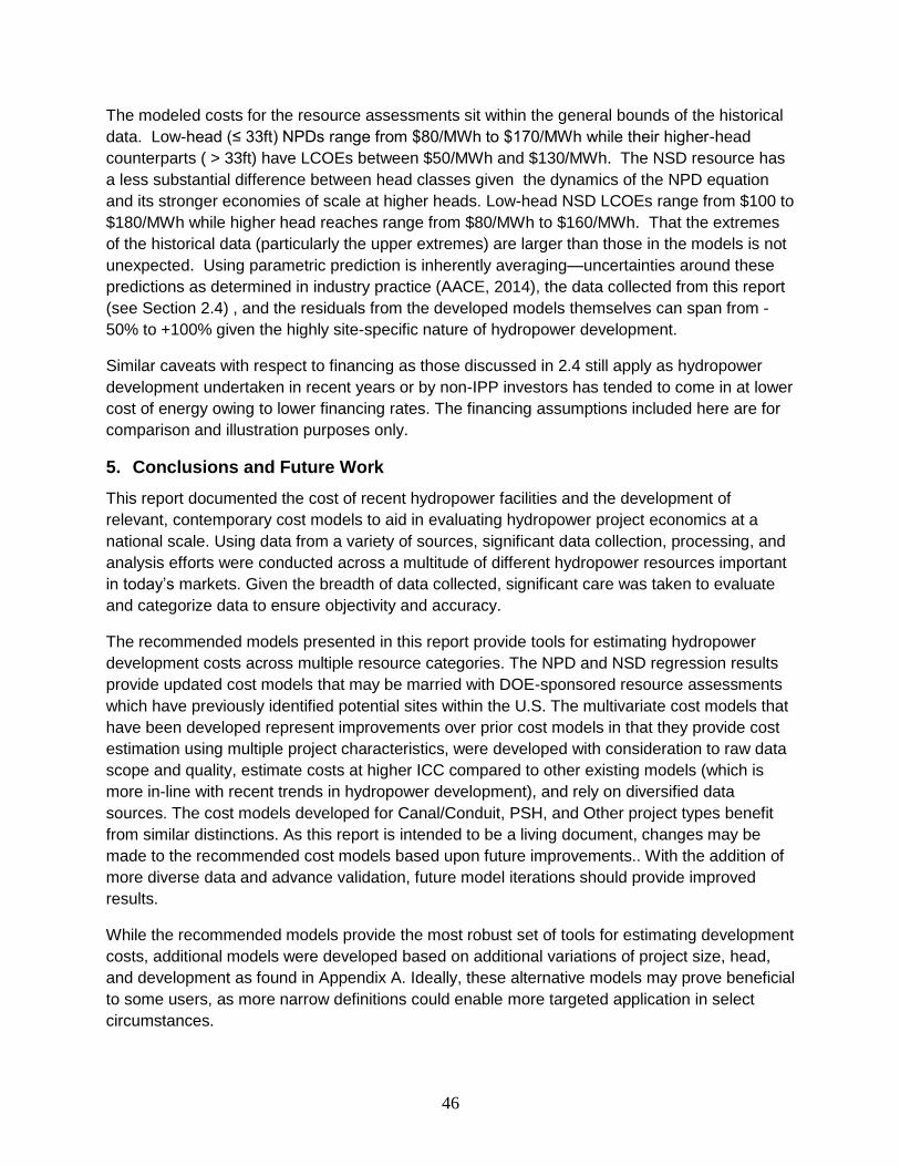
46
The modeled costs for the resource assessments sit within the general bounds of the historical
data. Low-head (≤ 33ft) NPDs range from $80/MWh to $170/MWh while their higher-head
counterparts ( > 33ft) have LCOEs between $50/MWh and $130/MWh. The NSD resource has
a less substantial difference between head classes given the dynamics of the NPD equation
and its stronger economies of scale at higher heads. Low-head NSD LCOEs range from $100 to
$180/MWh while higher head reaches range from $80/MWh to $160/MWh. That the extremes
of the historical data (particularly the upper extremes) are larger than those in the models is not
unexpected. Using parametric prediction is inherently averaging—uncertainties around these
predictions as determined in industry practice (AACE, 2014), the data collected from this report
(see Section 2.4) , and the residuals from the developed models themselves can span from -
50% to +100% given the highly site-specific nature of hydropower development.
Similar caveats with respect to financing as those discussed in 2.4 still apply as hydropower
development undertaken in recent years or by non-IPP investors has tended to come in at lower
cost of energy owing to lower financing rates. The financing assumptions included here are for
comparison and illustration purposes only.
5. Conclusions and Future Work
This report documented the cost of recent hydropower facilities and the development of
relevant, contemporary cost models to aid in evaluating hydropower project economics at a
national scale. Using data from a variety of sources, significant data collection, processing, and
analysis efforts were conducted across a multitude of different hydropower resources important
in today’s markets. Given the breadth of data collected, significant care was taken to evaluate
and categorize data to ensure objectivity and accuracy.
The recommended models presented in this report provide tools for estimating hydropower
development costs across multiple resource categories. The NPD and NSD regression results
provide updated cost models that may be married with DOE-sponsored resource assessments
which have previously identified potential sites within the U.S. The multivariate cost models that
have been developed represent improvements over prior cost models in that they provide cost
estimation using multiple project characteristics, were developed with consideration to raw data
scope and quality, estimate costs at higher ICC compared to other existing models (which is
more in-line with recent trends in hydropower development), and rely on diversified data
sources. The cost models developed for Canal/Conduit, PSH, and Other project types benefit
from similar distinctions. As this report is intended to be a living document, changes may be
made to the recommended cost models based upon future improvements.. With the addition of
more diverse data and advance validation, future model iterations should provide improved
results.
While the recommended models provide the most robust set of tools for estimating development
costs, additional models were developed based on additional variations of project size, head,
and development as found in Appendix A. Ideally, these alternative models may prove beneficial
to some users, as more narrow definitions could enable more targeted application in select
circumstances.

47
For all of the models presented, consideration should be made to limitations related to raw data
breadth, and attempts have been made to identify such limitations. One key limitation to the
models presented in this report is the lack of estimating tools for operations and maintenance,
licensing and permitting, and explicit costing of environmental mitigation technologies. Work to
fill these gaps is ongoing, but for immediate practical application, historical models such as
those developed in INL (2003) are recommended. Additionally, future iterations of the report will
include the collection of more robust component cost data that will form the basis of “typical
plant” cost profiles demonstrating the distribution of costs within a project.

48
References
AACE (2013). Cost Estimate Classification System – As Applied in Engineering, Procurement,
and Construction for the Hydropower Industry. AACE International Recommended Practice No.
69R-12. January, 2013.
BLS (Bureau of Labor Statistics) (2014). Producer Price Indexes, available online at http://www.bls.gov/ppi/, accessed online September 2014.
Butterfield, S. (2011). Presentation on Swalley Irrigation District’s Ponderosa Hydroelectric Project during the Deschutes River Basin Site Visit. Swalley Irrigation District, June 1, 2011.
City of Boulder (2013), City of Boulder Hydroelectric Facility Summary Sheet, available at https://www-static.bouldercolorado.gov/docs/Agenda_5_-_Hydroelectric_Program_Update-1-201307111316.pdf, accessed online March 2014.
COID (Central Oregon Irrigation District) and ODE (Oregon Department of Energy) (2011). Feasibility Study for Six Central Oregon Irrigation District Potential Hydroelectric Power Generation Sites, Oregon.
Cotchen, D. (2014). PECTRAX – Project Activity Flow Chart, Industrial Info Resources, Written Communications.
DOE (Department of Energy) and, EPRI (Electric Power Research Institute) (1985a). Small-Hydropower Development: The Process, Pitfalls, and Experience Volume 1: Feasibility Studies Summary and Analysis, EPRI EM-4036.
DOE (Department of Energy) and EPRI (Electric Power Research Institute) (1985b). Small-Hydropower Development: The Process, Pitfalls, and Experience Volume 2: Licensing Activities Summary and Analysis, EPRI EM-4036.
DOE (Department of Energy) and EPRI (Electric Power Research Institute) (1986). Small-Hydropower Development: The Process, Pitfalls, and Experience Volume 4: Guide for Developers, EPRI EM-4036.
DOE (Department of Energy) and, EPRI (Electric Power Research Institute) (1987). Small-Hydropower Development: The Process, Pitfalls, and Experience Volume 3: Summary and Analysis of Technology Development Projects, EPRI EM-4036.
DOE (Department of Energy) (2012). SunShot Vision Study, NREL Report No. BK-5200-47927, DOE/GO-102012-3037, Washington DC.
DOE (Department of Energy) (2014). Presentation on Recovery Act: Hydroelectric Facility Modernization Project, accessed on February, 2014.
Duan, N. (1983). Smearing Estimate: A Nonparametric retransformation Method, J. of the American Statistical Association, 78(383), 605-610.
49
EIA (Energy Information Administration) (2013). Updated Capital Cost Estimates for Utility Scale Electricity Generating Plants, available at http://www.eia.gov/forecasts/capitalcost/pdf/updated_capcost.pdf, accessed online January 2014.
EIA (Energy Information Administration) (2014a). Nonhydro Renewable Now Routinely Surpass Hydropower Generation, available at http://www.eia.gov/todayinenergy/, accessed online August 2014.
EIA (Energy Information Administration) (2014b). Annual Energy Outlook 2014: with Projections to 2040, DOE/EIA-0383(2014). Washington, DC.
ENR (Engineering News Record) (2013). Construction Cost Indices, Engineering News Record,
available online at http://enr.construction.com/economics/, accessed online June 2013.
EPRI (2011) Quantifying the Value of Hydropower in the Electric Grid: Plant Cost Elements.
EPRI, Palo Alto, CA: 2011. 1023140.
ETO (Energy Trust of Oregon) (2010). Irrigation Water Providers of Oregon: Hydropower
Potential and Energy Savings Evaluation, Oregon.
FERC (Federal Energy Regulatory Commission) (2014). Federal Energy Regulatory Commission, available at http://www.ferc.gov/, accessed online January 2014.
FHWA (Federal Highway Administration) (2014). Price Trends for Federal-Aid Highway
Construction, available online at http://fhwa.dot.gov, accessed online September 2014.
Gordon, J.L. and Penman, A.C. (1979). Quick Estimating Techniques for Small Hydro Potential, J. of Power Dam Constr., 31 (1979) pp.46-55.
Hadjerioua, B., Wei, Y., and Kao, S.C. (2012). An Assessment of Energy Potential at Non-powered Dams in the United States, GPO DOE/EE-0711, Wind and Water Power Program, Department of Energy, DC.
IIR (Industrial Info Resources) (2014). PECWeb – A Searchable Database, available at http://www.industrialinfo.com/database , accessed online March 2014.
INL (Idaho National Lab) (2003). Estimation of Economic Parameters of U.S. Hydropower Resources, INEEL/EXT-03-00662.
Kao, S.C., McManamay, R.A., Stewart, K.M., Samu, N.M., Hadjerioua, B., DeNeale, S.T., Yeasmin, D., Pasha, M.F. K., Oubeidillah, A.A., and Smith, B.T. (2014). New Stream-reach Development: A Comprehensive Assessment of Hydropower Energy Potential in the United States, GPO DOE/EE-1063, Wind and Water Power Program, Department of Energy, Washington, DC.
Newman, M.C. (1993). Regression Analysis of Log-transformed Data: Statistical Bias and its Correction, Environmental Toxicology and Chemistry, vol. 12, 1129-1133.
NHAAP (National Hydropower Asset Assessment Program) (2014). Oak Ridge National Laboratory, available at http://nhaap.ornl.gov/, accessed online June 2014.

50
NREL (National Renewable Energy Laboratory) (2012). Renewable Electricity Futures Study, 4 vols. NREL/TP-6A20-52409, Golden, Colorado.
NUID (North Unit Irrigation District) (2009). Feasibility Study on Five Potential Hydroelectric Power Generation Locations in the North Unit Irrigation District, Oregon, August 2009.
OpenEI (Open Energy Forum) (2014). Transparent Cost Database, available at http://en.openei.org/wiki/Transparent_Cost_Database, accessed online August 2014.
Remer, D., Lin, S., Yu, N., and Hsin, K. (2008). An Update on Cost and Scale-up Factors, International Inflation, Int. J. Production Economics, 333-346.
RSMeans (2013). Historical Cost Indices, RSMeans, available online at
http://www.rsmeansonline.com, accessed online June 2013.
TVA (Tennessee Valley Authority) (1941). The Guntersville Project: A Comprehensive Report on the Planning, Design, Construction, and Initial Operations of the Guntersville Project, Technical Report No. 4, Knoxville, Tennessee.
USACE (United States Army Corps of Engineers) and MWH (2009). Technical Analysis of Pumped Storage and Integration with Wind Power in the Pacific Northwest. MWH Prepared for U.S. Army Corps of Engineers, Northwest Division, Hydroelectric Design Center.
USACE (United States Army Corps of Engineers) (2013a). Civil Works Construction Cost Index System, Army Corps of Engineers, available online at http://www.nww.usace.army.mil/Missions/CostEngineering.aspx, accessed online June 2013.
USACE (United States Army Corps of Engineers) (2013b). Hydropower Resource Assessment At Non-Powered USACE Sites.
USBR (United States Bureau of Reclamation) (1988). Spring Canyon Pumped Storage Project, Bureau of Reclamation, Lower Colorado Region, Boulder City, Nevada, October 1988.
USBR (United States Bureau of Reclamation) (2013). Hydropower Construction Costs Trends, Bureau of Reclamation, available online at http://www.usbr.gov/pmts/estimate/cost_trend.html, accessed online June 2013.
Xiao, X., White, E.P., Hooten, M.B., and Durham, S.L. (2011). On the use of Log-
Transformation vs. Nonlinear Regression for Analyzing Biological Power Laws, Ecology 92,
1887-1894.
Zhang, Q.F., Smith, B., and Zhang, W. (2012). Small Hydropower Cost Reference Model,
ORNL/TM-2012/501.

51

A-1
Appendix A – Alternative Models, Detailed Comparison, and Validation

A-2
Raw Data
The previous discussion on raw data illustrates the primary data sources for each resource but
provides no comparison on the overall raw data. Figure 22 shows statistical distribution of cost
data, providing the number of projects in each resource category, along with the average ICC.
As shown in the Figure 22, NSD, NPD, and Canal/Conduit projects tend to have the highest per
kW development costs, while the plant overhaul-related projects tend to be much lower cost. As
the plot is shown on a logarithmic scale, the magnitude of cost variation is somewhat skewed.
With careful thought, one can see that certain types of projects (NPDs for instance) contain
relatively high variability, while others (such as PSH) are relatively consistent in terms of cost.
A total of 600 projects were used for the final analysis. 575 out of 600 projects were located in
the U.S. with the remaining 25 projects from Non-US. As shown in the Figure 23 map, the
United States was divided into six market regions: Southwest, Midwest, Rocky Mountains,
Pacific, Southeast, and Northeast.
For each of the resource categories, Appendix A provides information on regional cost data
distributions, alternative models, in-sample model validation, and breakdown cost distributions.
The regional raw cost data distribution diagram provides statistics on the U.S. (six regions) and
Non-US data. However, the discussion on raw cost data are focused on the U.S. regions only.
Alternative models which were developed based on project development stage, installed
capacity and hydraulic head ranges are documented. The raw costs vs. model estimated costs
are compared using in-sample validation plots. The breakdown costs are categorized into 4
different components, including= 1) Civil Works 2) Electro Mechanical Equipment 3) Electrical
infrastructure, and 4) Engineering & Construction Management. Only those projects having cost
data for all four components are included in the analysis.
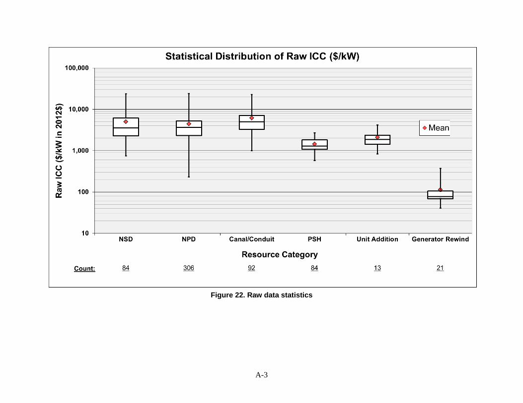
A-3
Figure 22. Raw data statistics

A-4
Figure 23. Regional classification of the United States

A-5
Non-powered Dams
The previous discussion on NPD data illustrates the primary data sources but provides no
details on the project locations included. As shown in the Figure 23 map, the United States was
divided into six market regions: Southwest, Midwest, Rocky Mountains, Pacific, Southeast, and
Northeast. Figure 24 shows regional distribution of cost data, providing the number of NPD
projects in each region, along with the average ICC, capacity, and hydraulic head. A total of
306 NPDs projects were used for the final analysis. 302 out of 306 projects were located in the
U.S. with the remaining 4 projects from Non-US. A minimum of 10 projects were located in the
Southwest region, while a maximum of 79 projects were located in the Northeast region.
Cumulative regional project capacity ranges from 84 MW in the Southwest to 1,565 MW in the
Southeast, while regionally-averaged hydraulic head ranges from 27 ft in the Midwest to 254 ft
in the Rocky Mountains region. The ICC varies significantly among the regions, with a minimum
of 2,788 $/kW in the Southwest and a maximum of 5,725 $/kW in the Midwest.
As described in Section 4 of this report, the recommended cost model for NPD ICC estimation is
the C Dataset model, which used construction stage project data only. However, numerous
other models were evaluated as a part of the BCM development efforts. Table 21 provides
various statistics for multiple models that were developed. Correlation and regression results
are provided to help inform users of the relative benefits and limitations of using alternative NPD
models.
Figure 25 shows multiple in-sample validation plots that demonstrate the results for the PEC,
EC, and C models for NPDs. The top plots (Figure 25a-c) show modeled vs. raw ICC for each
model. The diagonal 1:1 line represents where the modeled and raw costs are equal and is the
ideal case for estimating cost using a model. The bottom plots (Figure 25d-f) show raw and
modeled cost data relative to the combined capacity and head power forms. The blue points
represent raw cost, while the black diagonal line represents modeled ICC. The red diagonal
lines represent the upper and lower 95% confidence interval ICC. Ideally, all raw data would lie
within the confidence interval, though sample size, correlation, and other factors influence the
results.
Figure 26 shows NPD breakdown cost distributions across a variety of different capacity ranges.
These breakdown costs are categorized into 4 different groups according to the major sources
of development cost. As seen in the plots, the major cost drivers for NPDs are civil works and
equipment costs. For the smaller projects (below 1 MW), equipment costs are significantly high
(nearly 50% on average). Though Civil Works constitute an incrementally higher portion of total
ICC for projects above 1 MW, equipment cost remains higher than the Civil Works for all
capacity ranges evaluated. For the larger projects (above 30 MW), engineering and construction
management costs are relatively minor, as the overall scope involved in such activities remains
similar between large and small projects. Since consideration should be given to the number of
projects from which these plots were made, the project count is provided in the lower corner of
each plot.

A-6
Similarly, Figure 27 shows breakdown cost distributions for NPDs across various head ranges.
The low head projects (below 30 ft) demonstrate high equipment cost contribution. High head
projects, on the other hand, show similar equipment and civil works cost percentages.
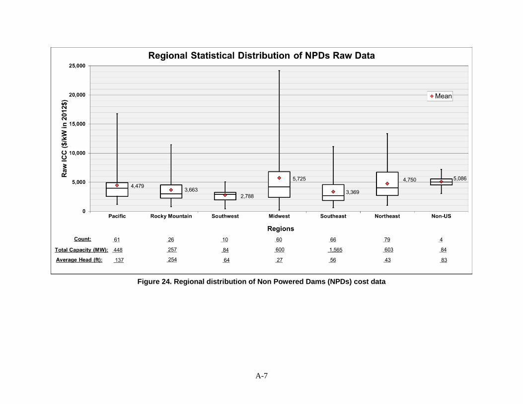
A-7
Figure 24. Regional distribution of Non Powered Dams (NPDs) cost data

A-8
Table 21. Summary regression results for NPDs
Category
Model Estimated Cost
(in 2012$) R
2
Sample
Size
Confidence
Score
Bias
Correction
Coefficien
t log
(Intercept)
Coefficien
t log
(Capacity)
Coefficient
log
(Head)
t - statistic value p - value
Log
(Constant) log(P) log(H)
Log
(Constant) log(P) log(H)
Modeling Results by Project Development Stage
All data (PEC) 9,723,751 P0.77 H-0.13 0.80 306 9.18 1.16 15.94 0.77 -0.13 129.69 34.9 -4.1 1.65E-267 3.9E-108 5.5E-05
Eng. &
Construction 8,279,590 P0.94 H-0.16 0.90 80 12.35 1.09 15.84 0.94 -0.16 79.41 26.9 -3.3 1.25E-75 7.1E-41 1.6E-03
Construction 12,038,038 P0.98 H-0.27 0.92 28 13.34 1.06 16.24 0.98 -0.27 50.50 16.7 -4.0 1.10E-26 4.4E-15 4.6E-04
Modeling Results by Project Capacity (MW)
< 1 MW 16,806,429 P0.95 H-0.23 0.64 44 1.14 16.50 0.95 -0.23 50.68 8.5 -3.0 1.31E-38 1.6E-10 4.6E-03
1 to < 10 MW 10,461,047 P0.76 H-0.15 0.51 157 1.10 16.07 0.76 -0.15 93.42 12.1 -4.1 1.65E-137 4.9E-24 6.0E-05
10 to < 30 MW 7,688,334 P0.71 H-0.01 0.10 77 1.26 15.63 0.71 -0.01 23.36 2.9 -0.1 1.65E-137 4.5E-03 8.9E-01
≥ 30 MW 33,301,325 P0.64 H-0.29 0.30 28 1.19 17.15 0.64 -0.29 14.25 2.4 -2.1 6.91E-36 2.3E-02 4.6E-02
Modeling Results by Head (ft)
< 30 ft 7,779,007 P0.76 H-0.02 0.81 121 1.18 15.70 0.76 -0.02 39.41 21.5 -0.1 9.28E-70 1.5E-42 9.1E-01
30 to < 67 ft 9,673,784 P0.79 H-0.16 0.81 83 1.16 15.94 0.79 -0.16 16.81 18.3 -0.6 5.52E-28 2.5E-30 5.2E-01
< 67 ft 12,680,066 P0.78 H-0.22 0.81 204 1.17 16.20 0.78 -0.22 72.30 28.9 -3.1 7.80E-146 1.5E-73 2.2E-03
67 to< 200 ft 11,071,568 P0.7 H-0.13 0.75 79 1.14 16.09 0.70 -0.13 20.28 15.0 -0.8 2.18E-32 2.4E-24 4.3E-01
≥ 200 ft 9,010,765 P0.85 H-0.14 0.90 23 1.07 15.94 0.85 -0.14 16.20 12.2 -0.9 5.75E-13 9.6E-11 4.0E-01
Note: the model estimated cost includes bias correction.

A-9
Figure 25. NPD in-sample model validation
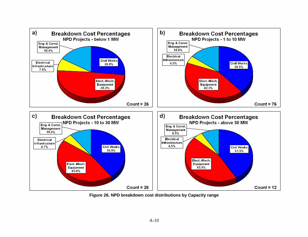
A-10
Figure 26. NPD breakdown cost distributions by Capacity range
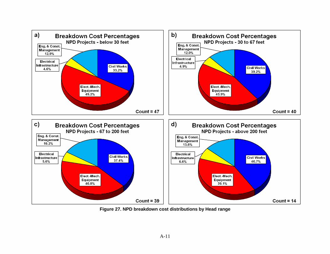
A-11
Figure 27. NPD breakdown cost distributions by Head range

A-12
New Stream-reach Developments (NSDs)
The previous discussion on NSD data illustrates the primary data sources but provides no
details on the project locations included. As shown in the Figure 23 map, the United States was
divided into six market regions: Southwest, Midwest, Rocky Mountains, Pacific, Southeast, and
Northeast. Figure 28 shows regional distribution of cost data, providing the number of NSD
projects in each region, along with the average ICC, capacity, and hydraulic head. A total of 84
NSD projects were used for the final analysis. 63 out of 84 projects were located in the U.S.
with the remaining 21 projects from Non-US. No project data were available for the Southwest
region. A minimum of 5 projects were located in the Midwest region, while a maximum of 34
projects were located in the Pacific region. The cumulative regional project capacity ranges from
2 MW in the Midwest to 1,555 MW in the Pacific, while the regionally-averaged hydraulic head
ranges from 14 ft in the Midwest to 838 ft in the Pacific. The ICC varies significantly among the
regions, 3,573 $/kW in the Pacific to 18,425 $/kW in the Midwest.
As described in Section 4 of this report, the recommended cost model for NSD ICC estimation is
the C Dataset model, which used construction stage project data only. However, numerous
other models were evaluated as a part of the BCM development efforts. Table 22 provides
various statistics for multiple models that were developed. Correlation and regression results
are provided to help inform users of the relative benefits and limitations of using alternative NSD
models.
Figure 29 shows multiple in-sample validation plots that demonstrate the results for the PEC,
EC, and C models for NSDs. The top plots (Figure 29a-c) show modeled vs. raw ICC for each
model. The diagonal 1:1 line represents where the modeled and raw costs are equal and is the
ideal case for estimating cost using a model. The bottom plots (Figure 29d-f) show raw and
modeled cost data relative to the combined capacity and head power forms. The blue points
represent raw cost, while the black diagonal line represents modeled ICC. The red diagonal
lines represent the upper and lower 95% confidence interval ICC. Ideally, all raw data would lie
within the confidence interval, though sample size, correlation, and other factors influence the
results.
Figure 30 shows NSD breakdown cost distributions across a variety of different capacity ranges.
These breakdown costs are categorized into 4 different groups according to the major source of
development cost. As seen in the plots, the major cost drivers for NSDs are civil works and
equipment costs. For the smaller projects (below 1 MW), equipment costs are significantly high
(nearly 55% on average); however, for larger projects (above 30 MW), civil works contribute
more to overall ICC (nearly 47% on average) due to construction of a new dam or diversion
structure and waterway facilities. The engineering & construction management costs are
relatively minor for all projects. Since consideration should be given to the number of projects
from which these plots were made, the project count is provided in the lower corner of each plot.
Similarly, Figure 31 shows breakdown cost distributions for NSDs across various head ranges.
The low head projects (below 67 ft) as well as high head (above 200 ft) demonstrate high civil
works cost contribution. The equipment cost contribution remains similar for both low and high

A-13
head projects. The breakdown cost distribution for medium head (67 to 200 ft) NSD projects is
not provided due to unavailability of the data.
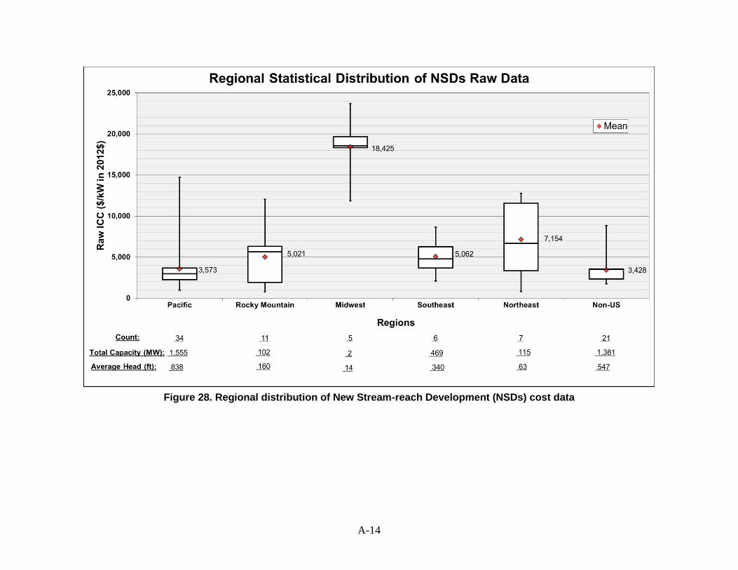
A-14
Figure 28. Regional distribution of New Stream-reach Development (NSDs) cost data
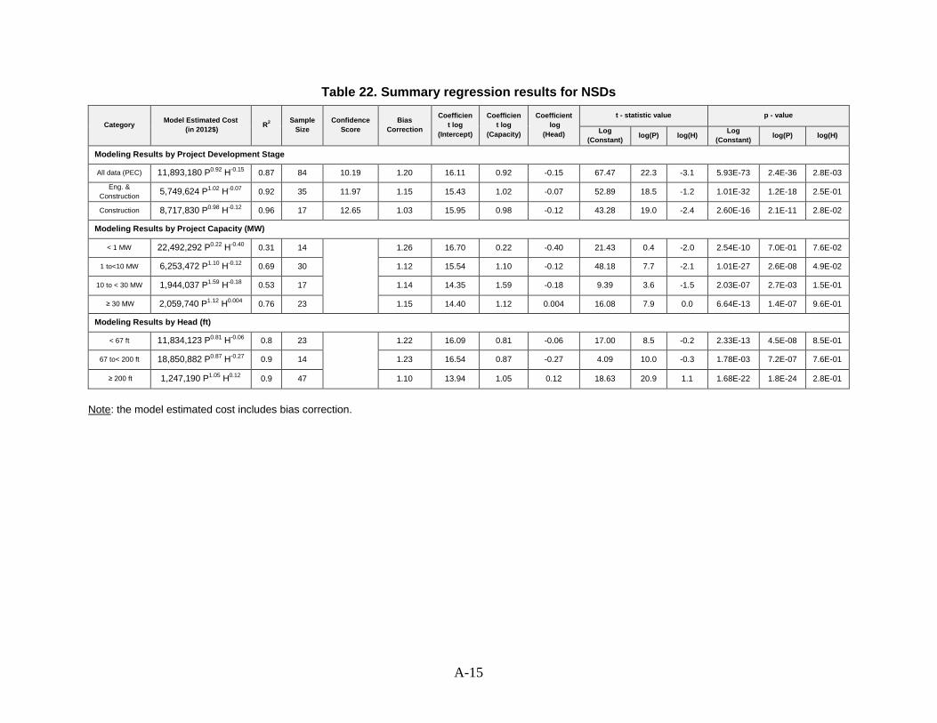
A-15
Table 22. Summary regression results for NSDs
Category
Model Estimated Cost
(in 2012$) R
2
Sample
Size
Confidence
Score
Bias
Correction
Coefficien
t log
(Intercept)
Coefficien
t log
(Capacity)
Coefficient
log
(Head)
t - statistic value p - value
Log
(Constant) log(P) log(H)
Log
(Constant) log(P) log(H)
Modeling Results by Project Development Stage
All data (PEC) 11,893,180 P0.92 H-0.15 0.87 84 10.19 1.20 16.11 0.92 -0.15 67.47 22.3 -3.1 5.93E-73 2.4E-36 2.8E-03
Eng. &
Construction 5,749,624 P1.02 H-0.07 0.92 35 11.97 1.15 15.43 1.02 -0.07 52.89 18.5 -1.2 1.01E-32 1.2E-18 2.5E-01
Construction 8,717,830 P0.98 H-0.12 0.96 17 12.65 1.03 15.95 0.98 -0.12 43.28 19.0 -2.4 2.60E-16 2.1E-11 2.8E-02
Modeling Results by Project Capacity (MW)
< 1 MW 22,492,292 P0.22 H-0.40 0.31 14 1.26 16.70 0.22 -0.40 21.43 0.4 -2.0 2.54E-10 7.0E-01 7.6E-02
1 to<10 MW 6,253,472 P1.10 H-0.12 0.69 30 1.12 15.54 1.10 -0.12 48.18 7.7 -2.1 1.01E-27 2.6E-08 4.9E-02
10 to < 30 MW 1,944,037 P1.59 H-0.18 0.53 17 1.14 14.35 1.59 -0.18 9.39 3.6 -1.5 2.03E-07 2.7E-03 1.5E-01
≥ 30 MW 2,059,740 P1.12 H0.004 0.76 23 1.15 14.40 1.12 0.004 16.08 7.9 0.0 6.64E-13 1.4E-07 9.6E-01
Modeling Results by Head (ft)
< 67 ft 11,834,123 P0.81 H-0.06 0.8 23 1.22 16.09 0.81 -0.06 17.00 8.5 -0.2 2.33E-13 4.5E-08 8.5E-01
67 to< 200 ft 18,850,882 P0.87 H-0.27 0.9 14 1.23 16.54 0.87 -0.27 4.09 10.0 -0.3 1.78E-03 7.2E-07 7.6E-01
≥ 200 ft 1,247,190 P1.05 H0.12 0.9 47 1.10 13.94 1.05 0.12 18.63 20.9 1.1 1.68E-22 1.8E-24 2.8E-01
Note: the model estimated cost includes bias correction.
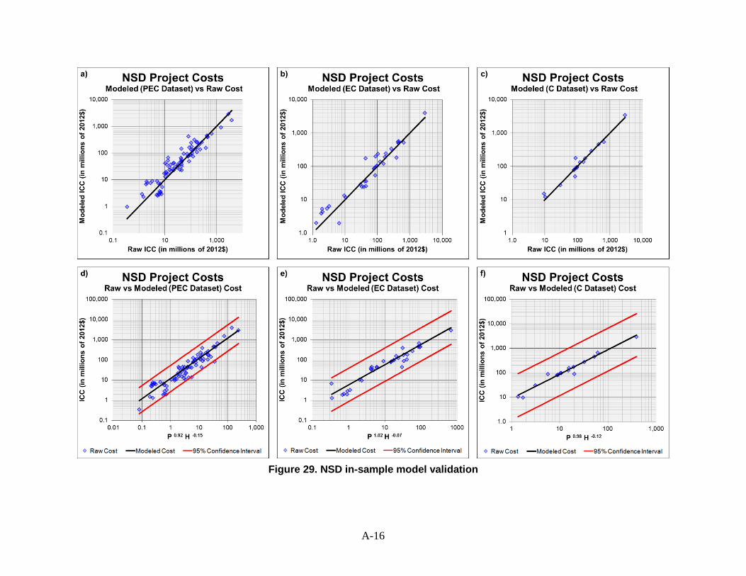
A-16
Figure 29. NSD in-sample model validation

A-17
Figure 30. NSD breakdown cost distributions by Capacity range
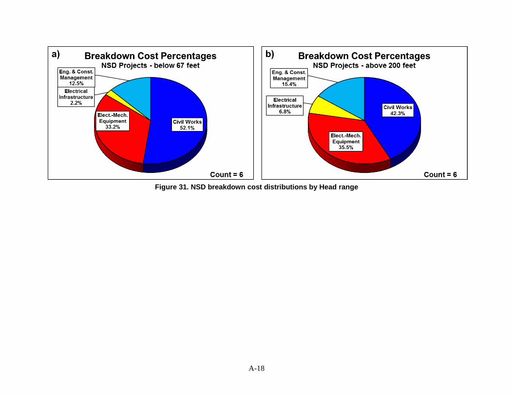
A-18
Figure 31. NSD breakdown cost distributions by Head range
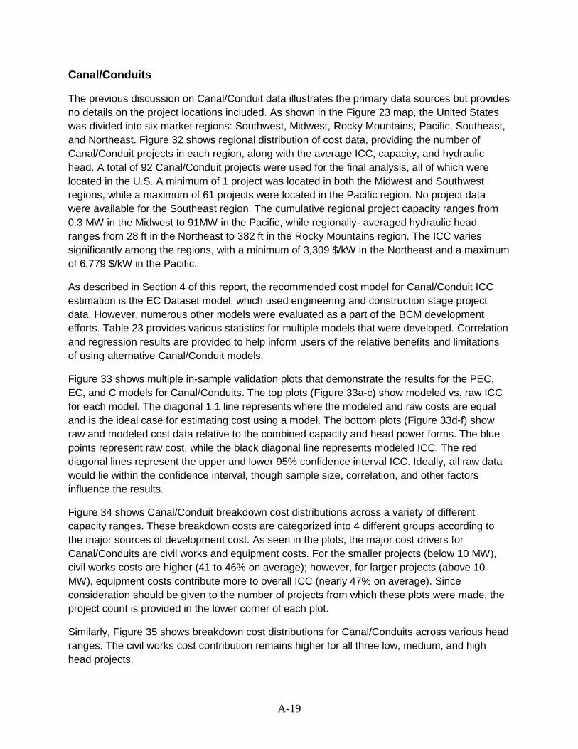
A-19
Canal/Conduits
The previous discussion on Canal/Conduit data illustrates the primary data sources but provides
no details on the project locations included. As shown in the Figure 23 map, the United States
was divided into six market regions: Southwest, Midwest, Rocky Mountains, Pacific, Southeast,
and Northeast. Figure 32 shows regional distribution of cost data, providing the number of
Canal/Conduit projects in each region, along with the average ICC, capacity, and hydraulic
head. A total of 92 Canal/Conduit projects were used for the final analysis, all of which were
located in the U.S. A minimum of 1 project was located in both the Midwest and Southwest
regions, while a maximum of 61 projects were located in the Pacific region. No project data
were available for the Southeast region. The cumulative regional project capacity ranges from
0.3 MW in the Midwest to 91MW in the Pacific, while regionally- averaged hydraulic head
ranges from 28 ft in the Northeast to 382 ft in the Rocky Mountains region. The ICC varies
significantly among the regions, with a minimum of 3,309 $/kW in the Northeast and a maximum
of 6,779 $/kW in the Pacific.
As described in Section 4 of this report, the recommended cost model for Canal/Conduit ICC
estimation is the EC Dataset model, which used engineering and construction stage project
data. However, numerous other models were evaluated as a part of the BCM development
efforts. Table 23 provides various statistics for multiple models that were developed. Correlation
and regression results are provided to help inform users of the relative benefits and limitations
of using alternative Canal/Conduit models.
Figure 33 shows multiple in-sample validation plots that demonstrate the results for the PEC,
EC, and C models for Canal/Conduits. The top plots (Figure 33a-c) show modeled vs. raw ICC
for each model. The diagonal 1:1 line represents where the modeled and raw costs are equal
and is the ideal case for estimating cost using a model. The bottom plots (Figure 33d-f) show
raw and modeled cost data relative to the combined capacity and head power forms. The blue
points represent raw cost, while the black diagonal line represents modeled ICC. The red
diagonal lines represent the upper and lower 95% confidence interval ICC. Ideally, all raw data
would lie within the confidence interval, though sample size, correlation, and other factors
influence the results.
Figure 34 shows Canal/Conduit breakdown cost distributions across a variety of different
capacity ranges. These breakdown costs are categorized into 4 different groups according to
the major sources of development cost. As seen in the plots, the major cost drivers for
Canal/Conduits are civil works and equipment costs. For the smaller projects (below 10 MW),
civil works costs are higher (41 to 46% on average); however, for larger projects (above 10
MW), equipment costs contribute more to overall ICC (nearly 47% on average). Since
consideration should be given to the number of projects from which these plots were made, the
project count is provided in the lower corner of each plot.
Similarly, Figure 35 shows breakdown cost distributions for Canal/Conduits across various head
ranges. The civil works cost contribution remains higher for all three low, medium, and high
head projects.
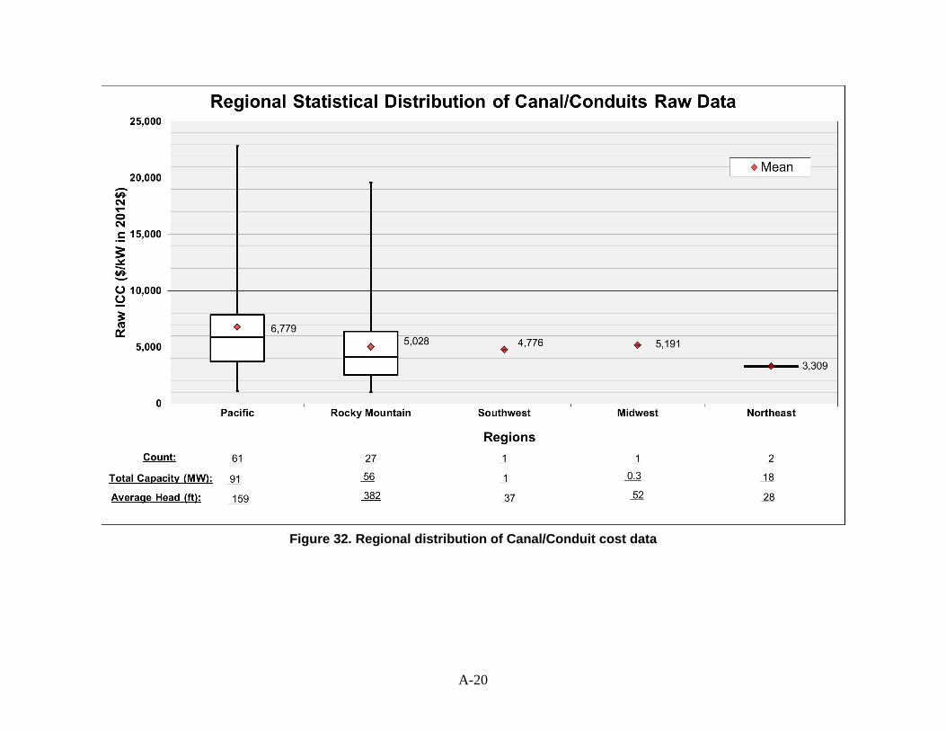
A-20
Figure 32. Regional distribution of Canal/Conduit cost data
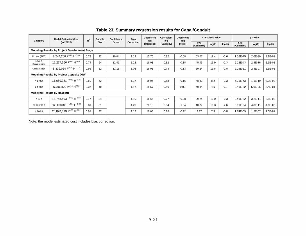
A-21
Table 23. Summary regression results for Canal/Conduit
Category
Model Estimated Cost
(in 2012$) R
2
Sample
Size
Confidence
Score
Bias
Correction
Coefficient
log
(Intercept)
Coefficient
log
(Capacity)
Coefficient
log
(Head)
t - statistic value p - value
Log
(Constant) log(P) log(H)
Log
(Constant) log(P) log(H)
Modeling Results by Project Development Stage
All data (PEC) 8,244,256 P0.82 H-0.08 0.78 92 10.04 1.19 15.75 0.82 -0.08 63.07 17.4 -1.6 1.16E-75 2.0E-30 1.1E-01
Eng. &
Construction 11,277,566 P0.82 H-0.18 0.74 54 12.41 1.23 16.03 0.82 -0.18 45.45 11.9 -2.3 6.13E-43 2.3E-16 2.3E-02
Construction 8,339,054 P0.74 H-0.13 0.95 12 11.18 1.03 15.91 0.74 -0.13 39.24 13.5 -1.8 2.25E-11 2.8E-07 1.1E-01
Modeling Results by Project Capacity (MW)
< 1 MW 11,060,981 P0.83 H-0.16 0.60 52
1.17 16.06 0.83 -0.16 48.32 8.2 -2.3 5.31E-43 1.1E-10 2.3E-02
≥ 1 MW 6,796,820 P0.56 H0.02 0.37 40
1.17 15.57 0.56 0.02 40.34 4.6 0.2 3.46E-32 5.0E-05 8.4E-01
Modeling Results by Head (ft)
< 67 ft 18,748,503 P0.77 H-0.38 0.77 34
1.10 16.66 0.77 -0.38 29.24 10.0 -2.3 3.46E-32 3.2E-11 2.8E-02
67 to<200 ft 663,008,341 P0.84 H-1.04 0.81 31
1.20 20.13 0.84 -1.04 10.77 10.3 -2.6 3.91E-24 4.8E-11 1.6E-02
≥ 200 ft 20,870,690 P0.93 H-0.22 0.81 27 1.19 16.68 0.93 -0.22 9.37 7.3 -0.8 1.74E-09 1.5E-07 4.5E-01
Note: the model estimated cost includes bias correction.
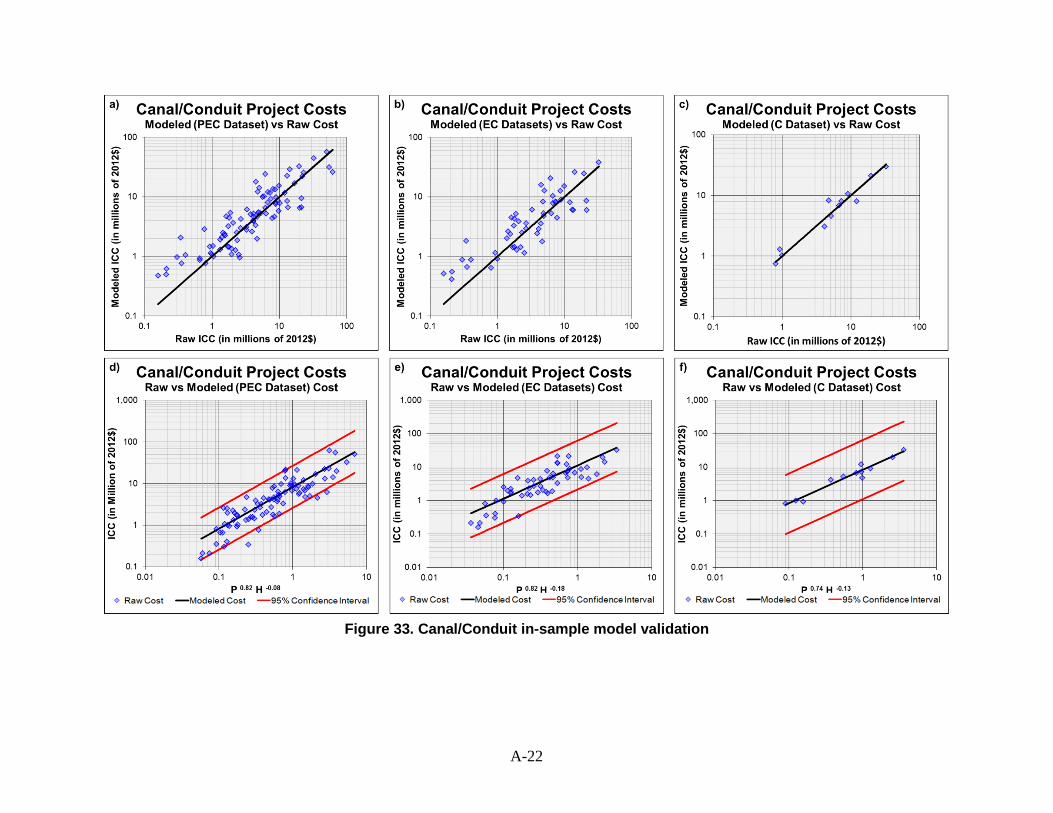
A-22
Figure 33. Canal/Conduit in-sample model validation
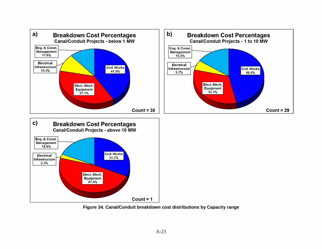
A-23
Figure 34. Canal/Conduit breakdown cost distributions by Capacity range

A-24
Figure 35. Canal/Conduit breakdown cost distributions by Head range
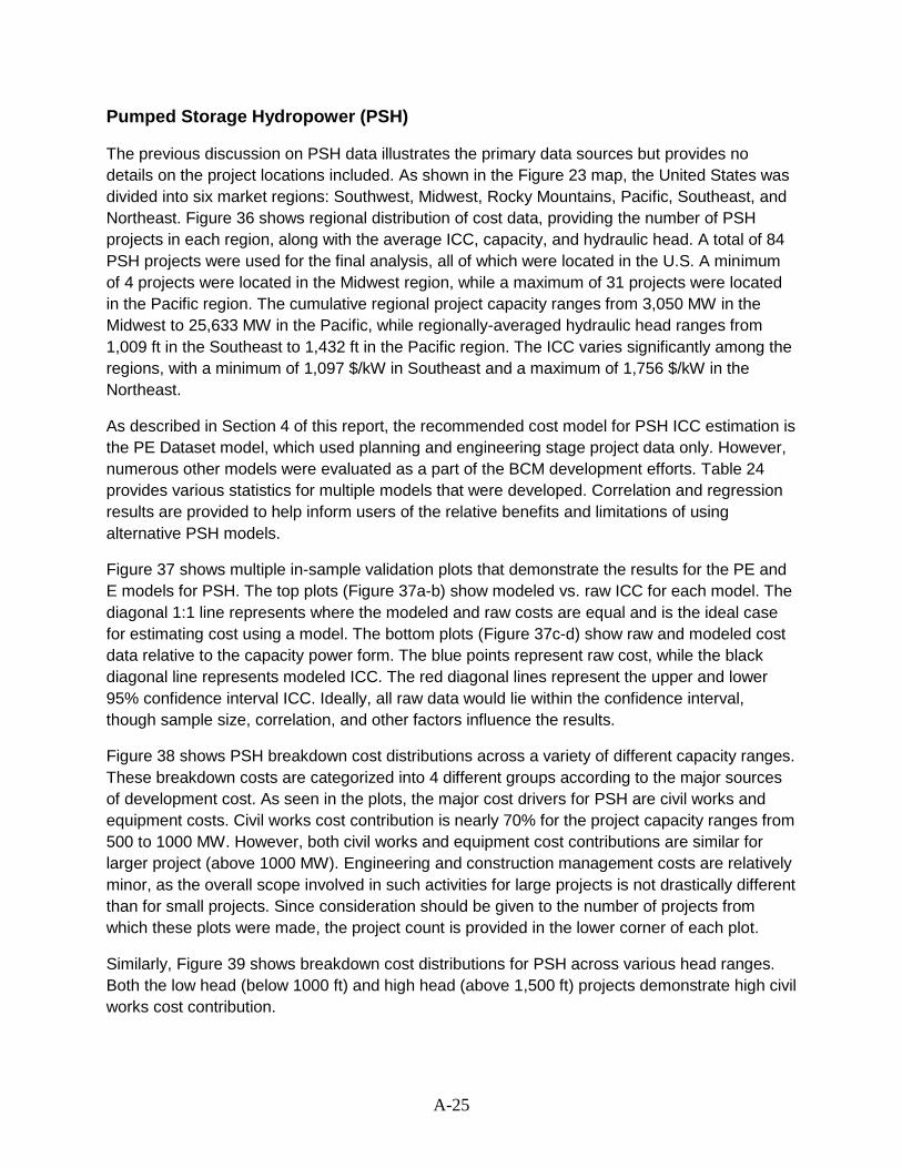
A-25
Pumped Storage Hydropower (PSH)
The previous discussion on PSH data illustrates the primary data sources but provides no
details on the project locations included. As shown in the Figure 23 map, the United States was
divided into six market regions: Southwest, Midwest, Rocky Mountains, Pacific, Southeast, and
Northeast. Figure 36 shows regional distribution of cost data, providing the number of PSH
projects in each region, along with the average ICC, capacity, and hydraulic head. A total of 84
PSH projects were used for the final analysis, all of which were located in the U.S. A minimum
of 4 projects were located in the Midwest region, while a maximum of 31 projects were located
in the Pacific region. The cumulative regional project capacity ranges from 3,050 MW in the
Midwest to 25,633 MW in the Pacific, while regionally-averaged hydraulic head ranges from
1,009 ft in the Southeast to 1,432 ft in the Pacific region. The ICC varies significantly among the
regions, with a minimum of 1,097 $/kW in Southeast and a maximum of 1,756 $/kW in the
Northeast.
As described in Section 4 of this report, the recommended cost model for PSH ICC estimation is
the PE Dataset model, which used planning and engineering stage project data only. However,
numerous other models were evaluated as a part of the BCM development efforts. Table 24
provides various statistics for multiple models that were developed. Correlation and regression
results are provided to help inform users of the relative benefits and limitations of using
alternative PSH models.
Figure 37 shows multiple in-sample validation plots that demonstrate the results for the PE and
E models for PSH. The top plots (Figure 37a-b) show modeled vs. raw ICC for each model. The
diagonal 1:1 line represents where the modeled and raw costs are equal and is the ideal case
for estimating cost using a model. The bottom plots (Figure 37c-d) show raw and modeled cost
data relative to the capacity power form. The blue points represent raw cost, while the black
diagonal line represents modeled ICC. The red diagonal lines represent the upper and lower
95% confidence interval ICC. Ideally, all raw data would lie within the confidence interval,
though sample size, correlation, and other factors influence the results.
Figure 38 shows PSH breakdown cost distributions across a variety of different capacity ranges.
These breakdown costs are categorized into 4 different groups according to the major sources
of development cost. As seen in the plots, the major cost drivers for PSH are civil works and
equipment costs. Civil works cost contribution is nearly 70% for the project capacity ranges from
500 to 1000 MW. However, both civil works and equipment cost contributions are similar for
larger project (above 1000 MW). Engineering and construction management costs are relatively
minor, as the overall scope involved in such activities for large projects is not drastically different
than for small projects. Since consideration should be given to the number of projects from
which these plots were made, the project count is provided in the lower corner of each plot.
Similarly, Figure 39 shows breakdown cost distributions for PSH across various head ranges.
Both the low head (below 1000 ft) and high head (above 1,500 ft) projects demonstrate high civil
works cost contribution.
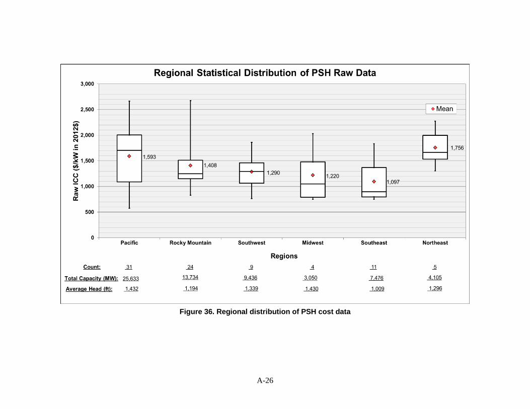
A-26
Figure 36. Regional distribution of PSH cost data
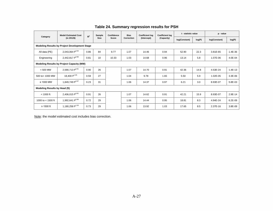
A-27
Table 24. Summary regression results for PSH
Category Model Estimated Cost
(in 2012$) R2
Sample
Size
Confidence
Score
Bias
Correction
Coefficient log
(Intercept)
Coefficient log
(Capacity)
t - statistic value p - value
log(Constant) log(P) log(Constant) log(P)
Modeling Results by Project Development Stage
All data (PE) 2,043,064 P0.94
0.86 84 9.77 1.07 14.46 0.94 52.90 22.3 3.81E-65 1.4E-36
Engineering 2,442,817 P0.96
0.81 10 10.33 1.03 14.68 0.96 13.14 5.8 1.07E-06 4.0E-04
Modeling Results by Project Capacity (MW)
< 500 MW 2,590,713 P0.91
0.90 26 1.07 14.70 0.91 42.36 14.8 4.53E-24 1.4E-13
500 to< 1000 MW 18,400 P1.65
0.59 27 1.04 9.78 1.65 5.50 5.9 1.02E-05 3.3E-06
≥ 1000 MW 1,849,749 P0.97
0.23 31 1.06 14.37 0.97 6.21 3.0 8.93E-07 5.8E-03
Modeling Results by Head (ft)
< 1000 ft 2,406,015 P0.91
0.91 26 1.07 14.62 0.91 42.21 15.9 8.93E-07 2.9E-14
1000 to < 1500 ft 1,992,641 P0.95
0.72 29 1.06 14.44 0.95 18.81 8.3 4.94E-24 6.2E-09
≥ 1500 ft 1,180,258 P1.03
0.73 29 1.06 13.92 1.03 17.65 8.5 2.37E-16 3.8E-09
Note: the model estimated cost includes bias correction.
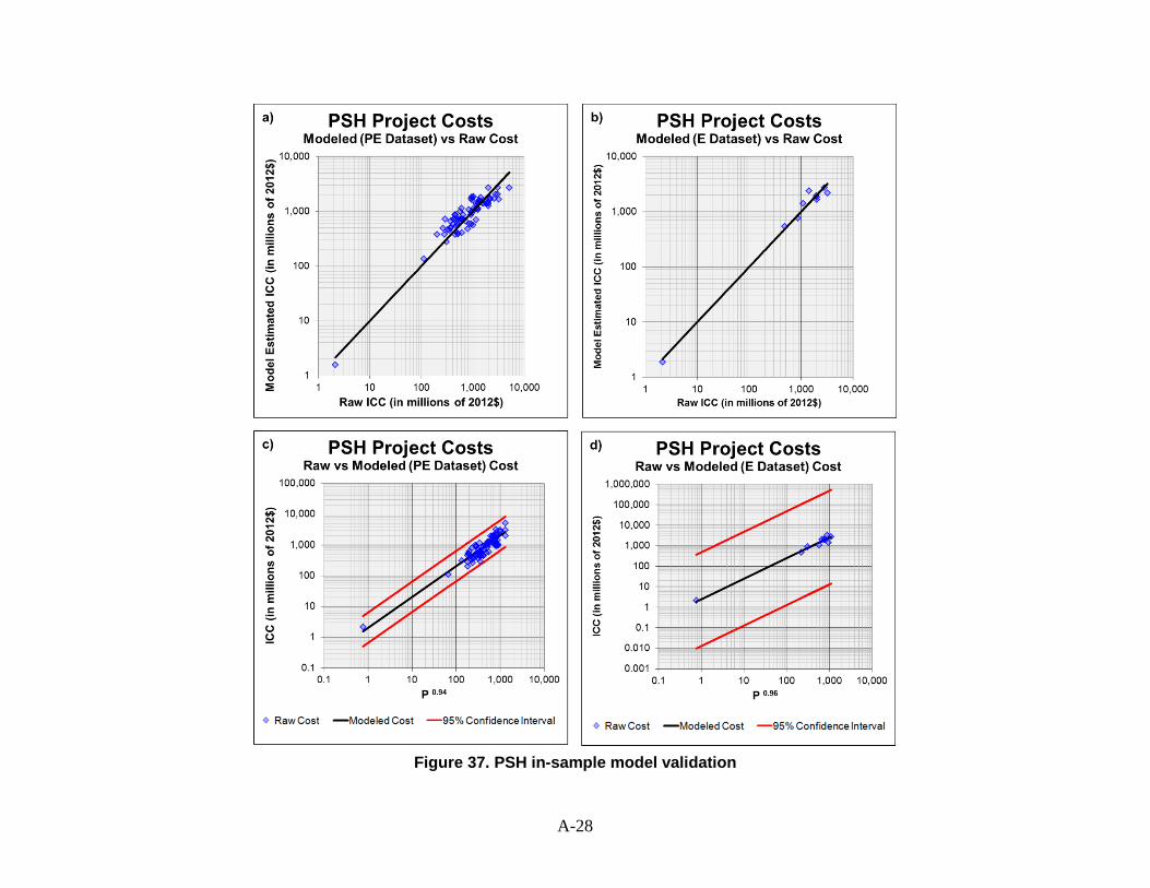
A-28
Figure 37. PSH in-sample model validation
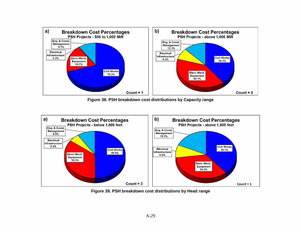
A-29
Figure 38. PSH breakdown cost distributions by Capacity range
Figure 39. PSH breakdown cost distributions by Head range

A-30
Unit Addition and Generator Rewind
The previous discussion on Unit Addition and Generator Rewind data illustrates the primary
data sources but provides no details on the project locations included. As shown in the Figure
23 map, the United States was divided into six market regions: Southwest, Midwest, Rocky
Mountains, Pacific, Southeast, and Northeast. Figure 40 and Figure 41 show regional
distribution of cost data, providing the number of projects in each region, along with the average
ICC and total capacity for Unit Addition and Generator Rewind respectively. No Unit Addition
project data were available for the Southeast region. Also, no Generator Rewind data were
available for the Midwest region. A total of 13 Unit Addition and 21 Generator Rewind projects
were used for the final analysis.
Table 25 provides a summary of various statistics for each model that was developed for Unit
Addition and Generator Rewind in Section 4. As the raw data were limited to a relatively small
sample size, only the PEC Model was developed. Figure 42 shows in-sample validation plots
that illustrate the model results. The modeled vs. raw ICC with the diagonal 1:1 line represents
the points at which the modeled and raw costs are equal. Figure 43 shows raw and modeled
cost data relative to the capacity power form. The blue points represent raw cost, while the
black diagonal line represents modeled ICC. The red diagonal lines represent the upper and
lower 95% confidence interval ICC. Ideally, all raw data would lie within the confidence interval,
though sample size, correlation, and other factors influence the results.
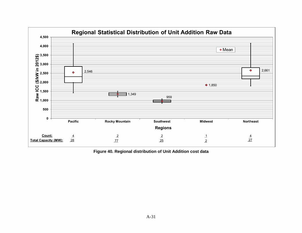
A-31
Figure 40. Regional distribution of Unit Addition cost data

A-32
Figure 41. Regional distribution of Generator Rewind cost data
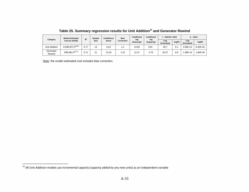
A-33
Table 25. Summary regression results for Unit Addition16 and Generator Rewind
Category Model Estimated
Cost (in 2012$) R2
Sample
Size Confidence
Score Bias
Correction
Coefficient
log
(Intercept)
Coefficient
log
(Capacity)
t - statistic value p - value
Log
(Constant) log(P)
Log
(Constant) log(P)
Unit Addition 3,030,671 P0.81 0.77 13 9.24 1.1 14.83 0.81 49.7 6.1 2.69E-14 8.20E-05
Generator
Rewind 299,461 P0.75 0.71 21 10.29 1.15 12.47 0.75 26.37 6.8 1.98E-16 1.80E-06
Note: the model estimated cost includes bias correction.
16
All Unit Addition models use incremental capacity (capacity added by any new units) as an independent variable

B-34
Figure 42. Unit Addition and Generator Rewind in-sample model validation
Figure 43. Unit Addition and Generator Rewind in-sample model validation
Recommended