1
Homogeneous Coordinates
Jules Bloomenthal and Jon Rokne
Department of Computer Science
The University of Calgary
Introduction
Homogeneous coordinates have a natural application to Computer Graphics; they form a basis for
the projective geometry used extensively to project a three-dimensional scene onto a two-
dimensional image plane. They also unify the treatment of common graphical transformations and
operations. The graphical use of homogeneous coordinates is due to [Roberts, 1965], and an early
review is presented by [Ahuja, 1968]. Today, homogeneous coordinates are presented in numerous
computer graphics texts (such as [Foley, Newman, Rogers, Qiulin and Davies]); [Newman], in
particular, provides an appendix of homogeneous techniques. [Riesenfeld] provides an excellent
introduction to homogeneous coordinates and their algebraic, geometric and topological
significance to Computer Graphics. [Bez] further discusses their algebraic and topological
properties, and [Blinn77, Blinn78] develop additional applications for Computer Graphics.
Homogeneous coordinates are also used in the related areas of CAD/CAM [Zeid], robotics
[McKerrow], surface modeling [Farin], and computational projective geometry [Kanatani]. They
can also extend the number range for fixed point arithmetic [Rogers].
Our aim here is to provide an intuitive yet theoretically based discussion that assembles the key
features of homogeneous coordinates and their applications to Computer Graphics. These
applications include affine transformations, perspective projection, line intersections, clipping, and
rational curves and surfaces. For the sake of clarity in accompanying illustrations, we confine our
2
development to two dimensions and then use the intuition gained to present the application of
homogeneous coordinates to three dimensions. None of the material presented here is new; rather,
we have tried to collect in one place diverse but related methods.
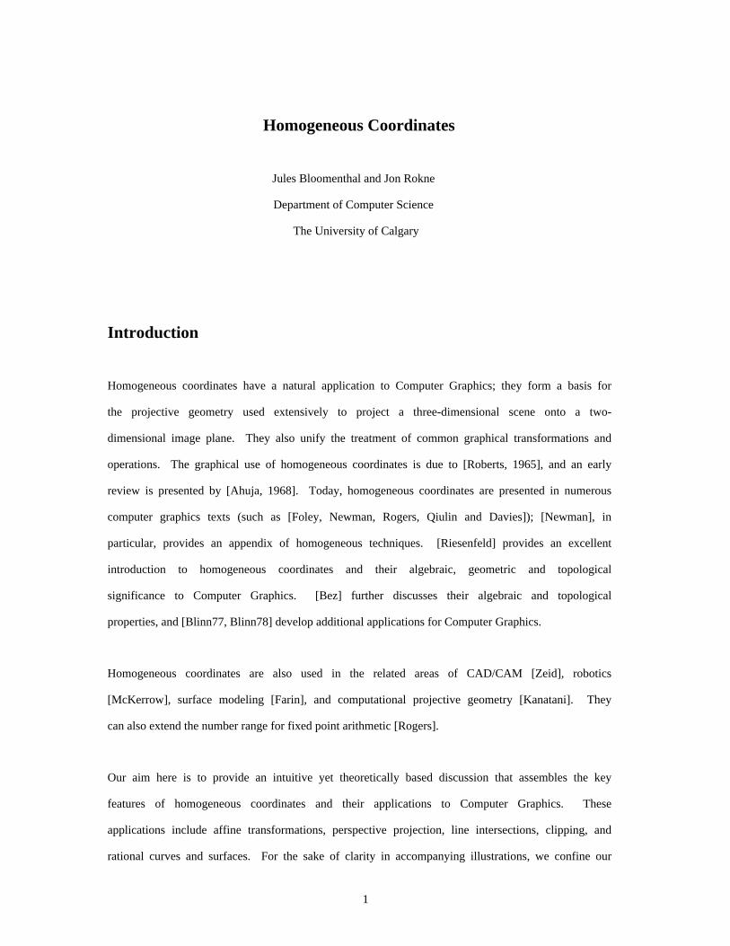
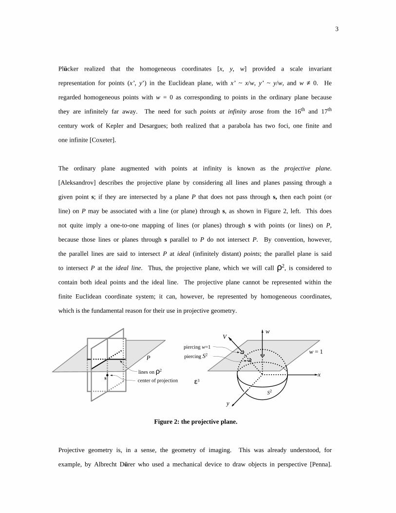
[Kline] provides a brief history of homogeneous coordinates, crediting Möbius with their
introduction [Möbius]. Given a fixed triangle in the plane, Möbius defined a set of homogeneous
coordinates for a point p to be the weights required at the triangle vertices such that p became the
center of gravity of the triangle (Figure 1, left). The point p is computed as (waa, wbb, wcc), with
the condition that wa+wb+wc = 1. The three unknowns wa, wb, and wc, are called the barycentric
coordinates of p with respect to a, b, and c. [Snyder] provides an algorithm for computing wi;
[Farin] relates w to area by wa = Aa/(Aa+Ab+Ac) and similarly for wb and wc (Figure 1, middle).
Plücker defined another set of homogeneous coordinates by considering the signed distances from
a point to the edges of a fixed triangle (Figure 1, right); here, p = (la, lb, lc).
wa
wb
wc
AaAc
Ab
a
b
c
lalb
lca
b
c
a
b
c
balancepoint p
Figure 1: barycentric and Plücker coordinates.
Barycentric and Plücker coordinates are examples of coordinate systems in which n+1 values
represent an n-dimensional point. One immediate attribute of these systems is the invariance of a
point when scaled: scaling the Möbius weights or the size of the Plücker triangle does not change
the position of p. As an aside, we note that higher dimensional Plücker coordinates have been
applied to ray-tracing [Pellegrini] (for an exposition of n-dimensional Plücker coordinates, also
known as Grassmann coordinates, see [Stolfi]).
Homogeneous Coordinates for the Projective Plane
3
Plücker realized that the homogeneous coordinates [x, y, w] provided a scale invariant
representation for points (x’, y’) in the Euclidean plane, with x’ ~ x/w, y’ ~ y/w, and w ≠ 0. He
regarded homogeneous points with w = 0 as corresponding to points in the ordinary plane because
they are infinitely far away. The need for such points at infinity arose from the 16th and 17th
century work of Kepler and Desargues; both realized that a parabola has two foci, one finite and
one infinite [Coxeter].
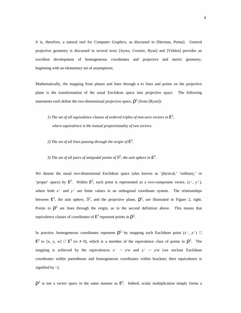
The ordinary plane augmented with points at infinity is known as the projective plane.
[Aleksandrov] describes the projective plane by considering all lines and planes passing through a
given point s; if they are intersected by a plane P that does not pass through s, then each point (or
line) on P may be associated with a line (or plane) through s, as shown in Figure 2, left. This does
not quite imply a one-to-one mapping of lines (or planes) through s with points (or lines) on P,
because those lines or planes through s parallel to P do not intersect P. By convention, however,
the parallel lines are said to intersect P at ideal (infinitely distant) points; the parallel plane is said
to intersect P at the ideal line. Thus, the projective plane, which we will call ρ2, is considered to
contain both ideal points and the ideal line. The projective plane cannot be represented within the
finite Euclidean coordinate system; it can, however, be represented by homogeneous coordinates,
which is the fundamental reason for their use in projective geometry.
piercing w=1
piercing S2
S2
w = 1
Vw
y
x
P
ε3slines on ρ2
center of projection
Figure 2: the projective plane.
Projective geometry is, in a sense, the geometry of imaging. This was already understood, for
example, by Albrecht Dürer who used a mechanical device to draw objects in perspective [Penna].
4
It is, therefore, a natural tool for Computer Graphics, as discussed in [Herman, Penna]. General
projective geometry is discussed in several texts [Ayres, Coxeter, Ryan] and [Veblen] provides an
excellent development of homogeneous coordinates and projective and metric geometry,
beginning with an elementary set of assumptions.
Mathematically, the mapping from planes and lines through s to lines and points on the projective
plane is the transformation of the usual Euclidean space into projective space. The following
statements each define the two-dimensional projective space, ρ2 (from [Ryan]):
1) The set of all equivalence classes of ordered triples of non-zero vectors in ε3,
where equivalence is the mutual proportionality of two vectors.
2) The set of all lines passing through the origin of ε3.
3) The set of all pairs of antipodal points of S2, the unit sphere in ε3.
We denote the usual two-dimensional Euclidean space (also known as ‘physical,’ ‘ordinary,’ or
‘proper’ space) by ε2. Within ε2, each point is represented as a two-component vector, (x’, y’),
where both x’ and y’ are finite values in an orthogonal coordinate system. The relationships
between ε3, the unit sphere, S2, and the projective plane, ρ2, are illustrated in Figure 2, right.
Points in ρ2 are lines through the origin, as in the second definition above. This means that
equivalence classes of coordinates of ε3 represent points in ρ2.
In practice, homogeneous coordinates represent ρ2 by mapping each Euclidean point (x’, y’) ∈
ε2 to [x, y, w] ∈ ε3 (w ≠ 0), which is a member of the equivalence class of points in ρ2. The
mapping is achieved by the equivalences x’ ~ x/w and y’ ~ y/w (we enclose Euclidean
coordinates within parentheses and homogeneous coordinates within brackets; their equivalence is
signified by ~).
ρ2 is not a vector space in the same manner as ε2. Indeed, scalar multiplication simply forms a
5
new representative of the equivalence class. Furthermore, if the representatives are chosen from
the intersection with the plane w = 1, then the vector addition of two points in ρ2 computes a
representative of the midpoint between the two vectors (for example, given two ordinary vectors,
(1, 2) and (3, 4), addition of their homogeneous equivalents is [1, 2, 1]+[3, 4, 1] = [4, 6, 2] ~ (2, 3)).
The division by w means that the conversion of a homogeneous point to its Euclidean equivalent is
inherently a projection of the homogenous point onto the w = 1 plane. Figure 2, right, illustrates
this projection in the two-dimensional case; three-dimensional homogeneous points on the S2
sphere are projected onto the w = 1 plane. [Riesenfeld] provides an illustration of four-
dimensional homogeneous points projected onto a three-dimensional hyper-plane.
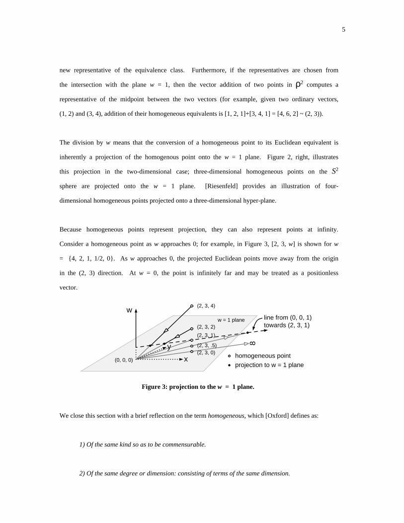
Because homogeneous points represent projection, they can also represent points at infinity.
Consider a homogeneous point as w approaches 0; for example, in Figure 3, [2, 3, w] is shown for w
= {4, 2, 1, 1/2, 0}. As w approaches 0, the projected Euclidean points move away from the origin
in the (2, 3) direction. At w = 0, the point is infinitely far and may be treated as a positionless
vector.
(2, 3, 0)
(2, 3, 1)
(2, 3, 2)
(2, 3, 4)
x
y 8
ww = 1 plane
projection to w = 1 plane
homogeneous point
line from (0, 0, 1) towards (2, 3, 1)
(0, 0, 0)
(2, 3, .5)
Figure 3: projection to the w = 1 plane.
We close this section with a brief reflection on the term homogeneous, which [Oxford] defines as:
1) Of the same kind so as to be commensurable.
2) Of the same degree or dimension: consisting of terms of the same dimension.
6
With this in mind, consider a general conic in ε2:
f(x’, y’) = ax’2 +by’2 +cx’y’ +dx’ +ey’ + f = 0.
The homogeneous form for the conic is found by replacing x’ with x/w and y’ with y/w;
multiplying by w2 yields:
f*(x, y, w) = ax2+by2 +cxy +dxw +eyw +fw2 = 0.
Here, all terms have total variable degree two, as in definition 2), above. In passing, we note that
any polynomial function in ε2 has a form equivalent to f and may be transformed, via a change to
homogeneous coordinates, to a polynomial function with constant total degree for each term. This
holds for any polynomial function in a finitely dimensioned space.
Homogeneous Coordinates for Two Dimensions
An important, practical aspect of the homogeneous coordinate system is its unification of the
translation, scaling and rotation of geometric objects. In ε2 Euclidean space, the most general
affine mapping is
p’ = pA+c, or (px’, py’) = (px, py)A+(cx, cy),
where p’ and p are points in ε2, A is a 2 by 2 matrix representing scaling and rotation, and the
point c represents translation. In this formulation, translation is treated differently from rotation
or scaling.
If, however, p is represented as a homogeneous point [px py 1] and a 2 × 3 matrix is employed,
7
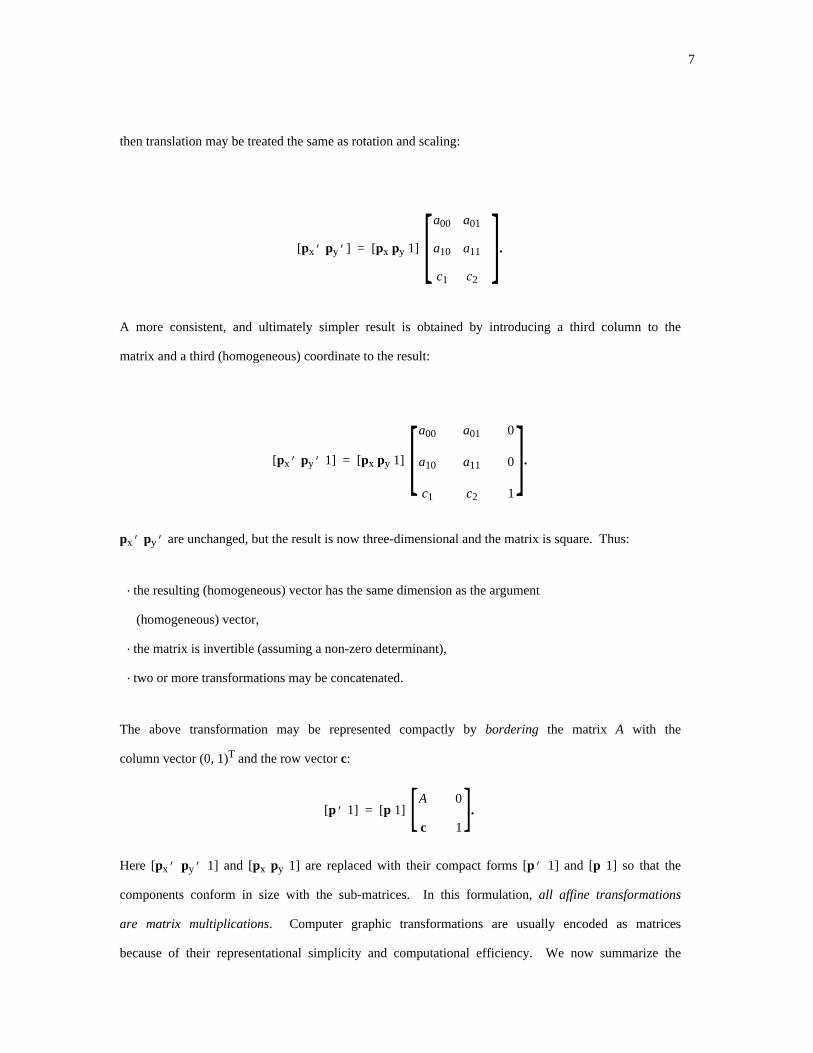
then translation may be treated the same as rotation and scaling:
[px’ py’] = [px py 1] [c2c1
a11a10
a01a00 ].
A more consistent, and ultimately simpler result is obtained by introducing a third column to the
matrix and a third (homogeneous) coordinate to the result:
[px’ py’ 1] = [px py 1] [1c2c1
0a11a10
0a01a00 ].
px’ py’ are unchanged, but the result is now three-dimensional and the matrix is square. Thus:
· the resulting (homogeneous) vector has the same dimension as the argument
(homogeneous) vector,
· the matrix is invertible (assuming a non-zero determinant),
· two or more transformations may be concatenated.
The above transformation may be represented compactly by bordering the matrix A with the
column vector (0, 1)T and the row vector c:
[p’ 1] = [p 1] [ 1c
0A ].Here [px’ py’ 1] and [px py 1] are replaced with their compact forms [p’ 1] and [p 1] so that the
components conform in size with the sub-matrices. In this formulation, all affine transformations
are matrix multiplications. Computer graphic transformations are usually encoded as matrices
because of their representational simplicity and computational efficiency. We now summarize the
8
use of homogeneous coordinates for affine transformations.
Affine Transformations
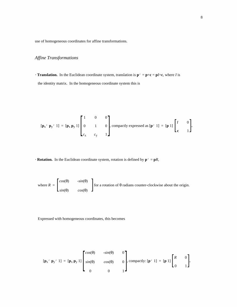
· Translation. In the Euclidean coordinate system, translation is p’ = p+c = pI+c, where I is
the identity matrix. In the homogeneous coordinate system this is
[px’ py’ 1] = [px py 1] [1cycx
010
001
], compactly expressed as [p’ 1] = [p 1] [ 1c
0I ].
· Rotation. In the Euclidean coordinate system, rotation is defined by p’ = pR,
where R = [ cos(θ) sin(θ)
-sin(θ) cos(θ) ] for a rotation of θ radians counter-clockwise about the origin.
Expressed with homogeneous coordinates, this becomes
[px’ py’ 1] = [px py 1] [100
0cos(θ)sin(θ)
0-sin(θ)cos(θ)
], compactly: [p’ 1] = [p 1] [ 10
0R ].
9
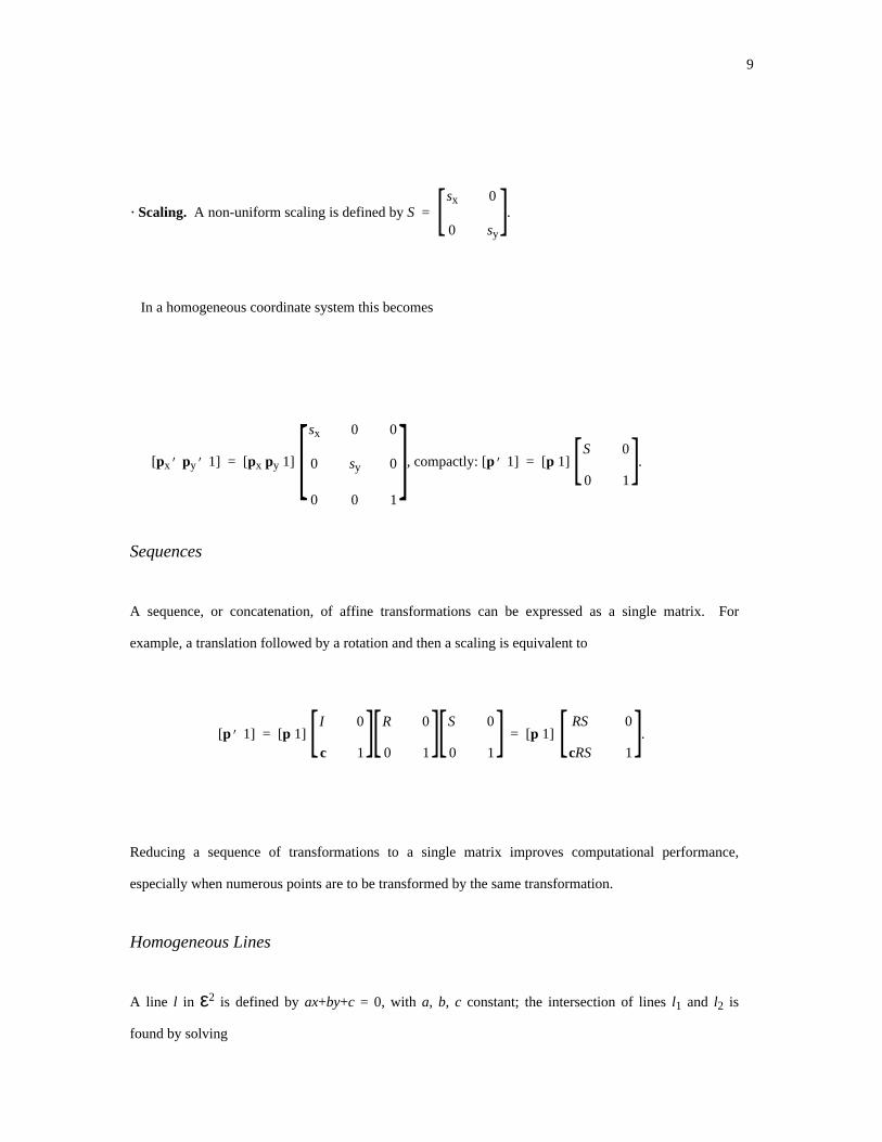
· Scaling. A non-uniform scaling is defined by S = [ sy0
0sx ].
In a homogeneous coordinate system this becomes
[px’ py’ 1] = [px py 1] [100
0sy0
00sx ], compactly: [p’ 1] = [p 1] [ 10
0S ].
Sequences
A sequence, or concatenation, of affine transformations can be expressed as a single matrix. For
example, a translation followed by a rotation and then a scaling is equivalent to
[p’ 1] = [p 1] [ 1c
0I ][ 10
0R ][ 10
0S ] = [p 1] [ 1cRS
0RS ].
Reducing a sequence of transformations to a single matrix improves computational performance,
especially when numerous points are to be transformed by the same transformation.
Homogeneous Lines
A line l in ε2 is defined by ax+by+c = 0, with a, b, c constant; the intersection of lines l1 and l2 is
found by solving
10
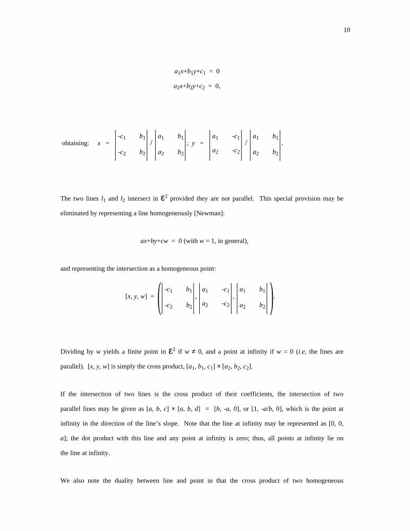
a1x+b1y+c1 = 0
a2x+b2y+c2 = 0,
obtaining: x = | b2-c2
b1-c1 | / | b2a2
b1a1 |; y = | -c2a2
-c1a1 | / | b2a2
b1a1 |.
The two lines l1 and l2 intersect in ε2 provided they are not parallel. This special provision may be
eliminated by representing a line homogeneously [Newman]:
ax+by+cw = 0 (with w = 1, in general),
and representing the intersection as a homogeneous point:
[x, y, w] = (| b2-c2
b1-c1 |, | -c2a2
-c1a1 |, | b2a2
b1a1 | ).
Dividing by w yields a finite point in ε2 if w ≠ 0, and a point at infinity if w = 0 (i.e, the lines are
parallel). [x, y, w] is simply the cross product, [a1, b1, c1] × [a2, b2, c2].
If the intersection of two lines is the cross product of their coefficients, the intersection of two
parallel lines may be given as [a, b, c] × [a, b, d] = [b, -a, 0], or [1, -a/b, 0], which is the point at
infinity in the direction of the line’s slope. Note that the line at infinity may be represented as [0, 0,
a]; the dot product with this line and any point at infinity is zero; thus, all points at infinity lie on
the line at infinity.
We also note the duality between line and point in that the cross product of two homogeneous

11
points yields the coordinates of their connecting line. This duality between point and line in two
dimensions has, in three dimensions, a corresponding duality between point and plane. See
[Blinn77] for the use of homogeneous coordinates to represent lines in ε3.
Conics
In our introduction we briefly touched upon the general second degree implicit curve in ε2,
showing that it could be converted to homogeneous form in ρ2 (represented by points in ε3). This
curve is either null, a conic section, a single point, intersecting lines, or coincident lines [Blinn84,
Brieskorn].
It can also be shown that conic sections are equivalent under perspective transformation. As an
example, consider the transformation of a circle to an ellipse, both conic sections. Let such a cone
be defined and let a plane A intersect the cone to form an ellipse. Now intersect the cone with a
plane B normal to the cone axis at a distance from the cone vertex such that the circle of
intersection has the desired radius. The ellipse in plane A is simply the projection of the circle in
plane B, with the axis of the cone being the direction of projection.
BA
Figure 4: conic section as a projection.
We can define second degree curves as the set of all points [x, y, w] that satisfy the general
homogeneous equation of degree 2:
ax2+by2+cxy+dxw+eyw+fw2 = 0, which can be written in matrix form as:
12
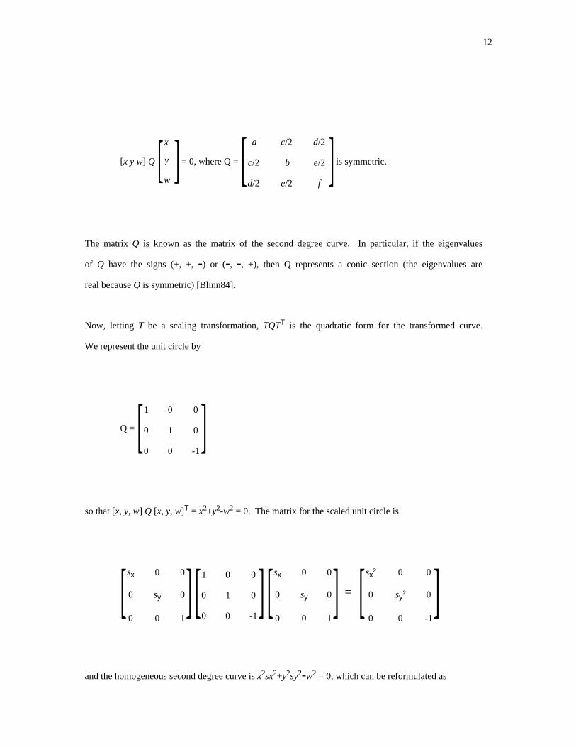
[x y w] Q [w
y
x
] = 0, where Q = [fe/2d/2
e/2bc/2
d/2c/2a
] is symmetric.
The matrix Q is known as the matrix of the second degree curve. In particular, if the eigenvalues
of Q have the signs (+, +, -) or (-, -, +), then Q represents a conic section (the eigenvalues are
real because Q is symmetric) [Blinn84].
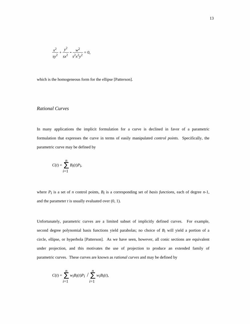
Now, letting T be a scaling transformation, TQTT is the quadratic form for the transformed curve.
We represent the unit circle by
Q = [-100
010
001 ]so that [x, y, w] Q [x, y, w]T = x2+y2-w2 = 0. The matrix for the scaled unit circle is
[100
0sy0
00sx ] [-100
010
001 ] [100
0sy0
00sx ] = [-100
0sy20
00sx2
]and the homogeneous second degree curve is x2sx2+y2sy2-w2 = 0, which can be reformulated as
13
x2
sy2 +
y2
sx2 -
w2
s2x2y2 = 0,
which is the homogeneous form for the ellipse [Patterson].
Rational Curves
In many applications the implicit formulation for a curve is declined in favor of a parametric
formulation that expresses the curve in terms of easily manipulated control points. Specifically, the
parametric curve may be defined by
C(t) = n
Σi=1
Bi(t)Pi,
where Pi is a set of n control points, Bi is a corresponding set of basis functions, each of degree n-1,
and the parameter t is usually evaluated over (0, 1).
Unfortunately, parametric curves are a limited subset of implicitly defined curves. For example,
second degree polynomial basis functions yield parabolas; no choice of Bi will yield a portion of a
circle, ellipse, or hyperbola [Patterson]. As we have seen, however, all conic sections are equivalent
under projection, and this motivates the use of projection to produce an extended family of
parametric curves. These curves are known as rational curves and may be defined by
C(t) = n
Σi=1
wiBi(t)Pi / n
Σi=1
wiBi(t),
14
where wi are weights applied to the control vertices. Increasing the value of a weight draws the
curve closer to the corresponding control point. Usually wi > 0 (otherwise the resulting curve may
be undefined or contain asymptotes [Patterson]) and usually the basis functions form a partition of
unity, meaning ΣBi(t) = 1, which implies that the shape of the curve is unaffected by translation
of the control points [Barsky].
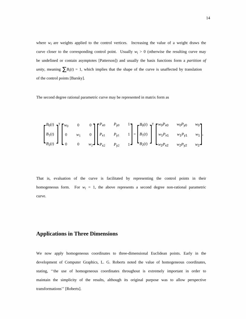
The second degree rational parametric curve may be represented in matrix form as
[B2(t)
B1(t)
B0(t)
]T
[w200
0w10
00w0 ] [1Py2Px2
1Py1Px1
1Py0Px0
] = [B2(t)
B1(t)
B0(t)
]T
[w2w2Py2w2Px2
w1w1Py1w1Px1
w0w0Py0w0Px0
].
That is, evaluation of the curve is facilitated by representing the control points in their
homogeneous form. For wi = 1, the above represents a second degree non-rational parametric
curve.
Applications in Three Dimensions
We now apply homogeneous coordinates to three-dimensional Euclidean points. Early in the
development of Computer Graphics, L. G. Roberts noted the value of homogeneous coordinates,
stating, ‘‘the use of homogeneous coordinates throughout is extremely important in order to
maintain the simplicity of the results, although its original purpose was to allow perspective
transformations’’ [Roberts].
15
In other words, the use of the additional, homogeneous coordinate not only produces polynomials
of fixed degree, it also provides a method for consistent manipulation of the Euclidean space.
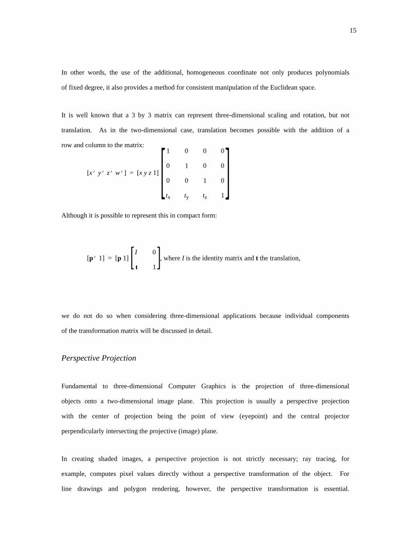
It is well known that a 3 by 3 matrix can represent three-dimensional scaling and rotation, but not
translation. As in the two-dimensional case, translation becomes possible with the addition of a
row and column to the matrix:
[x’ y’ z’ w’] = [x y z 1] [1tztytx
0100
0010
0001
]Although it is possible to represent this in compact form:
[p’ 1] = [p 1] [ 1t
0I ], where I is the identity matrix and t the translation,
we do not do so when considering three-dimensional applications because individual components
of the transformation matrix will be discussed in detail.
Perspective Projection
Fundamental to three-dimensional Computer Graphics is the projection of three-dimensional
objects onto a two-dimensional image plane. This projection is usually a perspective projection
with the center of projection being the point of view (eyepoint) and the central projector
perpendicularly intersecting the projective (image) plane.
In creating shaded images, a perspective projection is not strictly necessary; ray tracing, for
example, computes pixel values directly without a perspective transformation of the object. For
line drawings and polygon rendering, however, the perspective transformation is essential.
16
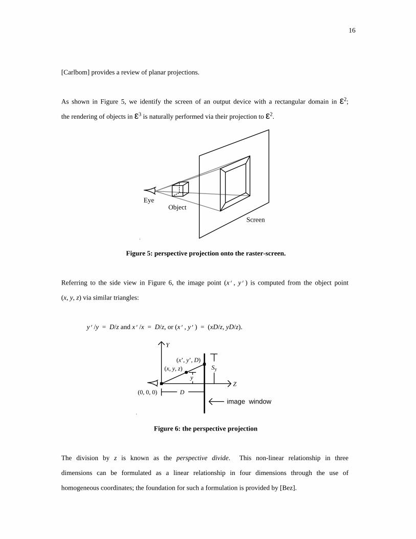
[Carlbom] provides a review of planar projections.
As shown in Figure 5, we identify the screen of an output device with a rectangular domain in ε2;
the rendering of objects in ε3 is naturally performed via their projection to ε2.
Screen
ObjectEye
Figure 5: perspective projection onto the raster-screen.
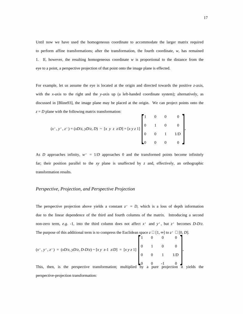
Referring to the side view in Figure 6, the image point (x’, y’) is computed from the object point
(x, y, z) via similar triangles:
y’/y = D/z and x’/x = D/z, or (x’, y’) = (xD/z, yD/z).
image window
(x, y, z)
(0, 0, 0) DZ
Y
Sy
(x’, y’, D)
y
Figure 6: the perspective projection
The division by z is known as the perspective divide. This non-linear relationship in three
dimensions can be formulated as a linear relationship in four dimensions through the use of
homogeneous coordinates; the foundation for such a formulation is provided by [Bez].
17
Until now we have used the homogeneous coordinate to accommodate the larger matrix required
to perform affine transformations; after the transformation, the fourth coordinate, w, has remained
1. If, however, the resulting homogeneous coordinate w is proportional to the distance from the
eye to a point, a perspective projection of that point onto the image plane is effected.
For example, let us assume the eye is located at the origin and directed towards the positive z-axis,
with the x-axis to the right and the y-axis up (a left-handed coordinate system); alternatively, as
discussed in [Blinn93], the image plane may be placed at the origin. We can project points onto the
z = D plane with the following matrix transformation:
(x’, y’, z’) = (xD/z, yD/z, D) ~ [x y z z/D] = [x y z 1] [0000
1/D100
0010
0001
].
As D approaches infinity, w’ = 1/D approaches 0 and the transformed points become infinitely
far; their position parallel to the xy plane is unaffected by z and, effectively, an orthographic
transformation results.
Perspective, Projection, and Perspective Projection
The perspective projection above yields a constant z’ = D, which is a loss of depth information
due to the linear dependence of the third and fourth columns of the matrix. Introducing a second
non-zero term, e.g. -1, into the third column does not affect x’ and y’, but z’ becomes D-D/z.
The purpose of this additional term is to compress the Euclidean space z ∈ [1, ∞] to z’ ∈ [0, D].
(x’, y’, z’) = (xD/z, yD/z, D-D/z) ~ [x y z-1 z/D] = [x y z 1] [0-100
1/D100
0010
0001
].
This, then, is the perspective transformation; multiplied by a pure projection it yields the
perspective-projection transformation:
18
[0-100
1/D100
0010
0001
][1D00
0000
0010
0001
] = [0000
1/D100
0010
0001
].
perspective projection perspective-projection
Perspective Space
The homogeneous perspective transformation transforms Euclidean points in ε3 (represented as
homogeneous points) to new homogeneous points, which may then be converted to Euclidean
space. These transformed points exist in perspective space. We now examine the properties of the
perspective transformation in terms of the relation between perspective space and the
untransformed object space.
In an affine transformation matrix, the last column is [0 0 0 1]T; multiplication with a direction
vector [a, b, c, 0] yields another direction vector [a’, b’, c’, 0]. In a perspective transform,
however, the last column is [0 0 -1/D 1]T; multiplication with a direction vector yields [a’, b’, c’,
-c/D]. This is a homogeneous point, not direction, and is known as the vanishing point for the
given direction. A set of three-dimensional parallel lines will intersect at the same vanishing point,
with the one exception that parallel lines in the xy plane remain parallel.
In many graphics systems, points in object space are transformed by a matrix that is the
concatenation of all rotation, scaling, translation, and perspective transformations. Usually the
projection transformation is not incorporated into this concatenation, for several reasons. First, the
perspective matrix is invertible whereas the perspective-projection matrix is singular. Secondly,
the value of z’ before projection is often useful for incremental scanline depth sorting or for
intensity variation in line drawings. More importantly, however, z’ can simplify three-
dimensional clipping of Euclidean lines and line segments against the viewing frustum by clipping
homogeneously against a parallelepiped. After clipping, points are simply projected to the z = D
image plane and displayed.
19
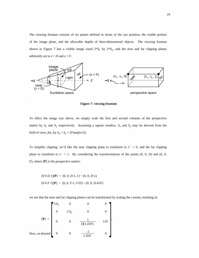
The viewing frustum consists of six planes defined in terms of the eye position, the visible portion
of the image plane, and the allowable depths of three-dimensional objects. The viewing frustum
shown in Figure 7 has a visible image sized 2*Sx by 2*Sy, and the near and far clipping planes
arbitrarily set to z = D and z = F.
top
farright
Sy
ZSy
near
imageplane
(z = D)
(z = F) ( SySx, , 0) ( SySx, , 1)ne
ar far
8
Euclidean space perspective space
Figure 7: viewing frustum
To effect the image size above, we simply scale the first and second columns of the perspective
matrix by Sx and Sy respectively. Assuming a square window, Sx and Sy may be derived from the
field of view, fov, by Sx = Sy = D.tan(fov/2).
To simplify clipping, we’d like the near clipping plane to transform to z’ = 0, and the far clipping
plane to transform to z’ = 1. By considering the transformations of the points (0, 0, D) and (0, 0,
F), where [P] is the perspective matrix:
[0 0 D 1][P] = [0, 0, D-1, 1] ~ (0, 0, D-1)
[0 0 F 1][P] = [0, 0, F-1, F/D] ~ (0, 0, D-D/F)
we see that the near and far clipping planes can be transformed by scaling the z-terms, resulting in:
[P] = [0-1
1-D/F00
1/D1D(1-D/F)
00
001/Sy0
0001/Sx
].
Now, as desired:
20
[0 0 D 1][P] = [0, 0, DD(1-D/F)
- 11-D/F
, 1] = [0, 0, 0, 1]
[0 0 F 1][P] = [0, 0, FD(1-D/F)
- 11-D/F
, FD] = [0, 0, F-D
F(1-D/F), 1] = [0, 0, 1, 1].
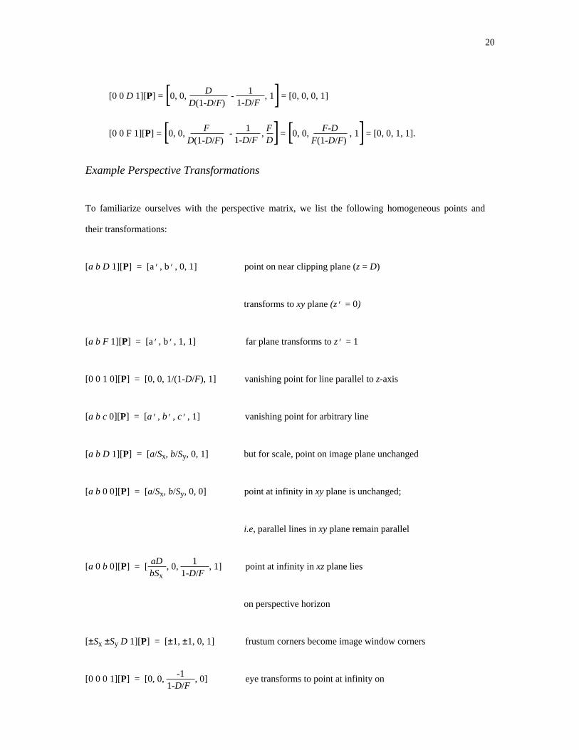
Example Perspective Transformations
To familiarize ourselves with the perspective matrix, we list the following homogeneous points and
their transformations:
[a b D 1][P] = [a’, b’, 0, 1] point on near clipping plane (z = D)
transforms to xy plane (z’ = 0)
[a b F 1][P] = [a’, b’, 1, 1] far plane transforms to z’ = 1
[0 0 1 0][P] = [0, 0, 1/(1-D/F), 1] vanishing point for line parallel to z-axis
[a b c 0][P] = [a’, b’, c’, 1] vanishing point for arbitrary line
[a b D 1][P] = [a/Sx, b/Sy, 0, 1] but for scale, point on image plane unchanged
[a b 0 0][P] = [a/Sx, b/Sy, 0, 0] point at infinity in xy plane is unchanged;
i.e, parallel lines in xy plane remain parallel
[a 0 b 0][P] = [ aDbSx
, 0, 11-D/F
, 1] point at infinity in xz plane lies
on perspective horizon
[±Sx ±Sy D 1][P] = [±1, ±1, 0, 1] frustum corners become image window corners
[0 0 0 1][P] = [0, 0, -11-D/F
, 0] eye transforms to point at infinity on
21
negative perspective z-axis
Associated Vertex Transformations
The efficient shading of a polygon whose vertices have been transformed to the display screen is
usually accomplished by incremental techniques described in the literature [Newman]. Similar
techniques may be applied to vertex parameters such as color and texture. Any parameter
interpolated across a polygon must follow the same transformation as the polygon vertices; if the
transformation includes perspective, a homogeneous division is required at each pixel within the
screen space polygon (in practice, linear interpolation in screen space is usually not objectionable
for parameters such as color, but is often apparent when applied to texture coordinates).
Specifically, for perspective transformations, an interpolated parameter will have the form
(asx+bsy+c)/(dsx+esy+f),
where sx and sy are screen space coordinates. [Heckbert] refers to this as ‘rational linear
interpolation,’ in a detailed discussion of texture coordinate transformations. [Blinn92], which
provides an intuitive review of graphics transformations and homogeneous coordinates, refers to
this as ‘hyperbolic interpolation.’ In the case where the polygon is parallel to the projection plane,
d = e = 0 and the above equation reduces to linear interpolation.
Homogeneous Clipping
Three-dimensional line segments and polygon edges must be clipped to the viewing frustum. This
should be performed in perspective space, after vertex colors have been computed; otherwise,
clipping, by modifying a vertex’s location, would modify its color. By clipping in perspective space
the integrity of the polygon is maintained longer. Also, in homogeneous screen space the
equations for the clipping planes are of the form x = w, whereas they are more complex in object
22
space. [Blinn78, Blinn91] develop this material in greater detail.
In this section we use ‘*’ to represent homogeneous coordinates before the conversion to Euclidean
space. That is, [x*, y*, z*, w*] = [x y z 1][P] and (x’, y’, z’) = (x*/w*, y*/w*, z*/w*).
As shown in Figure 7, the viewing frustum is transformed by the perspective matrix to a
parallelepiped in perspective space, and (x’, y’, z’) is clipped such that -1 ≤ x’, y’ ≤ 1 and 0 ≤
z’ ≤ 1. Note that negative z values result in negative w values, with z’ = z*/w* > 0. Thus,
points behind the eye must be clipped before the homogeneous division. In summary, we test that:
for positive w: for negative w:
-w* ≤ x*, y* -- left, bottom -- -w* ≥ x*, y*
x*, y* ≤ w* -- right, top -- x*, y* ≥ w*
0 ≤ z* -- near -- 0 ≥ z*
z* ≤ w* -- far -- z* ≥ w*
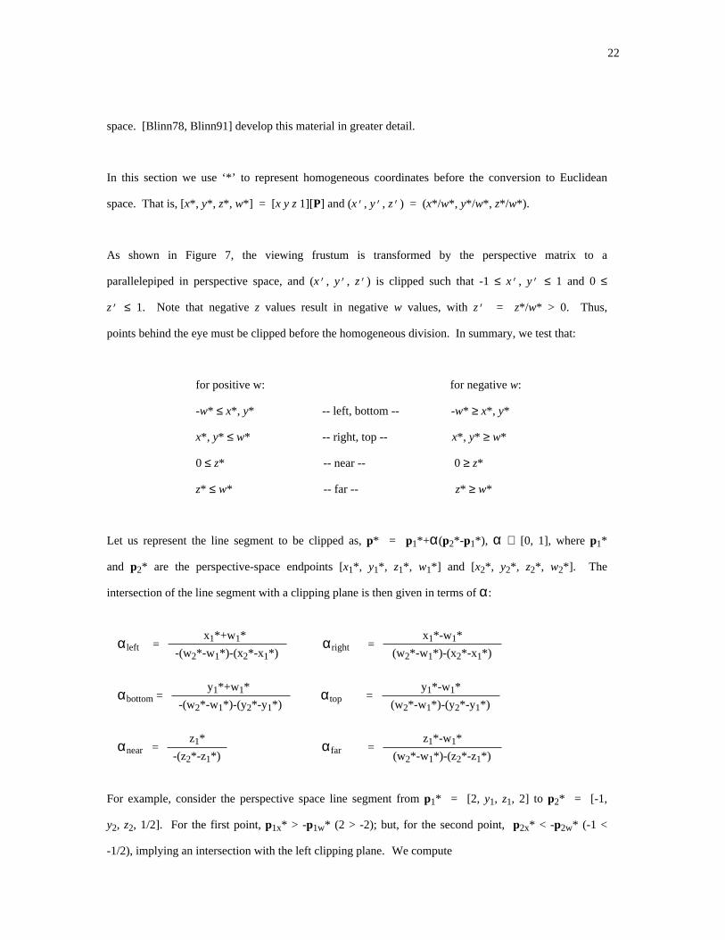
Let us represent the line segment to be clipped as, p* = p1*+α(p2*-p1*), α ∈ [0, 1], where p1*
and p2* are the perspective-space endpoints [x1*, y1*, z1*, w1*] and [x2*, y2*, z2*, w2*]. The
intersection of the line segment with a clipping plane is then given in terms of α:
αleft = x1*+w1*
-(w2*-w1*)-(x2*-x1*)αright =
x1*-w1*
(w2*-w1*)-(x2*-x1*)
αbottom = y1*+w1*
-(w2*-w1*)-(y2*-y1*)αtop =
y1*-w1*
(w2*-w1*)-(y2*-y1*)
αnear = z1*
-(z2*-z1*) αfar =
z1*-w1*
(w2*-w1*)-(z2*-z1*)
For example, consider the perspective space line segment from p1* = [2, y1, z1, 2] to p2* = [-1,
y2, z2, 1/2]. For the first point, p1x* > -p1w* (2 > -2); but, for the second point, p2x* < -p2w* (-1 <
-1/2), implying an intersection with the left clipping plane. We compute
23
αleft = (2+2)/(-(1/2-2)-(-1-2)) = 8/9.
The intersection with the left clipping plane is now given by
p* = [-2/3, y1*+(8/9)(y2*-y1*), z1*+(8/9)(z2*-z1*), 2/3].
The projected x-coordinate of p* = x*/w* = (-2/3)(3/2) = -1, which is the left boundary of
the viewing frustum.
Conclusion
In this paper we have offered a unified view of homogeneous coordinates within a Computer
Graphics context. First, a brief historical review revealed that, as the understanding of perspective
and projections increased, new coordinate systems were developed to represent the underlying
spaces; one of these systems was the homogeneous coordinate system, which was later seen to
possess properties useful for Computer Graphics.
Next, we formally introduced the homogeneous coordinate system. Its application in two-
dimensional Euclidean space was discussed in some detail; it was shown that affine transformations
can be effected consistently with matrix multiplication, thus simplifying sequences of
transformations, and that the intersection of two-dimensional lines can be performed without
special cases.
Homogeneous coordinates in three dimensions were discussed in greater detail, with particular
attention devoted to perspective transformations. Finally, a method to clip lines with respect to the
viewing frustum was provided.
24
Acknowledgements
We gratefully acknowledge Jim Blinn, Charlie Gunn, Paul Heckbert, and Ken Shoemake for
numerous suggestions that improved this paper. We also thank the referees for their thorough
reviews and valuable suggestions, many of which we have incorporated into this paper.
References
Aleksandrov, A.D., Kolmogorov, A.N., Lavientèv, M.A. Mathematics, its Content, Methods and
Meaning. MIT Press, 1969.
Ahuja, D.V. and Coons, S.A. Geometry for Construction and Display. IBM Systems Journal (3, 4),
1968, pp. 188-205.
Ayres, F. Projective Geometry. Schaum Publishing, New York, 1967.
Barsky, B. Rational Beta-splines for Representing Curves and Surfaces. IEEE Computer Graphics
and Applications 13 (6), 1993, pp. 24-32.
Bez, H.E. Homogeneous Coordinates for Computer Graphics. Computer-Aided Design 15 (6),
Nov., 1983, pp. 361-365.
Blinn, J. A Trip down the Graphics Pipeline: the Homogeneous Perspective Transform. IEEE
Computer Graphics and Applications. May, 1993, pp. 75-80.
Blinn, J. A Homogeneous Formulation for Lines in 3 Space. Proceedings of SIGGRAPH 77. In
Computer Graphics 11 (3), 1977.
Blinn, J. A Trip Down the Graphics Pipeline: Line Clipping. IEEE Computer Graphics and
25
Applications 11 (1), 1991, pp. 98-105.
Blinn, J. The Algebraic Properties of Homogeneous Second Order Surfaces. SIGGRAPH Course
Notes (Mathematics of Computer Graphics), 1984.
Blinn, J. Hyberbolic Interpolation. IEEE Computer Graphics and Applications 12 (4), 1992, pp.
89-94.
Blinn, J., Newell, M.E. Clipping Using Homogeneous Coordinates. Proceedings of SIGGRAPH 78.
In Computer Graphics 12 (3), 1978.
Brieskorn, E. and Knörrer, H. Plane Algebraic Curves. Birkhäuser, Basel, 1986.
Carlbom, I. and Paciorek, J. Geometric Projections and Viewing Transformations. ACM Computing
Surveys 10 (4), 1978.
Coxeter, H.S.M. Projective Geometry (second edition), Springer-Verlag, New York, 1987.
Farin, G. Curves and Surfaces for Computer Aided Geometric Design (second edition), Academic
Press, New York, 1990.
Foley, J.D., van Dam, A., Feiner, S.K., Hughes, J.F. Computer Graphics, Principles and Practice
(second edition). Addison Wesley, Reading, Massachusetts, 1990.
Heckbert, P. Fundamentals of Texture Mapping and Image Warping. Masters thesis, Computer
Science Division, The University of California at Berkeley, May, 1989.
Herman, I. The Use of Projective Geometry in Computer Graphics. Lecture Notes in Computer
Science 564, Springer Verlag, 1991.
Kantani, K. Computational Projective Geometry. Computer Vision, Graphics, and Image
26
Processing 54, 1991.
Kline, M. Mathematical Thought from Ancient to Modern Times. Oxford University Press, New
York, 1972.
Möbius, F. Gesammelte Werke, vol. 1, pp. 36-49, Die Barycentrische Calcul. Dr. M. Saendig
oHG, Wiesbaden, Germany, 1967.
Newman, W.M. and Sproull, R.F. Principles of Interactive Computer Graphics. McGraw-Hill,
New York, 1979, pp. 491-501.
Oxford University Press. The Compact Edition of the Oxford English Dictionary. Oxford
University Press, New York, 1971.
Patterson, R.R. Projective Transformations of the Parameter of a Bernstein-Bezier Curve. ACM
Transactions on Graphics, 4, 1985, pp. 276-290.
Pellegrini, M. Ray-shooting and Isotopy Classes of Lines in 3-Dimensional Space. Lecture Notes in
Computer Science 511, Springer Verlag, 1991.
Penna, M.A., Patterson, R.R. Projective Geometry and its Application to Computer Graphics.
Prentice Hall, Englewood Cliffs, N.J., 1986.
Plücker, J. Uber ein neues Coordinatensystem. Journal für die Reine und Angewandte
Mathematick, vol. 5, 1830, pp. 1-36.
Qiulin, D. and Davies, B.J. Surface Geometry for Computer-Aided Design and Manufacture. Ellis
Horwood, Chichester, 1987.
Riesenfeld, R.F. Homogeneous Coordinates and Projective Planes in Computer Graphics. IEEE
27
Computer Graphics and Applications 1 (1), Jan., 1981, pp. 50-55.
Roberts, L.G. Homogeneous matrix representation and manipulation of n-dimensional constructs.
MS-1405, Lincoln Laboratory, MIT, May, 1965.
Rogers, D.F., Adams, J.A. Mathematical Elements for Computer Graphics (second edition).
McGraw Hill, New York, 1990.
Ryan, P.J. Euclidean and Non-Euclidean Geometry. Cambridge University Press, Cambridge,
1986.
Snyder, J. and Barr, A. Ray Tracing Complex Models Containing Surface Tessellations.
Proceedings of SIGGRAPH 87. In Computer Graphics 21 (3), 1987.
Stolfi, J. Oriented Projective Geometry. Academic Press, 1991.
Veblen, O. and Young, J.W. A Mathematical Science. In The World of Mathematics, J. Newman,
ed. Simon and Schuster, vol. 3, pp. 1696-1707, 1956.
Recommended

![A key to the projective model of homogeneous metric spaces · homogeneous coordinates [6]. Projective geometry is di erent from a ne geometry in that it also allows one to model points,](https://img.pdfslide.us/doc/110x75/5e4131848c2f1d3aac60e989/a-key-to-the-projective-model-of-homogeneous-metric-spaces-homogeneous-coordinates.jpg)