2. Generalized Homogeneous Coordinates

for Computational Geometry †

HONGBO LI, DAVID HESTENESDepartment of Physics and AstronomyArizona State UniversityTempe, AZ 85287-1504, USA

ALYN ROCKWOODPower Take Off Software, Inc.18375 Highland Estates Dr.Colorado Springs, CO 80908, USA

2.1 Introduction

The standard algebraic model for Euclidean space En is an n-dimensional realvector space Rn or, equivalently, a set of real coordinates. One trouble withthis model is that, algebraically, the origin is a distinguished element, whereasall the points of En are identical. This deficiency in the vector space modelwas corrected early in the 19th century by removing the origin from the planeand placing it one dimension higher. Formally, that was done by introducinghomogeneous coordinates [H91]. The vector space model also lacks adequaterepresentation for Euclidean points or lines at infinity. We solve both problemshere with a new model for En employing the tools of geometric algebra. We callit the homogeneous model of En.

Our “new model” has its origins in the work of F. A. Wachter (1792–1817),a student of Gauss. He showed that a certain type of surface in hyperbolicgeometry known as a horosphere is metrically equivalent to Euclidean space, soit constitutes a non-Euclidean model of Euclidean geometry. Without knowl-edge of this model, the technique of comformal and projective splits needed toincorporate it into geometric algebra were developed by Hestenes in [H91]. Theconformal split was developed to linearize the conformal group and simplify theconnection to its spin representation. The projective split was developed to in-corporate all the advantages of homogeneous coordinates in a “coordinate-free”representation of geometrical points by vectors.

Andraes Dress and Timothy Havel [DH93] recognized the relation of theconformal split to Wachter’s model as well as to classical work on distancegeometry by Menger [M31], Blumenthal [B53, 61] and Seidel [S52, 55]. Theyalso stressed connections to classical invaraint theory, for which the basics havebeen incorporated into geometric algebra in [HZ91] and [HS84]. The presentwork synthesizes all these developments and integrates conformal and projectivesplits into a powerful algebraic formalism for representing and manipulating

† This work has been partially supported by NSF Grant RED-9200442.

1

geometric concepts. We demonstrate this power in an explicit construction ofthe new homogeneous model of En, the characterization of geometric objectstherein, and in the proofs of geometric theorems.

The truly new thing about our model is the algebraic formalism in which itis embedded. This integrates the representational simplicity of synthetic geom-etry with the computational capabilities of analytic geometry. As in syntheticgeometry we designate points by letters a, b, . . . , but we also give them alge-braic properties. Thus, the outer product a ∧ b represents the line determinedby a and b. This notion was invented by Hermann Grassmann [G1844] andapplied to projective geometry, but it was incorporated into geometric algebraonly recently [HZ91]. To this day, however, it has not been used in Euclideangeometry, owing to a subtle defect that is corrected by our homogeneous model.We show that in our model a ∧ b ∧ c represents the circle through the threepoints. If one of these points is a null vector e representing the point at infinity,then a ∧ b ∧ e represents the straight line through a and b as a circle throughinfinity. This representation was not available to Grassmann, because he didnot have the concept of null vector.

Our model also solves another problem that perplexed Grassmann thoughouthis life. He was finally forced to conclude that it is impossible to define ageometrically meaningful inner product between points. The solution eludedhim because it requires the concept of indefinite metric that accompanies theconcept of null vector. Our model supplies an inner product a · b that directlyrepresents the Euclidean distance between the points. This is a boon to distancegeometry, because it greatly facilitates computation of distances among manypoints. Havel [H98] has used this in applications of geometric algebra to thetheory of molecular conformations. The present work provides a framework forsignificantly advancing such applications.

We believe that our homogeneous model provides the first ideal frameworkfor computational Euclidean geometry. The concepts and theorems of syntheticgeometry can be translated into algebraic form without the unnecessary com-plexities of coordinates or matrices. Constructions and proofs can be done bydirect computations, as needed for practical applications in computer vision andsimilar fields. The spin representation of conformal transformations greatly fa-cilitates their composition and application. We aim to develop the basics andexamples in sufficient detail to make applications in Euclidean geometry fairlystraightforward. As a starting point, we presume familiarity with the notationsand results of Chapter 1.

We have confined our analysis to Euclidean geometry, because it has thewidest applicability. However, the algebraic and conceptual framework appliesto geometrics of any signature. In particular, it applies to modeling spacetimegeometry, but that is a matter for another time.

2

2.2 Minkowski Space with Conformal and

Projective Splits

The real vector space Rn,1 (or R1,n) is called a Minkowski space, after the manwho introduced R3,1 as a model of spacetime. Its signature (n, 1) (1, n) iscalled the Minkowski signature. The orthogonal group of Minkowski space iscalled the Lorentz group, the standard name in relativity theory. Its elementsare called Lorentz transformations. The special orthogonal group of Minkowskispace is called the proper Lorentz group, though the adjective “proper” is oftendropped, especially when reflections are not of interest. A good way to removethe ambiguity is to refer to rotations in Minkowski space as proper Lorentzrotations composing the proper Lorentz rotation group.

As demonstrated in many applications to relativity physics (beginning with[H66]) the “Minkowski algebra” Rn,1 = G(Rn,1) is the ideal instrument forcharacterizing geometry of Minkowski space. In this paper we study its surpris-ing utility for Euclidean geometry. For that purpose, the simplest Minkowskialgebra R1,1 plays a special role.

The Minkowski plane R1,1 has an orthonormal basis {e+, e−} defined by theproperties

e2± = ±1 , e+ · e− = 0 . (2.1)

A null basis {e0, e} can be introduced by

e0 = 12 (e− − e+) , (2.2a)

e = e− + e+ . (2.2b)

Alternatively, the null basis can be defined directly in terms of its properties

e20 = e2 = 0 , e · e0 = −1 . (2.3)

A unit pseudoscalar E for R1,1 is defined by

E = e ∧ e0 = e+ ∧ e− = e+ e− . (2.4)

We note the properties

E2 = 1 , E† = −E , (2.5a)Ee± = e∓ , (2.5b)Ee = −eE = −e , Ee0 = −e0E = e0 , (2.5c)1 − E = −ee0 , 1 + E = −e0e . (2.5d)

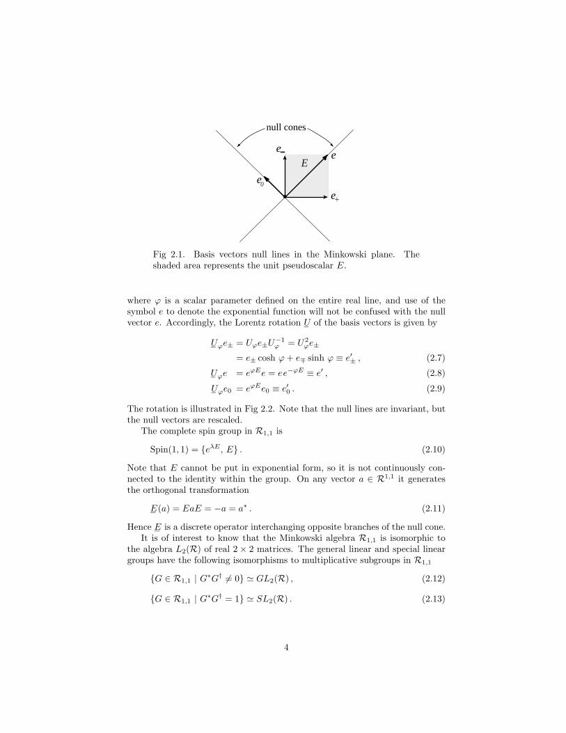
The basis vectors and null lines in R1,1 are illustrated in Fig. 2.1. It will beseen later that the asymmetry in our labels for the null vectors corresponds toan asymmetry in their geometric interpretation.

The Lorentz rotation group for the Minkowski plane is represented by therotor

Uϕ = e12 ϕE , (2.6)

3

.

e

e+

e0

e-

null cones

E

Fig 2.1. Basis vectors null lines in the Minkowski plane. Theshaded area represents the unit pseudoscalar E.

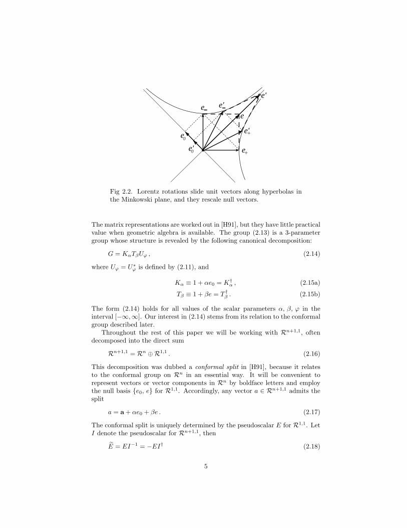
where ϕ is a scalar parameter defined on the entire real line, and use of thesymbol e to denote the exponential function will not be confused with the nullvector e. Accordingly, the Lorentz rotation U of the basis vectors is given by

Uϕe± = Uϕe±U−1ϕ = U2

ϕe±

= e± cosh ϕ + e∓ sinh ϕ ≡ e′± , (2.7)

Uϕe = eϕEe = ee−ϕE ≡ e′ , (2.8)

Uϕe0 = eϕEe0 ≡ e′0 . (2.9)

The rotation is illustrated in Fig 2.2. Note that the null lines are invariant, butthe null vectors are rescaled.

The complete spin group in R1,1 is

Spin(1, 1) = {eλE , E} . (2.10)

Note that E cannot be put in exponential form, so it is not continuously con-nected to the identity within the group. On any vector a ∈ R1,1 it generatesthe orthogonal transformation

E(a) = EaE = −a = a∗ . (2.11)

Hence E is a discrete operator interchanging opposite branches of the null cone.It is of interest to know that the Minkowski algebra R1,1 is isomorphic to

the algebra L2(R) of real 2 × 2 matrices. The general linear and special lineargroups have the following isomorphisms to multiplicative subgroups in R1,1

{G ∈ R1,1 | G∗G† �= 0} � GL2(R) , (2.12)

{G ∈ R1,1 | G∗G† = 1} � SL2(R) . (2.13)

4

.

e

e+

e0

e-

e'+

e'

e'0

e'-

Fig 2.2. Lorentz rotations slide unit vectors along hyperbolas inthe Minkowski plane, and they rescale null vectors.

The matrix representations are worked out in [H91], but they have little practicalvalue when geometric algebra is available. The group (2.13) is a 3-parametergroup whose structure is revealed by the following canonical decomposition:

G = KαTβUϕ , (2.14)

where Uϕ = U∗ϕ is defined by (2.11), and

Kα ≡ 1 + αe0 = K†α , (2.15a)

Tβ ≡ 1 + βe = T †β . (2.15b)

The form (2.14) holds for all values of the scalar parameters α, β, ϕ in theinterval [−∞,∞]. Our interest in (2.14) stems from its relation to the conformalgroup described later.

Throughout the rest of this paper we will be working with Rn+1,1, oftendecomposed into the direct sum

Rn+1,1 = Rn ⊕R1,1 . (2.16)

This decomposition was dubbed a conformal split in [H91], because it relatesto the conformal group on Rn in an essential way. It will be convenient torepresent vectors or vector components in Rn by boldface letters and employthe null basis {e0, e} for R1,1. Accordingly, any vector a ∈ Rn+1,1 admits thesplit

a = a + αe0 + βe . (2.17)

The conformal split is uniquely determined by the pseudoscalar E for R1,1. LetI denote the pseudoscalar for Rn+1,1, then

E = EI−1 = −EI† (2.18)

5

is a unit pseudoscalar for Rn, and we can express the split as

a = PE(a) + P⊥E (a) , (2.19)

where the projection operators PE and P⊥E are given by

PE(a) = (a · E)E = αe0 + βe ∈ R1,1 , (2.20a)

P⊥E (a) = (a · E)E† = (a ∧ E)E = a ∈ Rn . (2.20b)

The Minkowski plane for R1,1 is referred to as the E-plane, since, as (2.20b)shows, it is uniquely determined by E. The projection P⊥

E can be regarded asa rejection from the E-plane.

It is worth noting that the conformal split was defined somewhat differentlyin [H91]. There the points a in Rn were identified with trivectors (a ∧ E)Ein (2.20b). Each of these two alternatives has its own advantages, but theirrepresentations of Rn are isomorphic, so the choice between them is a minormatter of convention.

The idea underlying homogeneous coordinates for “points” in Rn is to removethe troublesome origin by embedding Rn in a space of higher dimension. Anefficient technique for doing this with geometric algebra is the projective splitintroduced in [H91]. We use it here as well. Let e be a vector in the E-plane.Then for any vector a ∈ Rn+1,1 with a · e �= 0, the projective split with respectto e is defined by

ae = a · e + a ∧ e = a · e(1 +

a ∧ e

a · e)

. (2.21)

This represents vector a with the bivector a ∧ e/a · e. The representation isindependent of scale, so it is convenient to fix the scale by the condition a ·e = e0 · e = −1. This condition does not affect the components of a in Rn.Accordingly, we refer to e∧ a = −a∧ e as a projective representation for a. Theclassical approach to homogeneous coordinates corresponds to a projective splitwith respect to a non-null vector. We shall see that there are great advantagesto a split with respect to a null vector. The result is a kind of “generalized”homogeneous coordinates.

A hyperplane Pn+1(n, a) with normal n and containing point a is the solutionset of the equation

n · (x − a) = 0 , x ∈ Rn+1,1 . (2.22)

As explained in Chapter 1, this can be alternatively described by

n ∧ (x − a) = 0 , x ∈ Rn+1,1 . (2.23)

where n = nI−1 is the (n + 1)-vector dual to n.The “normalization condition” x · e = e · e0 = −1 for a projective split with

respect to the null vector e is equivalent to the equation e · (x− e0) = 0; thus xlie on the hyperplane

Pn+1(e, e0) = {x ∈ Rn+1,1 | e · (x − e0) = 0} . (2.24)

6

This fulfills the primary objective of homogeneous coordinates by displacing theorigin of Rn by e0. One more condition is needed to fix x as representation fora unique x in Rn.

2.3 Homogeneous Model of Euclidean Space

The set Nn+1 of all null vectors in Rn+1,1 is called the null cone. We com-plete our definition of generalized homogeneous coordinates for points in Rn byrequiring them to be null vectors, and lie in the intersection of Nn+1 with thehyperplane Pn+1(e, e0) defined by (2.24). The resulting surface

N ne = Nn+1 ∩ Pn+1(e, e0) = {x ∈ Rn+1,1 | x2 = 0, x · e = −1} (2.25)

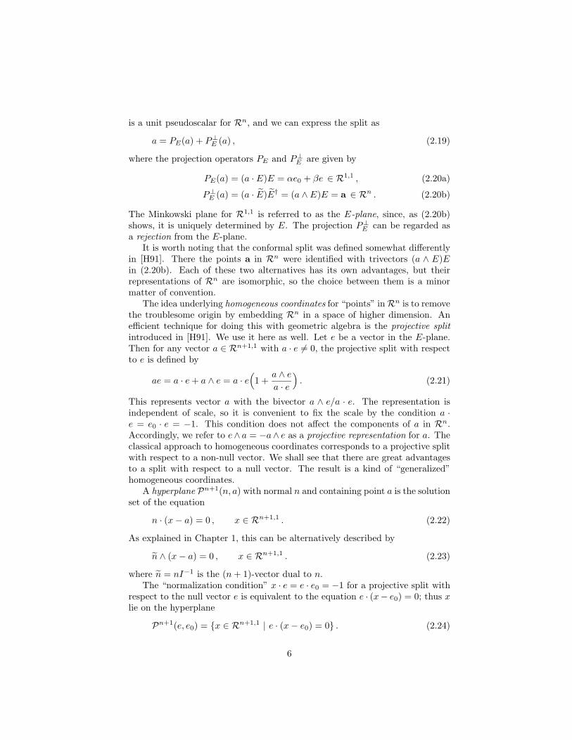
is a parabola in R2,1, and its generalization to higher dimensions is called ahorosphere in the literature on hyperbolic geometry. Applying the conditionsx2 = 0 and x · e = −1 to determine the parameters in (2.17), we get

x = x + 12x

2e + e0 . (2.26)

This defines a bijective mapping of x ∈ Rn to x ∈ Nne . Its inverse is the

rejection (2.20b). Its projection onto the E-plane (2.20a) is shown in Fig. 2.3.Since Rn is isomorphic to En, so is Nn

e , and we have proved

Theorem 1

En � Nne � Rn . (2.27)

We call Nne the homogeneous model of En (or Rn), since its elements are (gen-

eralized) homogeneous coordinates for points in En (or Rn). In view of theirisomorphism, it will be convenient to identify Nn

e with En and refer to the ele-ments of N n

e simply as (homogeneous) points. The adjective homogeneous willbe employed when it is necessary to distinguish these points from points in Rn,which we refer to as inhomogeneous points. Our notations x and x in (2.26) areintended to maintain this distinction.

We have framed our discussion in terms of “homogeneous coordinates” be-cause that is a standard concept. However, geometric algebra enables us tocharacterize a point as a single vector without ever decomposing a vector into aset of coordinates for representational or computational purposes. It is prefer-able, therefore, to speak of “homogeneous points” rather than “homogeneouscoordinates.”

By setting x = 0 in (2.26) we see that e0 is the homogeneous point corre-sponding to the origin of Rn. From

x

−x · e0= e + 2

(x + e0

x2

)−−−−−→x2→∞ e , (2.28)

we see that e represents the point at infinity.

7

. e

e0

x

horosphere x + ee0 + x2–2

1

Fig 2.3. The horosphere Nne and its projection onto the E-plane.

As introduced in (2.21), the projective representation for the point (2.26) is

e ∧ x =e ∧ x

−e · x = ex + e ∧ e0 . (2.29)

Note that e ∧ x = ex = −xe since e · x = 0. By virtue of (2.5a) and (2.5c),

(e ∧ x) E = 1 + ex . (2.30)

This is identical to the representation for a point in the affine model of En intro-duced in Chapter 1. Indeed, the homogeneous model maintains and generalizesall the good features of the affine model.

Lines, planes and simplexes

Before launching into a general treatment of geometric objects, we considerhow the homogeneous model characterizes the simplest objects and relationsin Euclidean geometry. Using (2.26) we expand the geometric product of twopoints a and b as

ab = ab+(a−b)e0 − 12

[(a2 + b2) + (ba2 − ab2)e + (b2 − a2)E

].(2.31)

From the bivector part we get

e ∧ a ∧ b = e ∧ (a + e0) ∧ (b + e0) = ea ∧ b + (b − a)E . (2.32)

From Chapter 1, we recognize a ∧ b = a ∧ (b − a) as the moment for a linethrough point a with tangent a−b, so e∧a∧b characterizes the line completely.

8

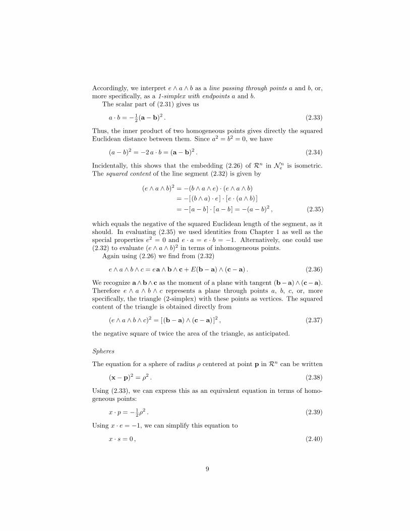
Accordingly, we interpret e ∧ a ∧ b as a line passing through points a and b, or,more specifically, as a 1-simplex with endpoints a and b.

The scalar part of (2.31) gives us

a · b = − 12 (a − b)2 . (2.33)

Thus, the inner product of two homogeneous points gives directly the squaredEuclidean distance between them. Since a2 = b2 = 0, we have

(a − b)2 = −2 a · b = (a − b)2 . (2.34)

Incidentally, this shows that the embedding (2.26) of Rn in Nne is isometric.

The squared content of the line segment (2.32) is given by

(e ∧ a ∧ b)2 = −(b ∧ a ∧ e) · (e ∧ a ∧ b)= −[ (b ∧ a) · e ] · [e · (a ∧ b) ]

= −[a − b ] · [a − b ] = −(a − b)2 , (2.35)

which equals the negative of the squared Euclidean length of the segment, as itshould. In evaluating (2.35) we used identities from Chapter 1 as well as thespecial properties e2 = 0 and e · a = e · b = −1. Alternatively, one could use(2.32) to evaluate (e ∧ a ∧ b)2 in terms of inhomogeneous points.

Again using (2.26) we find from (2.32)

e ∧ a ∧ b ∧ c = ea ∧ b ∧ c + E(b − a) ∧ (c − a) . (2.36)

We recognize a∧b∧ c as the moment of a plane with tangent (b−a)∧ (c−a).Therefore e ∧ a ∧ b ∧ c represents a plane through points a, b, c, or, morespecifically, the triangle (2-simplex) with these points as vertices. The squaredcontent of the triangle is obtained directly from

(e ∧ a ∧ b ∧ c)2 = [(b − a) ∧ (c − a) ]2 , (2.37)

the negative square of twice the area of the triangle, as anticipated.

Spheres

The equation for a sphere of radius ρ centered at point p in Rn can be written

(x − p)2 = ρ2 . (2.38)

Using (2.33), we can express this as an equivalent equation in terms of homo-geneous points:

x · p = −12ρ2 . (2.39)

Using x · e = −1, we can simplify this equation to

x · s = 0 , (2.40)

9

where

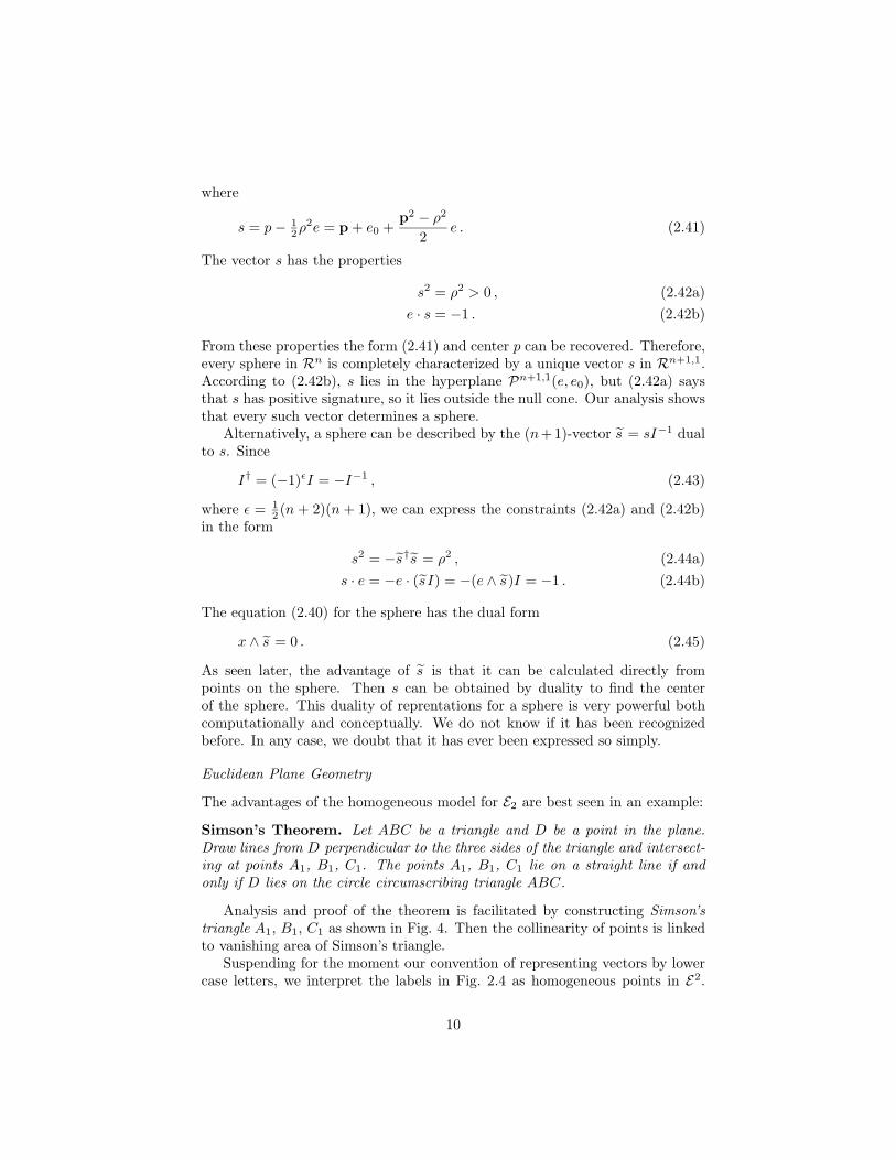
s = p − 12ρ2e = p + e0 +

p2 − ρ2

2e . (2.41)

The vector s has the properties

s2 = ρ2 > 0 , (2.42a)e · s = −1 . (2.42b)

From these properties the form (2.41) and center p can be recovered. Therefore,every sphere in Rn is completely characterized by a unique vector s in Rn+1,1.According to (2.42b), s lies in the hyperplane Pn+1,1(e, e0), but (2.42a) saysthat s has positive signature, so it lies outside the null cone. Our analysis showsthat every such vector determines a sphere.

Alternatively, a sphere can be described by the (n+1)-vector s = sI−1 dualto s. Since

I† = (−1)εI = −I−1 , (2.43)

where ε = 12 (n + 2)(n + 1), we can express the constraints (2.42a) and (2.42b)

in the form

s2 = −s†s = ρ2 , (2.44a)s · e = −e · (sI) = −(e ∧ s)I = −1 . (2.44b)

The equation (2.40) for the sphere has the dual form

x ∧ s = 0 . (2.45)

As seen later, the advantage of s is that it can be calculated directly frompoints on the sphere. Then s can be obtained by duality to find the centerof the sphere. This duality of reprentations for a sphere is very powerful bothcomputationally and conceptually. We do not know if it has been recognizedbefore. In any case, we doubt that it has ever been expressed so simply.

Euclidean Plane Geometry

The advantages of the homogeneous model for E2 are best seen in an example:

Simson’s Theorem. Let ABC be a triangle and D be a point in the plane.Draw lines from D perpendicular to the three sides of the triangle and intersect-ing at points A1, B1, C1. The points A1, B1, C1 lie on a straight line if andonly if D lies on the circle circumscribing triangle ABC.

Analysis and proof of the theorem is facilitated by constructing Simson’striangle A1, B1, C1 as shown in Fig. 4. Then the collinearity of points is linkedto vanishing area of Simson’s triangle.

Suspending for the moment our convention of representing vectors by lowercase letters, we interpret the labels in Fig. 2.4 as homogeneous points in E2.

10

..

...

..

.

A

B C

D

P

A1

C1

B1

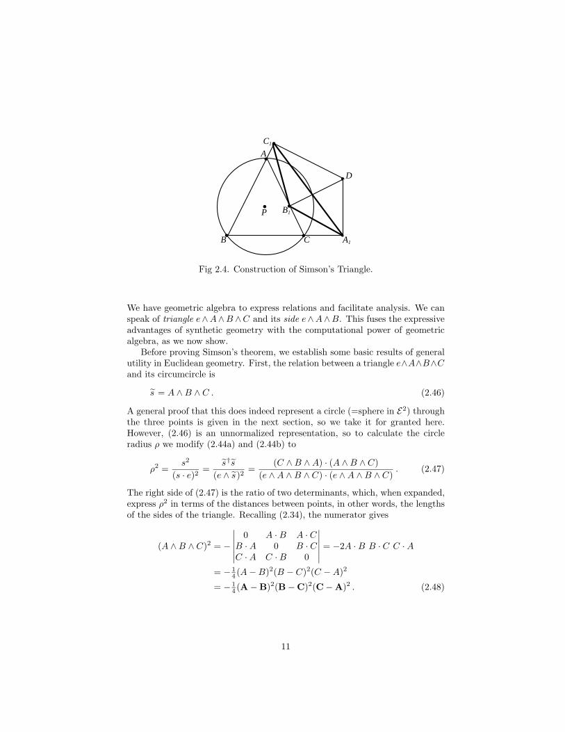
Fig 2.4. Construction of Simson’s Triangle.

We have geometric algebra to express relations and facilitate analysis. We canspeak of triangle e∧A∧B ∧C and its side e∧A∧B. This fuses the expressiveadvantages of synthetic geometry with the computational power of geometricalgebra, as we now show.

Before proving Simson’s theorem, we establish some basic results of generalutility in Euclidean geometry. First, the relation between a triangle e∧A∧B∧Cand its circumcircle is

s = A ∧ B ∧ C . (2.46)

A general proof that this does indeed represent a circle (=sphere in E2) throughthe three points is given in the next section, so we take it for granted here.However, (2.46) is an unnormalized representation, so to calculate the circleradius ρ we modify (2.44a) and (2.44b) to

ρ2 =s2

(s · e)2 =s†s

(e ∧ s)2=

(C ∧ B ∧ A) · (A ∧ B ∧ C)(e ∧ A ∧ B ∧ C) · (e ∧ A ∧ B ∧ C)

. (2.47)

The right side of (2.47) is the ratio of two determinants, which, when expanded,express ρ2 in terms of the distances between points, in other words, the lengthsof the sides of the triangle. Recalling (2.34), the numerator gives

(A ∧ B ∧ C)2 = −

∣∣∣∣∣∣0 A · B A · C

B · A 0 B · CC · A C · B 0

∣∣∣∣∣∣ = −2A · B B · C C · A

= −14 (A − B)2(B − C)2(C − A)2

= −14 (A − B)2(B − C)2(C − A)2 . (2.48)

11

The denominator is obtained from (2.37), which relates it to the area of thetriangle and expands to

(e ∧ A ∧ B ∧ C)2 = −4(area)2

= [(B − A) · (C − A) ]2 − (B − A)2(C − A)2

= [(B − A) · (C − A) ]2 − 4(A · B)2(A · C)2 . (2.49)

By normalizing A∧B ∧C and taking its dual, we find the center P of the circlefrom (2.41); thus

−(A ∧ B ∧ C)∼

(e ∧ A ∧ B ∧ C)∼= P − 1

2ρ2 e . (2.50)

This completes our characterization of the intrinsic properties of a triangle.To relate circle A ∧ B ∧ C to a point D, we use

(A ∧ B ∧ C) ∨ D = (A ∧ B ∧ C)˜ · D = −(A ∧ B ∧ C ∧ D)˜with (2.50) to get

A ∧ B ∧ C ∧ D =ρ2 − δ2

2e ∧ A ∧ B ∧ C , (2.51)

where

δ2 = −2P · D (2.52)

is the squared distance between D and P . According to (2.45), the left side of(2.51) vanishes when D is on the circle, in conformity with δ2 = ρ2 on the rightside of (2.51).

To construct the Simson triangle algebraically, we need to solve the problemof finding the “perpendicular intersection” B1 of point D on line e∧A∧C (Fig.2.4). Using inhomogeneous points we can write the condition for perpendicu-larity as

(B1 − D) · (C − A) = 0 . (2.53)

Therefore

(B1 − D)(C − A) = (B1 − D) ∧ (C − A) = (A − D) ∧ (C − A) .

Dividing by (C − A),

B1 − D = [(A − D) ∧ (C − A) ] · (C − A)−1

= A − D − (A − D) · (C − A)−1(C − A) . (2.54)

Therefore

B1 = A +(D − A) · (C − A)

(C − A)2(C − A) . (2.55)

12

We can easily convert this to a relation among homogeneous points. However,we are only interested here in Simson’s triangle e∧A1∧B1∧C1, which by (2.36)can be represented in the form

e ∧ A1 ∧ B1 ∧ C1 = E(B1 − A1) ∧ (C1 − A1)= E(A1 ∧ B1 + B1 ∧ C1 + C1 ∧ A1) . (2.56)

Calculations are simplified considerably by identifying D with the origin in Rn,which we can do without loss of generality. Then equation (2.52) becomesδ2 = −2P · D = p2. Setting D = 0 in (2.55) and determining the analogousexpressions for A1 and C1, we insert the three points into (2.56) and find, aftersome calculation,

e ∧ A1 ∧ B1 ∧ C1 =( ρ2 − δ2

4ρ2

)e ∧ A ∧ B ∧ C . (2.57)

The only tricky part of the calculation is getting the coefficient on the right sideof (2.57) in the form shown. To do that the expanded form for ρ2 in (2.47) to(2.49) can be used.

Finally, combining (2.57) with (2.51) we obtain the identity

e ∧ A1 ∧ B1 ∧ C1 =A ∧ B ∧ C ∧ D

2ρ2. (2.58)

This proves Simson’s theorem, for the right side vanishes if and only if D is onthe circle, while the left side vanishes if and only if the three points lie on thesame line.

2.4 Euclidean Spheres and Hyperspheres

A hyperplane through the origin is called a hyperspace. A hyperspace Pn+1(s)in Rn+1,1(s) with Minkowski signature is called a Minkowski hyperspace. Itsnormal s must have positive.

Theorem 2 The intersection of any Minkowski hyperspace Pn+1(s) with thehorosphere Nn+1

e (s) � En is a sphere or hyperplane

S(s) = Pn+1(s) ∩Nn+1e (2.59)

in En (or Rn), and every Euclidean sphere or hyperplane can be obtained in thisway. S(s) is a sphere if e · s < 0 or a hyperplane if e · s = 0.

Corollary. Every Euclidean sphere or hyperplane can be represented by a vectors (unique up to scale) with s2 > 0 and s · e ≤ 0.

From our previous discussion we know that the sphere S(s) has radius ρgiven by

ρ2 =s2

(s · e)2 , (2.60)

13

and it is centered at point

p =s

−s · e + 12ρ2 e . (2.61)

Therefore, with the normalization s · e = −1, each sphere is represented by aunique vector. With this normalization, the set {x = P⊥

E (x) ∈ Rn|x · s > 0}represents the interior of the sphere, and we refer to (2.61) as the standard formfor the representation of a sphere by vector s.

To prove Theorem 2, it suffices to analyze the two special cases. These casesare distinguished by the identity

(s · e)2 = (s ∧ e)2 ≥ 0 , (2.62)

which follows from e2 = 0. We have already established that (e · s)2 > 0characterizes a sphere. For the case e · s = 0, we observe that the component ofs in Rn is given by

s = P⊥E (s) = (s ∧ E)E = s + (s · e0)e . (2.63)

Therefore

s = | s |(n + eδ) , (2.64)

where n2 = 1 and δ = s · e0/| s |. Set | s | = 1. The equation for a point x onthe surface S(s) is then

x · s = n · x − δ = 0 . (2.65)

This is the equation for a hyperplane in Rn with unit normal n and signeddistance δ from the origin. Since x · e = 0, the “point at infinity” e lies on S(s).Therefore, a hyperplane En can be regarded as a sphere that “passes through”the point at infinity.

With | s | = 1, we refer to (2.64) as the standard form for representation ofa hyperplane by vector s.

Theorem 3 Given homogeneous points a0, a1, a2, . . . , an “in” En such that

s = a0 ∧ a1 ∧ a2 ∧ · · · ∧ an �= 0 , (2.66)

then the (n + 1)-blade s represents a Euclidean sphere if

(e ∧ s)2 �= 0 . (2.67)

or a hyperplane if

(e ∧ s)2 = 0 . (2.68)

A point x is on the sphere/hyperplane S(s) if and only if

x ∧ s = 0 . (2.69)

14

Since (2.66) is a condition for linear independence, we have the converse theoremthat every S(s) is uniquely determined by n + 1 linearly independent points.

By duality, Theorem 3 is an obvious consequence of Theorem 2 where sis dual to the normal s of the hyperspace Pn+1(s), so it is a tangent for thehyperspace.

For a hyperplane, we can always employ the point at infinity so the condition(2.66) becomes

s = e ∧ a1 ∧ a2 ∧ · · · ∧ an �= 0 . (2.70)

Therefore only n linearly independent finite points are needed to define a hy-perplane in En.

2.5 r-dimensional Spheres, Planes and Simplexes

We have seen that (n + 1)-blades of Minkowski signature in Rn+1,1 representspheres and hyperplanes in Rn, so the following generalization is fairly obvious

Theorem 4 For 2 ≤ r ≤ n + 1, every r-blade Ar of Minkowski signature inRn+1,1 represents an (r − 2)-dimensional sphere in Rn (or En).

There are three cases to consider:

Case 1. e∧Ar = e0 ∧Ar = 0, Ar represents an (r− 2)-plane through the originin Rn with standard form

Ar = EIr−2 , (2.71)

where Ir−2 is unit tangent for the plane.

Case 2. Ar represents an (r − 2)-plane when e ∧ Ar = 0 and

Ar+1 = e0 ∧ Ar �= 0 . (2.72)

We can express Ar as the dual of a vector s with respect to Ar+1:

Ar = sAr+1 = (−1)ε s ∨ Ar+1 . (2.73)

In this case e · s = 0 but s · e0 �= 0, so we can write s in the standard forms = n + δe for the hyperplane s with unit normal n in Rn and n-distance δfrom the origin. Normalizing Ar+1 to unity, we can put Ar into the standardform

Ar = (n + eδ)EIr−1 = EnIr−1 + eδIr−1 . (2.74)

This represents an (r−2)-plane with unit tangent nIr−1 = n ·Ir−1 and momentδIr−1. Its directance from the origin is the vector δn.

15

As a corollary to (2.74), the r-plane passing through point a in Rn with unitr-blade Ir as tangent has the standard form

Ar+1 = e ∧ a ∧ Ir , (2.75)

where a = P⊥E (a) is the inhomogeneous point.

Case 3. Ar represents an (r − 2)-dimensional sphere if

Ar+1 ≡ e ∧ Ar �= 0 . (2.76)

The vector

s = ArA−1r+1 (2.77)

has positive square and s · e �= 0, so its dual s = sI−1 represents an (n − 1)-dimensional sphere

Ar = sAr+1 = (sI) · Ar+1 = (−1)ε s ∨ Ar+1 , (2.78)

where the (inessential) sign is determined by (2.43). As shown below, condition(2.76) implies that Ar+1 represents an (r − 1)-plane in Rn. Therefore the meetproduct s ∨ Ar+1 in (2.78) expresses the (r − 2)-sphere Ar as the intersectionof the (n − 1)-sphere s with the (r − 1)-plane Ar+1.

With suitable normalization, we can write s = c− 12ρ2 e where c is the center

and ρ is the radius of sphere s . Since s ∧ Ar+1 = e ∧ Ar+1 = 0, the sphere Ar

is also centered at point c and has radius ρ.Using (2.74) for the standard form of Ar+1, we can represent an (r−2)-sphere

on a plane in the standard form

Ar = (c − 12ρ2e) ∧ (n + eδ)EIr , (2.79)

where | Ir | = 1, c ∧ Ir = n ∧ Ir = 0 and c · n = δ.In particular, we can represent an (r − 2)-sphere in a space in the standard

form

Ar = (c − 12ρ2 e)EIr−1 , (2.80)

where E = e ∧ e0 and Ir−1 is a unit (r − 1)-blade in Rn. In (2.80) the factorEIr−1 has been normalized to unit magnitude. Both (2.78) and (2.80) expressAr as the dual of vector s with respect to Ar+1. Indeed, for r = n + 1, In isa unit pseudoscalar for Rn, so (2.78) and (2.80) give the dual form s that wefound for spheres in the preceding section.

This completes our classification of standard representations for spheres andplanes in En.

16

Simplexes and spheres

Now we examine geometric objects determined by linearly independent homoge-neous points a0, a1, . . . , ar, with r ≤ n so that a0∧a1∧· · ·∧ar �= 0. Introducinginhomogeneous points by (2.26), a simple computation gives the expanded form

a0 ∧ a1 ∧ · · · ∧ ar = Ar + e0A+r + 1

2eA−r − 1

2EA±r , (2.81)

where, for want of a better notation,

Ar = a0 ∧ a1 ∧ · · · ∧ ar,

A+r =

r∑i=0

(−1)ia0 ∧ · · · ∧ ai ∧ · · · ∧ ar = (a1 − a0) ∧ · · · ∧ (ar − a0),

A−r =

r∑i=0

(−1)ia2i a0 ∧ · · · ∧ ai ∧ · · · ∧ ar,

A±r =

r∑i=0

r∑j=i+1

(−1)i+j(a2i − a2

j )a0 ∧ · · · ∧ ai ∧ · · · ∧ aj ∧ · · · ∧ ar.

(2.82)

Theorem 5 The expanded form (2.81)

(1) determines an r-simplex if Ar �= 0,

(2) represents an (r−1)-simplex in a plane through the origin if A+r = A−

r = 0,

(3) represents an (r − 1)-sphere if and only if A+r �= 0.

We establish and analyze each of these three cases in turn.From our study of simplexes in Chapter 1, we recognize Ar as the moment

of a simplex with boundary (or tangent) A+r . Therefore,

e ∧ a0 ∧ a1 ∧ · · · ∧ ar = eAr + EA+r (2.83)

represents an r-simplex. The volume (or content) of the simplex is k! |A+r |,

where

|A+r |2 = (A+

r )†A+r = −(ar ∧ · · · ∧ a0 ∧ e) · (e ∧ a0 ∧ · · · ∧ ar)

= −(− 12 )r

∣∣∣∣∣∣∣∣∣

0 1 · · · 11... d2

ij

1

∣∣∣∣∣∣∣∣∣(2.84)

and dij = |ai − aj | is the pairwise interpoint distance. The determinant on theright side of (2.84) is called the Cayley-Menger determinant, because Cayley

17

found it as an expression for volume in 1841, and nearly a century later Menger[M31] used it to reformulate Euclidean geometry with the notion of interpointdistance as a primitive.

Comparison of (2.83) with (2.74) gives the directed distance from the originin Rn to the plane of the simplex in terms of the points:

δn = Ar(A+r )−1 . (2.85)

Therefore, the squared distance is given by the ratio of determinants:

δ2 =|Ar |2

|A+r |2

=(ar ∧ · · · ∧ a0) · (a0 ∧ · · · ∧ ar)(a r ∧ · · · ∧ a 1) · (a 1 ∧ · · · ∧ a r)

, (2.86)

where a i = ai − a0 for i = 1, . . . , r, and the denominator is an alternative to(2.84).

When A+r = A−

r = 0, (2.81) reduces to

a0 ∧ · · · ∧ ar = −12EA±

r . (2.87)

Comparing with (2.83) we see that this degenerate case represents an (r − 1)-simplex with volume 1

2k!|A±r | in an (r − 1)-plane through the origin. To get

an arbitrary (r − 1)-simplex from a0 ∧ · · · ∧ ar we must place one of the points,say a0, at ∞. Then we have e ∧ a1 ∧ a2 ∧ · · · ∧ ar, which has the same form as(2.83).

We get more insight into the expanded form (2.81) by comparing it with thestandard forms (2.79), (2.80) for a sphere. When Ar = 0, then A+

r �= 0 fora0 ∧ · · · ∧ ar to represent a sphere. Since

a0 ∧ · · · ∧ ar = −[e0 − 12eA−

r (A+r )−1 + 1

2A±r (A+

r )−1 ]EA+r ,

we find that the sphere is in the space represented by EA+r , with center and

squared radius

c = 12A

±r (A+

r )−1 , (2.88a)

ρ2 = c2 + A−r (A+

r )−1 . (2.88b)

When Ar �= 0, then A+r �= 0 because of (2.92b) below. Since

a0 ∧ · · · ∧ ar =(Ar + e0A+

r + 12eA−

r − 12EA±

r )(eAr + EA+r )†

(eAr + EA+r )†(eAr + EA+

r )(eAr + EA+

r ) ,

and the numerator equals

A+r (A+

r )†[e0 +

2A+r (Ar)† + A±

r (A+r )†

2A+r (A+

r )†+

2Ar(Ar)† − A−r (A+

r )†

2A+r (A+

r )†e

],

we find that the sphere is on the plane represented by eAr + EA+r , with center

and squared radius

c =2(A+

r )−1(Ar)† + A±r (A+

r )†

2A+r (A+

r )†, (2.89a)

ρ2 = c2 +A−

r (A+r )† − 2Ar(Ar)†

A+r (A+

r )†. (2.89b)

18

We see that (2.89a), (2.89b) congrue with (2.88a), (2.88b) when Ar = 0.Having shown how the expanded form (2.81) represents spheres or planes of

any dimension, let us analyze relation among the A’s. In (2.82) A+r is already

represented as a blade; when ai �= 0 for all i, the analogous representation forA−

r is

A−r = Πr(a−1

1 − a−10 ) ∧ (a−1

2 − a−10 ) ∧ · · · ∧ (a−1

r − a−10 ) , (2.90)

where

Πr = a20a2

1 · · · a2r . (2.91)

From this we see that A+r and A−

r are interchanged by inversions ai → a−1i , of

all inhomogeneous points.Using the notation for the boundary of a simplex from Chapter 1, we have

A+r = /∂Ar , A−

r /Πr = /∂(Ar/Πr) , (2.92a)A±

r = −/∂A−r , A±

r /Πr = /∂(A+r /Πr) . (2.92b)

An immediate corollary is that all A’s are blades, and if A±r = 0 then all other

A’s are zero.If Ar �= 0, then we have the following relation among the four A’s:

A+r ∨ A−

r = −ArA±r , (2.93)

where the meet and dual are defined in G(Ar). Hence when Ar �= 0, the vectorspaces defined by A+

r and A−r intersect and the intersection is the vector space

defined by A±r .

Squaring (2.81) we get

| a0 ∧ · · · ∧ ar |2 = det(ai · aj) = (− 12 )r+1 det(|ai − aj |2)

= |Ar |2 − (A+r )† · A−

r − 14 |A

±r |2 . (2.94)

For r = n + 1, Ar vanishes and we obtain

Ptolemy’s Theorem: Let a0, a1, . . . , an+1 be points in Rn, then they are ona sphere or a hypersphere if and only if det(|ai − aj |2)(n+2)×(n+2) = 0.

2.6 Relation among Spheres and Hyperplanes

In Section 4 we learned that every sphere or hyperplane in En is uniquely rep-resented by some vector s with s2 > 0 or by its dual s . It will be convenient,therefore, to use s or s as names for the surface they represent. We also learnedthat spheres and hyperplanes are distinguished, respectively, by the conditionss · e > 0 and s · e = 0, and the latter tells us that a hyperplane can be regardedas a sphere through the point at infinity. This intimate relation between spheresand hyperplanes makes it easy to analyze their common properties.

19

A main advantage of the representation by s and s is that it can be useddirectly for algebraic characterization of both qualitative and quantitative prop-erties of surfaces without reference to generic points on the surfaces. In thissection we present important examples of qualitative relations among spheresand hyperplanes that can readily be made quantitative. The simplicity of theserelations and their classifications should be of genuine value in computationalgeometry, especially in problems of constraint satisfaction.

Intersection of spheres and hyperplanes

Let s1 and s2 be two different spheres or hyperplanes of Rn (or En). Both s1

and s2 are tangent (n + 1)-dimensional Minkowski subspaces of Rn+1,1. Thesesubspaces intersect in an n-dimensional subspace with n-blade tangent givenalgebraically by the meet product s1 ∨ s2 defined in Chapter 1. This illustrateshow the homogeneous model of En reduces the computations of intersectionsof spheres and planes of any dimension to intersections of linear subspaces inRn+1,1, which are computed with the meet product.

To classify topological relations between two spheres or hyperplanes, it willbe convenient to work with the dual of the meet:

(s1 ∨ s2)∼ = s1 ∧ s2 . (2.95)

There are three cases corresponding to the possible signatures of s1 ∧ s2:

Theorem 6 Two spheres or hyperplanes s1, s2 intersect, are tangent or par-allel, or do not intersect if and only if (s1 ∧ s2)2 <, =, > 0, respectively.

Let us examine the various cases in more detail.When s1 and s2 are both spheres, then

• if they intersect, the intersection (s1∧s2)∼ is a sphere, as e∧(s1∧s2)∼ �= 0.The center and radius of the intersection are the same with those of thesphere (Ps1∧s2(e))

∼. The intersection lies on the hyperplane (e·(s1∧s2))∼.

• if they are tangent, the tangent point is proportional to the null vectorP⊥

s1(s2) = (s2 ∧ s1)s−1

1 .

• if they do not intersect, there are two points a, b ∈ Rn, called Ponceletpoints [S88], which are inversive to each other with respect to both spheress1 and s2. The reason is, since s1 ∧ s2 is Minkowski, it contains twononcollinear null vectors |s1 ∧ s2|s1 ± |s1|s2|P⊥

s1(s2), which correspond to

a,b ∈ Rn respectively. Let si = λia + µib, where λi, µi are scalars.Then the inversion of a homogeneous point a with respect to the spheresi gives the point si a = (−µi/λi)b, as shown in the section on conformaltransformations.

When s1 is a hyperplane and s2 is a sphere, then

20

• if they intersect, the intersection (s1∧s2)∼ is a sphere, since e∧(s1∧s2)∼ �=0. The center and radius of the intersection are the same with those ofthe sphere (P⊥

s1(s2))∼.

• if they are tangent, the tangent point corresponds to the null vectorP⊥

s1(s2).

When a sphere s and a point a on it is given, the tangent hyperplane ofthe sphere at a is (s + s · ea)∼.

• if they do not intersect, there are two points a, b ∈ Rn as before, calledPoncelet points [S88], which are symmetric with respect to the hyperplanes1 and also inversive to each other with respect to the sphere s2.

When s1 and s2 are both hyperplanes, they always intersect or are parallel, as(s1 ∧ s2)∼ always contains e, and therefore cannot be Euclidean. For the twohyperplanes,

• if they intersect, the intersection (s1∧s2)∼ is an (n−2)-plane. When boths1 and s2 are hyperspaces, the intersection corresponds to the (n − 2)-space (s1 ∧ s2)In in Rn, where Ir is a unit pseudoscalar of Rn; otherwisethe intersection is in the hyperspace (e0 · (s1 ∧ s2))∼ and has the samenormal and distance from the origin as the hyperplane (Ps1∧s2(e0))∼.

• if they are parallel, the distance between them is |e0 · P⊥s2

(s1)|/|s1|.

Now let us examine the geometric significance of the inner product s1 ·s2. Forspheres and hyperspaces s1, s2, the scalar s1 · s2/|s1||s2| is called the inversiveproduct [I92] and denoted by s1 ∗ s2. Obviously, it is invariant under orthogonaltransformations in Rn+1,1, and

(s1 ∗ s2)2 = 1 +(s1 ∧ s2)2

s21s

22

. (2.96)

Let us assume that s1 and s2 are normalized to standard form. Following[I92, p. 40, 8.7], when s1 and s2 intersect, let a be a point of intersection, andlet mi, i = 1, 2, be the respective outward unit normal vector of s i at a if it isa sphere, or the negative of the unit normal vector in the standard form of s i ifit is a hyperplane; then

s1 ∗ s2 = m1 · m2. (2.97)

The above conclusion is proved as follows: For i = 1, 2, when s i representsa sphere with standard form si = ci − 1

2ρ2i e where ci is its center, then

s1 ∗ s2 =ρ21 + ρ2

2 − |c1 − c2|22ρ1ρ2

, (2.98)

m1 · m2 =(a − c1)|a − c1|

· (a − c2)|a − c2|

=ρ21 + ρ2

2 − |c1 − c2|22ρ1ρ2

. (2.99)

21

When s2 is replaced by the standard form n2 + δ2e for a hyperplane, then

s1 ∗ s2 =c1 · n2 − δ2

ρ1, (2.100)

m1 · m2 =(a − c1)|a − c1|

· (−n2) =c1 · n2 − δ2

ρ1; (2.101)

For two hyperspheres si = ni + δif ; then

s1 ∗ s2 = n1 · n2, (2.102)m1 · m2 = n1 · n2. (2.103)

An immediate consequence of this result is that orthogonal transformations inRn+1,1 induce angle-preserving transformations in Rn. These are the conformaltransformations discussed in the next section.

Relations among Three Points, Spheres or Hyperplanes

Let s1, s2, s3 be three distinct nonzero vectors of Rn+1,1 with non-negativesquare. Then the sign of

∆ = s1 · s2 s2 · s3 s3 · s1 (2.104)

is invariant under the rescaling s1, s2, s3 → λ1s1, λ2s2, λ3s3, where the λ’s arenonzero scalars. Geometrically, when s2

i > 0, then s i represents either a sphereor a hyperplane; when s2

i = 0, then si represents either a finite point or thepoint at infinity e. So the sign of ∆ describes some geometric relationshipamong points, spheres or hyperplanes. Here we give a detailed analysis of thecase when ∆ < 0.

When the s’s are all null vectors, then ∆ < 0 is always true, as long as notwo of them are linearly dependent.

When s1 = e, s2 is null, and s23 > 0, then ∆ < 0 implies s3 to represent a

sphere. Our previous analysis shows that ∆ < 0 if and only if the point s2 isoutside the sphere s3.

When s1, s2 are finite points and s23 > 0, a simple analysis shows that ∆ < 0

if and only if the two points by s1, s2 are on the same side of the sphere orhyperplane s3.

When s1 = e, s22, s

23 > 0, then ∆ < 0 implies s2, s3 to represent two spheres.

For two spheres with centers c1, c2 and radii ρ1, ρ2 respectively, we say they are(1) near if |c1 −c2|2 < ρ2

1 +ρ22, (2) far if |c1 −c2|2 > ρ2

1 +ρ22, and (3) orthogonal

if |c1 − c2|2 = ρ21 + ρ2

2. According to the first equation of (2.6), ∆ < 0 if andonly if the two spheres s2 and s3 are far.

When s1 is a finite point and s22, s

23 > 0, then

• if s2 and s3 are hyperplanes, then ∆ < 0 implies that they are neitherorthogonal nor identical. When the two hyperplanes are parallel, then∆ < 0 if and only if the point s1 is between the two hyperplanes. When thehyperplanes intersect, then ∆ < 0 if and only if s1 is in the wedge domainof the acute angle in Rn formed by the two intersecting hyperplanes.

22

• if s2 is a hyperplane and s3 is a sphere, then ∆ < 0 implies that they arenon-orthogonal, i.e., the center of the sphere does not lie on the hyper-plane. If the center of a sphere is on one side of a hyperplane, we also saythat the sphere is on that side of the hyperplane. If the point s1 is outsidethe sphere s3, then ∆ < 0 if and only if s1 and the sphere s3 are on thesame side of the hyperplane s2; if the point is inside the sphere s3, then∆ < 0 if and only if the point and the sphere are on opposite sides of thehyperplane.

• if s2, s3 are spheres, then ∆ < 0 implies that they are non-orthogonal. Ifthey are far, then ∆ < 0 if and only if the point s1 is either inside both ofthem or outside both of them. If they are near, then ∆ < 0 if and only ifs1 is inside one sphere and outside the other.

When s1, s2, s3 are all of positive square, then ∆ < 0 implies that no two ofthem are orthogonal or identical.

• If they are all hyperplanes, with normals n1, n2, n3 respectively, then∆ < 0 implies that no two of them are parallel, as the sign of ∆ equalsthat of n1 · n2 n2 · n3 n3 · n1. ∆ < 0 if and only if a normal vector of s1

with its base point at the intersection of the two hyperplanes s2 and s3,has its end point in the wedge domain of the acute angle in Rn formed bythe two intersecting hyperplanes.

• If s1, s2 are hyperplanes and s3 is a sphere, then when the hyperplanesare parallel, ∆ < 0 if and only if the sphere’s center is between the twohyperplanes. When the hyperplanes intersect, ∆ < 0 if and only if thesphere’s center is in the wedge domain of the acute angle in Rn formedby the two intersecting hyperplanes.

• If s1 is a hyperplane and s2, s3 are spheres, then when the two spheres arefar, ∆ < 0 if and only if the spheres are on the same side of the hyperplane.When the spheres are near, ∆ < 0 if and only if they are on opposite sidesof the hyperplane.

• If all are spheres, then either they are all far from each other, or twospheres are far and the third is near to both of them.

Bunches of Spheres and Hyperplanes

In previous sections, we proved that Minkowski subspaces of Rn+1,1 representspheres and planes of various dimensions in Rn. In this subsection we considersubspaces of Rn+1,1 containing only their normals, which are vectors of posi-tive square. Such subspaces are dual to Minkowski hyperspaces that representspheres or hyperplanes. Therefore the tangent blade for a subspace Ar of Rn+1,1

can be used to represent a set of spheres and hyperplanes, where each of them isrepresented by a vector of positive square. Or dually, the dual of Ar representsthe intersection of a set of spheres and hyperplanes.

23

The simplest example is a pencil of spheres and hyperplanes. Let s1, s2

be two different spheres or hyperplanes, then the pencil of spheres/hyperplanesdetermined by them is the set of spheres/hyperplanes (λ1s1 + λ2s2)∼, whereλ1, λ2 are scalars satisfying

(λ1s1 + λ2s2)2 > 0. (2.105)

The entire pencil is represented by the blade A2 = s1 ∧ s2 or its dual (s1 ∧ s2)∼.There are three kinds of pencils corresponding to the three possible signaturesof the blade s1 ∧ s2:

1. Euclidean, (s1 ∧ s2)2 < 0. The space (s1 ∧ s2)∼, which is a subspace ofany of the spaces (λ1s1 +λ2s2)∼, is Minkowski, and represents an (n−2)-dimensional sphere or plane in Rn. If the point at infinity e is in the space,then the pencil (s1 ∧ s2)∼ is composed of hyperplanes passing through an(n − 2)-dimensional plane. We call it a concurrent pencil.

If e is not in the space (s1∧s2)∼, there is an (n−2)-dimensional spherethat is contained in every sphere or hyperplane in the pencil (s1 ∧ s2)∼.We call it an intersecting pencil.

2. Degenerate, (s1∧s2)2 = 0. The space (s1∧s2)∼ contains a one-dimensionalnull subspace, spanned by P⊥

s1(s2). If e is in the space, then the pencil

is composed of hyperplanes parallel to each other. We call it a parallelpencil.

If e is not in the space (s1 ∧ s2)∼, the pencil is composed of spherestangent to each other at the point in Rn represented by the null vectorP⊥

s1(s2). We call it a tangent pencil.

3. Minkowski, (s1∧s2)2 > 0. The Minkowski plane s1∧s2 contains two non-collinear null vectors |s1 ∧ s2|s1 ±|s1|s2|P⊥

s1(s2). The two one-dimensional

null spaces spanned by them are conjugate with respect to any of the vec-tors λ1s1 +λ2s2, which means that the two points represented by the twonull vectors are inversive with respect to any sphere or hyperplane in thepencil (s1 ∧ s2)∼.

If e is in the space s1∧s2, then the pencil is composed of spheres centeredat the point represented by the other null vector in the space. We call ita concentric pencil.

If e is outside the space s1 ∧ s2, the two points represented by thetwo null vectors in the space are called Poncelet points. The pencil now iscomposed of spheres and hyperplanes with respect to which the two pointsare inversive. We call it a Poncelet pencil.

This finishes our classification of pencils. From the above analysis we also obtainthe following corollary:

• The concurrent (or intersecting) pencil passing through an (n−2)-dimen-sional plane (or sphere) represented by Minkowski subspace An is An.

24

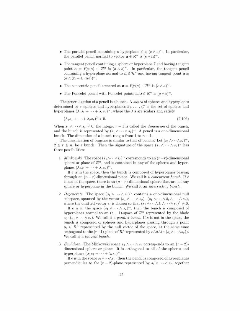
• The parallel pencil containing a hyperplane s is (e ∧ s)∼. In particular,the parallel pencil normal to vector n ∈ Rn is (e ∧ n)∼.

• The tangent pencil containing a sphere or hyperplane s and having tangentpoint a = P⊥

E (a) ∈ Rn is (a ∧ s)∼. In particular, the tangent pencilcontaining a hyperplane normal to n ∈ Rn and having tangent point a is(a ∧ (n + a · ne))∼.

• The concentric pencil centered at a = P⊥E (a) ∈ Rn is (e ∧ a)∼.

• The Poncelet pencil with Poncelet points a,b ∈ Rn is (a ∧ b)∼.

The generalization of a pencil is a bunch. A bunch of spheres and hyperplanesdetermined by r spheres and hyperplanes s1, . . . , s∼r is the set of spheres andhyperplanes (λ1s1 + · · · + λrsr)∼, where the λ’s are scalars and satisfy

(λ1s1 + · · · + λrsr)2 > 0. (2.106)

When s1 ∧ · · · ∧ sr �= 0, the integer r − 1 is called the dimension of the bunch,and the bunch is represented by (s1 ∧ · · · ∧ sr)∼. A pencil is a one-dimensionalbunch. The dimension of a bunch ranges from 1 to n − 1.

The classification of bunches is similar to that of pencils. Let (s1∧· · ·∧sr)∼,2 ≤ r ≤ n, be a bunch. Then the signature of the space (s1 ∧ · · · ∧ sr)∼ hasthree possibilities:

1. Minkowski. The space (s1∧· · ·∧sr)∼ corresponds to an (n−r)-dimensionalsphere or plane of Rn, and is contained in any of the spheres and hyper-planes (λ1s1 + · · · + λrsr)∼.

If e is in the space, then the bunch is composed of hyperplanes passingthrough an (n− r)-dimensional plane. We call it a concurrent bunch. If eis not in the space, there is an (n− r)-dimensional sphere that are on anysphere or hyperplane in the bunch. We call it an intersecting bunch.

2. Degenerate. The space (s1 ∧ · · · ∧ sr)∼ contains a one-dimensional nullsubspace, spanned by the vector (s1 ∧ · · · ∧ sr) · (s1 ∧ · · · ∧ si ∧ · · · ∧ sr),where the omitted vector si is chosen so that (s1 ∧ · · · ∧ si ∧ · · · ∧ sr)2 �= 0.

If e is in the space (s1 ∧ · · · ∧ sr)∼, then the bunch is composed ofhyperplanes normal to an (r − 1)-space of Rn represented by the bladee0 · (s1 ∧ · · · ∧ sr). We call it a parallel bunch. If e is not in the space, thebunch is composed of spheres and hyperplanes passing through a pointai ∈ Rn represented by the null vector of the space, at the same timeorthogonal to the (r−1)-plane of Rn represented by e∧a∧(e·(s1∧· · ·∧sr)).We call it a tangent bunch.

3. Euclidean. The Minkowski space s1 ∧ · · · ∧ sr corresponds to an (r − 2)-dimensional sphere or plane. It is orthogonal to all of the spheres andhyperplanes (λ1s1 + · · · + λrsr)∼.

If e is in the space s1∧· · ·∧sr, then the pencil is composed of hyperplanesperpendicular to the (r − 2)-plane represented by s1 ∧ · · · ∧ sr, together

25

Geometric conditions Bunch Ar Bunch Ar

Ar · A†r < 0 ,

e ∧ Ar = 0

Concurrent bunch,concurring at the(r − 2)-plane Ar

Concentric bunch,centered at the(r − 2)-plane Ar

Ar · A†r < 0 ,

e ∧ Ar �= 0

Intersecting bunch, atthe (r − 2)-sphere Ar

Poncelet bunch, withPoncelet sphere Ar

Ar · A†r = 0 ,

e ∧ Ar = 0

Parallel bunch, normalto the (n− r +1)-space(e0 · Ar)∼

Parallel bunch, normalto the (r − 1)-space

e ∧ e0 ∧ (e0 · Ar)

Ar · A†r = 0, e ∧ Ar �=

0, assuming a is a nullvector in the space Ar

Tangent bunch, atpoint a and orthogonalto the (n− r +1)-plane(e · Ar)∼

Tangent bunch, atpoint a and orthogonalto the (r − 1)-planee ∧ a ∧ (e · Ar)

Ar · A†r > 0 ,

e ∧ Ar = 0

Concentric bunch,centering at the(n − r)-plane Ar

Concurrent bunch,concurring at the(n − r)-plane Ar

Ar · A†r > 0 ,

e ∧ Ar �= 0

Poncelet bunch, withPoncelet sphere Ar

Intersecting bunch, atthe (n − r)-sphere Ar

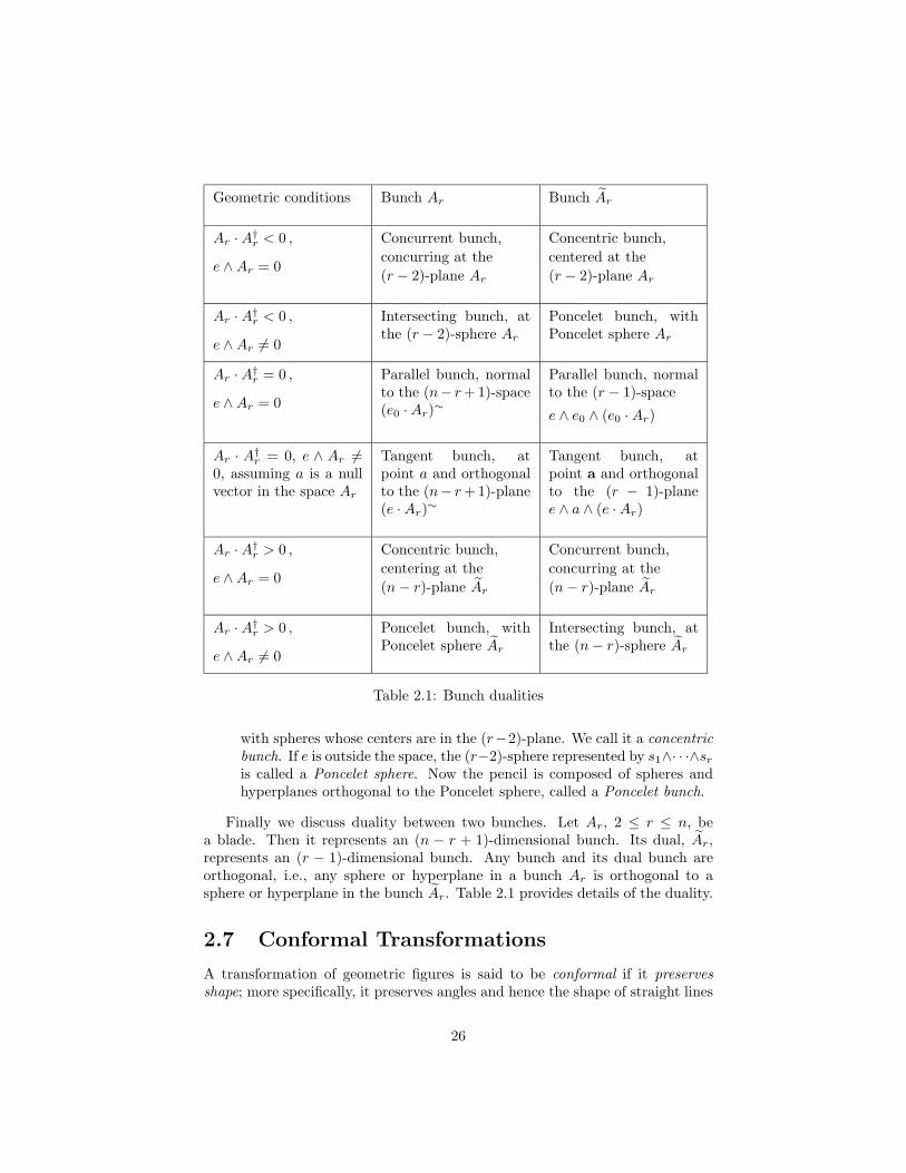
Table 2.1: Bunch dualities

with spheres whose centers are in the (r−2)-plane. We call it a concentricbunch. If e is outside the space, the (r−2)-sphere represented by s1∧· · ·∧sr

is called a Poncelet sphere. Now the pencil is composed of spheres andhyperplanes orthogonal to the Poncelet sphere, called a Poncelet bunch.

Finally we discuss duality between two bunches. Let Ar, 2 ≤ r ≤ n, bea blade. Then it represents an (n − r + 1)-dimensional bunch. Its dual, Ar,represents an (r − 1)-dimensional bunch. Any bunch and its dual bunch areorthogonal, i.e., any sphere or hyperplane in a bunch Ar is orthogonal to asphere or hyperplane in the bunch Ar. Table 2.1 provides details of the duality.

2.7 Conformal Transformations

A transformation of geometric figures is said to be conformal if it preservesshape; more specifically, it preserves angles and hence the shape of straight lines

26

and circles. As first proved by Liouville [L1850] for R3, any conformal trans-formation on the whole of Rn can be expressed as a composite of inversionsin spheres and reflections in hyperplanes. Here we show how the homogeneousmodel of En simplifies the formulation of this fact and thereby facilitates compu-tations with conformal transformations. Simplification stems from the fact thatthe conformal group on Rn is isomorphic to the Lorentz group on Rn+1. Hencenonlinear conformal transformations on Rn can be linearized by representingthem as Lorentz transformation and thereby further simplified as versor rep-resentations. The present treatment follows, with some improvements, [H91],where more details can be found.

From Chapter 1, we know that any Lorentz transformation G of a genericpoint x ∈ Rn+1 can be expressed in the form

G(x) = Gx(G∗)−1 = σx′ , (2.107)

where G is a versor and σ is a scalar. We are only interested in the action of Gon homogeneous points of En. Since the null cone is invariant under G, we have(x′)2 = x2 = 0. However, for fixed e, x · e is not Lorentz invariant, so a scalefactor σ has been introduced to ensure that x′ · e = x · e = −1 and x′ remains apoint in En. Expressing the right equality in (2.107) in terms of homogeneouspoints we have the expanded form

G[x + 12x

2e + e0 ](G∗)−1 = σ[x′ + 12 (x′)2e + e0 ] , (2.108)

where

x′ = g(x) (2.109)

is a conformal transformation on Rn and

σ = −e · (Gx) = −〈 eG∗xG−1 〉 . (2.110)

We study the simplest cases first.For reflection by a vector s = −s∗ (2.107) becomes

s(x) = −sxs−1 = x − 2(s · x)s−1 = σx′ , (2.111)

where sx + xs = 2s · x has been used. Both inversions and reflections have thisform as we now see by detailed examination.

Inversions. We have seen that a circle of radius ρ centered at point c =c + 1

2c2e + e0 is represented by the vector

s = c − 12ρ2e . (2.112)

We first examine the important special case of the unit sphere centered at theorigin in Rn. Then s reduces to e0 − 1

2e, so −2s · x = x2 − 1 and (2.111) gives

σx′ = (x+ 12x

2e+ e0)+ (x2 − 1)(e0 − 12e) = x2[x−1 + 1

2x−2e+ e0 ] .(2.113)

Whence the inversion

g(x) = x−1 =1x

=x

|x |2. (2.114)

27

Type g(x) on Rn Versor in Rn+1,1 σ(x)

Reflection −nxn + 2nδ s = n + eδ 1

Inversionρ2

x − c+ c s = c − 1

2ρ2e(x − c

ρ

)2

Rotation R(x − c)R−1 + c Rc = R+e(c×R) 1

Translation x − a Ta = 1 + 12ae 1

Transversionx − x2a

σ(x)Ka = 1 + ae0 1 − 2a · x + x2a2

Dilation λx Dλ = e−12 E ln λ λ−1

Involution x∗ = −x E = e ∧ e0 −1

Table 2.2: Conformal transformations and their versor representations (see textfor explanation)

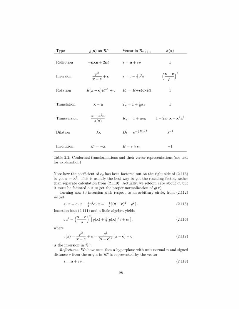
Note how the coefficient of e0 has been factored out on the right side of (2.113)to get σ = x2. This is usually the best way to get the rescaling factor, ratherthan separate calculation from (2.110). Actually, we seldom care about σ, butit must be factored out to get the proper normalization of g(x).

Turning now to inversion with respect to an arbitrary circle, from (2.112)we get

s · x = c · x − 12ρ2e · x = − 1

2 [ (x − c)2 − ρ2 ] . (2.115)

Insertion into (2.111) and a little algebra yields

σx′ =(x − c

ρ

)2[g(x) + 1

2 [g(x) ]2e + e0

], (2.116)

where

g(x) =ρ2

x − c+ c =

ρ2

(x − c)2(x − c) + c (2.117)

is the inversion in Rn.Reflections. We have seen that a hyperplane with unit normal n and signed

distance δ from the origin in Rn is represented by the vector

s = n + eδ . (2.118)

28

Inserting s · x = n · x − δ into (2.111) we easily find

g(x) = nxn∗ + 2nδ = n(x − nδ)n∗ + nδ . (2.119)

We recognize this as equivalent to a reflection nxn∗ at the origin translated byδ along the direction of n. A point c is on the hyperplane when δ = n · c, inwhich case (2.118) can be written

s = n + en · c . (2.120)

Via (2.119), this vector represents reflection in a hyperplane through point c.With a minor exception to be explained, all the basic conformal transforma-

tions in Table 2.2 can be generated from inversions and reflections. Let us seehow.

Translations. We have already seen in Chapter 1 that versor Ta in Table 2.2represents a translation. Now notice

(n + eδ)n = 1 + 12ae = Ta (2.121)

where a = 2δn. This tells us that the composite of reflections in two parallelhyperplanes is a translation through twice the distance between them.

Transversions. The transversion Ka in Table 2.2 can be generated from twoinversions and a translation; thus, using e0ee0 = −2e0 from (2.5c) and (2.5d),we find

e+Tae+ = (12e − e0)(1 + 1

2ae)( 12e − e0) = 1 + ae0 = Ka . (2.122)

The transversion generated by Ka can be put in the various forms

g(x) =x − x2a

1 − 2a · x + x2a2= x(1 − ax)−1 = (x−1 − a)−1 . (2.123)

The last form can be written down directly as an inversion followed by a trans-lation and another inversion as asserted by (2.122). That avoids a fairly messycomputation from (2.108).

Rotations. Using (2.120), the composition of reflections in two hyperplanesthrough a common point c is given by

(a + ea · c)(b + eb · c) = ab + ec · (a ∧ b) , (2.124)

where a and b are unit normals. Writing R = ab and noting that c · (a ∧ b) =c×R, we see that (2.124) is equivalent to the form for the rotation versor in Table2.2 that we found in Chapter 1. Thus we have established that the product oftwo reflections at any point is equivalent to a rotation about that point.

Dilations. Now we prove that the composite of two inversions centered atthe origin is a dilation (or dilatation). Using (2.5d) we have

(e0 − 12e)(e0 − 1

2ρ2e) = 12 (1 − E) + 1

2 (1 + E)ρ2 . (2.125)

Normalizing to unity and comparing to (2.6) with ρ = eϕ, we get

Dρ = 12 (1 + E)ρ + 1

2 (1 − E)ρ−1 = eEϕ , (2.126)

29

where Dρ is the square of the versor form for a dilation in Table 2.2. To verifythat Dρ does indeed generate a dilation, we note from (2.8) that

Dρ(e) = Dρ eD−1ρ = D2

ρ e = ρ−2e .

Similarly

Dρ(e0) = ρ2 e0 .

Therefore,

Dρ(x + 12x

2e + e0)D−1ρ = ρ2[ρ−2x + 1

2 (ρ−2x)2e + e0 ] . (2.127)

Thus g(x) = ρ−2x is a dilation as advertised.We have seen that every vector with positive signature in Rn+1,1 represents a

sphere or hyperplane as well as an inversion or reflection in same. They composea multiplicative group which we identify as the versor representation of the fullconformal group C(n) of En. Subject to a minor proviso explained below, ourconstruction shows that this conformal group is equivalent to the Lorentz groupof Rn+1,1. Products of an even number of these vectors constitute a subgroup,the spin group Spin+(n + 1, 1). It is known as the spin representation of theproper Lorentz group, the orthogonal group O+(n + 1, 1). This, in turn, isequivalent to the special orthogonal group SC+(n + 1, 1).

Our constructions above show that translations, transversions, rotations, di-lations belong to SC+(n). Moreover, every element of SC+(n) can be generatedfrom these types. This is easily proved by examining our construction of theirspin representations Ta, Kb, Rc, Dλ from products of vectors. One only needsto show that every other product of two vectors is equivalent to some product ofthese. Not hard! Comparing the structure of Ta, Kb, Rc, Dλ exhibited in Table2.2 with equations (2.6) through (2.15b), we see how it reflects the structure ofthe Minkowski plane R1,1 and groups derived therefrom.

Our construction of Spin+(n + 1, n) from products of vectors with posi-tive signature excludes the bivector E = e+e− because e2

− = −1. ExtendingSpin+(n + 1, n) by including E we get the full spin group Spin(n + 1, n). Un-like the elements of Spin+(n + 1, n), E is not parametrically connected to theidentity, so its inclusion gives us a double covering of Spin+(n + 1, n). Since Eis a versor, we can ascertain its geometric significance from (2.108); thus, using(2.5c) and (2.5a), we easily find

E(x + 12x

2e + e0)E = −[ − x + 12x

2e + e0 ] . (2.128)

This tells us that E represents the main involution x∗ = −x of Rn, as shown inTable 2.2. The conformal group can be extended to include involution, thoughthis is not often done. However, in even dimensions involution can be achievedby a rotation so the extension is redundant.

Including E in the versor group brings all vectors of negative signature alongwith it. For e− = Ee+ gives us one such vector, and Dλe− gives us (up to scalefactor) all the rest in the E-plane. Therefore, extension of the versor groupcorresponds only to extension of C(n) to include involution.

30

Since every versor G in Rn+1,1 can be generated as a product of vectors,expression of each vector in the expanded form (2.17) generates the expandedform

G = e(−e0A + B) − e0(C + eD) (2.129)

where A, B, C, D are versors in Rn and a minus sign is associated with e0 foralgebraic convenience in reference to (2.5d) and (2.2a). To enforce the versorproperty of G, the following conditions must be satisfied

AB†, BD†, CD†, AC† ∈ Rn , (2.130)

GG† = AD† − BC† = ±|G |2 �= 0 . (2.131)

Since G must have a definite parity, we can see from (2.129) that A and D musthave the same parity which must be opposite to the parity of C and D. This im-plies that the products in (2.130) must have odd parity. The stronger conditionthat these products must be vector-valued can be derived by generating G fromversor products or from the fact that the conformal transformation generatedby G must be vector-valued. For G ∈ Spin+(n + 1, n) the sign of (2.131) isalways positive, but for G ∈ Spin(n + 1, n) a negative sign may derive from avector of negative signature.

Adopting the normalization |G | = 1, we find

G∗† = ±(G∗)−1 = −(A∗†e0 + B∗†)e + (C∗† − D∗†e)e0 , (2.132)

and inserting the expanded form for G into (2.108), we obtain

g(x) = (Ax + B)(Cx + D)−1 (2.133)

with the rescaling factor

σ = σg(x) = (Cx + D)(C∗x + D∗)† . (2.134)

In evaluating (2.131) and (2.110) to get (2.134) it is most helpful to use theproperty 〈MN 〉 = 〈NM 〉 for the scalar part of any geometric product.

The general homeographic form (2.133) for a conformal transformation onRn is called a Mobius transformation by Ahlfors [A85]. Because of its nonlinearform it is awkward for composing transformations. However, composition can becarried out multiplicatively with the versor form (2.129) with the result insertedinto the homeographic form. As shown in [H91], the versor (2.133) has a 2 × 2matrix representation

[G

]=

[A BC D

], (2.135)

so composition can be carried out by matrix multiplication. Ahlfors [A86] hastraced this matrix representation back to Vahlen [V02].

The apparatus developed in this section is sufficient for efficient formulationand solution of any problem or theorem in conformal geometry. As an example,

31

consider the problem of deriving a conformal transformation on the whole ofRn from a given transformation of a finite set of points.

Let a1, · · · ,an+2 be distinct points in Rn spanning the whole space. Letb1, · · · ,bn+2 be another set of such points. If there is a Mobius transforma-tion g changing ai into bi for 1 ≤ i ≤ n + 2, then g must be induced by aLorentz transformation G of Rn+1,1, so the corresponding homogeneous pointsare related by

G(ai) = λibi, for 1 ≤ i ≤ n + 2 . (2.136)

Therefore ai · aj = (λibi) · (λjbj) and g exists if and only if the λ’s satisfy

(ai − aj)2 = λiλj(bi − bj)2 . for 1 ≤ i �= j ≤ n + 2, (2.137)

This sets (n + 2)(n − 1)/2 constraints on the b’s from which the λ’s can becomputed if they are satisfied.

Now assuming that g exists, we can employ (2.136) to compute g(x) for ageneric point x ∈ Rn. Using the ai as a basis, we write

x =n+1∑i=1

xiai, (2.138)

so G(x) =n+1∑i=1

xiλibi, and

g(x) =

n+1∑i=1

xiλibi

n+1∑i=1

xiλi

. (2.139)

The x’s can be computed by employing the basis dual to {ai} as explainedin Chapter 1.

If we are given, instead of n + 2 pairs of corresponding points, two setsof points, spheres and hyperplanes, say t1, · · · , tn+2, and u1, · · · , un+2, wheret2i ≥ 0 for 1 ≤ i ≤ n + 2 and where both sets are linearly independent vectorsin Rn+1,1, then we can simply replace the a’s with the t’s and the b’s with theu’s to compute g.

32

References

[A85] L. V. Ahlfors, Mobius transformations and Clifford numbers. In I.Chavel and H. M. Farkas, eds., Differential Geometry and ComplexAnalysis, Springer, Berlin, 1985.

[A86] L. V. Ahlfors, Mobius transformations in Rn expressed through2× 2 matrices of Clifford numbers,” Complex Variables Theory, 5:215–224 (1986).

[B53] L. M. Blumenthal, Theory and Applications of Distance Geome-try, Cambridge University Press, Cambridge, 1953; reprinted byChelsea, London, 1970.

[B61] L. M. Blumenthal, A Modern View of Geometry, Dover, New York,1961.

[DH93] A. Dress & T. Havel, Distance Geometry and Geometric Algebra,Foundations of Physics 23: 1357–1374, 1993.

[DHSA93] ∗C. Doran, D. Hestenes, F. Sommen, N. V. Acker, Lie groups asspin groups, J. Math. Phys. 34: 3642–3669, 1993.

[G1844] H. Grassmann, “Linear Extension Theory” (Die Lineale Ausdeh-nungslehre), translated by L. C. Kannenberg. In: The Aus-dehnungslehre of 1844 and Other Works (Chicago, La Salle: OpenCourt Publ. 1995).

[H98] T. Havel, Distance Geometry: Theory, Algorithms and Chemi-cal Applications. In: Encyclopedia of Computational Chemistry,J. Wiley & Sons (1998).

[H66] D. Hestenes, Space-Time Algebra, Gordon and Breach, New York,1966.

[H86] ∗ D. Hestenes, A unified language for mathematics and physics. In:Clifford Algebras and their Applications in Mathematical Physics,1–23, 1986 (J.S.R. Chisholm and A.K. Common, Eds.), KluwerAcademic Publishers, Dordrecht.

[H91] ∗D. Hestenes, The design of linear algebra and geometry, ActaAppl. Math. 23: 65–93, 1991.

[H94a] ∗D. Hestenes, Invariant body kinematics I: Saccadic and compen-satory eye movements, Neural Networks 7: 65–77, 1994.

[H94b] ∗D. Hestenes, Invariant body kinematics II: Reaching and neuroge-ometry, Neural Networks 7: 79–88, 1994.

33

[H96] ∗D. Hestenes, Grassmann’s Vision. In: Hermann Gunther Grass-mann (1809-1877): Visionary Mathematician, Scientist and Neo-humanist Scholar, 1996 (Gert Schubring, Ed.), Kluwer AcademicPublishers, Dordrecht.

[H98] D. Hestenes, New Foundations for Classical Mechanics, D. Reidel,Dordrecht/Boston, 2nd edition (1998).

[HS84] D. Hestenes and G. Sobczyk, Clifford Algebra to Geometric Calcu-lus, D. Reidel, Dordrecht/Boston, 1984.

[HZ91] ∗D. Hestenes and R. Ziegler, Projective Geometry with CliffordAlgebra, Acta Appl. Math. 23: 25–63, 1991.

[I92] B. Iversen, Hyperbolic Geometry, Cambridge, 1992.

[L97] H. Li, Hyperbolic Geometry with Clifford Algebra, Acta Appl.Math. 48: 317–358, 1997.

[L1850] J. Liouville, Extension au cas trois dimensions de la questiondu trace geographique. Applications de l’analyse a geometrie, G.Monge, Paris (1850), 609–616.

[M31] K. Menger, New foundation of Euclidean geometry, Am. J. Math.53: 721–745, 1931.

[S52] J. J. Seidel, Distance-geometric development of two-dimensionalEuclidean, hyperbolic and spherical geometry I, II, Simon Stevin29: 32–50, 5355–541, 1955; reprinted by Proc. Ned. Akad. Weten-sch.

[S55] J. J. Seidel, Angles and distance in n-dimensional Euclidean andnon-Euclidean geometry, I–III, Indag. Math. 17: 329–340, 65–76,1952.

[S88] P. Samuel, Projective Geometry, Springer Verlag, New York, 1988.

[S92] ∗G. Sobczyk, Simplicial Calculus with Geometric Algebra, In: Clif-ford Algebras and their Applications in Mathematical Physics (Eds:A. Micali et al), Kluwer Academic Publishers, Dordrecht/Boston,1992.

[V02] K. Vahlen, Uber Bewegungen und complexe Zahlen,Math. Ann. 55:585–593 (1902).

∗ Available at the Geometric Calculus Web Site:

<http://ModelingNTS.la.asu.edu/GC R&D.html>.

34