Hierarchical Bayesian Methods
Bhaskar D Rao1
University of California, San Diego
1Thanks to David Wipf, Jason Palmer, Zhilin Zhang, R. Prasad and RitwikGiri
Bhaskar D Rao University of California, San Diego

Bayesian Methods
1. MAP Estimation Framework (Type I)
2. Hierarchical Bayesian Framework (Type II)
Bhaskar D Rao University of California, San Diego

Bayesian Methods
1. MAP Estimation Framework (Type I)
2. Hierarchical Bayesian Framework (Type II)
Bhaskar D Rao University of California, San Diego

Bayesian Methods
1. MAP Estimation Framework (Type I)
2. Hierarchical Bayesian Framework (Type II)
Bhaskar D Rao University of California, San Diego

MAP Estimation Framework (Type I)
Problem Statement
x̂ = arg maxx
p(x |y) = arg maxx
p(y |x)p(x)
Choice of p(x) = a2e−a|x| as Laplacian and p(y |x) as Gaussian will lead
to the familiar LASSO framework.
Bhaskar D Rao University of California, San Diego

Hierarchical Bayes (Type II): Sparse BayesianLearning(SBL)
MAP methods were interested in the mode of the posterior p(x |y) butSBL uses posterior information beyond the mode, i.e. posteriordistribution p(x |y).
Problem
For all sparse priors it is not possible to compute the normalized posteriorp(x |y), hence some approximations are needed.
Bhaskar D Rao University of California, San Diego

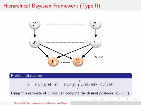
Hierarchical Bayesian Framework (Type II)
Problem Statement
γ̂ = arg maxγ
p(γ|y) = arg maxγ
∫p(y |x)p(x |γ)p(γ)dx
Using this estimate of γ, one can compute the desired posterior p(x |y ; γ̂).
Bhaskar D Rao University of California, San Diego
Hierarchical Bayesian Framework (Type II)
Problem Statement
γ̂ = arg maxγ
p(γ|y) = arg maxγ
∫p(y |x)p(x |γ)p(γ)dx
Using this estimate of γ, one can compute the desired posterior p(x |y ; γ̂).
Bhaskar D Rao University of California, San Diego

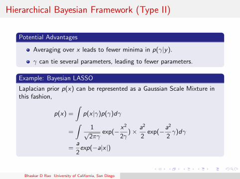
Hierarchical Bayesian Framework (Type II)
Potential Advantages
Averaging over x leads to fewer minima in p(γ|y).
γ can tie several parameters, leading to fewer parameters.
Example: Bayesian LASSO
Laplacian prior p(x) can be represented as a Gaussian Scale Mixture inthis fashion,
p(x) =
∫p(x |γ)p(γ)dγ
=
∫1√2πγ
exp(− x2
2γ)× a2
2exp(−a2
2γ)dγ
=a
2exp(−a|x |)
Bhaskar D Rao University of California, San Diego
Hierarchical Bayes: Sparse Bayesian Learning(SBL)
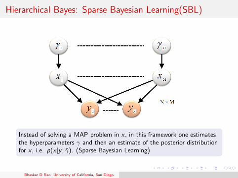
Instead of solving a MAP problem in x , in this framework one estimatesthe hyperparameters γ and then an estimate of the posterior distributionfor x , i.e. p(x |y ; γ̂). (Sparse Bayesian Learning)
Bhaskar D Rao University of California, San Diego

Hierarchical Bayes: Sparse Bayesian Learning(SBL)
Instead of solving a MAP problem in x , in this framework one estimatesthe hyperparameters γ and then an estimate of the posterior distributionfor x , i.e. p(x |y ; γ̂). (Sparse Bayesian Learning)
Bhaskar D Rao University of California, San Diego
Hierarchical Bayes: Sparse Bayesian Learning(SBL)
Instead of solving a MAP problem in x , in this framework one estimatesthe hyperparameters γ and then an estimate of the posterior distributionfor x , i.e. p(x |y ; γ̂). (Sparse Bayesian Learning)
Bhaskar D Rao University of California, San Diego

Useful Representation for Sparse priors
In order for this framework to be useful, we need tractablerepresentations:
Gaussian Scaled Mixtures (GSM)
Gaussian Scale Mixtures : Model for random variable X
X = γG where, G ∼ N(g ; 0, 1)
γ is a positive random variable, which is independent of G .
p(x) =
∫p(x |γ) p(γ)dγ
=
∫N(x ; 0, γ) p(γ)dγ
Bhaskar D Rao University of California, San Diego

Useful Representation for Sparse priors
In order for this framework to be useful, we need tractablerepresentations: Gaussian Scaled Mixtures (GSM)
Gaussian Scale Mixtures : Model for random variable X
X = γG where, G ∼ N(g ; 0, 1)
γ is a positive random variable, which is independent of G .
p(x) =
∫p(x |γ) p(γ)dγ
=
∫N(x ; 0, γ) p(γ)dγ
Bhaskar D Rao University of California, San Diego

Gaussian Scale Mixtures
Most of the sparse priors over x (including those with concave g) can berepresented in this GSM form, and different scale mixing density i.e, p(γi )will lead to different sparse priors. [Palmer et al., 2006]
Example: Laplacian density
p(x ; a) =a
2exp(−a|x |)
Scale mixing density: p(γ) = a2
2 exp(− a2
2 γ), γ ≥ 0.
Bhaskar D Rao University of California, San Diego
Examples of Gaussian Scale Mixtures
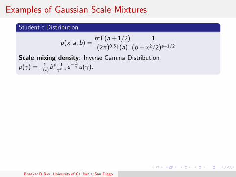
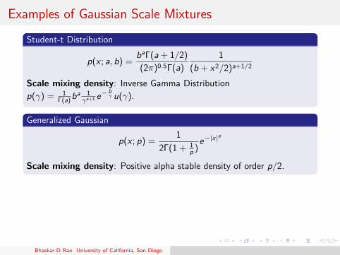
Student-t Distribution
p(x ; a, b) =baΓ(a + 1/2)
(2π)0.5Γ(a)
1
(b + x2/2)a+1/2
Scale mixing density: Inverse Gamma Distribution
p(γ) = 1Γ(a)b
a 1γa+1 e
− bγ u(γ).
Generalized Gaussian
p(x ; p) =1
2Γ(1 + 1p )
e−|x|p
Scale mixing density: Positive alpha stable density of order p/2.
Generalized logistic density
p(x ; a) =Γ(2α)
Γ(α)2
e−αx
(1 + e−x)2α
Scale mixing density: Related to Kolmogorov-Smirnov distancestatistics.
Bhaskar D Rao University of California, San Diego
Examples of Gaussian Scale Mixtures
Student-t Distribution
p(x ; a, b) =baΓ(a + 1/2)
(2π)0.5Γ(a)
1
(b + x2/2)a+1/2
Scale mixing density: Inverse Gamma Distribution
p(γ) = 1Γ(a)b
a 1γa+1 e
− bγ u(γ).
Generalized Gaussian
p(x ; p) =1
2Γ(1 + 1p )
e−|x|p
Scale mixing density: Positive alpha stable density of order p/2.
Generalized logistic density
p(x ; a) =Γ(2α)
Γ(α)2
e−αx
(1 + e−x)2α
Scale mixing density: Related to Kolmogorov-Smirnov distancestatistics.
Bhaskar D Rao University of California, San Diego

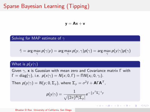
Sparse Bayesian Learning (Tipping)
y = Ax + v
Solving for MAP estimate of γ
γ̂ = arg maxγ
p(γ|y) = arg maxγ
p(y , γ)p(γ) = arg maxγ
p(y |γ)p(γ)
What is p(y |γ)
Given γ, x is Gaussian with mean zero and Covariance matrix Γ withΓ = diag(γ), i.e. p(x |γ) = N(x ; 0, Γ) = ΠN(xi ; 0, γi ).
Then p(y |γ) = N(y ; 0,Σy ), where Σy = σ2I + AΓAT ,
p(y |γ) =1√
(2π)N |Σy |e−
12 y
T Σ−1y y
Bhaskar D Rao University of California, San Diego

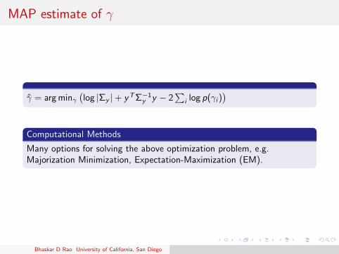
MAP estimate of γ
γ̂ = arg minγ(log |Σy |+ yTΣ−1
y y − 2∑
i log p(γi ))
Computational Methods
Many options for solving the above optimization problem, e.g.Majorization Minimization, Expectation-Maximization (EM).
Bhaskar D Rao University of California, San Diego
MAP estimate of γ
γ̂ = arg minγ(log |Σy |+ yTΣ−1
y y − 2∑
i log p(γi ))
Computational Methods
Many options for solving the above optimization problem, e.g.Majorization Minimization, Expectation-Maximization (EM).
Bhaskar D Rao University of California, San Diego

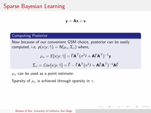
Sparse Bayesian Learning
y = Ax + v
Computing Posterior
Now because of our convenient GSM choice, posterior can be easilycomputed, i.e, p(x |y ; γ̂) = N(µx ,Σx) where,
µx = E [x |y ; γ̂] = Γ̂AT (σ2I + AΓ̂AT )−1y
Σx = Cov [x |y ; γ̂] = Γ̂− Γ̂AT (σ2I + AΓ̂AT )−1AΓ̂
µx can be used as a point estimate.
Sparsity of µx is achieved through sparsity in γ.
Another parameter of interest for the EM algorithm
E (x2i |y, γ̂) = µ2
x(i) + Σx(i , i)
Bhaskar D Rao University of California, San Diego

EM algorithm: Updating γ
Treating (y, x) as complete data and vector x as hidden variable.
log p(y , x , γ) = log p(y |x) + log p(x |γ) + log p(γ)
E step
Q(γ|γk) = Ex|y ;γk [log p(y |x) + log p(x |γ) + log p(γ)]
M step
γk+1 = argmaxγQ(γ|γk) = argmaxγEx|y ;γk [log p(x |γ) + log p(γ)]
= argminγEx|y ;γk [M∑i=1
(x2i
2γi+
1
2log γi
)− log p(γ)]
Solving this optimization problem with a non-informative prior p(γ),
γk+1i = E (x2
i |y, γk) = µx(i)2 + Σx(i , i)
Bhaskar D Rao University of California, San Diego

SBL properties
Local minima are sparse, i.e. have at most N nonzero γi
Cost function p(γ|y) is generally much smoother than theassociated MAP estimation objective p(x |y). Fewer local minima.
In high signal to noise ratio, the global minima is the sparsestsolution. No structural problems.
Attempts to approximate the posterior distribution p(x |y) in thearea with significant mass.
Bhaskar D Rao University of California, San Diego

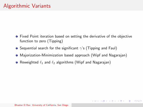
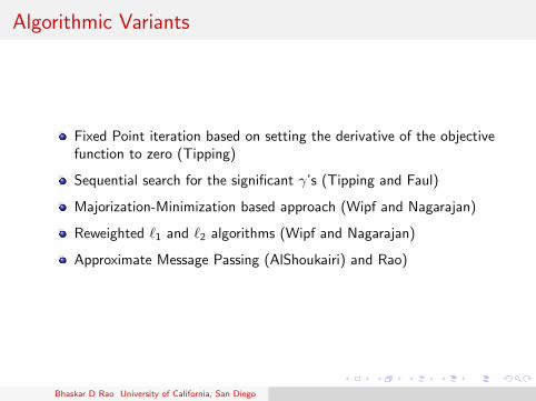
Algorithmic Variants
Fixed Point iteration based on setting the derivative of the objectivefunction to zero (Tipping)
Sequential search for the significant γ’s (Tipping and Faul)
Majorization-Minimization based approach (Wipf and Nagarajan)
Reweighted `1 and `2 algorithms (Wipf and Nagarajan)
Approximate Message Passing (AlShoukairi) and Rao)
Bhaskar D Rao University of California, San Diego

Empirical Comparison
For each test case
1 Generate a random dictionary A with 50 rows and 250 columnsfrom the normal distribution and normalize each column to have2-norm of 1.
2 Select the support for the true sparse coefficient vector x0 randomly.
3 Generate the non-zero components of x0 from the normaldistribution.
4 Compute signal, y = Ax0 (Noiseless case).
5 Compare SBL with previous methods with regard to estimating x0.
6 Average over 1000 independent trials.
Bhaskar D Rao University of California, San Diego

Empirical Comparison: 1000 trials
Figure: Probability of Successful recovery vs Number of non zerocoefficients
Bhaskar D Rao University of California, San Diego

Useful Extensions
Multiple Measurement Vectors (MMV)
Block Sparsity
Block MMV
MMV with time varying sparsity
Bhaskar D Rao University of California, San Diego

Useful Extensions
Multiple Measurement Vectors (MMV)
Block Sparsity
Block MMV
MMV with time varying sparsity
Bhaskar D Rao University of California, San Diego

Useful Extensions
Multiple Measurement Vectors (MMV)
Block Sparsity
Block MMV
MMV with time varying sparsity
Bhaskar D Rao University of California, San Diego

Useful Extensions
Multiple Measurement Vectors (MMV)
Block Sparsity
Block MMV
MMV with time varying sparsity
Bhaskar D Rao University of California, San Diego

Multiple Measurement Vectors (MMV)
Multiple measurements: L measurements
Common Sparsity Profile: k nonzero rows
Bhaskar D Rao University of California, San Diego

Multiple Measurement Vectors (MMV)
Multiple measurements: L measurements
Common Sparsity Profile: k nonzero rows
Bhaskar D Rao University of California, San Diego

Multiple Measurement Vectors (MMV)
Multiple measurements: L measurements
Common Sparsity Profile: k nonzero rows
Bhaskar D Rao University of California, San Diego

Block Sparsity
Variations include equal blocks, unequal blocks, block boundary known orunknown.
Bhaskar D Rao University of California, San Diego

Block Sparsity
Variations include equal blocks, unequal blocks, block boundary known orunknown.
Bhaskar D Rao University of California, San Diego

Block Sparsity
Variations include equal blocks, unequal blocks, block boundary known orunknown.
Bhaskar D Rao University of California, San Diego

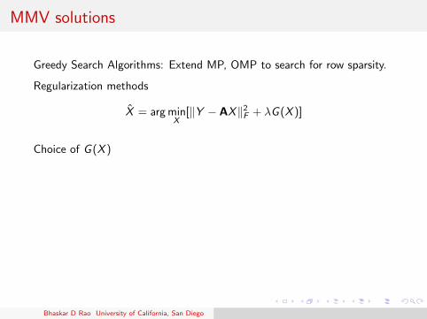
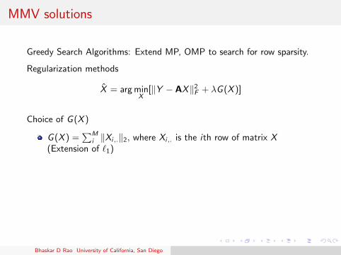
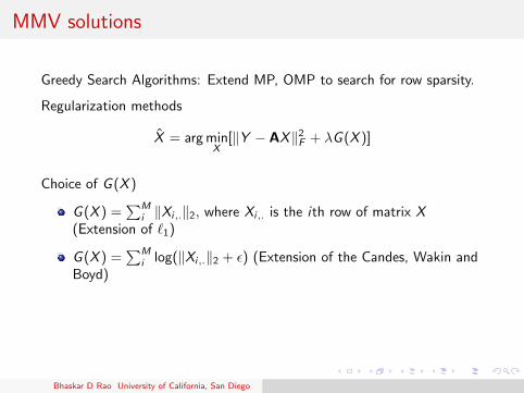
MMV solutions
Greedy Search Algorithms: Extend MP, OMP to search for row sparsity.
Regularization methods
X̂ = arg minX
[‖Y − AX‖2F + λG (X )]
Choice of G (X )
G (X ) =∑M
i ‖Xi,.‖2, where Xi,. is the ith row of matrix X(Extension of `1)
G (X ) =∑M
i log(‖Xi,.‖2 + ε) (Extension of the Candes, Wakin andBoyd)
G (X ) =∑M
i log(‖Xi,.‖22 + ε) (Extension of the Chartrand and Yin
penalty)
Bhaskar D Rao University of California, San Diego

MMV solutions
Greedy Search Algorithms:
Extend MP, OMP to search for row sparsity.
Regularization methods
X̂ = arg minX
[‖Y − AX‖2F + λG (X )]
Choice of G (X )
G (X ) =∑M
i ‖Xi,.‖2, where Xi,. is the ith row of matrix X(Extension of `1)
G (X ) =∑M
i log(‖Xi,.‖2 + ε) (Extension of the Candes, Wakin andBoyd)
G (X ) =∑M
i log(‖Xi,.‖22 + ε) (Extension of the Chartrand and Yin
penalty)
Bhaskar D Rao University of California, San Diego

MMV solutions
Greedy Search Algorithms: Extend MP, OMP to search for row sparsity.
Regularization methods
X̂ = arg minX
[‖Y − AX‖2F + λG (X )]
Choice of G (X )
G (X ) =∑M
i ‖Xi,.‖2, where Xi,. is the ith row of matrix X(Extension of `1)
G (X ) =∑M
i log(‖Xi,.‖2 + ε) (Extension of the Candes, Wakin andBoyd)
G (X ) =∑M
i log(‖Xi,.‖22 + ε) (Extension of the Chartrand and Yin
penalty)
Bhaskar D Rao University of California, San Diego

MMV solutions
Greedy Search Algorithms: Extend MP, OMP to search for row sparsity.
Regularization methods
X̂ = arg minX
[‖Y − AX‖2F + λG (X )]
Choice of G (X )
G (X ) =∑M
i ‖Xi,.‖2, where Xi,. is the ith row of matrix X(Extension of `1)
G (X ) =∑M
i log(‖Xi,.‖2 + ε) (Extension of the Candes, Wakin andBoyd)
G (X ) =∑M
i log(‖Xi,.‖22 + ε) (Extension of the Chartrand and Yin
penalty)
Bhaskar D Rao University of California, San Diego

Bayesian Methods
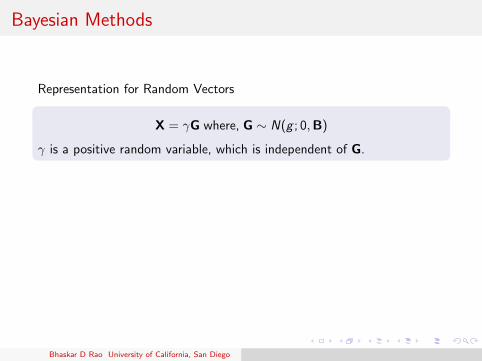
Representation for Random Vectors
X = γG where, G ∼ N(g ; 0,B)
γ is a positive random variable, which is independent of G.
p(x) =
∫p(x|γ) p(γ)dγ
=
∫N(x; 0, γB) p(γ)dγ
B = I if the row entries are assumed independent.
Bhaskar D Rao University of California, San Diego
Bayesian Methods
Representation for Random Vectors
X = γG where, G ∼ N(g ; 0,B)
γ is a positive random variable, which is independent of G.
p(x) =
∫p(x|γ) p(γ)dγ
=
∫N(x; 0, γB) p(γ)dγ
B = I if the row entries are assumed independent.
Bhaskar D Rao University of California, San Diego

Bayesian Methods
Representation for Random Vectors
X = γG where, G ∼ N(g ; 0,B)
γ is a positive random variable, which is independent of G.
p(x) =
∫p(x|γ) p(γ)dγ
=
∫N(x; 0, γB) p(γ)dγ
B = I if the row entries are assumed independent.
Bhaskar D Rao University of California, San Diego

Bayesian Methods
Representation for Random Vectors
X = γG where, G ∼ N(g ; 0,B)
γ is a positive random variable, which is independent of G.
p(x) =
∫p(x|γ) p(γ)dγ
=
∫N(x; 0, γB) p(γ)dγ
B = I if the row entries are assumed independent.
Bhaskar D Rao University of California, San Diego

EM algorithm: Updating γ
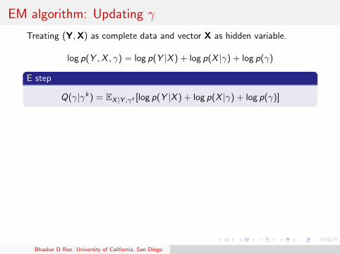
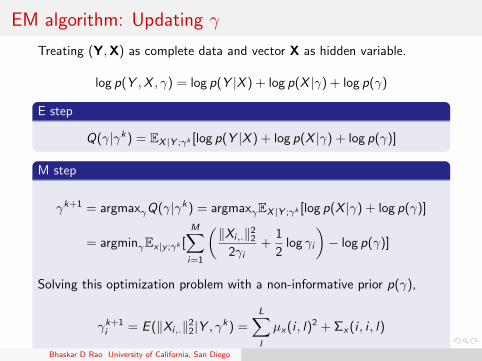
Treating (Y,X) as complete data and vector X as hidden variable.
log p(Y ,X , γ) = log p(Y |X ) + log p(X |γ) + log p(γ)
E step
Q(γ|γk) = EX |Y ;γk [log p(Y |X ) + log p(X |γ) + log p(γ)]
M step
γk+1 = argmaxγQ(γ|γk) = argmaxγEX |Y ;γk [log p(X |γ) + log p(γ)]
= argminγEx|y ;γk [M∑i=1
(‖Xi,.‖2
2
2γi+
1
2log γi
)− log p(γ)]
Solving this optimization problem with a non-informative prior p(γ),
γk+1i = E (‖Xi,.‖2
2|Y , γk) =L∑l
µx(i , l)2 + Σx(i , i , l)
Bhaskar D Rao University of California, San Diego

EM algorithm: Updating γ
Treating (Y,X) as complete data and vector X as hidden variable.
log p(Y ,X , γ) = log p(Y |X ) + log p(X |γ) + log p(γ)
E step
Q(γ|γk) = EX |Y ;γk [log p(Y |X ) + log p(X |γ) + log p(γ)]
M step
γk+1 = argmaxγQ(γ|γk) = argmaxγEX |Y ;γk [log p(X |γ) + log p(γ)]
= argminγEx|y ;γk [M∑i=1
(‖Xi,.‖2
2
2γi+
1
2log γi
)− log p(γ)]
Solving this optimization problem with a non-informative prior p(γ),
γk+1i = E (‖Xi,.‖2
2|Y , γk) =L∑l
µx(i , l)2 + Σx(i , i , l)
Bhaskar D Rao University of California, San Diego

Empirical Comparison: Multiple Measurement Vectors(MMV)
Generate data matrix via Y = ΦX0 (noiseless), where:
1 X0 is 100-by-5 with random non-zero rows.
2 Φ is 50-by-100 with Gaussian iid entries.
Bhaskar D Rao University of California, San Diego

MMV Empirical Comparison: 1000 trials
Bhaskar D Rao University of California, San Diego

Summary
Sparse Signal Recovery (SSR) and Compressed Sensing (CS) areinteresting new signal processing tools with many potentialapplications.
Many algorithmic options exist to solve the underlying sparse signalrecovery problem; Greedy Search Techniques, regularizationmethods, Bayesian methods, among others
Nice theoretical results particularly for the greedy search algorithmsand `1 recovery methods.
Bayesian methods offer interesting algorithmic options to the SparseSignal Recovery problem
MAP methods (reweighted `1 and `2 methods)Hierarchical Bayesian Methods (Sparse Bayesian Learning)Versatile and can be more easily employed in problems withstructureAlgorithms can often be justified by studying the resultingobjective functions.
More applications to come enriching the field.
Bhaskar D Rao University of California, San Diego

Summary
Sparse Signal Recovery (SSR) and Compressed Sensing (CS) areinteresting new signal processing tools with many potentialapplications.
Many algorithmic options exist to solve the underlying sparse signalrecovery problem; Greedy Search Techniques, regularizationmethods, Bayesian methods, among others
Nice theoretical results particularly for the greedy search algorithmsand `1 recovery methods.
Bayesian methods offer interesting algorithmic options to the SparseSignal Recovery problem
MAP methods (reweighted `1 and `2 methods)
Hierarchical Bayesian Methods (Sparse Bayesian Learning)Versatile and can be more easily employed in problems withstructureAlgorithms can often be justified by studying the resultingobjective functions.
More applications to come enriching the field.
Bhaskar D Rao University of California, San Diego

Summary
Sparse Signal Recovery (SSR) and Compressed Sensing (CS) areinteresting new signal processing tools with many potentialapplications.
Many algorithmic options exist to solve the underlying sparse signalrecovery problem; Greedy Search Techniques, regularizationmethods, Bayesian methods, among others
Nice theoretical results particularly for the greedy search algorithmsand `1 recovery methods.
Bayesian methods offer interesting algorithmic options to the SparseSignal Recovery problem
MAP methods (reweighted `1 and `2 methods)Hierarchical Bayesian Methods (Sparse Bayesian Learning)
Versatile and can be more easily employed in problems withstructureAlgorithms can often be justified by studying the resultingobjective functions.
More applications to come enriching the field.
Bhaskar D Rao University of California, San Diego

Summary
Sparse Signal Recovery (SSR) and Compressed Sensing (CS) areinteresting new signal processing tools with many potentialapplications.
Many algorithmic options exist to solve the underlying sparse signalrecovery problem; Greedy Search Techniques, regularizationmethods, Bayesian methods, among others
Nice theoretical results particularly for the greedy search algorithmsand `1 recovery methods.
Bayesian methods offer interesting algorithmic options to the SparseSignal Recovery problem
MAP methods (reweighted `1 and `2 methods)Hierarchical Bayesian Methods (Sparse Bayesian Learning)Versatile and can be more easily employed in problems withstructure
Algorithms can often be justified by studying the resultingobjective functions.
More applications to come enriching the field.
Bhaskar D Rao University of California, San Diego

Summary
Sparse Signal Recovery (SSR) and Compressed Sensing (CS) areinteresting new signal processing tools with many potentialapplications.
Many algorithmic options exist to solve the underlying sparse signalrecovery problem; Greedy Search Techniques, regularizationmethods, Bayesian methods, among others
Nice theoretical results particularly for the greedy search algorithmsand `1 recovery methods.
Bayesian methods offer interesting algorithmic options to the SparseSignal Recovery problem
MAP methods (reweighted `1 and `2 methods)Hierarchical Bayesian Methods (Sparse Bayesian Learning)Versatile and can be more easily employed in problems withstructureAlgorithms can often be justified by studying the resultingobjective functions.
More applications to come enriching the field.
Bhaskar D Rao University of California, San Diego

Summary
Sparse Signal Recovery (SSR) and Compressed Sensing (CS) areinteresting new signal processing tools with many potentialapplications.
Many algorithmic options exist to solve the underlying sparse signalrecovery problem; Greedy Search Techniques, regularizationmethods, Bayesian methods, among others
Nice theoretical results particularly for the greedy search algorithmsand `1 recovery methods.
Bayesian methods offer interesting algorithmic options to the SparseSignal Recovery problem
MAP methods (reweighted `1 and `2 methods)Hierarchical Bayesian Methods (Sparse Bayesian Learning)Versatile and can be more easily employed in problems withstructureAlgorithms can often be justified by studying the resultingobjective functions.
More applications to come enriching the field.Bhaskar D Rao University of California, San Diego
Recommended