Hierarchical Graphical Bayesian Models in Psychology · Hierarchical Graphical Bayesian Models in Psychology 321 isaprobabilitythatananimalbelongstoacategoryofanimal(e.g.,mammal),a

Revista Colombiana de EstadísticaCurrent Topics in Statistical Graphics

Diciembre 2014, volumen 37, no. 2, pp. 319 a 339DOI: http://dx.doi.org/10.15446/rce.v37n2spe.47940

Hierarchical Graphical Bayesian Models inPsychology

Modelos Bayesianos gráficos jerárquicos en psicología

Guillermo Campitelli1,a, Guillermo Macbeth2,b

1School of Psychology and Social Science, Edith Cowan University, MountLawley, Australia

2Facultad de Ciencias de la Educación, Universidad Nacional de Entre Ríos,Argentina

AbstractThe improvement of graphical methods in psychological research can pro-

mote their use and a better comprehension of their expressive power. Theapplication of hierarchical Bayesian graphical models has recently becomemore frequent in psychological research. The aim of this contribution is tointroduce suggestions for the improvement of hierarchical Bayesian graphicalmodels in psychology. This novel set of suggestions stems from the descrip-tion and comparison between two main approaches concerned with the use ofplate notation and distribution pictograms. It is concluded that the combi-nation of relevant aspects of both models might improve the use of powerfulhierarchical Bayesian graphical models in psychology.

Key words: Visual Statistics, Graphical Models, Bayesian Statistics, Hier-archical Models, Psychology, Statistical Cognition.

ResumenEl mejoramiento de los métodos gráficos en la investigación en psicología

puede promover su uso y una mejor compresión de su poder de expresión.La aplicación de modelos Bayesianos gráficos jerárquicos se ha vuelto másfrecuente en la investigación en psicología. El objetivo de este trabajo esintroducir sugerencias para el mejoramiento de los modelos Bayesianos grá-ficos jerárquicos en psicología. Este conjunto de sugerencias se apoya enla descripción y comparación entre los dos enfoques principales con el usode notación y pictogramas de distribución. Se concluye que la combinaciónde los aspectos relevantes de ambos puede mejorar el uso de los modelosBayesianos gráficos jerárquicos en psicología

Palabras clave: cognición estadística, estadística Bayesiana, estadística vi-sual, modelos gráficos, modelos jerárquicos, psicología.

aLecturer. E-mail: [email protected]. E-mail: [email protected]

319

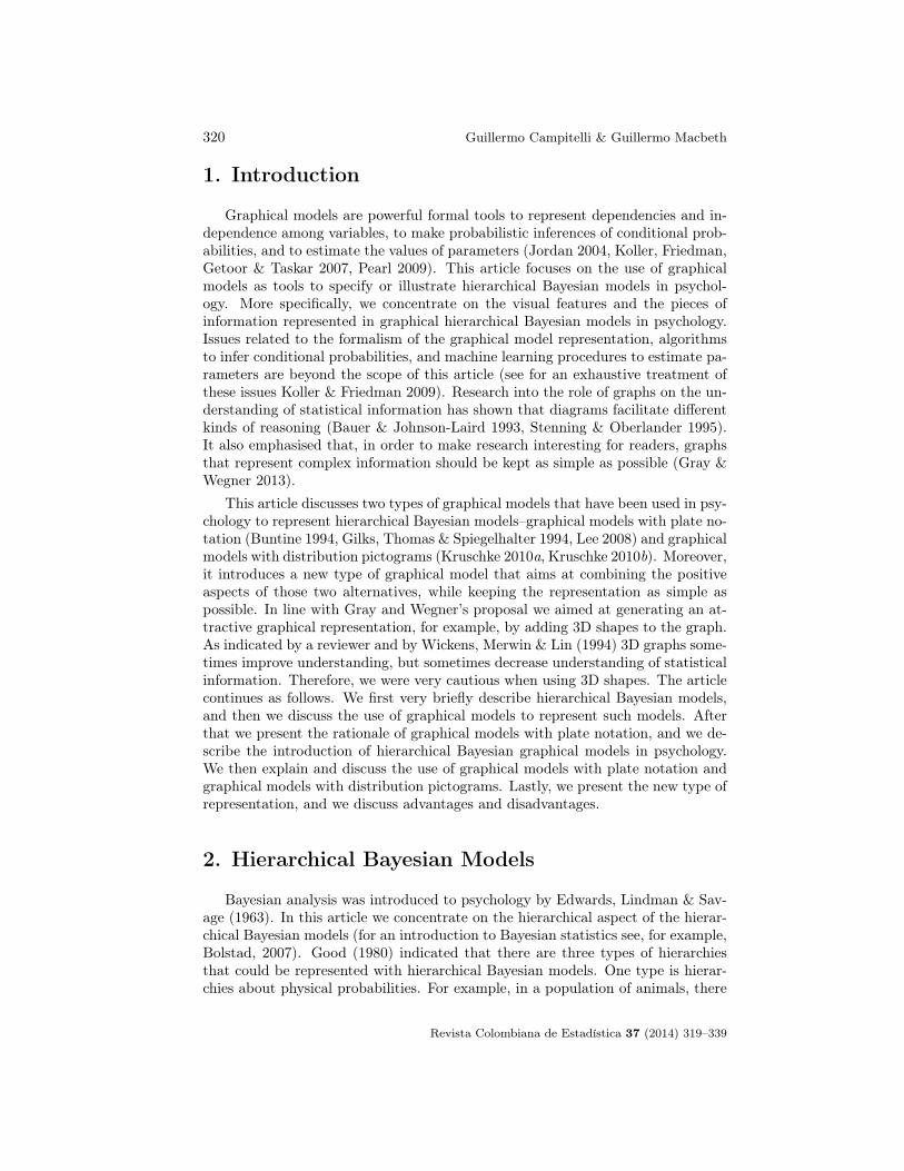
320 Guillermo Campitelli & Guillermo Macbeth

1. Introduction

Graphical models are powerful formal tools to represent dependencies and in-dependence among variables, to make probabilistic inferences of conditional prob-abilities, and to estimate the values of parameters (Jordan 2004, Koller, Friedman,Getoor & Taskar 2007, Pearl 2009). This article focuses on the use of graphicalmodels as tools to specify or illustrate hierarchical Bayesian models in psychol-ogy. More specifically, we concentrate on the visual features and the pieces ofinformation represented in graphical hierarchical Bayesian models in psychology.Issues related to the formalism of the graphical model representation, algorithmsto infer conditional probabilities, and machine learning procedures to estimate pa-rameters are beyond the scope of this article (see for an exhaustive treatment ofthese issues Koller & Friedman 2009). Research into the role of graphs on the un-derstanding of statistical information has shown that diagrams facilitate differentkinds of reasoning (Bauer & Johnson-Laird 1993, Stenning & Oberlander 1995).It also emphasised that, in order to make research interesting for readers, graphsthat represent complex information should be kept as simple as possible (Gray &Wegner 2013).

This article discusses two types of graphical models that have been used in psy-chology to represent hierarchical Bayesian models–graphical models with plate no-tation (Buntine 1994, Gilks, Thomas & Spiegelhalter 1994, Lee 2008) and graphicalmodels with distribution pictograms (Kruschke 2010a, Kruschke 2010b). Moreover,it introduces a new type of graphical model that aims at combining the positiveaspects of those two alternatives, while keeping the representation as simple aspossible. In line with Gray and Wegner’s proposal we aimed at generating an at-tractive graphical representation, for example, by adding 3D shapes to the graph.As indicated by a reviewer and by Wickens, Merwin & Lin (1994) 3D graphs some-times improve understanding, but sometimes decrease understanding of statisticalinformation. Therefore, we were very cautious when using 3D shapes. The articlecontinues as follows. We first very briefly describe hierarchical Bayesian models,and then we discuss the use of graphical models to represent such models. Afterthat we present the rationale of graphical models with plate notation, and we de-scribe the introduction of hierarchical Bayesian graphical models in psychology.We then explain and discuss the use of graphical models with plate notation andgraphical models with distribution pictograms. Lastly, we present the new type ofrepresentation, and we discuss advantages and disadvantages.

2. Hierarchical Bayesian Models

Bayesian analysis was introduced to psychology by Edwards, Lindman & Sav-age (1963). In this article we concentrate on the hierarchical aspect of the hierar-chical Bayesian models (for an introduction to Bayesian statistics see, for example,Bolstad, 2007). Good (1980) indicated that there are three types of hierarchiesthat could be represented with hierarchical Bayesian models. One type is hierar-chies about physical probabilities. For example, in a population of animals, there

Revista Colombiana de Estadística 37 (2014) 319–339

Hierarchical Graphical Bayesian Models in Psychology 321

is a probability that an animal belongs to a category of animal (e.g., mammal), aprobability that it belongs to a species (e.g., dog), a probability that belongs toan age category (e.g., 1 year of age), and so forth.

The second type of hierarchy arises from the fact that subjective probabilitiesabout events cannot be sharp (e.g., the probability of an article being acceptedbeing 0.65474). One way of dealing with this is to express the confidence of thissubjective probability, and represent it as a probability distribution of a highertype. The third type of hierarchy is a combination of the first two types. Lee(2008) takes a pragmatic approach, and considers that a Bayesian model is hierar-chical when it is more complex than a Bayesian model with a set of parameters θgenerating a set of data d through a likelihood function f(.). Similarly, Kruschke’s(2010a) chapter on hierarchical Bayesian models includes hyper-parameters, whichare parameters that do not generate data, instead they affect other parameters.

3. Graphical Model Representation of HierarchicalBayesian Models

Jordan (2004) indicated that a graphical model is a family of probability dis-tributions represented in a directed or undirected graph. Graphs contain nodes–which represent random variables– connected by edges, which could be either di-rected (i.e., arrows) or undirected (i.e., lines). The most popular graphical modelsare Markov networks and Bayesian networks (or “Bayes nets”). In Markov net-works all the edges are undirected whereas in the Bayesian networks all the edgesare directed and the graph is acyclic. A graph is cyclic if it contains a cyclic path.A path is a sequence of nodes in which each node, except the first node in thesequence, receives a directed edge from the precedent node in the sequence (e.g.,o→ o→ o→ o). When the last node in the sequence is the same as the first node,the path is cyclic, otherwise it is acyclic. In this article we focus on directed acyclicgraphs (DAG). Although graphical models could be used both by frequentist andBayesian approaches, they are very powerful tools to formulate complex modelsof joint probability distributions; hence, they have been very popular within theBayesian approach (Jordan 2004). We present more details of graphical models inthe following sections.

4. Plate Notation in Graphical ModelRepresentations of Hierarchical Bayesian Models

The plate notation was introduced by Buntine (1994)1 in order to solve theproblem that graphical models were not representing the fact that the learningalgorithms to estimate parameters had to do so over a repeated set of measured

1Note that Buntine indicated that the notion of plate was personally communicated to himby Spiegelhalter in 1993, but the similar notion of “replicated node” was developed by himindependently, and that in order to maintain the same language he used the term plate.



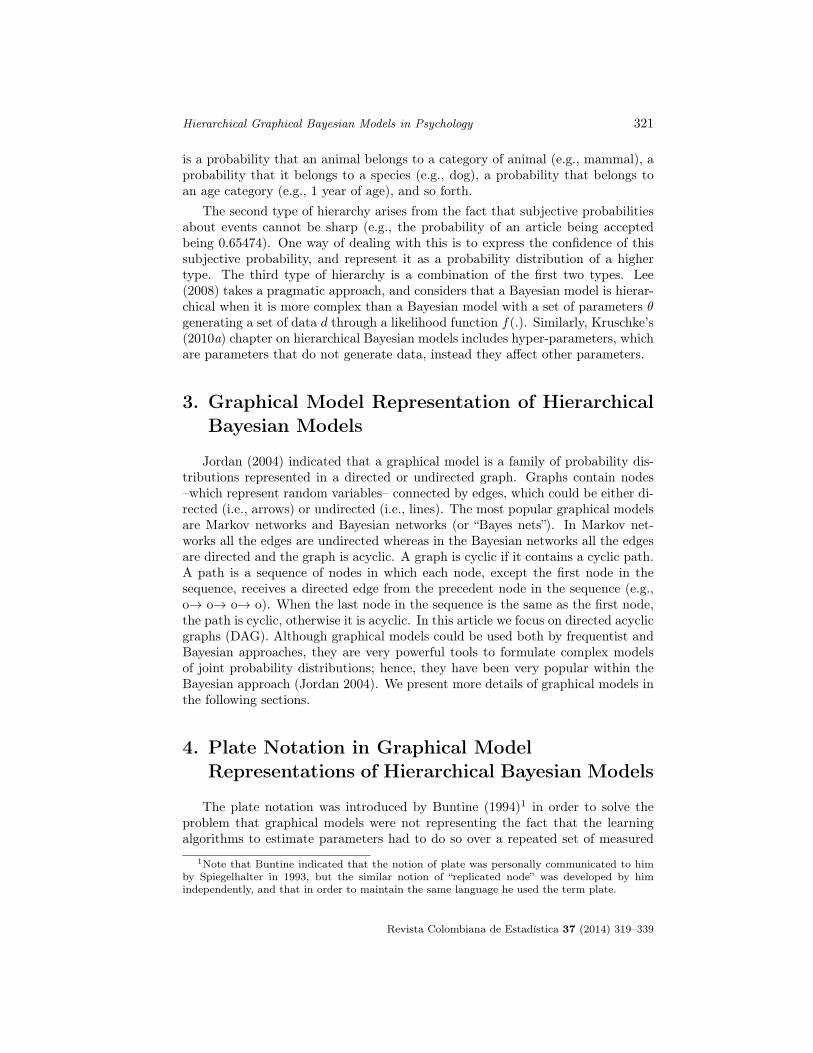
variables. Figure 1 is an adaptation of Buntine’s Figure 13, which shows howrepetition of variables were represented without plates (panel a) and the samemodel represented with plates (panel b). The graphical model represents a biasedcoin toss experiment in which the probability of heads is θ , and the coin is tossedN times. Each time the coin is tossed the experimenter records whether it was ahead or not. The hierarchical aspect of the model is apparent by the introductionof a prior distribution in the graph–that is, a Beta distribution with parametersa = 1.5 and b = 1.5–from which the parameter θ is generated.

a) b)

heads 1

heads 2

heads N

. . . Beta (1.5, 1.5)

θ heads 1

N Beta (1.5, 1.5)

θ

Figure 1: Adaptation of the plate graphical model (in panel b) presented by Buntine(1994) to represent the graphical model without plates in panel a. Insteadof representing a number of nodes of the variable heads as in panel a, theplate representation surrounds one heads node by a plate, indicating thatthe model structure is repeated N times. Shaded nodes indicate observedvariables and unshaded nodes indicate unobserved variables. The arrowsshow the dependencies between the variables.

There is nothing wrong with the model without plates, but when the numberof variables and parameters increases the graphical model becomes difficult to rep-resent in a limited space. The plate indicates that the variables within that plateare repeated the number of times indicated in the plate (in the model presented inFigure 1b, N times). This version of plate notation includes other important fea-tures: shaded nodes indicate observed data or variables with known values whereasunshaded nodes are unobserved variables. In other graphical models in the articleBuntine (1994) used a double border to represent deterministic variables (the samenotation was adopted by Lee (2008); see Figure 5.1, variables hi and fi). A noteof interest is that Buntine included in the graph the Beta distribution from whichthe parameter θ is generated, but not the Bernoulli distribution by which eachvalue in heads is obtained.

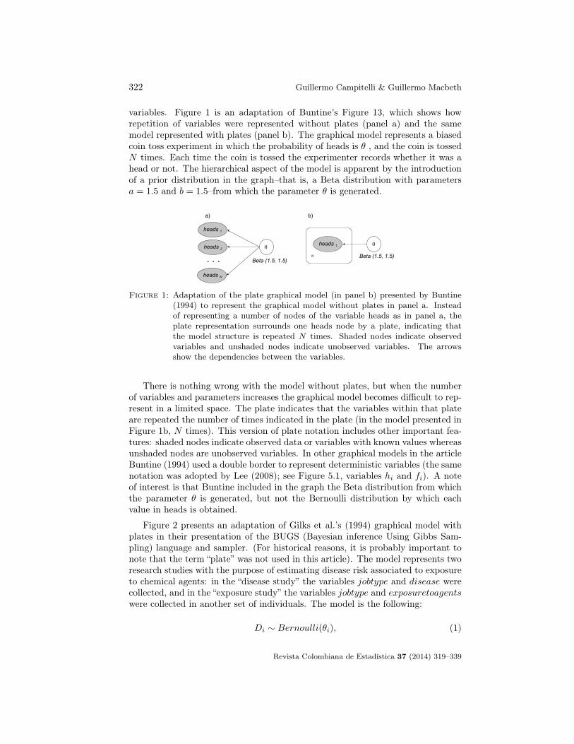
Figure 2 presents an adaptation of Gilks et al.’s (1994) graphical model withplates in their presentation of the BUGS (Bayesian inference Using Gibbs Sam-pling) language and sampler. (For historical reasons, it is probably important tonote that the term “plate” was not used in this article). The model represents tworesearch studies with the purpose of estimating disease risk associated to exposureto chemical agents: in the “disease study” the variables jobtype and disease werecollected, and in the “exposure study” the variables jobtype and exposuretoagentswere collected in another set of individuals. The model is the following:

Di ∼ Bernoulli(θi), (1)



Figure 2: Graphical model with plates presented by Gilks et al. (1994). Circle nodesdenote unobserved stochastic variables, square nodes with a single border rep-resent observed stochastic variables (i.e., data), squares with double borderdenote fixed quantities in prior distributions, and triangles denote determin-istic variables. The arrows represent the dependencies between variables. Inthis model all the arrows represent stochastic dependencies.

where Di is the disease status of the ith individual and θi is his/her probability ofdisease

logit(θi) = β0 +

nA∑k=1

βkEik, (2)

where Eik is the unobserved exposure status (0 = unexposed; 1 = exposed) ofthe ith individual to the kth chemical agent, and nA = 4 is the number of chemicalagents. The model for the exposure study is:

mjk ∼ Binomial(πjk, nj), (3)

where j = 1 to nJ , nJ = 2 is the number of job types, πjk is an exposureprobability, nj is the number of individuals in the exposure study who were in jobtype j, and mjk is the number of those individuals in job type j who were exposedto chemical agent k. The connection between the disease study and the exposurestudy is indicated by:

Eik ∼ Bernoulli(πj(i)k), (4)

where j(i) is the job type of individual i in the “disease study”. The priors aredenoted by:

βk ∼ Normal(µk, σ2k) (5)

and

logit(πjk) = φjk, (6)

withφjk ∼ Normal(µ∗k, σ∗2k ) (7)



The graphical representation of this Bayesian hierarchical model in Figure 2contains the plates i, j, k. The variables within each plate are replicated for eachunit indicated in the plate. For example, Di indicates that there is a value ofdisease for each individual i, and nj that there is a value for the variable n foreach job type j (e.g., 10 individuals are drivers, 25 individuals are teachers, etc.).The number of replications of variables that are contained in two plates (e.g., iand j ) is the product of the number of units indicated in each plate (e.g., numberof i units x number of k units). The replication aspect of this graphical model isidentical to that of Buntine (1994).

However, there are a number of differences in the graphical representations. InGilks et al. (1994) there are no shaded nodes, and the difference between observedand unobserved variables is given by the shape of the nodes. Circles denote un-observed stochastic variables, square nodes with a single border denote observedstochastic variables (i.e., data), squares with double border denote fixed quantitiesin prior distributions, and triangles denote deterministic variables. Another differ-ence is that in Gilks et al. (1994) the name of the distributions are not included,and instead of including the total number of units per plate they present the unitindex (i.e., i, j, k), the name of the units (i.e., individuals, jobs, agents), and theindices of the variables are located within the nodes.

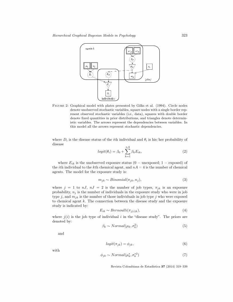
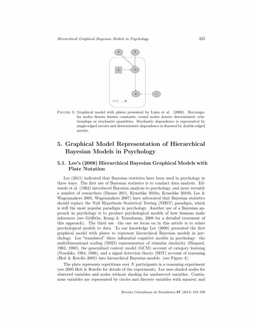
Lunn, Thomas, Best & Spiegelhalter (2000) presented WinBUGS, which usesa graphical interface called DoodleBUGS. The graphical representation code inDoodleBUGS differs from the previous two versions. Figure 3 shows the simpleexample presented by Lunn et al. (2000), in which the graphical model representsa linear regression model expressed by

yi ∼ N(µi, τ−1), (8)

where yi are observations measured at an experiment design points’ xi, i =1, . . . , N, τ is the inverse of the residual variance, and

µi = α+ βxi, (9)

for i = 1, . . . , N . α is the intercept parameter, β is the slope parameter, and bothare unknown.

In this representation rectangular nodes denote known constants, and roundnodes denote deterministic relationships or stochastic quantities. Stochastic de-pendence is represented by single-edged arrows and deterministic dependence isdenoted by double-edged arrows. The plate includes both the index of the units(i.e., i) and the fact that the repetition is from i unit 1 to i unit N .

Summing up, a number of visual components of the graphical models have beenused to represent hierarchical Bayesian models: shape of nodes, shade of nodes,type of arrows, indication of repetition, indices and inclusion of the distributionname. In the next section we describe the most popular plate notation that hasbeen used to represent hierarchical Bayesian models in psychology and a new typeof graphical model, which does not contain plates.



yi

xi

i = 1, . . ., N

α

µi

β

τ

Figure 3: Graphical model with plates presented by Lunn et al. (2000). Rectangu-lar nodes denote known constants, round nodes denote deterministic rela-tionships or stochastic quantities. Stochastic dependence is represented bysingle-edged arrows and deterministic dependence is denoted by double-edgedarrows.

5. Graphical Model Representation of HierarchicalBayesian Models in Psychology

5.1. Lee’s (2008) Hierarchical Bayesian Graphical Models withPlate Notation

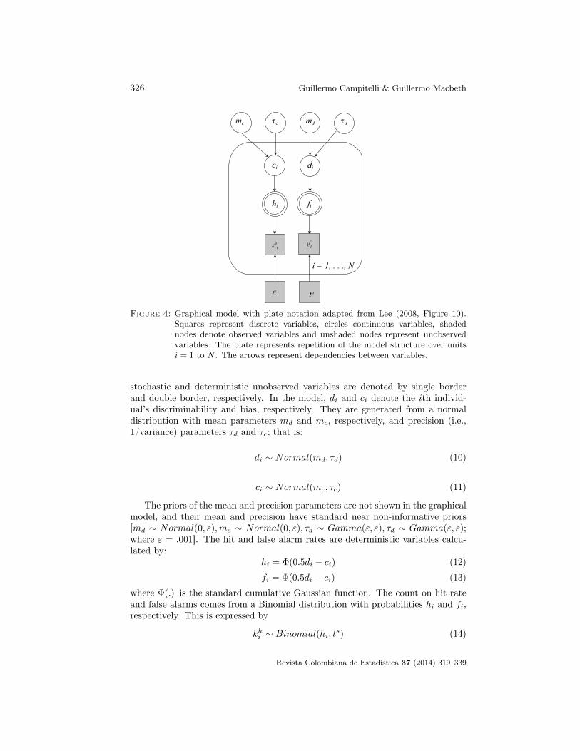
Lee (2011) indicated that Bayesian statistics have been used in psychology inthree ways. The first use of Bayesian statistics is to conduct data analysis. Ed-wards et al. (1963) introduced Bayesian analysis to psychology, and more recentlya number of researchers (Dienes 2011, Kruschke 2010a, Kruschke 2010b, Lee &Wagenmakers 2005, Wagenmakers 2007) have advocated that Bayesian statisticsshould replace the Null Hypothesis Statistical Testing (NHST) paradigm, whichis still the most popular paradigm in psychology. Another use of a Bayesian ap-proach in psychology is to produce psychological models of how humans makeinferences (see Griffiths, Kemp & Tenenbaum, 2008 for a detailed treatment ofthis approach). The third use –the one we focus on in this article–is to relatepsychological models to data. To our knowledge Lee (2008) presented the firstgraphical model with plates to represent hierarchical Bayesian models in psy-chology. Lee “translated” three influential cognitive models in psychology –themultidimensional scaling (MSD) representation of stimulus similarity (Shepard,1962, 1980), the generalized context model (GCM) account of category learning(Nosofsky, 1984, 1986), and a signal detection theory (SDT) account of reasoning(Heit & Rotello 2005)–into hierarchical Bayesian models. (see Figure 4).

The plate represents repetitions over N participants in a reasoning experiment(see 2005 Heit & Rotello for details of the experiment). Lee uses shaded nodes forobserved variables and nodes without shading for unobserved variables. Contin-uous variables are represented by circles and discrete variables with squares; and



mc τc

ci di

hi fi

i = 1, . . ., N

md τd

kfikh

i

tnts

Figure 4: Graphical model with plate notation adapted from Lee (2008, Figure 10).Squares represent discrete variables, circles continuous variables, shadednodes denote observed variables and unshaded nodes represent unobservedvariables. The plate represents repetition of the model structure over unitsi = 1 to N . The arrows represent dependencies between variables.

stochastic and deterministic unobserved variables are denoted by single borderand double border, respectively. In the model, di and ci denote the ith individ-ual’s discriminability and bias, respectively. They are generated from a normaldistribution with mean parameters md and mc, respectively, and precision (i.e.,1/variance) parameters τd and τc; that is:

di ∼ Normal(md, τd) (10)

ci ∼ Normal(mc, τc) (11)

The priors of the mean and precision parameters are not shown in the graphicalmodel, and their mean and precision have standard near non-informative priors[md ∼ Normal(0, ε),mc ∼ Normal(0, ε), τd ∼ Gamma(ε, ε), τd ∼ Gamma(ε, ε);where ε = .001]. The hit and false alarm rates are deterministic variables calcu-lated by:

hi = Φ(0.5di − ci) (12)

fi = Φ(0.5di − ci) (13)

where Φ(.) is the standard cumulative Gaussian function. The count on hit rateand false alarms comes from a Binomial distribution with probabilities hi and fi,respectively. This is expressed by

khi ∼ Binomial(hi, ts) (14)



kfi ∼ Binomial(fi, tn), (15)

where ts and tn are the number of signal and noise trials presented in the exper-iment. As in Buntine (1994) this graphical model uses shading to differentiateobserved from unobserved variables, and double border to represent deterministicvariables. A new aspect of this representation is that shape is used to differentiatecontinuous from discrete variables. Like Lunn et al. (2000), Lee (2008) indicatedthe unit index and the total number of repetitions, but he did not follow the for-mer in using double-edged arrows to denote a deterministic dependency betweenvariables. The distributions are not represented in the graphical model.

After Lee’s (2008) article the plate notation gained popularity within math-ematical psychology, and it has been subsequently used in a number of studies(e.g., Ahn, Krawitz, Kim, Busemeyer & Brown 2011, Bridwell, Hecker, Serences &Srinivasan 2013, Dyjas, Grasman, Wetzels, van der Maas & Wagenmakers 2012,Lee & Newell 2011, Lodewyckx, Kim, Lee, Tuerlinckx, Kuppens & Wagenmakers2011, Orhan & Jacobs 2013, Scheibehenne, Rieskamp & Wagenmakers 2013, Stey-vers, Lee & Wagenmakers 2009, van Ravenzwaaij, Moore, Lee & Newell 2014),and in the book “Bayesian Cognitive Modeling: A Practical Course” by Lee &Wagenmakers (2014).

5.2. Kruschke’s (2010) Hierarchical Bayesian GraphicalModels with Distribution Pictograms

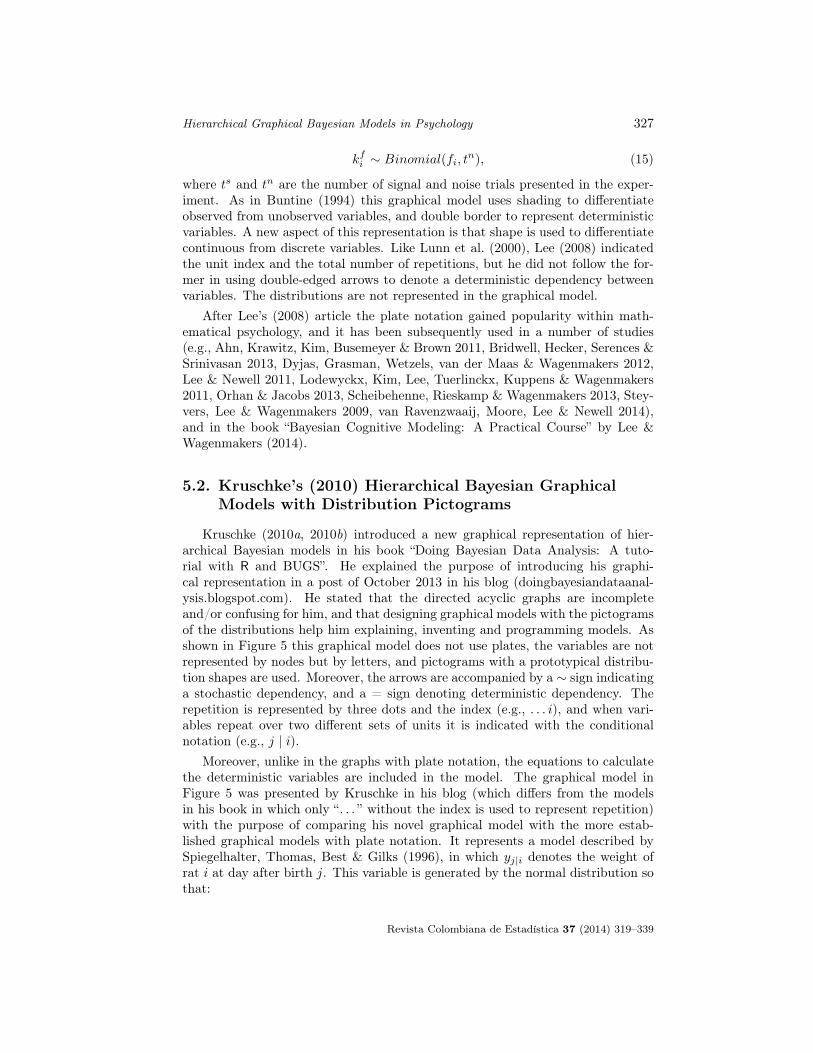
Kruschke (2010a, 2010b) introduced a new graphical representation of hier-archical Bayesian models in his book “Doing Bayesian Data Analysis: A tuto-rial with R and BUGS”. He explained the purpose of introducing his graphi-cal representation in a post of October 2013 in his blog (doingbayesiandataanal-ysis.blogspot.com). He stated that the directed acyclic graphs are incompleteand/or confusing for him, and that designing graphical models with the pictogramsof the distributions help him explaining, inventing and programming models. Asshown in Figure 5 this graphical model does not use plates, the variables are notrepresented by nodes but by letters, and pictograms with a prototypical distribu-tion shapes are used. Moreover, the arrows are accompanied by a ∼ sign indicatinga stochastic dependency, and a = sign denoting deterministic dependency. Therepetition is represented by three dots and the index (e.g., . . . i), and when vari-ables repeat over two different sets of units it is indicated with the conditionalnotation (e.g., j | i).

Moreover, unlike in the graphs with plate notation, the equations to calculatethe deterministic variables are included in the model. The graphical model inFigure 5 was presented by Kruschke in his blog (which differs from the modelsin his book in which only “. . . ” without the index is used to represent repetition)with the purpose of comparing his novel graphical model with the more estab-lished graphical models with plate notation. It represents a model described bySpiegelhalter, Thomas, Best & Gilks (1996), in which yj|i denotes the weight ofrat i at day after birth j. This variable is generated by the normal distribution sothat:



yj|i ∼ Normal(wj|i, λ), (16)

where wj|i is the mean and λ is the precision. wj|i is deterministically calculatedby

wj|i = φi + ξixj|i, (17)

where φi is the intercept and ξi is the slope, and both come from normal distribu-tions with means κ and ζ,; and precision δ and γ, respectively so that:

φi ∼ Normal(κ, δ) (18)

ξi ∼ Normal(ζ, γ) (19)

The mean parameters come from a normal distribution with priors M and H, andthe precisions come from a gamma distribution with parameters K and I.

M IH K

IK

M IH K

xj|i

...i...i

yj|i

...j|i

...j|i

normal

gamma

normal normal

normal

normal

gamma gamma

ξi

δ

φi

γ

ωj|i

κ

λ

ζ

~ ~

~

~

~

~

~

~

+ .

=

Figure 5: Adaptation of the type of graphical model representation introduced by Kr-uschke (2010a, 2010b). Stochastic variables are represented by small letterswhich are generated by a distribution (represented by pictograms) with thecorresponding parameters. Stochastic variables are represented with smallletters, and their values are computed by the corresponding equation. Ar-rows with the sign ∼ denote stochastic dependencies, and arrows with thesign= represent deterministic dependencies. The pictograms were generatedusing Bååth’s (2013) template for LibreOffice.

This graphical representation was subsequently used by Kruschke and his col-leagues (e.g., Kruschke 2013, Kruschke, Aguinis & Joo 2012). Bååth (2013) createda script in R (R Development Core Team 2013) to produce Kruschke’s distribu-tion pictograms and a template for the LibreOffice (Document Foundation, 2013)



Figure 6: Adaptation of Schneider’s (2013) representation of Kruschke’s (2010) stylegraphical models. We generated the pictograms with Bååth’s (2013) templatefor LibreOffice. The shapes surrounding the distributions are not plates, theyonly emphasise to which distribution the parameters belong to.

free software to draw the graphical diagrams with the distribution pictograms.Schneider (2013) presented a graphical model using Bååth’s pictograms. This rep-resentation differs from that of Kruschke in that boxes were added around thedistributions and double-edge arrows were used to denote deterministic relations.(Note that instead of the single-edged arrow used in Figure 6, Schneider used acurly arrow), and the deterministic equation is surrounded by a brace. Summingup, Kruschke’s (2010a, 2010b) graphical model puts emphasis on the type of dis-tribution. The repetition is not represented by plates, rather three dots and theindices of the variables are presented to denote the repetition. Another importantaspect of this graphical model is that the parameters that belong to the samedistribution are presented contiguously in space. (Note that this is even moreemphasized in Schneider’s representation, in which the parameters that form adistribution are surrounded by a box). As indicated by Kruschke the inclusion ofdistribution pictograms plays a heuristic role for the invention, explanation andprogramming of models. A possible problem with this approach is that sometimesa deterministic variable comes from a long relation between other variables, whichcould use a lot of space and make the graph difficult to understand.

6. Discussion

Both the graphical models with plates and the graphical models with distri-bution pictograms share the importance of representing the dependencies betweenvariables by using arrows. The former emphasise the independent repetition of thevariables, and the latter emphasises the probabilistic distributions. As mentionedearlier, Buntine’s (1994) graphical models contained both plates and the names



(instead of the pictograms) of the distributions. However, Buntine only presentedgraphical models with one or two plates, and the larger the number of plates thesmaller the space to include information about the distribution.

Moreover, complex models are also difficult to represent with graphical modelswith plates. For example, Figure 6.3 shows a hierarchical Bayesian model presentedby Lee (2008). The complexity of the model led the author to use three i platesand two j plates. Although this solution is flawless from the formal point of view,it reduces the heuristic value of the graphical models with plates. Given thatthere is no differentiation between plates (i.e., they all have the same format)the only graphical difference between, say the plate i and the plate j is thatthey are different plates. Therefore, adding more plates for denoting repetitionover the same set of units might be confusing for some researchers. One obvioussolution to this problem is to colour code or shape code the plates. That is, touse a different colour (or shape) for each type of plate. Based on this summarywe aimed at developing a type of graphical model that incorporates both thedistribution pictograms and the plate notation, that solves the problems identifiedin the discussion, and that it has heuristic value to help researchers invent, explainand program hierarchical Bayesian models.

6.1. Hierarchical Bayesian Graphical Models withDistribution Pictograms and Mini-Plates

The first ingredient of our proposal is the replacements of plates by colour-coded mini-plates. (Note that in the paper version of this article we use shadings;please refer to the link provided below to see a colour version of the graphicalmodels). As explained above, the purpose of colour-coding is to graphically dif-ferentiate between different types of plates. While we were developing the idea ofusing colour to differentiate between plates we realise that if the colour indicatesthe set of units over which the repetition occurs then the plates might not be nec-essary. Thus, we originally developed graphical models without plates in whichwe colour coded the nodes. However, because colour (or shading) is already usedto code for variable type (i.e., observed vs. unobserved) this implementation wasunsatisfactory.

That led us to develop the idea of colour coded mini-plates, and use them tosurround each node. However, this was also unsatisfactory because the mini-plateswith the nodes occupied too much space. In parallel we were also considering theuse of 3D representations in order to make the graphical models more attractive.When we were trying different ways of using 3D nodes we found out that in somecases the combination of 3D shapes occupy less space than 2D shapes because theformer allow more flexibility to locate the nodes in space. Thus, we realised thatusing 3D nodes was also a good idea to save space, and then we came up with theidea of using 3D rotated mini-plates under the nodes, instead of surrounding thenodes.

Unfortunately, in order to trigger the perception of 3D nodes it is necessaryto add some shading to the nodes, which, as indicated by a reviewer, was very



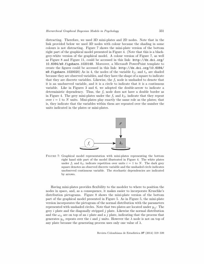
distracting. Therefore, we used 3D mini-plates and 2D nodes. Note that in thelink provided below we used 3D nodes with colour because the shading in somecolours is not distracting. Figure 7 shows the mini-plate version of the bottomright part of the graphical model presented in Figure 4. (Note that this is a black-grey-white version of the graphical model. A colour version of Figure 7, as wellas Figure 8 and Figure 11, could be accessed in this link: http://dx.doi.org/10.6084/m9.figshare.1020148. Moreover, a Microsoft PowerPoint template tocreate the figures could be accessed in this link: http://dx.doi.org/10.6084/m9.figshare.1020020) As in 4, the nodes of the variable kfi and tn are shadedbecause they are observed variables, and they have the shape of a square to indicatethat they are discrete variables. Likewise, the fi node is unshaded to denote thatit is an unobserved variable, and it is a circle to indicate that it is a continuousvariable. Like in Figures 3 and 6, we adopted the double-arrow to indicate adeterministic dependency. Thus, the fi node does not have a double border asin Figure 4. The grey mini-plates under the fi and kfi indicate that they repeatover i = 1 to N units. Mini-plates play exactly the same role as the plates; thatis, they indicate that the variables within them are repeated over the number theunits indicated in the plates or mini-plates.

fi

tn

kf i

Figure 7: Graphical model representation with mini-plates representing the bottomright hand side part of the model illustrated in Figure 4. The white platesunder fi and kfi indicate repetition over units i = 1 to N . The dark greysquare denotes an observed discrete variable and the unshaded circle indicatesunobserved continuous variable. The stochastic dependencies are indicatedby arrows.

Having mini-plates provides flexibility to the modeler to where to position thenodes in space, and, as a consequence, it makes easier to incorporate Kruschke’sdistribution pictograms. Figure 8 shows the mini-plate version of the bottompart of the graphical model presented in Figure 5. As in Figure 5, the mini-plateversion incorporates the pictogram of the normal distribution with the parametersrepresented with unshaded circles. Note that two plates are located under yij : Thegrey i plate and the diagonally stripped j plate. Likewise the normal distributionand the ωij are on top of an i plate and a j plate, indicating that the process thatgenerates yij repeats over the i and j units. However the λ node is not on top ofany plate because the generating process uses only one value of λ.


http://dx.doi.org/10.6084/m9.figshare.1020148





Figure 8: Graphical model with mini-plates and distribution pictograms representingthe bottom part of Figure 5. The white plate under yij and ωij indicate thatthese variables repeat over i = 1 to N units. The diagonally stripped platesunder the same variables denote their repetition over j = 1 to M units. λ isa parameter of the normal distribution, and given that it is not located ontop of plates, it does not repeat itself.

6.2. Comparison Between Three Graphical ModelRepresentations of a Hierarchical Bayesian Model

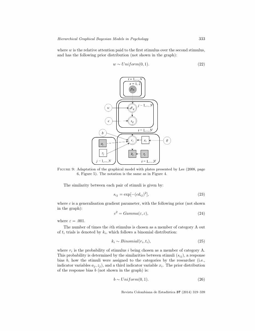
Having presented the mini-plate with distribution pictograms, we now discusswhether this type of graphical representation is capable of representing complexmodels, and how it compares with the other two types of graphical models. Forthis purpose we present here a complex hierarchical Bayesian model with plate no-tation developed by Lee (2008, pages 5 to 8), based on Nosofsky (1986) generalisedcontext model (GCM) of category learning.

This model aims at explaining how people learn to categorise unknown stimuliinto two categories in experiments in which the researcher uses different categorystructures (see more details in Lee, 2008). In those experiments the researcherassigns one fourth of the total number of stimuli to one category (i.e., categoryA), one fourth to the other category (i.e., category B), and one half is not assignedto any category. The model utilises the multidimensional scaling (MDS) represen-tation of stimulus similarity developed by Shepard (1962). Stimuli are representedas points (p) in a D-dimensional space. In Figure 9 pix denotes a coordinate valueof stimulus i in dimension x. The surrounding plates indicates that, in this exam-ple, there are N stimuli and x = 2 dimensions. Lee (2008) assigned the followingprior probability to pix (not shown in the graph):

pix ∼ Uniform(−δ, δ); δ > 0, (20)

d2ij denotes the squared psychological distance between all the possible pairs of Nstimuli, where i denotes the first stimulus and j the second stimulus of the pair.The node is surrounded by the i and j plates to denote the repetition over all thepossible pairs of stimuli. The squared psychological distance between stimuli isdetermined by:

d2ij = w(pi1 − pj1)2 + (1− w)(pi2 − pj2)2, (21)



where w is the relative attention paid to the first stimulus over the second stimulus,and has the following prior distribution (not shown in the graph):

w ∼ Uniform(0, 1). (22)

Figure 9: Adaptation of the graphical model with plates presented by Lee (2008, page6, Figure 5). The notation is the same as in Figure 4.

The similarity between each pair of stimuli is given by:

sij = exp[−(cdij)2], (23)

where c is a generalisation gradient parameter, with the following prior (not shownin the graph):

c2 = Gamma(ε, ε), (24)

where ε = .001.The number of times the ith stimulus is chosen as a member of category A out

of ti trials is denoted by ki, which follows a binomial distribution:

ki ∼ Binomial(ri, ti), (25)

where ri is the probability of stimulus i being chosen as a member of category A.This probability is determined by the similarities between stimuli (sij), a responsebias b, how the stimuli were assigned to the categories by the researcher (i.e.,indicator variables aj , zj), and a third indicator variable xi. The prior distributionof the response bias b (not shown in the graph) is:

b ∼ Uniform(0, 1). (26)



aj denotes the known assignment of the jth presented stimulus, which rangesover N/2 such stimuli, and zj indicates the latent assignment of the jth unassignedstimulus, ranging over the N/2 such stimuli (see Lee, 2008, for a more detailedexplanation of stimuli assignment structures), with the following prior:

zj ∼ Bernoulli(1/2). (27)

The xi is incorporated in the graph in order to compare a model that uses thelatent stimulus assignment zj with a simpler model without this latent variable.xi indicates for each stimulus i whether the response probability ri uses aj andzj (i.e., xi = 1) or only aj (i.e., xi = 0). It is assumed that all the indicatorsxi support either model following a fixed underlying rate of use (i.e., θ), which isgiven by the following prior:

θ ∼ Uniform(0, 1). (28)

The posterior rate of use provides information on how well each model accountsfor the categorisations of the participants (for a more detailed explanation see Lee,2008, page 8). Finally, the probability for the ith stimulus to be classified as amember of category A is given by:

ri =b∑aεA sia

b∑aεA sia + (1− b)

∑aεB sia

, (29)

if xi is 0.

ri =b[∑aεA sia +

∑zεA siz]

b[∑aεA sia +

∑zεA siz] + (1− b)[

∑aεB sia +

∑zεB siz]

, (30)

if xi is 1.Figure 9 shows Lee’s (2008) graphical model with plates, 10 presents our best

attempt to represent the same model with the graphical model with distributionpictograms proposed by Kruschke (2010a), and Figure 11 depicts the graphicalmodel with mini-plates and distribution pictograms, as proposed in this arti-cle. Regarding the amount of information presented, Kruschke’s graphical modelpresents more information (equations, distributions, dependencies and repetitions)than the mini-plate graphical model (distributions, dependencies and repetitions)and the plate graphical model (dependencies and distributions). However, it seemsto us that the inclusion of equations in Kruschke’s graphical model attemptsagainst the heuristic value of the model by cluttering the space with too muchinformation. Possibly, Kruschke’s style graphical model should include equationsonly when the models are simple and exclude them when the models contain morethan one or two equations and/or when the equations are large.

The mini-plate graphical representation seems to strike a balance betweenamount of information and use of space. By using the concept of plates in a flexibleway (i.e., mini-plates), combining them with Kruschke’s distribution pictograms,and using 3D shapes it has a strong visual appeal. However, this comparisonis not completely fair for the other graphical representations. As we mentioned



Figure 10: Graphical model with Kruschke’s style distribution pictograms of the hier-archical Bayesian model presented by Lee (2008, pages 5 to 8). The notationis the same as in Figure 5.

Figure 11: Graphical model with mini-plates of the hierarchical Bayesian model pre-sented by Lee (2008, pages 5 to 8). The notation is the same as in Figure8.

above, Kruschke’s graphical models could be improved by not including equationsin complex models, and we might not have done the best to present the best pos-sible representation. Moreover, there are a variety of plate graphical models thatwe are not displaying in this article. For example, van Ravenzwaaij et al. (2014)



presented a plate graphical model following Lee’s (2008) notation, but in the righthand side of the figure they added both the distributions and the equations intext format. Allegedly, this might be a better representation than the mini-plategraphical models because it combines graphical aspects with text, rather thanbeing too graphical.

7. Conclusion

We discussed two types of hierarchical Bayesian graphical models used in psy-chology –Lee’s (2008) plate graphical models and Kruschke’s (2010b) graphicalmodels with distribution pictograms. We proposed a third type– graphical mod-els with colour-coded mini-plates– as an attempt to combine the positive aspectsof the other two types of graphical models, and we presented a preliminary in-tuitive analysis of the informative value of this new graphical respresentation.We believe our proposal provides an important contribution to the field, but ourintuitive evaluation should be confirmed by empirical evidence. Statistical cogni-tion is a flourishing area of research in psychology (e.g., Beyth Marom, Fidler &Cumming 2008), that investigates how people understand statistical information.Our proposal could be followed up by a research that aims at elucidating whichtype of graphical model leads to a better understanding of hierarchical Bayesianmodels. [

Recibido: mayo de 2014 — Aceptado: septiembre de 2014]

References

Ahn, W.-Y., Krawitz, A., Kim, W., Busemeyer, J. R. & Brown, J. W. (2011),‘A model-based FMRI analysis with hierarchical Bayesian parameter estima-tion’, Journal of Neuroscience, Psychology, and Economics 4(2), 95–110.

Bauer, M. I. & Johnson-Laird, P. N. (1993), ‘How diagrams can improve reasoning’,Psychological Science 4(6), 372–378.

Beyth Marom, R., Fidler, F. & Cumming, G. (2008), ‘Statistical cognition: To-wards evidence-based practice in statistics and statistics education’, StatisticsEducation Research Journal 7(2), 20–39.

Bolstad, W. M. (2007), Introduction to Bayesian Statistics, 2 edn, Wiley Jobs inHoboken, New York.

Bridwell, D. A., Hecker, E. A., Serences, J. T. & Srinivasan, R. (2013), ‘Individualdifferences in attention strategies during detection, fine discrimination, andcoarse discrimination’, Journal of Neurophysiology 110, 784–794.

Bååth, R. (2013), Distribution diagram R scripts.*https://github.com/rasmusab/distribution_diagrams



Buntine, W. L. (1994), ‘Operations for learning with graphical models’, Journalof Artificial Intelligence Research 2, 159–225.

Dienes, Z. (2011), ‘Bayesian versus orthodox statistics: Which side are you on?’,Perspectives on Psychological Science 6, 274–290.

Dyjas, O., Grasman, R. P., Wetzels, R., van der Maas, H. L. & Wagenmakers, E.(2012), ‘A Bayesian hierarchical analysis of the name-letter effect’, Frontiersin Psychology 3(334), 1–14. doi: 10.3389/fpsyg.2012.00334.

Edwards, W., Lindman, H. & Savage, L. J. (1963), ‘Bayesian statistical inferencefor psychological research’, Psychological Review 70, 193–242.

Gilks, W. R., Thomas, A. & Spiegelhalter, D. J. (1994), ‘A language and programfor complex Bayesian modelling’, The Statistician 43, 169–177.

Good, I. J. (1980), ‘Some history of the hierarchical Bayesian methodology’, Tra-bajos de Estadística y de Investigación Operativa 31(1), 489–519.

Gray, K. & Wegner, D. M. (2013), ‘Six guidelines for interesting research’, Per-spectives on Psychological Science 8(5), 549–553.

Griffiths, T. L., Kemp, C. & Tenenbaum, J. B. (2008), Bayesian models of cogni-tion, in R. Sun, ed., ‘The Cambridge Handbook of Computational Psychol-ogy’, Cambridge University Press, Cambridge, New York, pp. 59–100.

Heit, E. & Rotello, C. (2005), Are there two kinds of reasoning?, in B. G. Bara,L. W. Barsalou & M. Bucciarelli, eds, ‘Proceedings of the 27th Annual Con-ference of the Cognitive Science Society’, Lawrence, Erlbaum, Mahwah, NewJersey.

Jordan, M. I. (2004), ‘Graphical models’, Statistical Science 19, 140–155.

Koller, D. & Friedman, N. (2009), Probabilistic Graphical Models: Principles andTechniques, MIT press, Cambridge, MA.

Koller, D., Friedman, N., Getoor, L. & Taskar, B. (2007), Graphical models in anutshell, in L. Getoor & B. Taskar, eds, ‘Introduction to statistical relationallearning’, MIT Press, Cambridge, Massachusetts.

Kruschke, J. K. (2010a), Doing Bayesian Data Analysis: A Tutorial with R andBUGS, Academic Press, Burlington, MA.

Kruschke, J. K. (2010b), ‘What to believe: Bayesian methods for data analysis’,Trends in Cognitive Science 14, 293–300.

Kruschke, J. K. (2013), ‘Bayesian estimation supersedes the t test’, Journal ofExperimental Psychology: General 142, 573–603.

Kruschke, J. K., Aguinis, H. & Joo, H. (2012), ‘The time has come: Bayesianmethods for data analysis in the organizational sciences’, Organizational Re-search Methods 15, 722–752.



Lee, M. D. (2008), ‘Three case studies in the Bayesian analysis of cognitive models’,Psychonomic Bulletin and Review 15, 1–15.

Lee, M. D. (2011), ‘How cognitive modeling can benefit from hierarchical Bayesianmodels’, Journal of Mathematical Psychology 55, 1–7.

Lee, M. D. & Newell, B. R. (2011), ‘Using hierarchical Bayesian methods to exam-ine the tools of decision-making’, Judgment and Decision Making 6, 832–842.

Lee, M. D. & Wagenmakers, E.-J. (2005), ‘Postscript: Bayesian statistical in-ference in psychology: Comment on Trafimow (2003)’, Psychological Review112(3), 662–668.

Lee, M. D. & Wagenmakers, E.-J. (2014), ‘Bayesian cognitive modeling: A prac-tical course’, New York: Cambridge University Press .

Lodewyckx, T., Kim, W., Lee, M. D., Tuerlinckx, F., Kuppens, P. &Wagenmakers,E. J. (2011), ‘A tutorial on Bayes factor estimation with the product spacemethod’, Journal of Mathematical Psychology 55, 331–347.

Lunn, D. J., Thomas, A., Best, N. & Spiegelhalter, D. (2000), ‘A Bayesian mod-elling framework: Concepts, structure, and extensibility’, Statistics and Com-puting 10, 325–337.

Nosofsky, R. M. (1984), ‘Choice, similarity, and the context theory of classifica-tion’, Journal of Experimental Psychology: Learning, Memory and Cognition10, 104–114.

Nosofsky, R. M. (1986), ‘Attention, similarity, and the identifica-tion–categorization relationship’, Journal of Experimental Psychology:General 115, 39–57.

Orhan, A. E. & Jacobs, R. A. (2013), ‘A probabilistic clustering theory of theorganization of visual short-term memory’, Psychological Review 120, 297–328.

Pearl, J. (2009), ‘Causal inference in statistics: An overview’, Statistics Surveys3, 96–146.

R Development Core Team (2013), R: A Language and Environment for StatisticalComputing, R Foundation for Statistical Computing, Vienna, Austria. ISBN3-900051-07-0.*http://www.R-project.org

Scheibehenne, B., Rieskamp, J. & Wagenmakers, E.-J. (2013), ‘Testing adap-tive toolbox models: A Bayesian hierarchical approach’, Psychological Review120, 39–64.

Schneider, T. (2013), Diagram for Hierarchical Models.*https://github.com/tinu-schneider/DBDA_hierach_diagram



Shepard, R. N. (1962), ‘The analysis of proximities: Multidimensional scaling withan unknown distance function. I’, Psychometrika 27(2), 125–140.

Shepard, R. N. (1980), ‘Multidimensional scaling, tree-fitting, and clustering’, Sci-ence 210, 390–398.

Spiegelhalter, D., Thomas, A., Best, N. & Gilks, W. (1996), BUGS 0.5* ExamplesVolume 2 (version ii), 2 edn, MRC Biostatistics Unit.

Stenning, K. & Oberlander, J. (1995), ‘A cognitive theory of graphical and linguis-tic reasoning: Logic and implementation’, Cognitive Science 19(1), 97–140.

Steyvers, M., Lee, M. D. & Wagenmakers, E.-J. (2009), ‘Bayesian analysis ofhuman decision-making on bandit problems’, Journal of Mathematical Psy-chology 53(3), 168–179.

van Ravenzwaaij, D., Moore, C. P., Lee, M. D. & Newell, B. R. (2014), ‘A hierarchi-cal Bayesian modeling approach to searching and stopping in multi-attributejudgment’, Cognitive Science 38, 1384–1405.

Wagenmakers, E. (2007), ‘A practical solution to the pervasive problems of pvalues’, Psychonomic Bulletin and Review 14, 779–804.

Wickens, C. D., Merwin, D. H. & Lin, E. L. (1994), ‘Implications of graphicsenhancements for the visualization of scientific data: Dimensional integrality,stereopsis, motion, and mesh’, Human Factors 36(1), 44–61.


Documents

Hierarchical Graphical Bayesian Models in Psychology · Hierarchical Graphical Bayesian Models in Psychology 321 isaprobabilitythatananimalbelongstoacategoryofanimal(e.g.,mammal),a