INDUSTRIAL ROBOTICS Prof. Bruno SICILIANO
DIFFERENTIAL KINEMATICS
• relationship between joint velocities and end-effector velocities
Geometric Jacobian
Analytical Jacobian
Kinematic singularities
Kinematic redundancy
Inverse differential kinematics
Inverse kinematics algorithms
STATICS
• relationship between end-effector forces and joint torques
INDUSTRIAL ROBOTICS Prof. Bruno SICILIANO
GEOMETRIC JACOBIAN
T (q) =
R(q) p(q)
0T 1
• Goal
p = JP (q)q
ω = JO(q)q
v =
[
p
ω
]
= J(q)q
INDUSTRIAL ROBOTICS Prof. Bruno SICILIANO
Derivative of a rotation matrix
R(t)RT (t) = I
R(t)RT (t) + R(t)RT (t) = O
• Given S(t) = R(t)RT (t)
S(t) + ST (t) = O
R(t) = S(ω(t))R(t)
S =
0 −ωz ωy
ωz 0 −ωx
−ωy ωx 0
INDUSTRIAL ROBOTICS Prof. Bruno SICILIANO
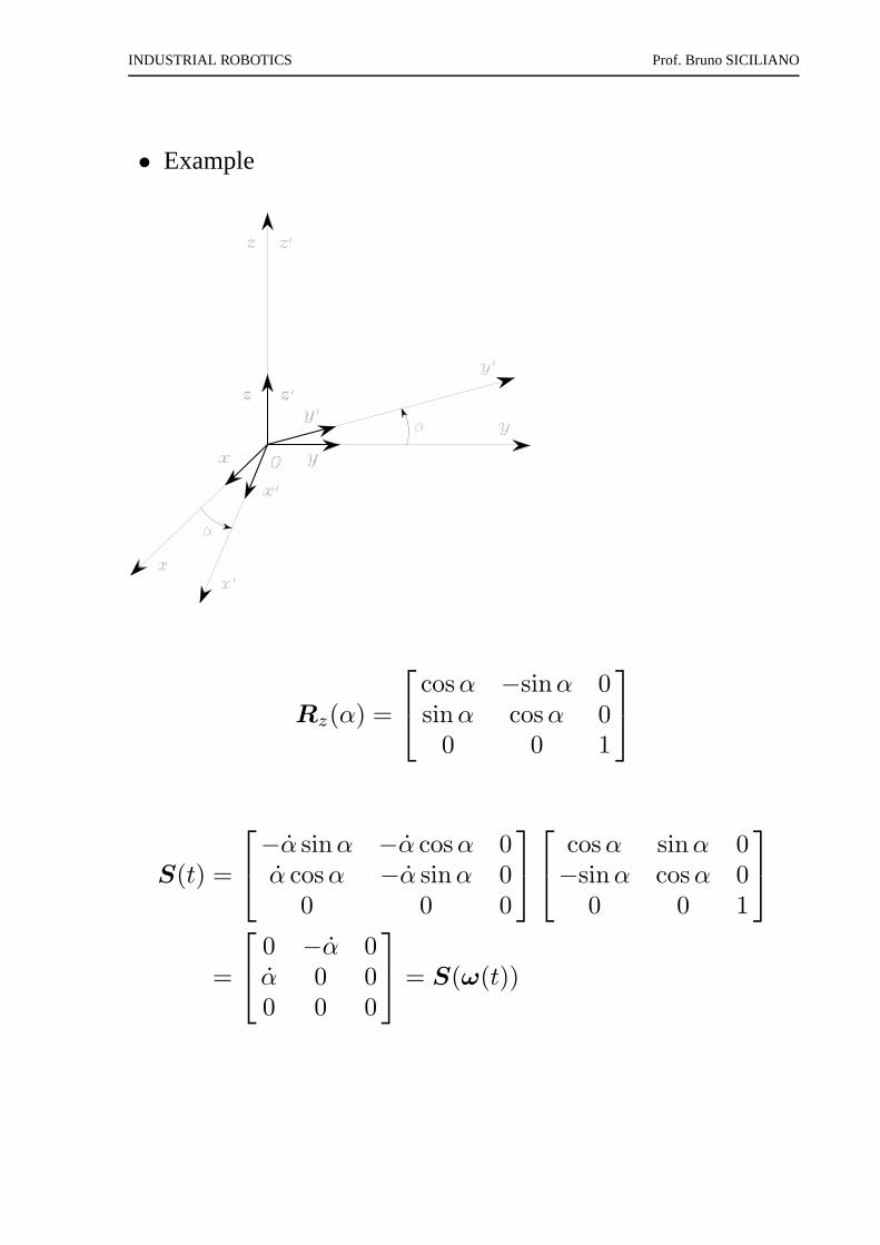
• Example
Rz(α) =
cosα −sinα 0sinα cosα 0
0 0 1
S(t) =
−α sinα −α cosα 0α cosα −α sinα 0
0 0 0
cosα sinα 0−sinα cosα 0
0 0 1
=
0 −α 0α 0 00 0 0
= S(ω(t))
INDUSTRIAL ROBOTICS Prof. Bruno SICILIANO
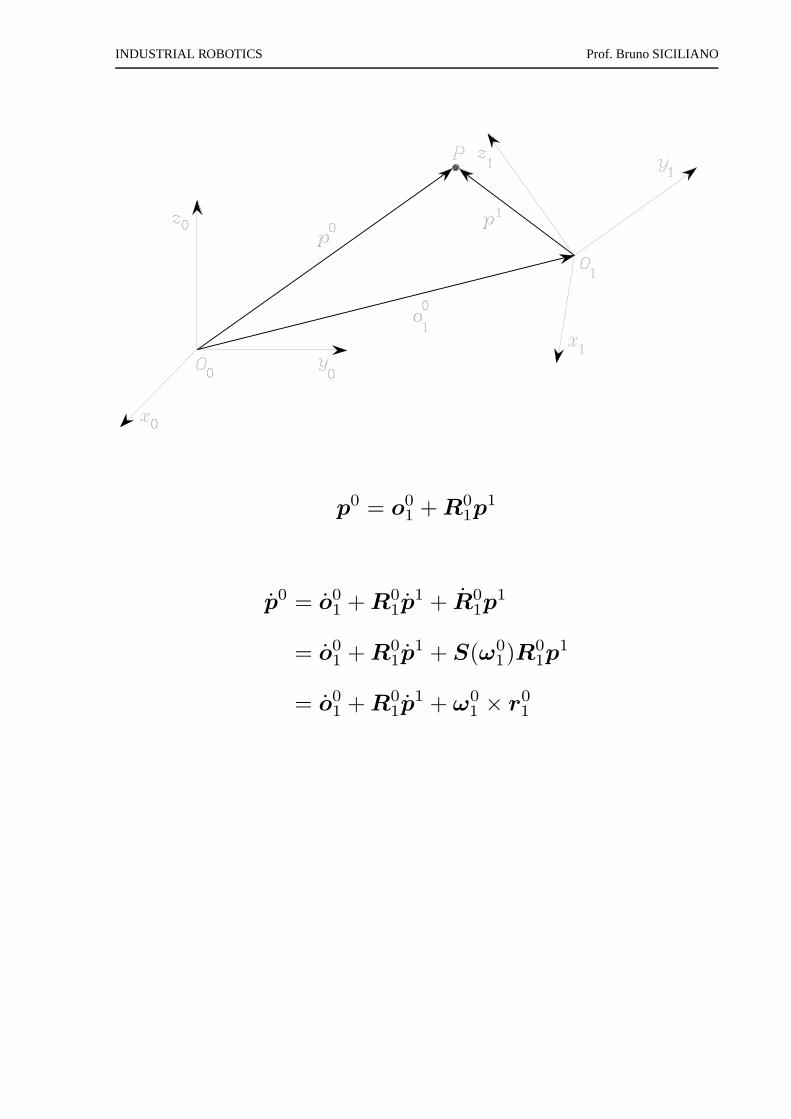
p0 = o01 + R0
1p1
p0 = o01 + R0
1p1 + R0
1p1
= o01 + R0
1p1 + S(ω0
1)R01p
1
= o01 + R0
1p1 + ω0
1 × r01
INDUSTRIAL ROBOTICS Prof. Bruno SICILIANO
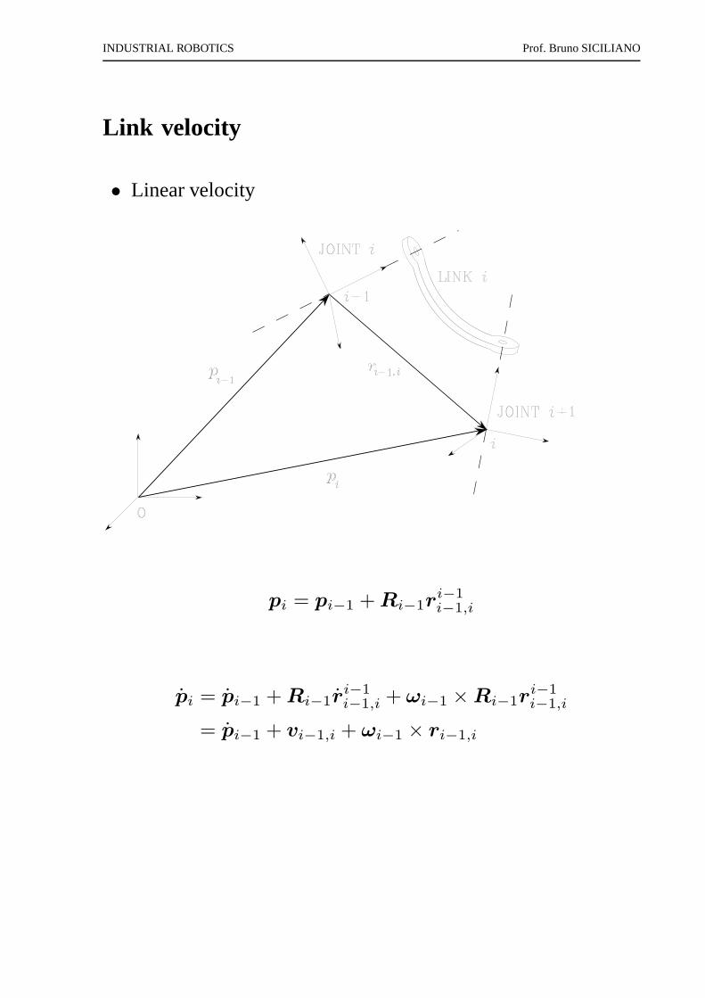
Link velocity
• Linear velocity
pi = pi−1 + Ri−1ri−1
i−1,i
pi = pi−1 + Ri−1ri−1
i−1,i + ωi−1 × Ri−1ri−1
i−1,i
= pi−1 + vi−1,i + ωi−1 × ri−1,i
INDUSTRIAL ROBOTICS Prof. Bruno SICILIANO
• Angular velocity
Ri = Ri−1Ri−1
i
S(ωi)Ri = S(ωi−1)Ri + Ri−1S(ωi−1
i−1,i)Ri−1
i
= S(ωi−1)Ri + S(Ri−1ωi−1
i−1,i)Ri
ωi = ωi−1 + Ri−1ωi−1
i−1,i
= ωi−1 + ωi−1,i
INDUSTRIAL ROBOTICS Prof. Bruno SICILIANO
ωi = ωi−1 + ωi−1,i
pi = pi−1 + vi−1,i + ωi−1 × ri−1,i
• Prismatic joint
ωi−1,i = 0
vi−1,i = dizi−1
ωi = ωi−1
pi = pi−1 + dizi−1 + ωi × ri−1,i
• Revolute joint
ωi−1,i = ϑizi−1
vi−1,i = ωi−1,i × ri−1,i
ωi = ωi−1 + ϑizi−1
pi = pi−1 + ωi × ri−1,i
INDUSTRIAL ROBOTICS Prof. Bruno SICILIANO
Jacobian computation
J =
P1 Pn
. . .O1 On
• Angular velocity
⋆ Jointi prismatic
qiOi = 0 =⇒ Oi = 0
⋆ Jointi revolute
qiOi = ϑizi−1 =⇒ Oi = zi−1
INDUSTRIAL ROBOTICS Prof. Bruno SICILIANO
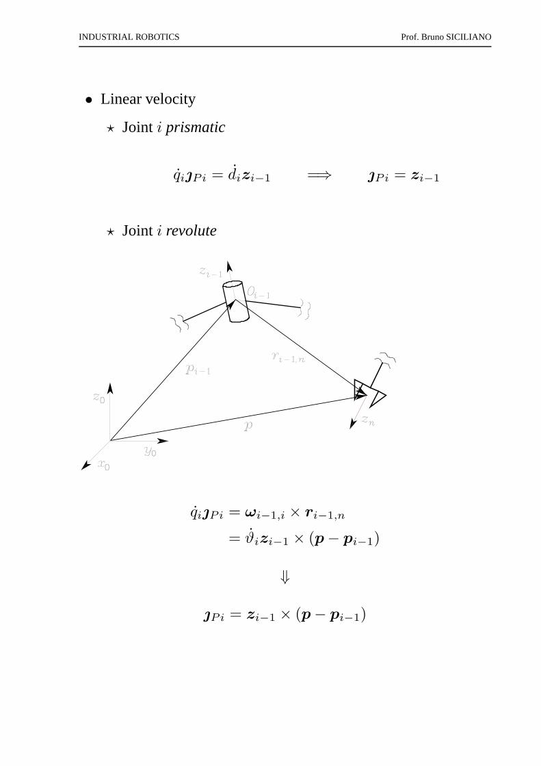
• Linear velocity
⋆ Jointi prismatic
qiPi = dizi−1 =⇒ Pi = zi−1
⋆ Jointi revolute
qiPi = ωi−1,i × ri−1,n
= ϑizi−1 × (p − pi−1)
⇓
Pi = zi−1 × (p − pi−1)
INDUSTRIAL ROBOTICS Prof. Bruno SICILIANO
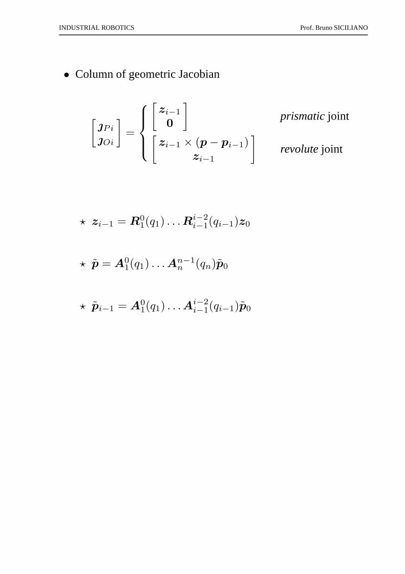
• Column of geometric Jacobian
[
Pi
Oi
]
=
[
zi−1
0
]
prismaticjoint[
zi−1 × (p − pi−1)zi−1
]
revolutejoint
⋆ zi−1 = R01(q1) . . .R
i−2
i−1(qi−1)z0
⋆ p = A01(q1) . . .A
n−1n (qn)p0
⋆ pi−1 = A01(q1) . . .A
i−2
i−1(qi−1)p0
INDUSTRIAL ROBOTICS Prof. Bruno SICILIANO
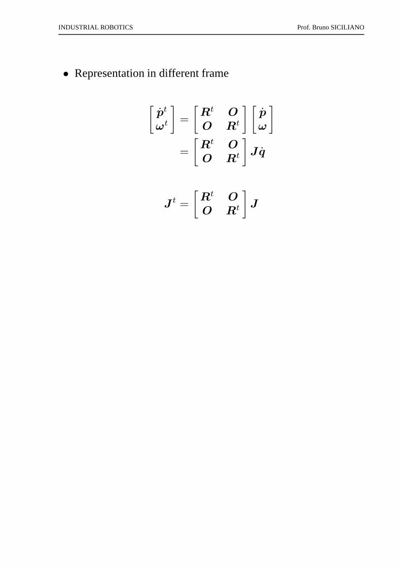
• Representation in different frame
[
pt
ωt
]
=
[
Rt O
O Rt
] [
p
ω
]
=
[
Rt O
O Rt
]
Jq
J t =
[
Rt O
O Rt
]
J
INDUSTRIAL ROBOTICS Prof. Bruno SICILIANO
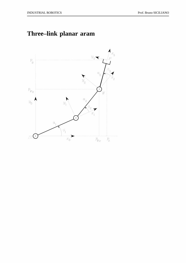
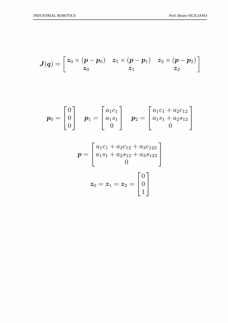
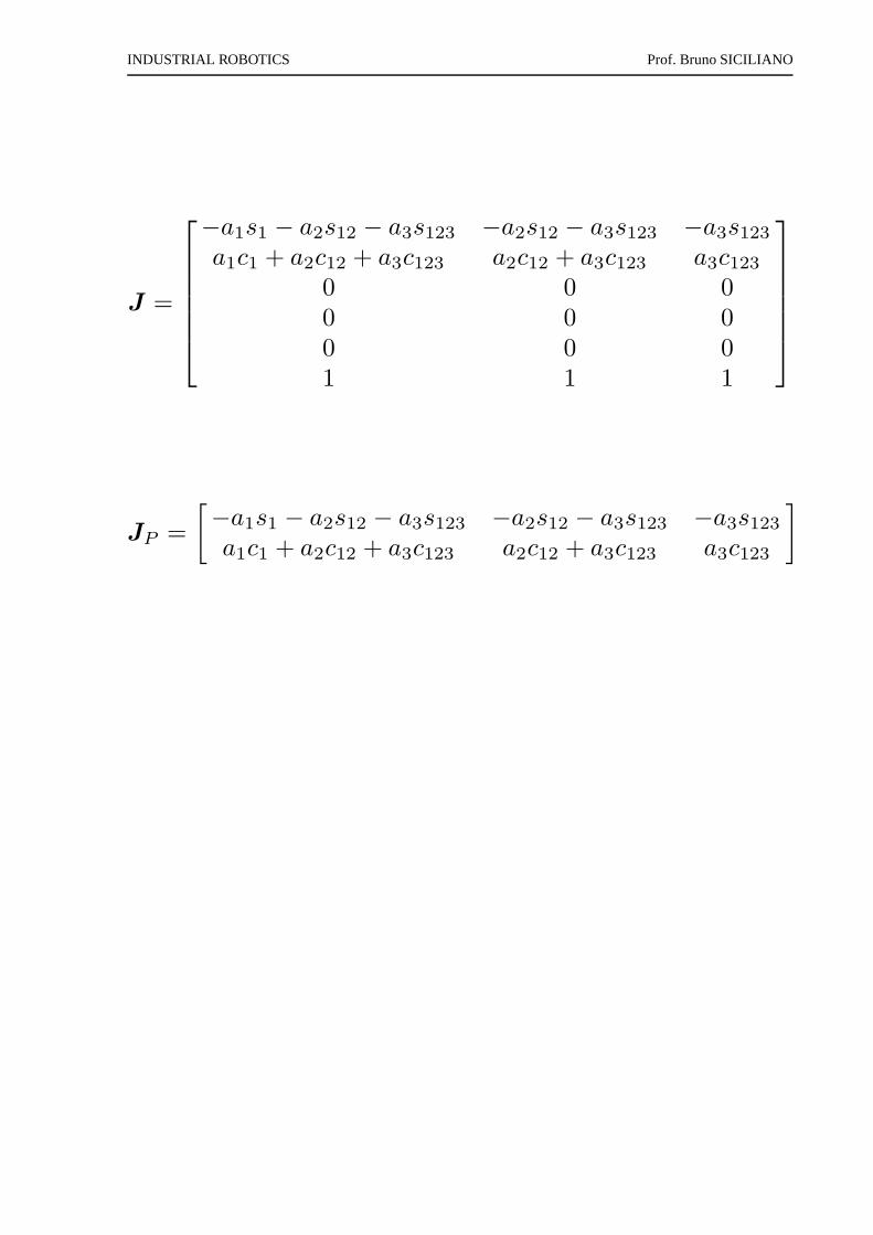
Three–link planar aram
INDUSTRIAL ROBOTICS Prof. Bruno SICILIANO
J(q) =
[
z0 × (p − p0) z1 × (p − p1) z2 × (p − p2)z0 z1 z2
]
p0 =
000
p1 =
a1c1a1s1
0
p2 =
a1c1 + a2c12a1s1 + a2s12
0
p =
a1c1 + a2c12 + a3c123a1s1 + a2s12 + a3s123
0
z0 = z1 = z2 =
001
INDUSTRIAL ROBOTICS Prof. Bruno SICILIANO
J =
−a1s1 − a2s12 − a3s123 −a2s12 − a3s123 −a3s123a1c1 + a2c12 + a3c123 a2c12 + a3c123 a3c123
0 0 00 0 00 0 01 1 1
JP =
[
−a1s1 − a2s12 − a3s123 −a2s12 − a3s123 −a3s123a1c1 + a2c12 + a3c123 a2c12 + a3c123 a3c123
]
INDUSTRIAL ROBOTICS Prof. Bruno SICILIANO
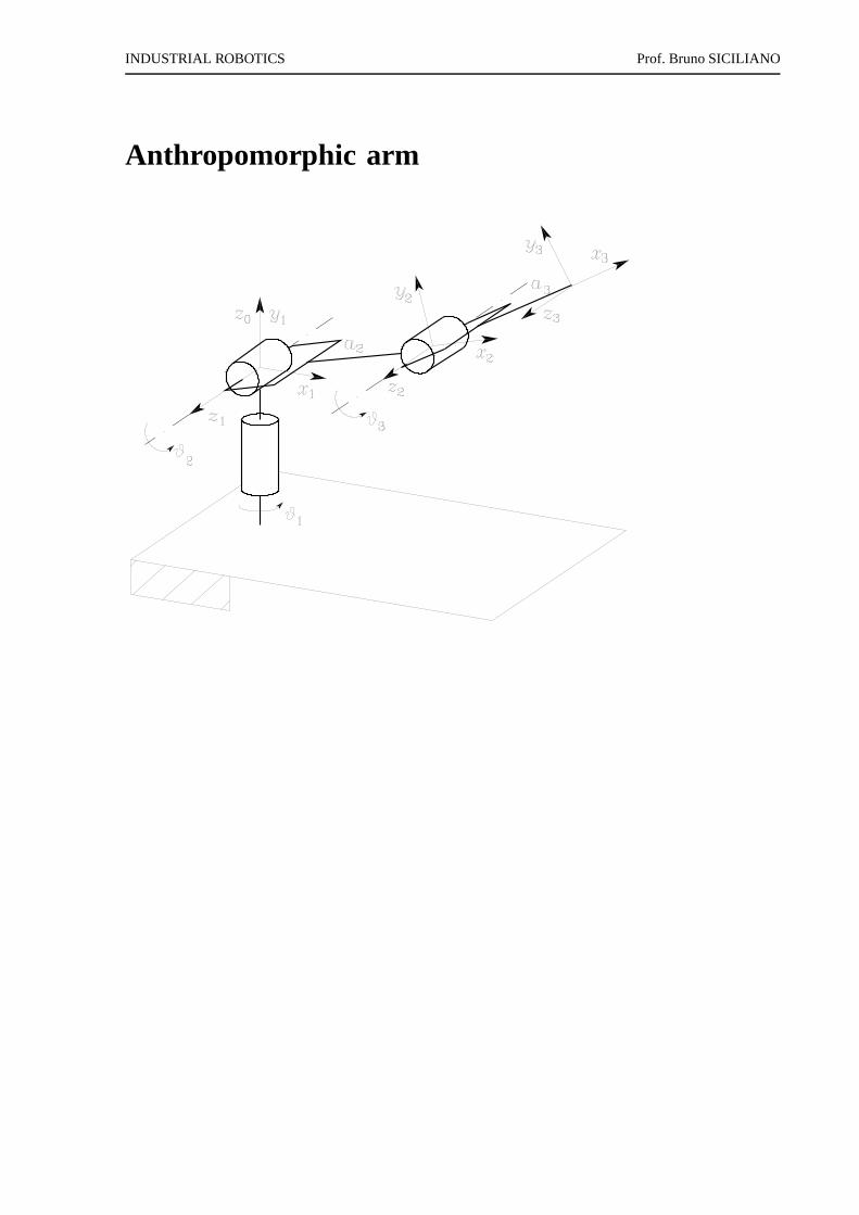
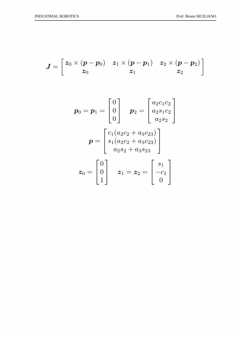
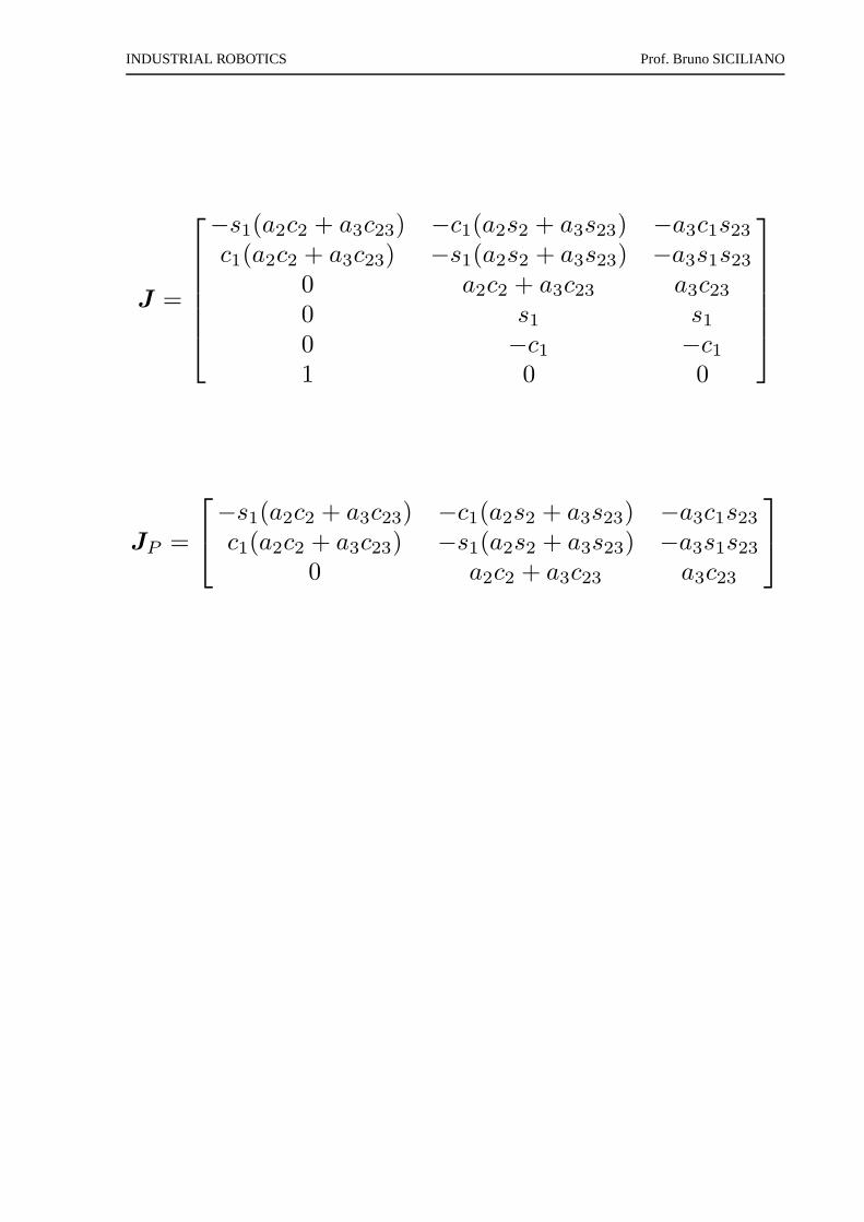
Anthropomorphic arm
INDUSTRIAL ROBOTICS Prof. Bruno SICILIANO
J =
[
z0 × (p − p0) z1 × (p − p1) z2 × (p − p2)z0 z1 z2
]
p0 = p1 =
000
p2 =
a2c1c2a2s1c2a2s2
p =
c1(a2c2 + a3c23)s1(a2c2 + a3c23)a2s2 + a3s23
z0 =
001
z1 = z2 =
s1−c10
INDUSTRIAL ROBOTICS Prof. Bruno SICILIANO
J =
−s1(a2c2 + a3c23) −c1(a2s2 + a3s23) −a3c1s23c1(a2c2 + a3c23) −s1(a2s2 + a3s23) −a3s1s23
0 a2c2 + a3c23 a3c230 s1 s10 −c1 −c11 0 0
JP =
−s1(a2c2 + a3c23) −c1(a2s2 + a3s23) −a3c1s23c1(a2c2 + a3c23) −s1(a2s2 + a3s23) −a3s1s23
0 a2c2 + a3c23 a3c23
INDUSTRIAL ROBOTICS Prof. Bruno SICILIANO
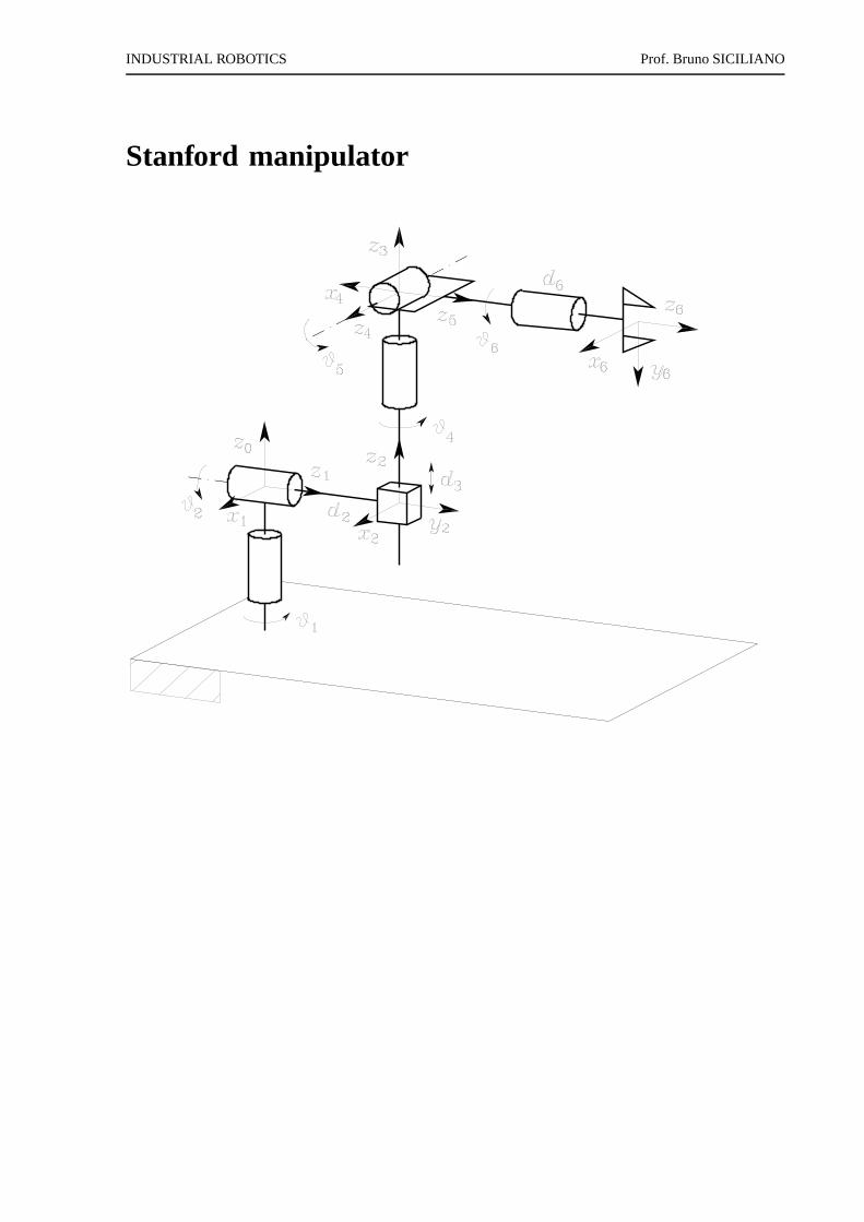
Stanford manipulator
INDUSTRIAL ROBOTICS Prof. Bruno SICILIANO
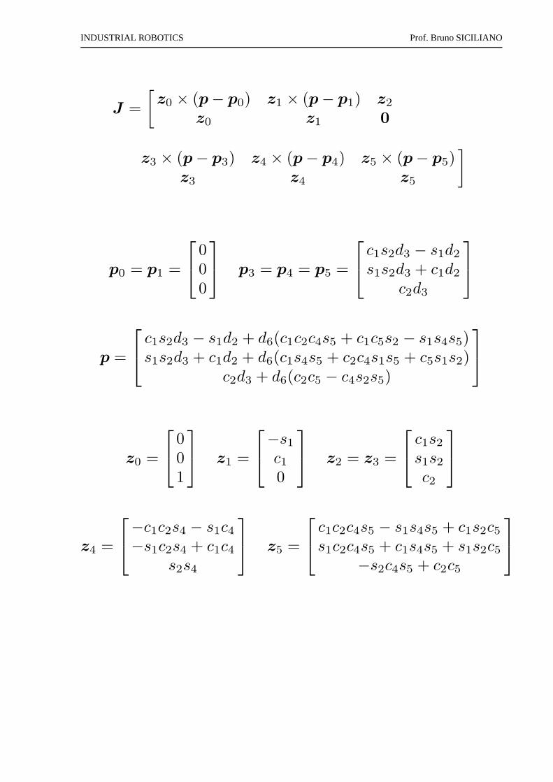
J =
[
z0 × (p − p0) z1 × (p − p1) z2
z0 z1 0
z3 × (p − p3) z4 × (p − p4) z5 × (p − p5)z3 z4 z5
]
p0 = p1 =
000
p3 = p4 = p5 =
c1s2d3 − s1d2
s1s2d3 + c1d2
c2d3
p =
c1s2d3 − s1d2 + d6(c1c2c4s5 + c1c5s2 − s1s4s5)s1s2d3 + c1d2 + d6(c1s4s5 + c2c4s1s5 + c5s1s2)
c2d3 + d6(c2c5 − c4s2s5)
z0 =
001
z1 =
−s1c10
z2 = z3 =
c1s2s1s2c2
z4 =
−c1c2s4 − s1c4−s1c2s4 + c1c4
s2s4
z5 =
c1c2c4s5 − s1s4s5 + c1s2c5s1c2c4s5 + c1s4s5 + s1s2c5
−s2c4s5 + c2c5
INDUSTRIAL ROBOTICS Prof. Bruno SICILIANO
KINEMATIC SINGULARITIES
v = J(q)q
• if J is rank-deficient =⇒ kinematic singularities
(a) reduced mobility
(b) infinite solutions to inverse kinematics problem
(c) large joint velocities (in the neighbourhood of singularity)
• Classification
⋆ Boundarysingularities
⋆ Internalsingularities
INDUSTRIAL ROBOTICS Prof. Bruno SICILIANO
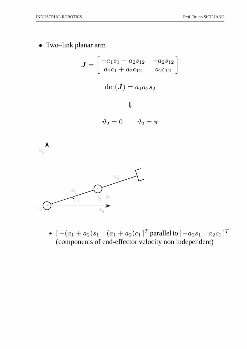
• Two–link planar arm
J =
[
−a1s1 − a2s12 −a2s12a1c1 + a2c12 a2c12
]
det(J) = a1a2s2
⇓
ϑ2 = 0 ϑ2 = π
⋆ [−(a1 + a2)s1 (a1 + a2)c1 ]T parallel to[−a2s1 a2c1 ]T
(components of end-effector velocity non independent)
INDUSTRIAL ROBOTICS Prof. Bruno SICILIANO
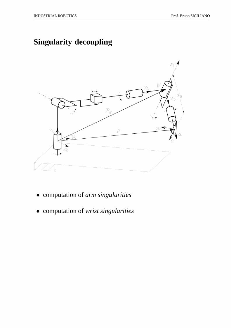
Singularity decoupling
• computation ofarm singularities
• computation ofwrist singularities
INDUSTRIAL ROBOTICS Prof. Bruno SICILIANO
J =
[
J11 J12
J21 J22
]
J12 =[
z3 × (p − p3) z4 × (p − p4) z5 × (p − p5)]
J22 =[
z3 z4 z5
]
• p = pW =⇒ pW − pi parallel tozi, i = 3, 4, 5
J12 =[
0 0 0]
det(J) = det(J11)det(J22)
det(J11) = 0 det(J22) = 0
INDUSTRIAL ROBOTICS Prof. Bruno SICILIANO
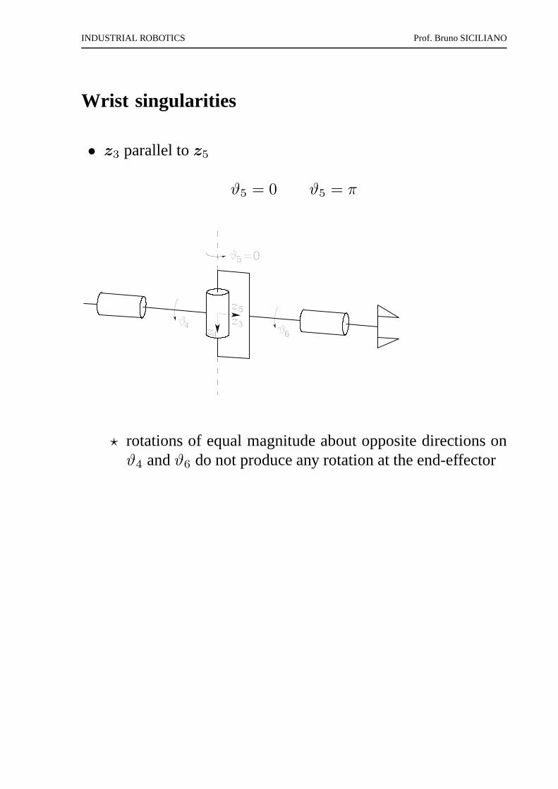
Wrist singularities
• z3 parallel toz5
ϑ5 = 0 ϑ5 = π
⋆ rotations of equal magnitude about opposite directions onϑ4 andϑ6 do not produce any rotation at the end-effector
INDUSTRIAL ROBOTICS Prof. Bruno SICILIANO
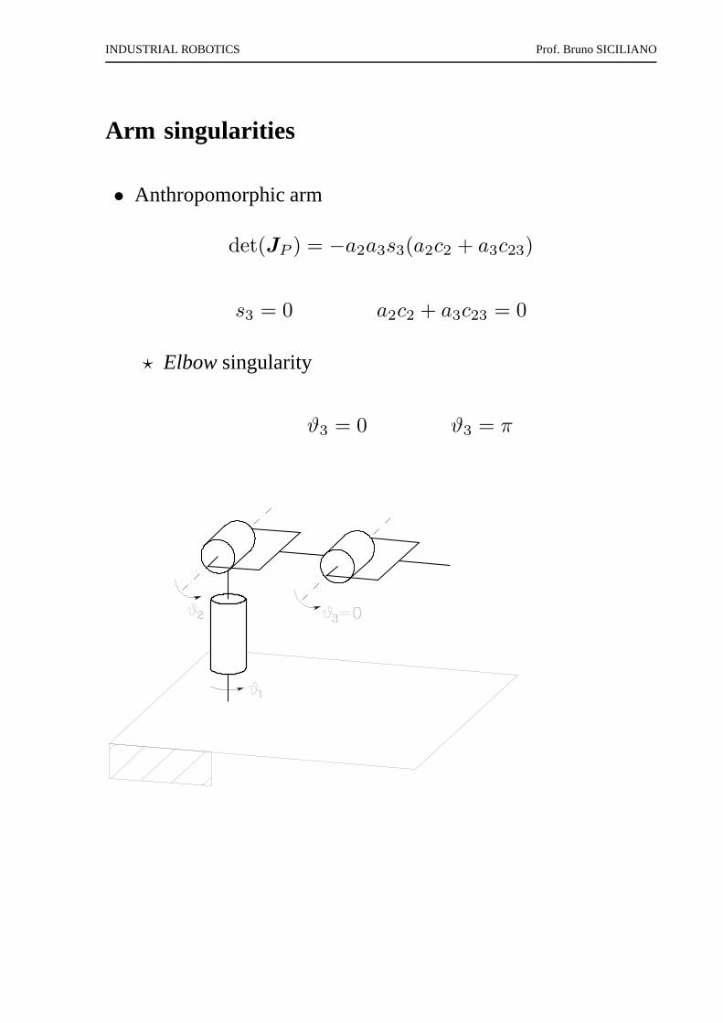
Arm singularities
• Anthropomorphic arm
det(JP ) = −a2a3s3(a2c2 + a3c23)
s3 = 0 a2c2 + a3c23 = 0
⋆ Elbowsingularity
ϑ3 = 0 ϑ3 = π
INDUSTRIAL ROBOTICS Prof. Bruno SICILIANO
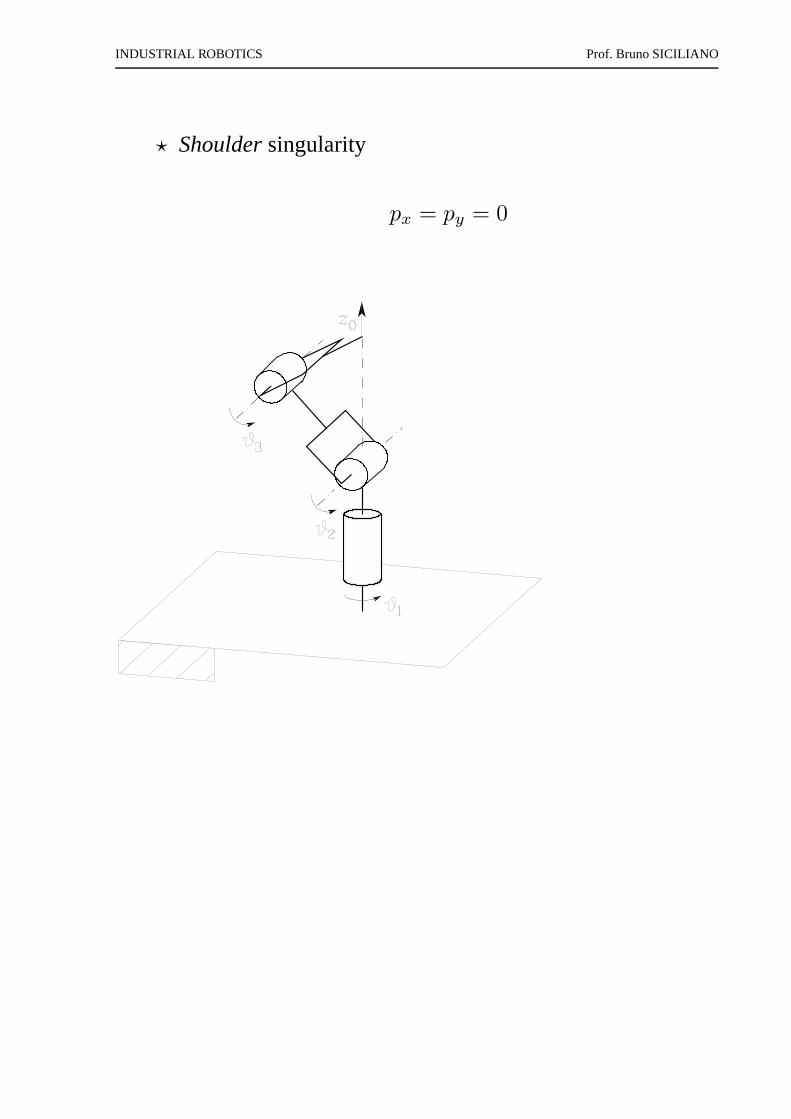
⋆ Shouldersingularity
px = py = 0
INDUSTRIAL ROBOTICS Prof. Bruno SICILIANO
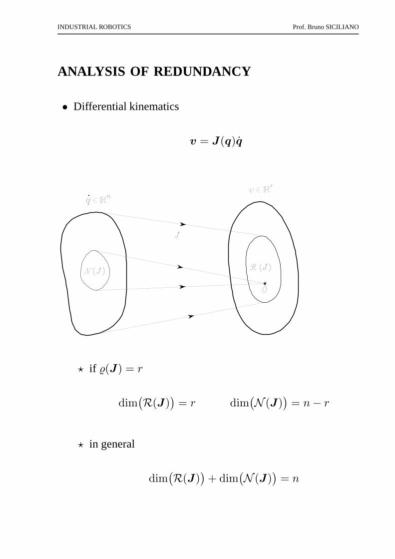
ANALYSIS OF REDUNDANCY
• Differential kinematics
v = J(q)q
⋆ if (J) = r
dim(
R(J))
= r dim(
N (J))
= n− r
⋆ in general
dim(
R(J))
+ dim(
N (J))
= n
INDUSTRIAL ROBOTICS Prof. Bruno SICILIANO
• If N (J) 6= ∅q = q∗ + P qa
whereR(P ) ≡ N (J)
⋆ check:Jq = Jq∗ + JP qa = Jq∗ = v
• qa generatesinternal motionsof the structure
INDUSTRIAL ROBOTICS Prof. Bruno SICILIANO
INVERSE DIFFERENTIAL KINEMATICS
• Nonlinear kinematics equation
• Differential kinematics equation linear in the velocities
• Givenv(t) + initial conditions =⇒ (q(t), q(t))
⋆ if n = rq = J−1(q)v
q(t) =
∫ t
0
q(ς)dς + q(0)
⋆ (Euler) numerical integration
q(tk+1) = q(tk) + q(tk)∆t
INDUSTRIAL ROBOTICS Prof. Bruno SICILIANO
Redundant manipulators
• For a given configurationq, find the solutionsq that satisfy
v = Jq
and minimize
g(q) =1
2qT Wq
⋆ method of Lagrange multipliers
g(q,λ) =1
2qT Wq + λT (v − Jq)
(
∂g
∂q
)T
= 0
(
∂g
∂λ
)T
= 0
⋆ optimal solution
q = W−1JT (JW−1JT )−1v
⋆ if W = I
q = J†v
whereJ† = JT (JJT )−1
is theright pseudo-inverseof J
INDUSTRIAL ROBOTICS Prof. Bruno SICILIANO
• Use of redundancy
g′(q) =1
2(qT − qT
a )(q − qa)
⋆ like above. . .
g′(q,λ) =1
2(qT − qT
a )(q − qa) + λT (v − Jq)
⋆ optimal solution
q = J†v + (I − J†J)qa
INDUSTRIAL ROBOTICS Prof. Bruno SICILIANO
• Characterization of internal motions
qa = ka
(
∂w(q)
∂q
)T
⋆ manipulability measure
w(q) =√
det(
J(q)JT (q))
⋆ distance from mechanical joint limits
w(q) = −1
2n
n∑
i=1
(
qi − qiqiM − qim
)2
⋆ distance from an obstacle
w(q) = minp,o
‖p(q) − o‖
INDUSTRIAL ROBOTICS Prof. Bruno SICILIANO
Kinematic singularities
• The previous solutions hold only whenJ is full-rank
• If J is not full-rank (singularity)
⋆ if v ∈ R(J) =⇒ solution q extracting all linearlyindependent equations (“physically” executable path)
⋆ if v /∈ R(J) =⇒ the system of equations has nosolution (path cannot be executed)
• Inversion in the neighbourhood of singularities
⋆ det(J) small =⇒ q large
⋆ damped least-squares inverse
J⋆ = JT (JJT + k2I)−1
whereq minimizes
g′′(q) = ‖v − Jq‖2 + k2‖q‖2
INDUSTRIAL ROBOTICS Prof. Bruno SICILIANO
ANALYTICAL JACOBIAN
p = p(q)
φ = φ(q)
p =∂p
∂qq = JP (q)q
φ =∂φ
∂qq = Jφ(q)q
x =
[
p
φ
]
=
[
JP (q)
Jφ(q)
]
q
= JA(q)q
JA(q) =∂k(q)
∂q
INDUSTRIAL ROBOTICS Prof. Bruno SICILIANO
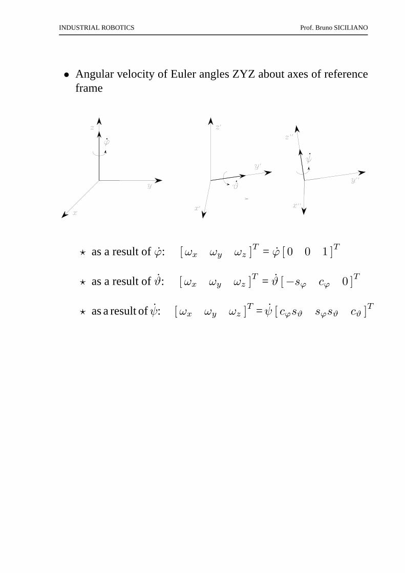
• Angular velocity of Euler angles ZYZ about axes of referenceframe
⋆ as a result ofϕ: [ωx ωy ωz ]T = ϕ [ 0 0 1 ]
T
⋆ as a result ofϑ: [ωx ωy ωz ]T = ϑ [−sϕ cϕ 0 ]
T
⋆ as a result ofψ: [ωx ωy ωz ]T = ψ [ cϕsϑ sϕsϑ cϑ ]
T
INDUSTRIAL ROBOTICS Prof. Bruno SICILIANO
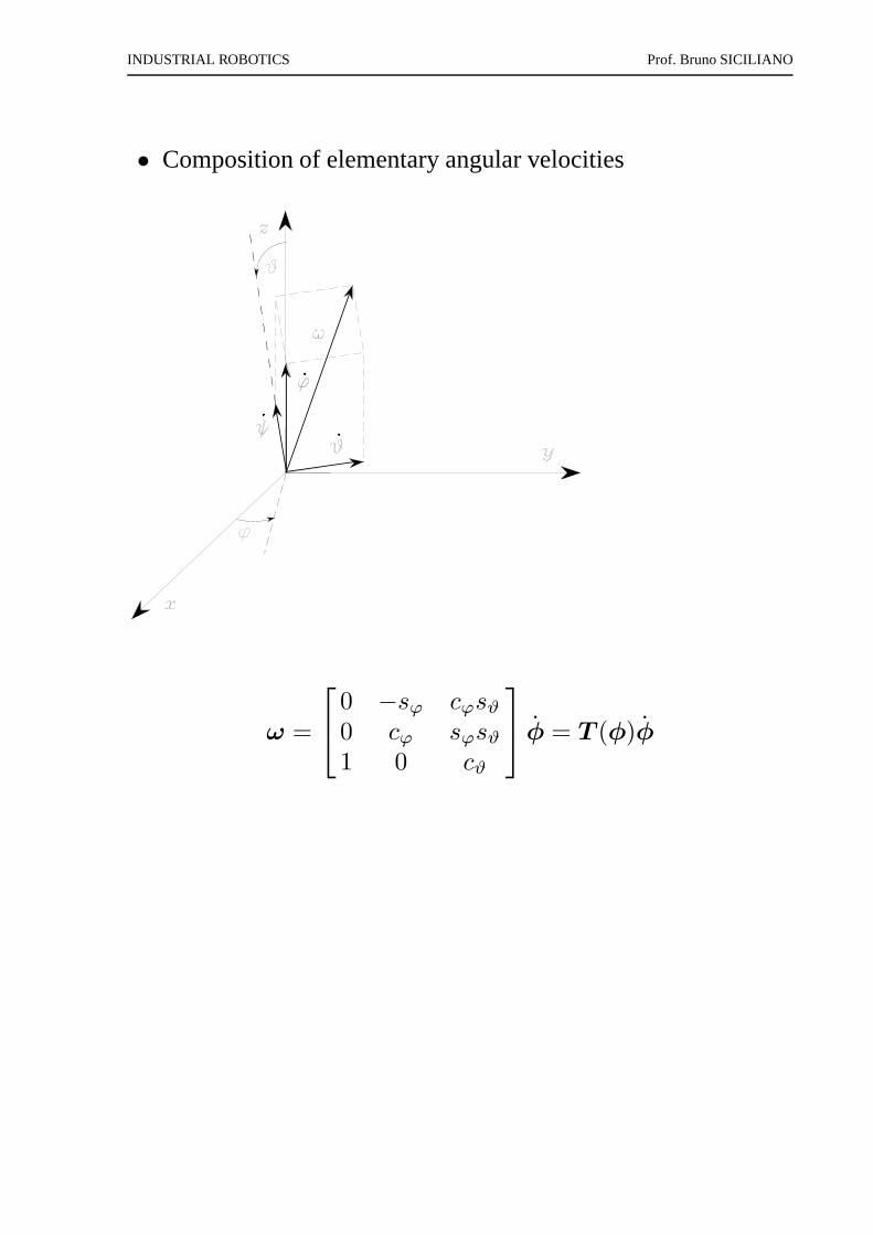
• Composition of elementary angular velocities
ω =
0 −sϕ cϕsϑ
0 cϕ sϕsϑ
1 0 cϑ
φ = T (φ)φ
INDUSTRIAL ROBOTICS Prof. Bruno SICILIANO
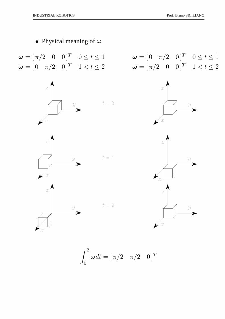
• Physical meaning ofω
ω = [π/2 0 0 ]T 0 ≤ t ≤ 1 ω = [ 0 π/2 0 ]T 0 ≤ t ≤ 1
ω = [ 0 π/2 0 ]T 1 < t ≤ 2 ω = [π/2 0 0 ]T 1 < t ≤ 2
∫ 2
0
ωdt = [π/2 π/2 0 ]T
INDUSTRIAL ROBOTICS Prof. Bruno SICILIANO
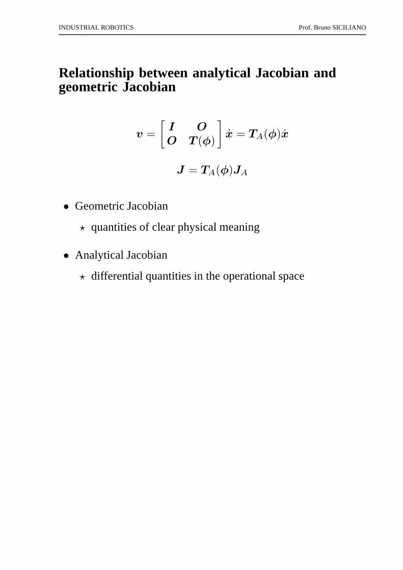
Relationship between analytical Jacobian andgeometric Jacobian
v =
[
I O
O T (φ)
]
x = TA(φ)x
J = TA(φ)JA
• Geometric Jacobian
⋆ quantities of clear physical meaning
• Analytical Jacobian
⋆ differential quantities in the operational space
INDUSTRIAL ROBOTICS Prof. Bruno SICILIANO
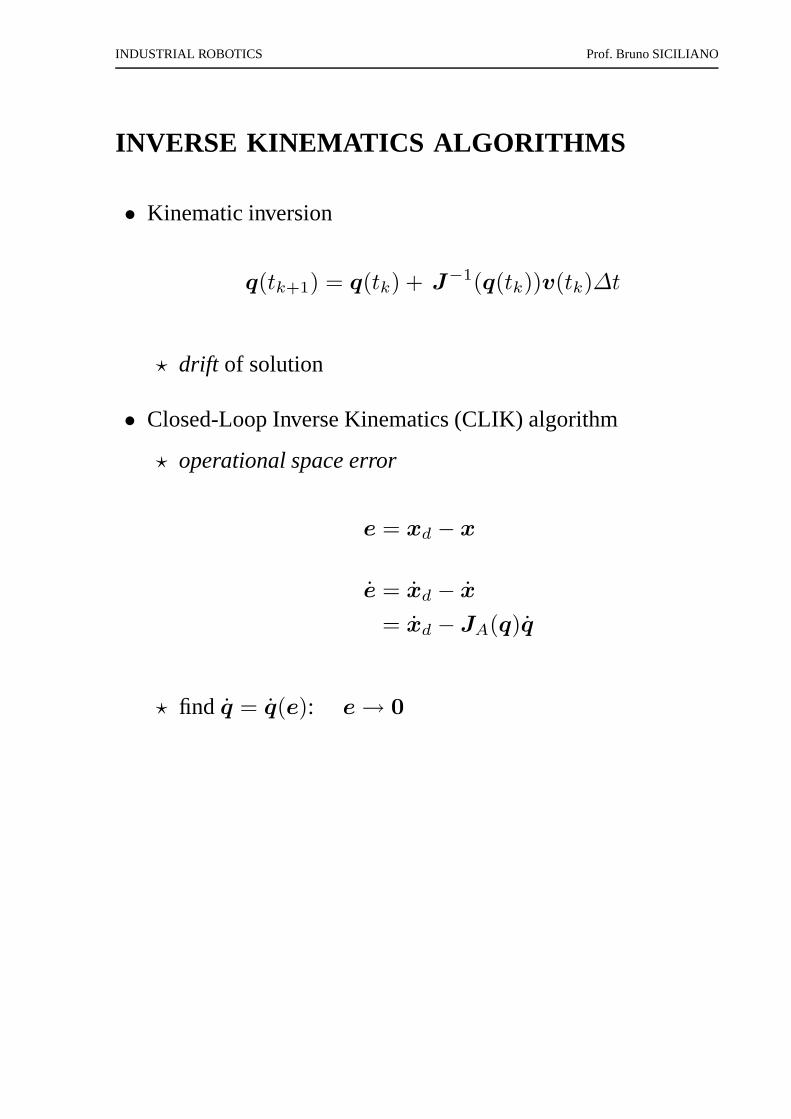
INVERSE KINEMATICS ALGORITHMS
• Kinematic inversion
q(tk+1) = q(tk) + J−1(q(tk))v(tk)∆t
⋆ drift of solution
• Closed-Loop Inverse Kinematics (CLIK) algorithm
⋆ operational space error
e = xd − x
e = xd − x
= xd − JA(q)q
⋆ find q = q(e): e → 0
INDUSTRIAL ROBOTICS Prof. Bruno SICILIANO
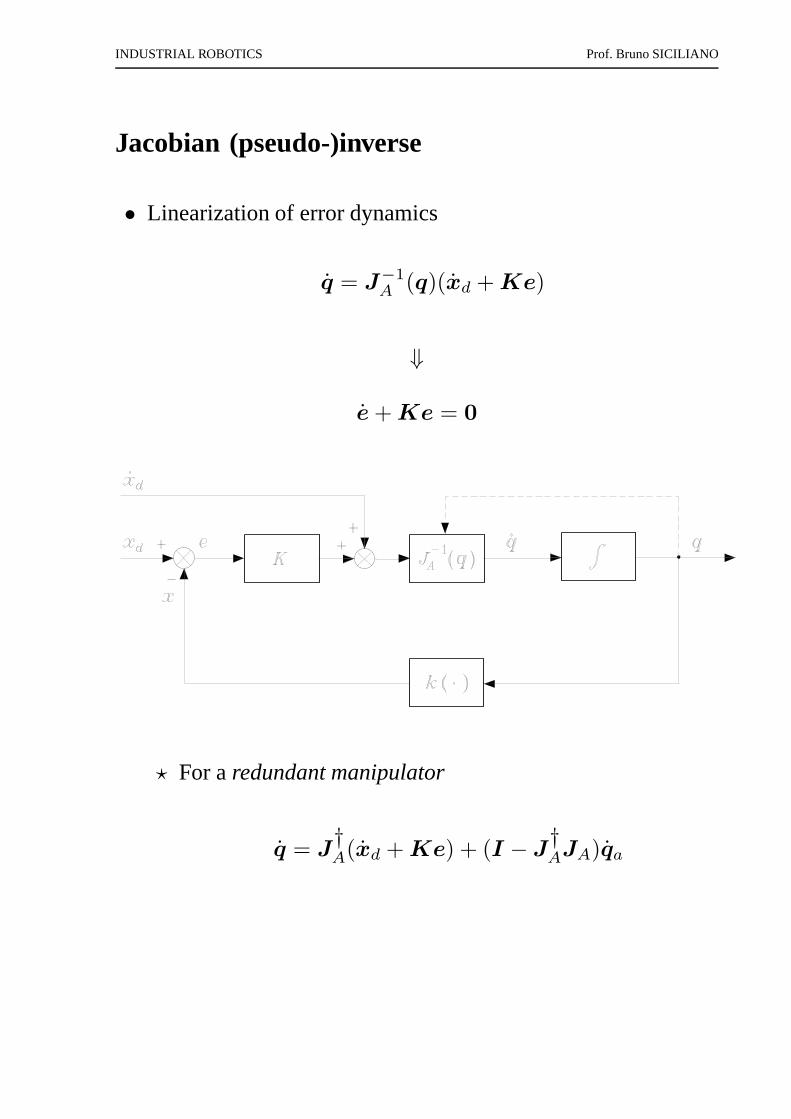
Jacobian (pseudo-)inverse
• Linearization of error dynamics
q = J−1
A (q)(xd + Ke)
⇓
e + Ke = 0
⋆ For aredundant manipulator
q = J†A(xd + Ke) + (I − J
†AJA)qa
INDUSTRIAL ROBOTICS Prof. Bruno SICILIANO
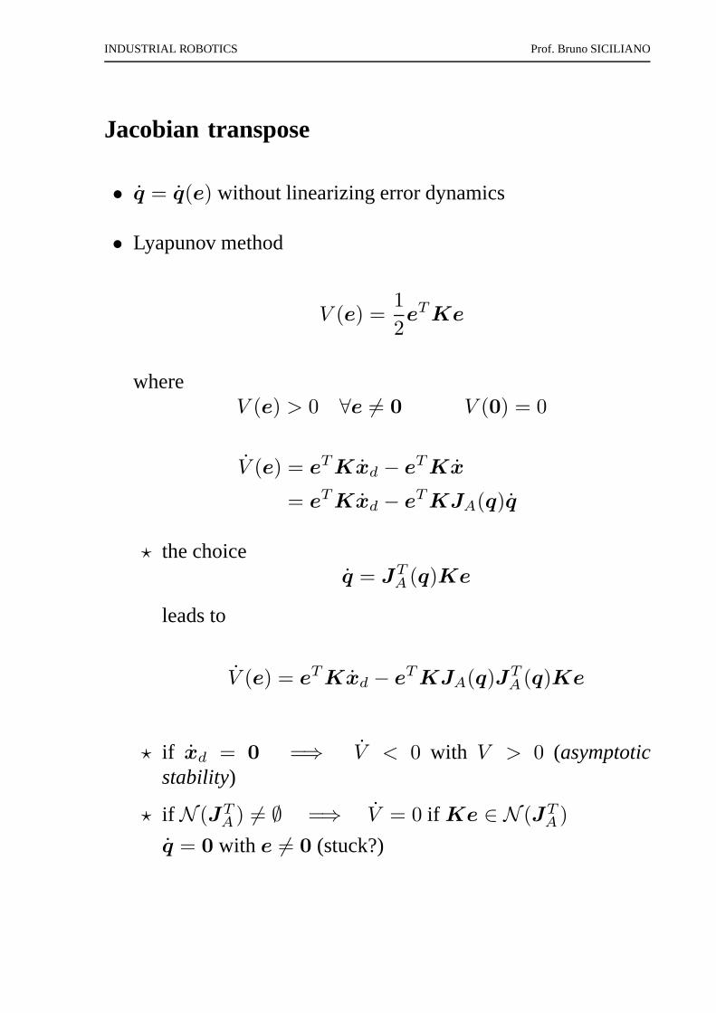
Jacobian transpose
• q = q(e) without linearizing error dynamics
• Lyapunov method
V (e) =1
2eT Ke
whereV (e) > 0 ∀e 6= 0 V (0) = 0
V (e) = eT Kxd − eT Kx
= eT Kxd − eT KJA(q)q
⋆ the choiceq = JT
A (q)Ke
leads to
V (e) = eT Kxd − eT KJA(q)JTA (q)Ke
⋆ if xd = 0 =⇒ V < 0 with V > 0 (asymptoticstability)
⋆ if N (JTA ) 6= ∅ =⇒ V = 0 if Ke ∈ N (JT
A )
q = 0 with e 6= 0 (stuck?)
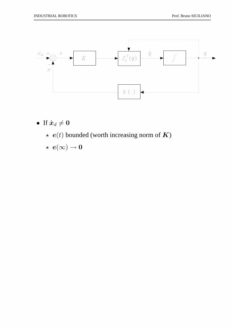
INDUSTRIAL ROBOTICS Prof. Bruno SICILIANO
• If xd 6= 0
⋆ e(t) bounded (worth increasing norm ofK)
⋆ e(∞) → 0
INDUSTRIAL ROBOTICS Prof. Bruno SICILIANO
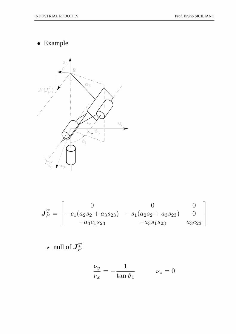
• Example
JTP =
0 0 0−c1(a2s2 + a3s23) −s1(a2s2 + a3s23) 0
−a3c1s23 −a3s1s23 a3c23
⋆ null of JTP
νy
νx= −
1
tanϑ1
νz = 0
INDUSTRIAL ROBOTICS Prof. Bruno SICILIANO
Orientation error
• Position erroreP = pd − p(q)
eP = pd − p
• Euler angleseO = φd − φ(q)
eO = φd − φ
q = J−1
A (q)
[
pd + KP eP
φd + KOeO
]
⋆ handy to assign the time historyφd(t)
⋆ anyhow requires computation ofR = [ n s a ]
• Manipulator with spherical wrist
⋆ computeqP =⇒ RW
⋆ computeRTW Rd =⇒ qO (Euler angles ZYZ)
INDUSTRIAL ROBOTICS Prof. Bruno SICILIANO
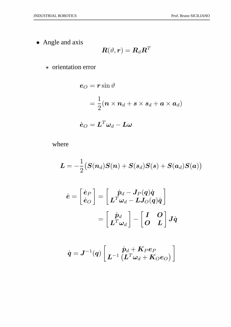
• Angle and axisR(ϑ, r) = RdR
T
⋆ orientation error
eO = r sinϑ
=1
2(n × nd + s × sd + a × ad)
eO = LT ωd − Lω
where
L = −1
2
(
S(nd)S(n) + S(sd)S(s) + S(ad)S(a))
e =
[
eP
eO
]
=
[
pd − JP (q)qLT ωd − LJO(q)q
]
=
[
pd
LT ωd
]
−
[
I O
O L
]
Jq
q = J−1(q)
[
pd + KP eP
L−1(
LT ωd + KOeO
)
]
INDUSTRIAL ROBOTICS Prof. Bruno SICILIANO
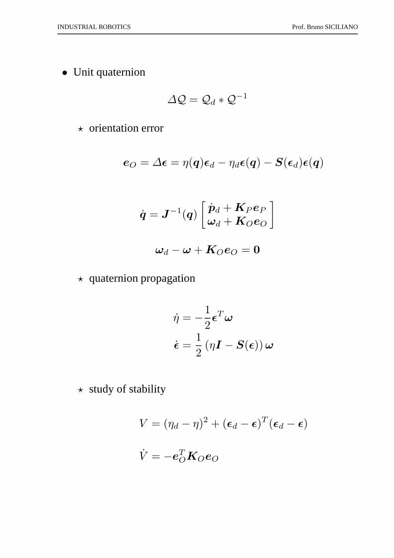
• Unit quaternion
∆Q = Qd ∗ Q−1
⋆ orientation error
eO = ∆ǫ = η(q)ǫd − ηdǫ(q) − S(ǫd)ǫ(q)
q = J−1(q)
[
pd + KP eP
ωd + KOeO
]
ωd − ω + KOeO = 0
⋆ quaternion propagation
η = −1
2ǫT ω
ǫ =1
2(ηI − S(ǫ)) ω
⋆ study of stability
V = (ηd − η)2 + (ǫd − ǫ)T (ǫd − ǫ)
V = −eTOKOeO
INDUSTRIAL ROBOTICS Prof. Bruno SICILIANO
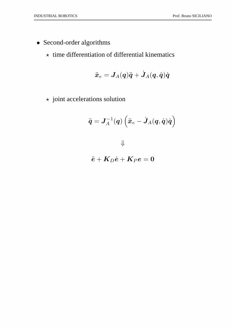
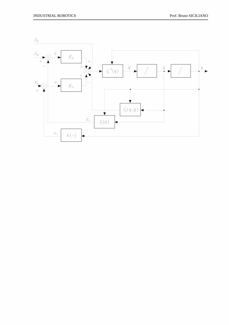
• Second-order algorithms
⋆ time differentiation of differential kinematics
xe = JA(q)q + JA(q, q)q
⋆ joint accelerations solution
q = J−1
A (q)(
xe − JA(q, q)q)
⇓
e + KDe + KP e = 0
INDUSTRIAL ROBOTICS Prof. Bruno SICILIANO
INDUSTRIAL ROBOTICS Prof. Bruno SICILIANO
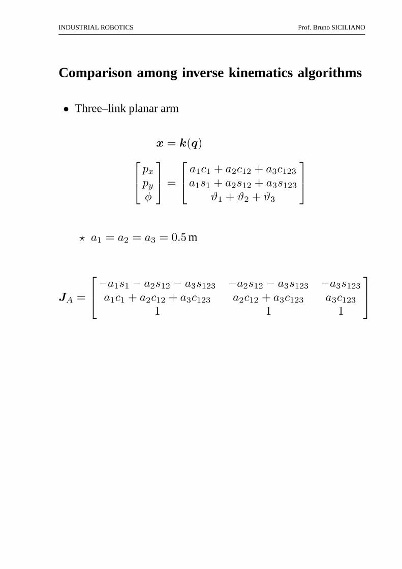
Comparison among inverse kinematics algorithms
• Three–link planar arm
x = k(q)
px
py
φ
=
a1c1 + a2c12 + a3c123a1s1 + a2s12 + a3s123
ϑ1 + ϑ2 + ϑ3
⋆ a1 = a2 = a3 = 0.5 m
JA =
−a1s1 − a2s12 − a3s123 −a2s12 − a3s123 −a3s123a1c1 + a2c12 + a3c123 a2c12 + a3c123 a3c123
1 1 1
INDUSTRIAL ROBOTICS Prof. Bruno SICILIANO
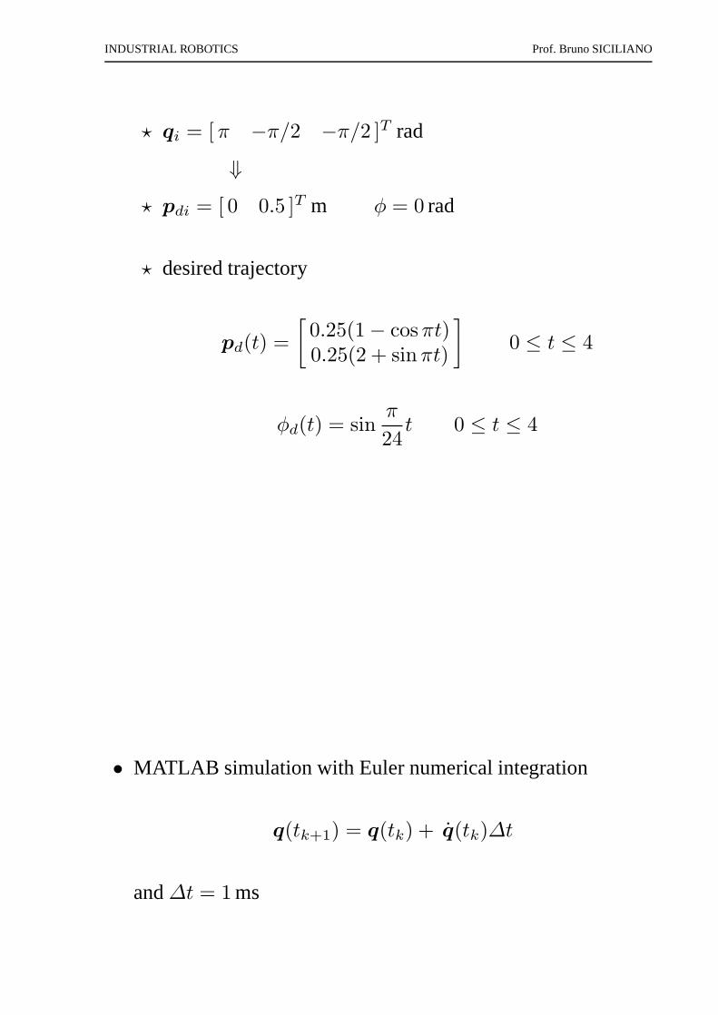
⋆ qi = [π −π/2 −π/2 ]T rad
⇓
⋆ pdi = [ 0 0.5 ]T m φ = 0 rad
⋆ desired trajectory
pd(t) =
[
0.25(1 − cosπt)0.25(2 + sinπt)
]
0 ≤ t ≤ 4
φd(t) = sinπ
24t 0 ≤ t ≤ 4
• MATLAB simulation with Euler numerical integration
q(tk+1) = q(tk) + q(tk)∆t
and∆t = 1 ms
INDUSTRIAL ROBOTICS Prof. Bruno SICILIANO
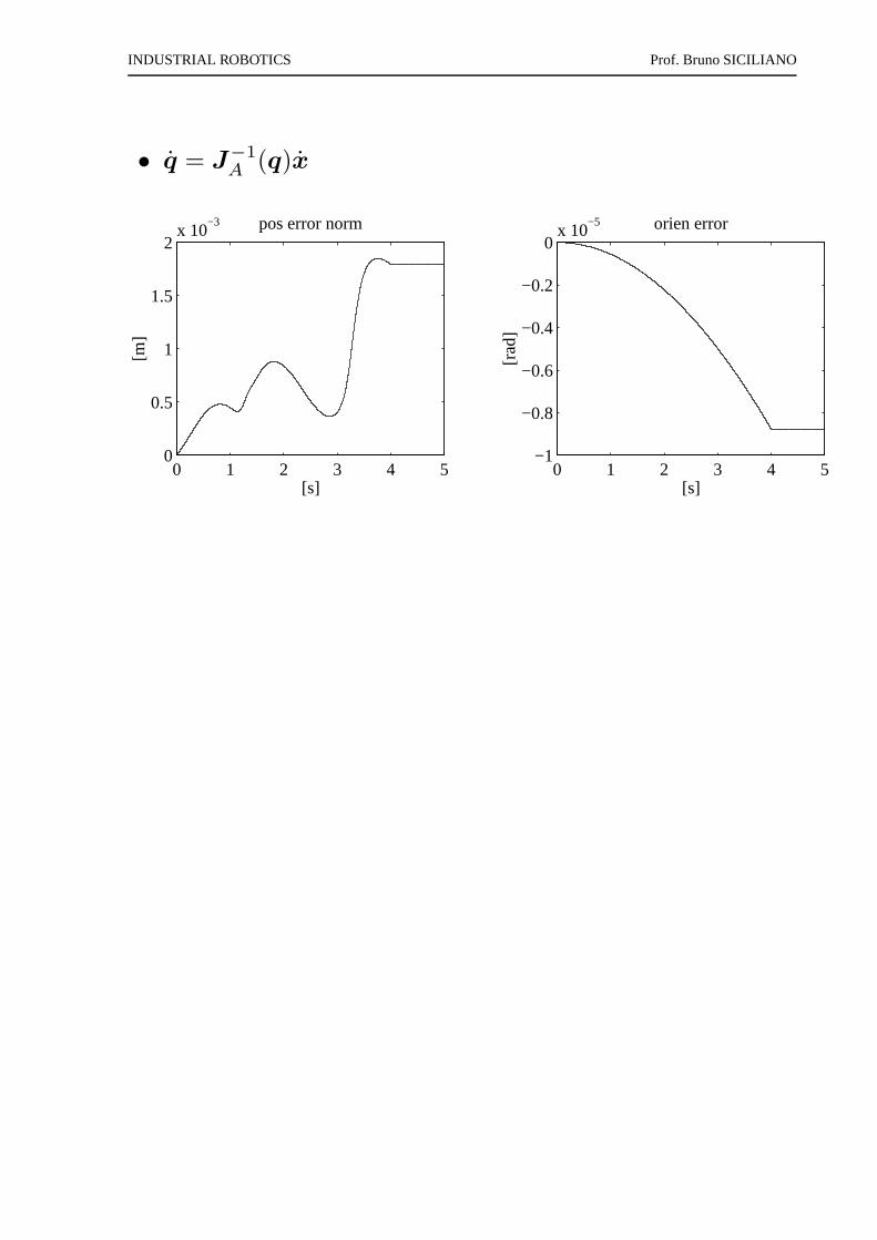
• q = J−1
A (q)x
0 1 2 3 4 50
0.5
1
1.5
2x 10
−3
[s]
[m]
pos error norm
0 1 2 3 4 5−1
−0.8
−0.6
−0.4
−0.2
0x 10
−5
[s][r
ad]
orien error
INDUSTRIAL ROBOTICS Prof. Bruno SICILIANO
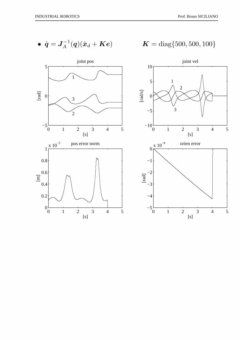
• q = J−1
A (q)(xd + Ke) K = diag{500, 500, 100}
0 1 2 3 4 5−5
0
5
[s]
[rad
]
joint pos
1
2
3
0 1 2 3 4 5−10
−5
0
5
10
[s]
[rad
/s]
joint vel
12
3
0 1 2 3 4 50
0.2
0.4
0.6
0.8
1x 10
−5
[s]
[m]
pos error norm
0 1 2 3 4 5−5
−4
−3
−2
−1
0x 10
−8
[s]
[rad
]orien error
INDUSTRIAL ROBOTICS Prof. Bruno SICILIANO
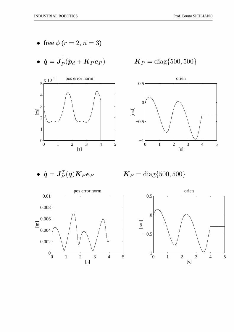
• freeφ (r = 2, n = 3)
• q = J†P (pd + KP eP ) KP = diag{500, 500}
0 1 2 3 4 50
1
2
3
4
5x 10
−6
[s]
[m]
pos error norm
0 1 2 3 4 5−1
−0.5
0
0.5
[s]
[rad
]
orien
• q = JTP (q)KP eP KP = diag{500, 500}
0 1 2 3 4 50
0.002
0.004
0.006
0.008
0.01
[s]
[m]
pos error norm
0 1 2 3 4 5−1
−0.5
0
0.5
[s]
[rad
]
orien
INDUSTRIAL ROBOTICS Prof. Bruno SICILIANO
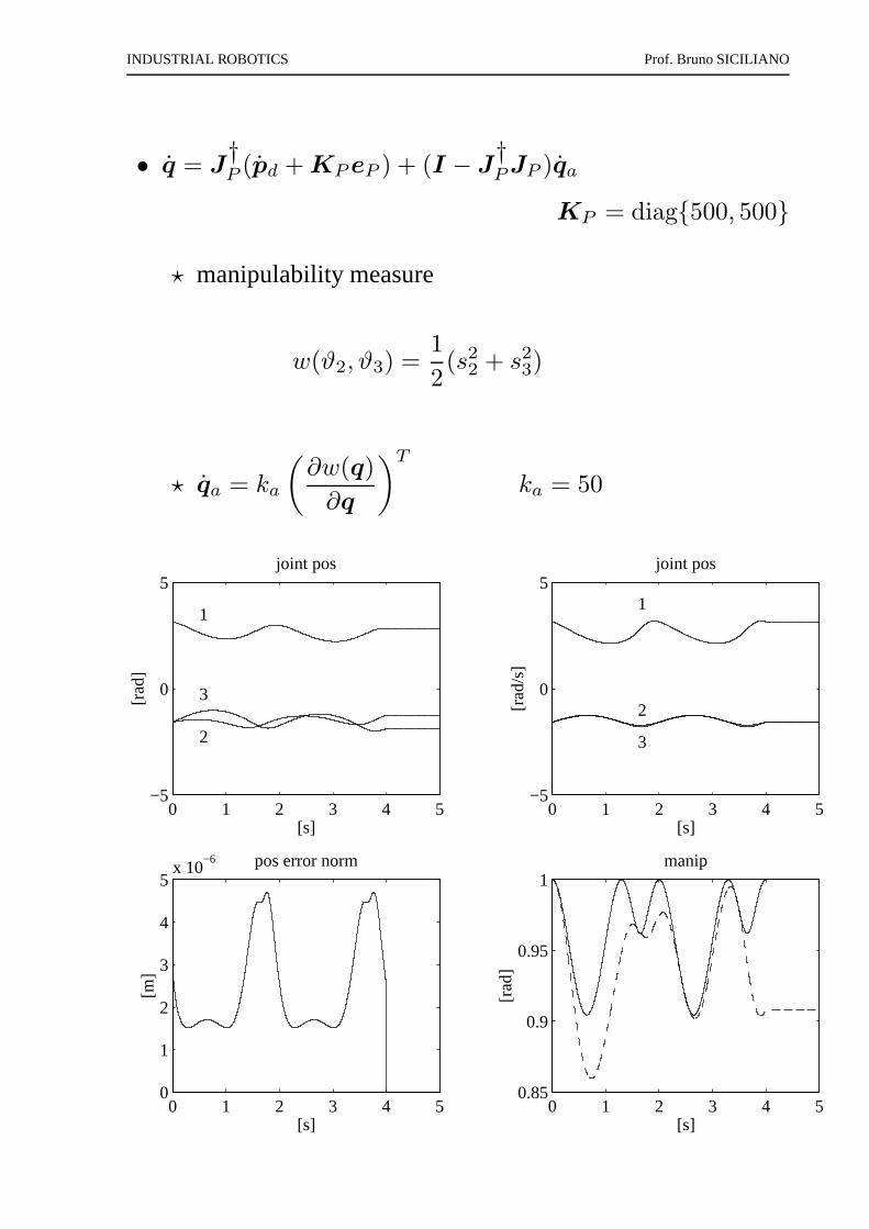
• q = J†P (pd + KP eP ) + (I − J
†P JP )qa
KP = diag{500, 500}
⋆ manipulability measure
w(ϑ2, ϑ3) =1
2(s22 + s23)
⋆ qa = ka
(
∂w(q)
∂q
)T
ka = 50
0 1 2 3 4 5−5
0
5
[s]
[rad
]
joint pos
1
2
3
0 1 2 3 4 5−5
0
5
[s]
[rad
/s]
joint pos
1
2
3
0 1 2 3 4 50
1
2
3
4
5x 10
−6
[s]
[m]
pos error norm
0 1 2 3 4 50.85
0.9
0.95
1
[s]
[rad
]
manip
INDUSTRIAL ROBOTICS Prof. Bruno SICILIANO
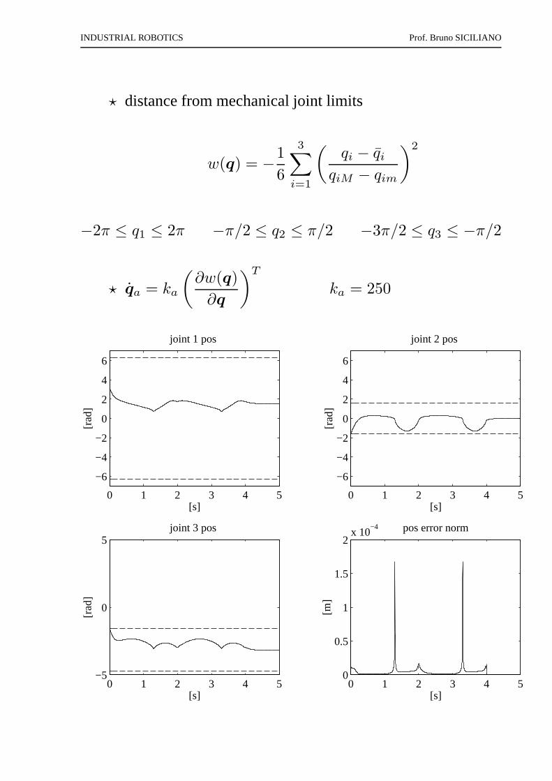
⋆ distance from mechanical joint limits
w(q) = −1
6
3∑
i=1
(
qi − qiqiM − qim
)2
−2π ≤ q1 ≤ 2π −π/2 ≤ q2 ≤ π/2 −3π/2 ≤ q3 ≤ −π/2
⋆ qa = ka
(
∂w(q)
∂q
)T
ka = 250
0 1 2 3 4 50
0.5
1
1.5
2x 10
−4
[s]
[m]
pos error norm
0 1 2 3 4 5
−6
−4
−2
0
2
4
6
[s]
[rad
]
joint 1 pos
0 1 2 3 4 5
−6
−4
−2
0
2
4
6
[s]
[rad
]joint 2 pos
0 1 2 3 4 5−5
0
5
[s]
[rad
]
joint 3 pos
INDUSTRIAL ROBOTICS Prof. Bruno SICILIANO
STATICS
• Relationship between end-effector forces and moments (forces)γ and joint forces and/or torques (torques) τ with manipulatorat equilibrium configuration
⋆ elementary work associated with torques
dWτ = τTdq
⋆ elementary work associated with forces
dWγ = fT dp + µT ωdt
= fT JP (q)dq + µT JO(q)dq
= γT J(q)dq
⋆ elementary displacements≡ virtual displacements
δWτ = τT δq
δWγ = γT J(q)δq
INDUSTRIAL ROBOTICS Prof. Bruno SICILIANO
• Principle of virtual work
⋆ the manipulator is atstatic equilibriumif and only if
δWτ = δWγ ∀δq
⇓
τ = JT (q)γ
INDUSTRIAL ROBOTICS Prof. Bruno SICILIANO
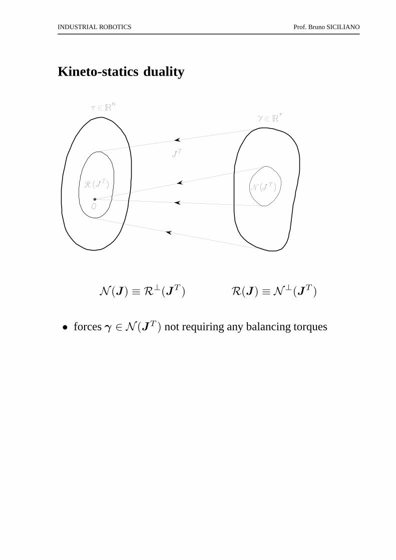
Kineto-statics duality
N (J) ≡ R⊥(JT ) R(J) ≡ N⊥(JT )
• forcesγ ∈ N (JT ) not requiring any balancing torques
INDUSTRIAL ROBOTICS Prof. Bruno SICILIANO
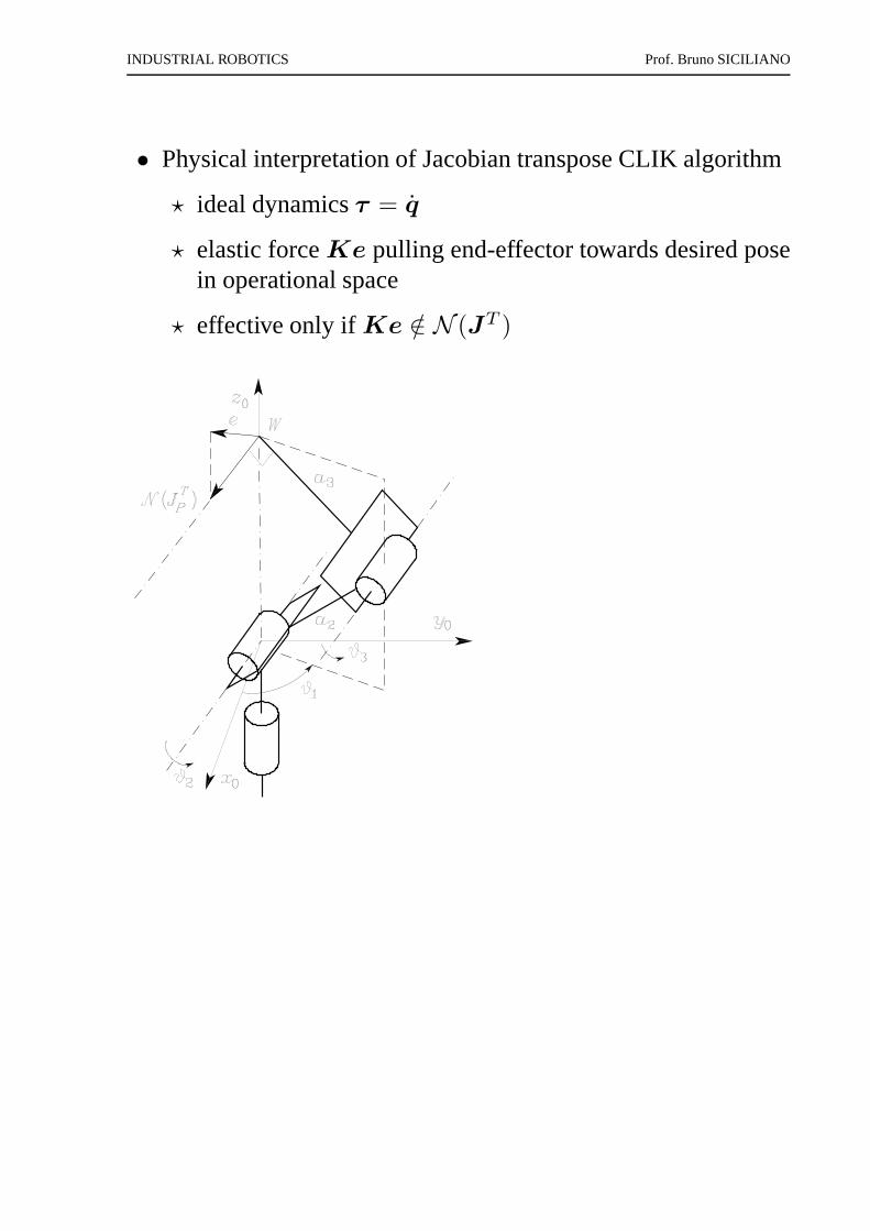
• Physical interpretation of Jacobian transpose CLIK algorithm
⋆ ideal dynamicsτ = q
⋆ elastic forceKe pulling end-effector towards desired posein operational space
⋆ effective only ifKe /∈ N (JT )
INDUSTRIAL ROBOTICS Prof. Bruno SICILIANO
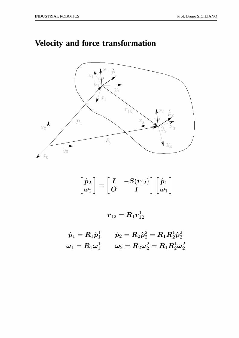
Velocity and force transformation
[
p2
ω2
]
=
[
I −S(r12)O I
] [
p1
ω1
]
r12 = R1r112
p1 = R1p11 p2 = R2p
22 = R1R
12p
22
ω1 = R1ω11 ω2 = R2ω
22 = R1R
12ω
22
INDUSTRIAL ROBOTICS Prof. Bruno SICILIANO
[
p22
ω22
]
=
[
R21 −R2
1S(r112)
O R21
] [
p11
ω11
]
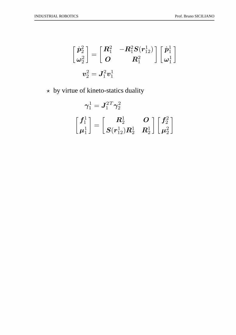
v22 = J2
1 v11
⋆ by virtue of kineto-statics duality
γ11 = J2
1T γ2
2
[
f11
µ11
]
=
[
R12 O
S(r112)R
12 R1
2
] [
f22
µ22
]
INDUSTRIAL ROBOTICS Prof. Bruno SICILIANO
MANIPULABILITY ELLIPSOIDS
• Velocity manipulability ellipsoid
⋆ set of joint velocities of constant (unit) norm
qT q = 1
⋆ redundant manipulator
q = J†(q)v
⇓
vT(
J(q)JT(q))−1
v = 1
• Axes
⋆ eigenvectorsui of JJT =⇒ directions
⋆ singular valuesσi =√
λi(JJT ) =⇒ dimensions
• Volume
⋆ proportional to
w(q) =√
det(
J(q)JT (q))
INDUSTRIAL ROBOTICS Prof. Bruno SICILIANO
Two–link planar arm
• Manipulability measure
w = |det(J)| = a1a2|s2|
⋆ max atϑ2 = ±π/2
⋆ max ata1 = a2 (for given reacha1 + a2)
INDUSTRIAL ROBOTICS Prof. Bruno SICILIANO
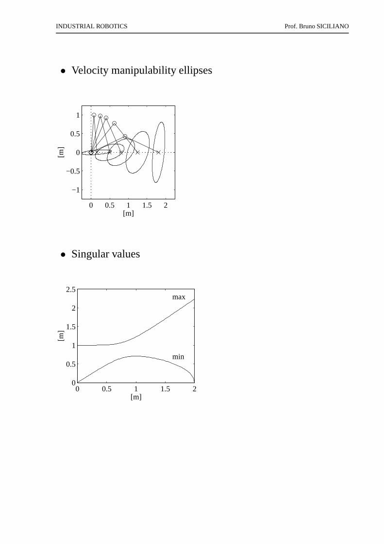
• Velocity manipulability ellipses
0 0.5 1 1.5 2
−1
−0.5
0
0.5
1
[m]
[m]
• Singular values
0 0.5 1 1.5 20
0.5
1
1.5
2
2.5
min
max
[m]
[m]
INDUSTRIAL ROBOTICS Prof. Bruno SICILIANO
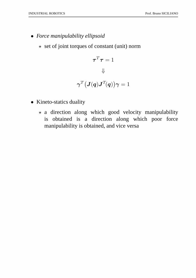
• Force manipulability ellipsoid
⋆ set of joint torques of constant (unit) norm
τT τ = 1
⇓
γT(
J(q)JT(q))
γ = 1
• Kineto-statics duality
⋆ a direction along which good velocity manipulabilityis obtained is a direction along which poor forcemanipulability is obtained, and vice versa
INDUSTRIAL ROBOTICS Prof. Bruno SICILIANO
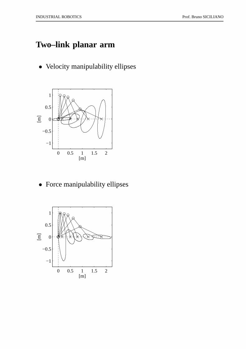
Two–link planar arm
• Velocity manipulability ellipses
0 0.5 1 1.5 2
−1
−0.5
0
0.5
1
[m]
[m]
• Force manipulability ellipses
0 0.5 1 1.5 2
−1
−0.5
0
0.5
1
[m]
[m]
INDUSTRIAL ROBOTICS Prof. Bruno SICILIANO
• Manipulator≡mechanical transformerof velocities and forcesfrom joint space to operational space
⋆ transformation ratio along a direction for force ellipsoid
α(q) =
(
uT J(q)JT (q)u
)−1/2
⋆ transformation ratio along a direction for velocity ellipsoid
β(q) =
(
uT(
J(q)JT (q))−1
u
)−1/2
⋆ use of redundant degrees of freedom
INDUSTRIAL ROBOTICS Prof. Bruno SICILIANO
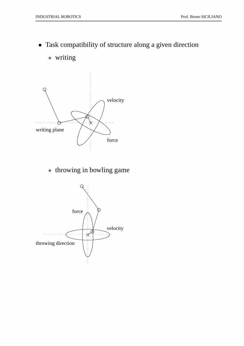
• Task compatibility of structure along a given direction
⋆ writing
force
velocity
writing plane
⋆ throwing in bowling game
force
velocity
throwing direction
Recommended