Genetic Genetic AlgorithmsAlgorithms
Jaap HofstedeBeasly, Bull, Martin
SourcesSources
2
Introduction to Evolutionary Introduction to Evolutionary ComputationComputation
• Evolutionary Computation is the field of study devoted to the design, development, and analysis is problem solvers based on natural selection (simulated evolution).
• Evolution has proven to be a powerful search process.
• Evolutionary Computation has been successfully applied to a wide range of problems including:• Aircraft Design,• Routing in Communications Networks,• Tracking Windshear,• Game Playing (Checkers [Fogel])
3
Introduction to Evolutionary Introduction to Evolutionary ComputationComputation
(Applications cont.)(Applications cont.)• Robotics,• Air Traffic Control,• Design,• Scheduling,• Machine Learning,• Pattern Recognition,• Job Shop Scheduling,• VLSI Circuit Layout,• Strike Force Allocation,

4
Introduction to Evolutionary ComputationIntroduction to Evolutionary Computation(Applications cont.)(Applications cont.)
• Theme Park Tours (Disney Land/World) http://www.TouringPlans.com
• Market Forecasting,• Egg Price Forecasting,• Design of Filters and Barriers,• Data-Mining,• User-Mining,• Resource Allocation,• Path Planning,• Etc.
5
Example of Evolutionary AlgorithmExample of Evolutionary Algorithm
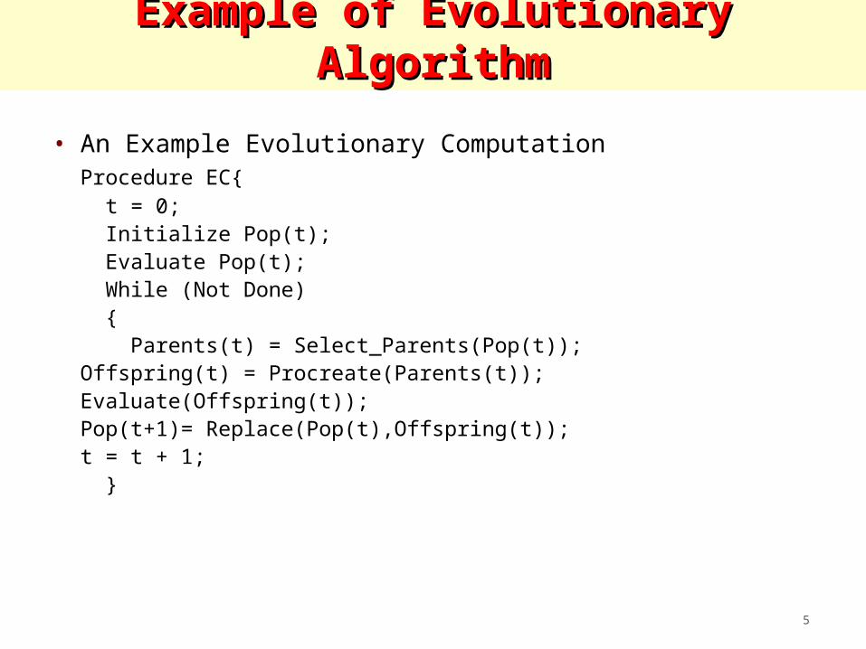
• An Example Evolutionary ComputationProcedure EC{ t = 0; Initialize Pop(t); Evaluate Pop(t); While (Not Done) { Parents(t) = Select_Parents(Pop(t));
Offspring(t) = Procreate(Parents(t));Evaluate(Offspring(t));Pop(t+1)= Replace(Pop(t),Offspring(t));t = t + 1;
}
6
Candidate Solutions CSCandidate Solutions CS
1. In an Evolutionary Computation, a population of candidate solutions (CSs) is randomly generated.
2. Each of the CSs is evaluated and assigned a fitness based on a user specified evaluation function. 1. The evaluation function is used to determine the ‘goodness’ of
a CS.
3. A number of individuals are then selected to be parents based on their fitness.
4. The Select_Parents method must be one that balances the urge for selecting the best performing CSs with the need for population diversity.
7
Parents and GenerationsParents and Generations
1. The selected parents are then allowed to create a set of offspring which are evaluated and assigned a fitness using the same evaluation function defined by the user.
2. Finally, a decision must be made as to which individuals of the current population and the offspring population should be allowed to survive. 1. Typically, in EC , this is done to guarantee that the
population size remains constant.2. [The study of ECs with dynamic population sizes would
make an interesting project for this course]
8
Selecting and StoppingSelecting and Stopping
• Once a decision is made the survivors comprise the next generation (Pop(t+1)).
• This process of selecting parents based on their fitness, allowing them to create offspring, and replacing weaker members of the population is repeated for a user specified number of cycles.
• Stopping conditions for evolutionary search could be:• The discovery of an optimal or near optimal solution• Convergence on a single solution or set of similar solutions,• When the EC detects the problem has no feasible solution,• After a user-specified threshold has been reached, or• After a maximum number of cycles.
9
A Brief History of Evolutionary A Brief History of Evolutionary ComputationComputation
• The idea of using simulated evolution to solve engineering and design problems have been around since the 1950’s (Fogel, 2000).• Bremermann, 1962• Box, 1957• Friedberg, 1958
• However, it wasn’t until the early 1960’s that we began to see three influential forms of EC emerge (Back et al, 1997):• Evolutionary Programming (Lawrence Fogel, 1962),• Genetic Algorithms (Holland, 1962)• Evolution Strategies (Rechenberg, 1965 & Schwefel,
1968),
10
A Brief History of Evolutionary ComputationA Brief History of Evolutionary Computation(cont.)(cont.)
• The designers of each of the EC techniques saw that their particular problems could be solved via simulated evolution.
• Fogel was concerned with solving prediction problems.
• Rechenberg & Schwefel were concerned with solving parameter optimization problems.
• Holland was concerned with developing robust adaptive systems.
11
A Brief History of Evolutionary ComputationA Brief History of Evolutionary Computation(cont.)(cont.)
• Each of these researchers successfully developed appropriate ECs for their particular problems independently.
• In the US, Genetic Algorithms have become the most popular EC technique due to a book by David E. Goldberg (1989) entitled, “Genetic Algorithms in Search, Optimization & Machine Learning”.
• This book explained the concept of Genetic Search in such a way the a wide variety of engineers and scientist could understand and apply.
12
A Brief History of Evolutionary ComputationA Brief History of Evolutionary Computation(cont.)(cont.)
• However, a number of other books helped fuel the growing interest in EC:• Lawrence Davis’, “Handbook of Genetic
Algorithms”, (1991),• Zbigniew Michalewicz’ book (1992), “Genetic
Algorithms + Data Structures = Evolution Programs.
• John R. Koza’s “Genetic Programming” (1992), and • D. B. Fogel’s 1995 book entitled, “Evolutionary
Computation: Toward a New Philosophy of Machine Intelligence.
• These books not only fueled interest in EC but they also were instrumental in bringing together the EP, ES, and GA concepts together in a way that fostered unity and an explosion of new and exciting forms of EC.
13
A Brief History of Evolutionary Computation:A Brief History of Evolutionary Computation:The Evolution of Evolutionary ComputationThe Evolution of Evolutionary Computation
• First Generation EC• EP (Fogel)• GA (Holland)• ES (Rechenberg, Schwefel)
• Second Generation EC• Genetic Evolution of Data Structures (Michalewicz)• Genetic Evolution of Programs (Koza)• Hybrid Genetic Search (Davis)• Tabu Search (Glover)
14
A Brief History of Evolutionary Computation:A Brief History of Evolutionary Computation:The Evolution of Evolutionary Computation (cont.)The Evolution of Evolutionary Computation (cont.)
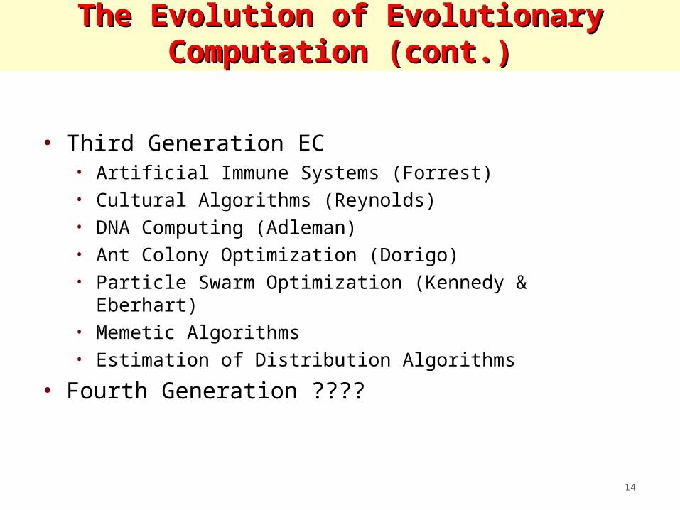
• Third Generation EC• Artificial Immune Systems (Forrest)• Cultural Algorithms (Reynolds)• DNA Computing (Adleman)• Ant Colony Optimization (Dorigo)• Particle Swarm Optimization (Kennedy & Eberhart)• Memetic Algorithms• Estimation of Distribution Algorithms
• Fourth Generation ????
15
Introduction to Evolutionary Introduction to Evolutionary Computation:Computation:
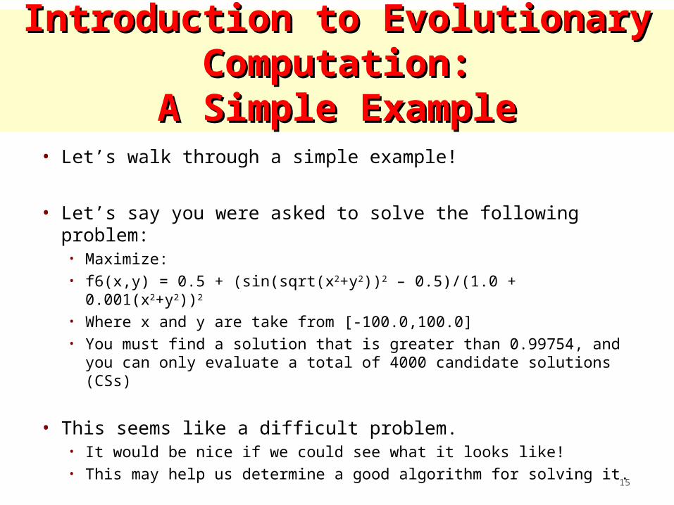
A Simple ExampleA Simple Example• Let’s walk through a simple example!
• Let’s say you were asked to solve the following problem:• Maximize: • f6(x,y) = 0.5 + (sin(sqrt(x2+y2))2 – 0.5)/(1.0 + 0.001(x2+y2))2
• Where x and y are take from [-100.0,100.0]• You must find a solution that is greater than 0.99754, and you
can only evaluate a total of 4000 candidate solutions (CSs)
• This seems like a difficult problem. • It would be nice if we could see what it looks like! • This may help us determine a good algorithm for solving it.
16
Introduction to Evolutionary Computation:Introduction to Evolutionary Computation:A Simple ExampleA Simple Example
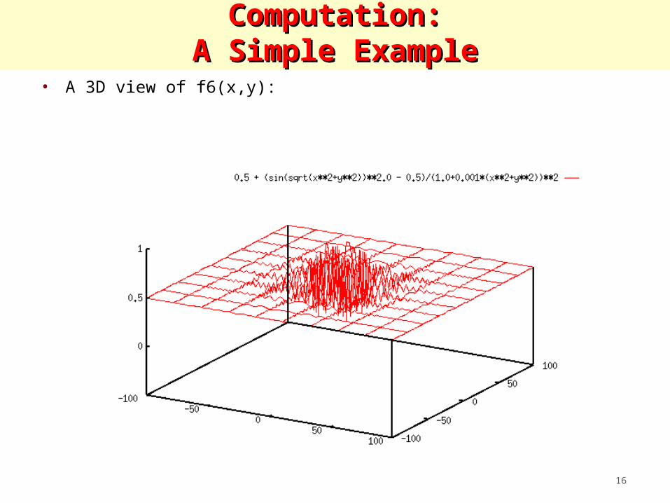
• A 3D view of f6(x,y):
17
Introduction to Evolutionary Computation:Introduction to Evolutionary Computation:A Simple ExampleA Simple Example
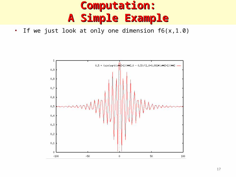
• If we just look at only one dimension f6(x,1.0)
18
Introduction to Evolutionary Computation:Introduction to Evolutionary Computation:A Simple ExampleA Simple Example
• Let’s develop a simple EC for solving this problem
• An individual (chromosome or CS)• <xi,yi>
• fiti = f6(xi,yi)
19
Introduction to Evolutionary Computation:Introduction to Evolutionary Computation:A Simple ExampleA Simple Example
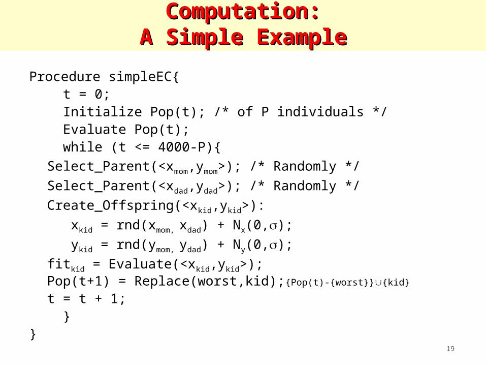
Procedure simpleEC{ t = 0; Initialize Pop(t); /* of P individuals */ Evaluate Pop(t); while (t <= 4000-P){
Select_Parent(<xmom,ymom>); /* Randomly */
Select_Parent(<xdad,ydad>); /* Randomly */
Create_Offspring(<xkid,ykid>):
xkid = rnd(xmom, xdad) + Nx(0,); ykid = rnd(ymom, ydad) + Ny(0,);fitkid = Evaluate(<xkid,ykid>);Pop(t+1) = Replace(worst,kid);{Pop(t)-
{worst}}{kid}
t = t + 1; }
}
20
Introduction to Evolutionary Computation:Introduction to Evolutionary Computation:A Simple ExampleA Simple Example
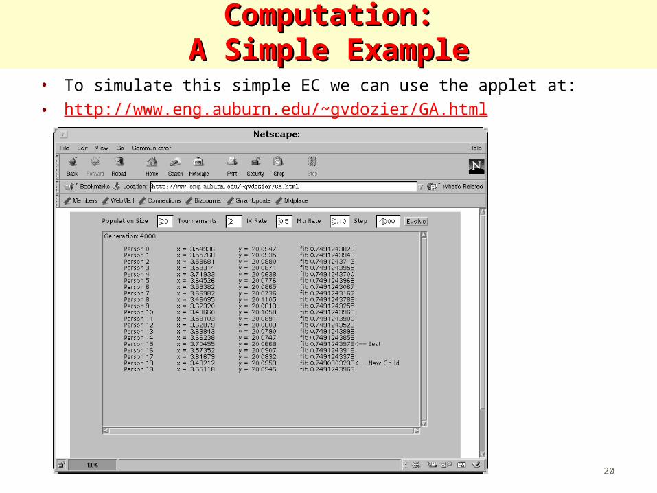
• To simulate this simple EC we can use the applet at:• http://www.eng.auburn.edu/~gvdozier/GA.html
21
Introduction to Evolutionary Computation:Introduction to Evolutionary Computation:A Simple ExampleA Simple Example
• To get a better understanding of some of the properties of ECs let’s do the ‘in class’ lab found at: http://www.eng.auburn.edu/~gvdozier/GA_Lab.html
22
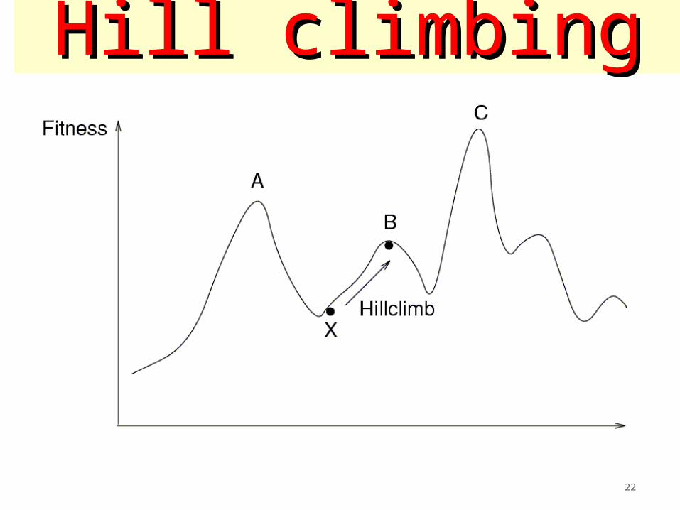
Hill climbingHill climbing
23
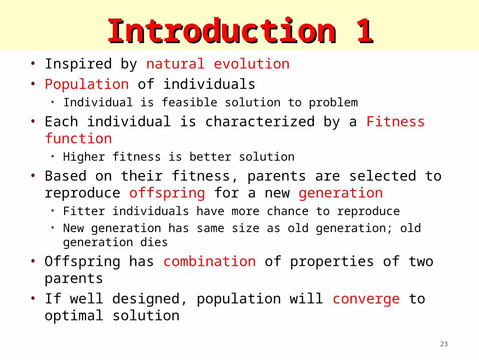
Introduction 1Introduction 1• Inspired by natural evolution• Population of individuals
• Individual is feasible solution to problem
• Each individual is characterized by a Fitness function• Higher fitness is better solution
• Based on their fitness, parents are selected to reproduce offspring for a new generation• Fitter individuals have more chance to reproduce• New generation has same size as old generation; old
generation dies
• Offspring has combination of properties of two parents
• If well designed, population will converge to optimal solution
24
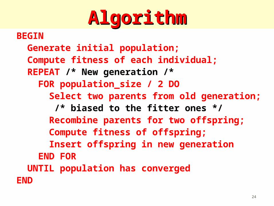
AlgorithmAlgorithmBEGIN Generate initial population; Compute fitness of each individual; REPEAT /* New generation /* FOR population_size / 2 DO Select two parents from old generation; /* biased to the fitter ones */ Recombine parents for two offspring; Compute fitness of offspring; Insert offspring in new generation END FOR UNTIL population has convergedEND
25
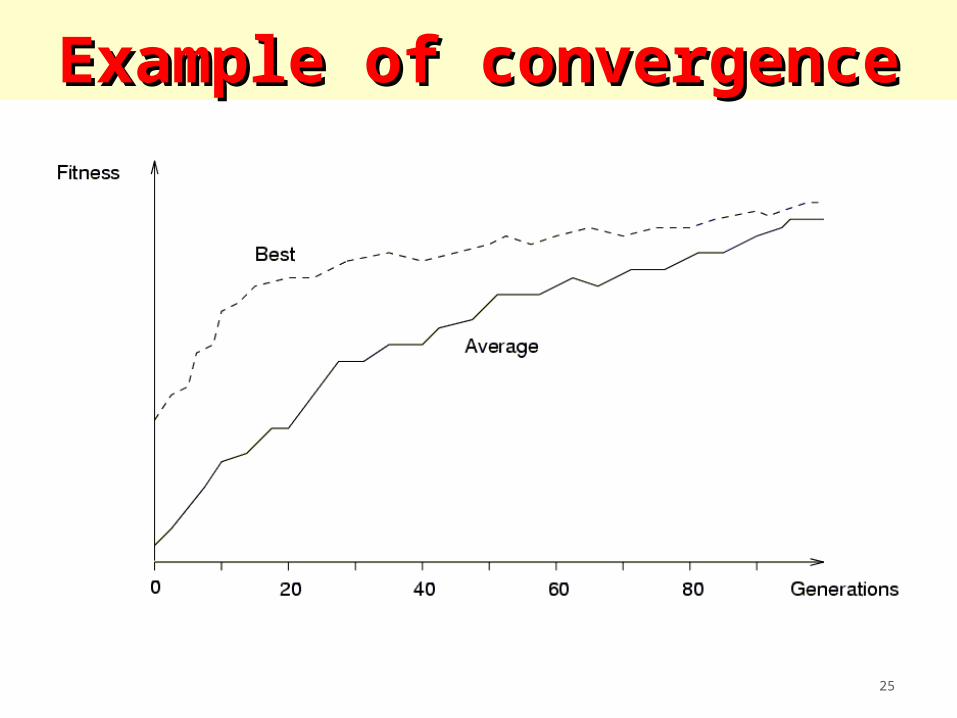
Example of convergenceExample of convergence
26
Introduction 2Introduction 2• Reproduction mechanism has no knowledge of
the problem to be solved
• Link between genetic algorithm and problem:• Coding• Fitness function
27
BasicBasic principles 1principles 1• Coding or Representation
• String with all parameters
• Fitness function• Parent selection
• Reproduction• Crossover• Mutation
• Convergence• When to stop
28
BasicBasic principles 2principles 2• An individual is characterized by a set of
parameters: Genes• The genes are joined into a string: Chromosome
• The chromosome forms the genotype• The genotype contains all information to
construct an organism: the phenotype
• Reproduction is a “dumb” process on the chromosome of the genotype
• Fitness is measured in the real world (‘struggle for life’) of the phenotype
29
CodingCoding• Parameters of the solution (genes) are
concatenated to form a string (chromosome)• All kind of alphabets can be used for a
chromosome (numbers, characters), but generally a binary alphabet is used
• Order of genes on chromosome can be important• Generally many different codings for the
parameters of a solution are possible• Good coding is probably the most important
factor for the performance of a GA• In many cases many possible chromosomes do
not code for feasible solutions
30
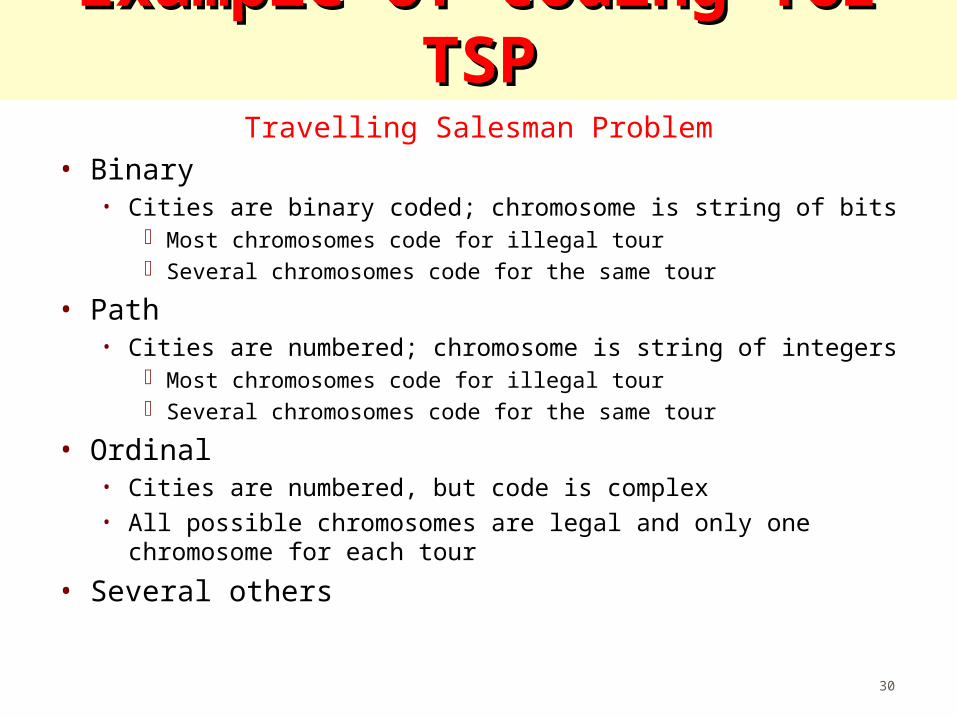
Example of coding for TSPExample of coding for TSPTravelling Salesman Problem
• Binary• Cities are binary coded; chromosome is string of bits
Most chromosomes code for illegal tour Several chromosomes code for the same tour
• Path• Cities are numbered; chromosome is string of integers
Most chromosomes code for illegal tour Several chromosomes code for the same tour
• Ordinal• Cities are numbered, but code is complex• All possible chromosomes are legal and only one
chromosome for each tour
• Several others
31
ReproductionReproduction• Crossover
• Two parents produce two offspring• There is a chance that the chromosomes of the two
parents are copied unmodified as offspring• There is a chance that the chromosomes of the two
parents are randomly recombined (crossover) to form offspring
• Generally the chance of crossover is between 0.6 and 1.0
• Mutation• There is a chance that a gene of a child is changed
randomly• Generally the chance of mutation is low (e.g. 0.001)
32
CrossoverCrossover• One-point crossover• Two-point crossover• Uniform crossover
33
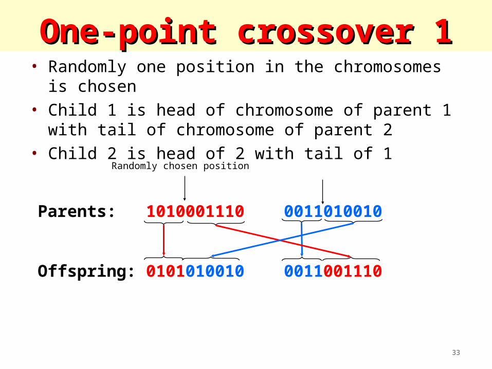
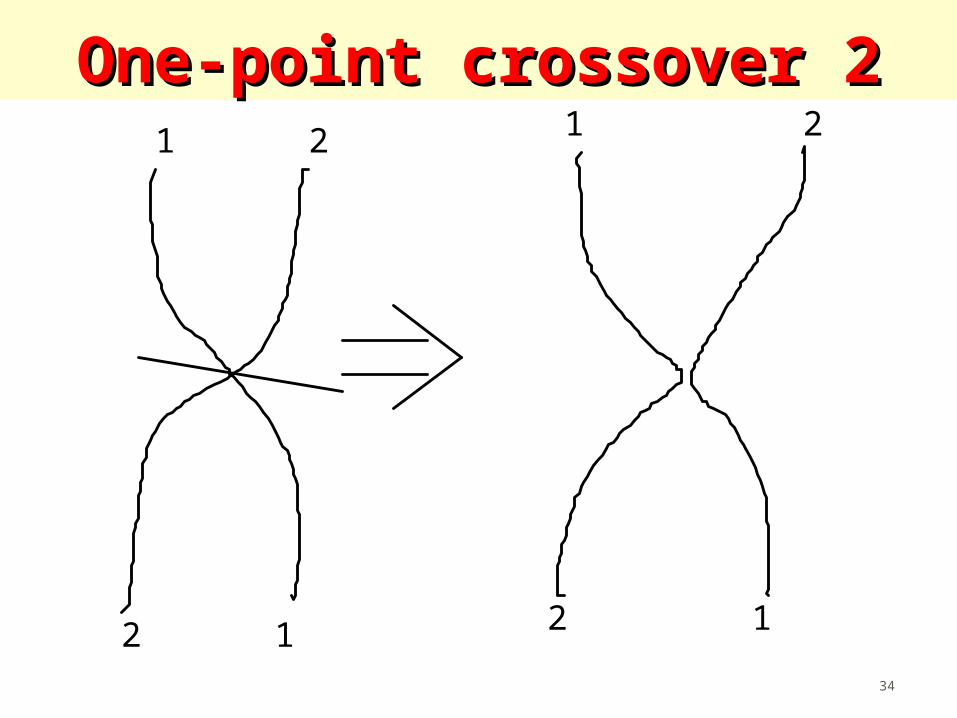
One-point crossover 1One-point crossover 1• Randomly one position in the chromosomes is
chosen• Child 1 is head of chromosome of parent 1 with
tail of chromosome of parent 2• Child 2 is head of 2 with tail of 1
Parents: 1010001110 0011010010
Offspring: 0101010010 0011001110
Randomly chosen position
34
One-point crossover 2One-point crossover 21 2
12
1
2
2
1
35
Two-point crossoverTwo-point crossover
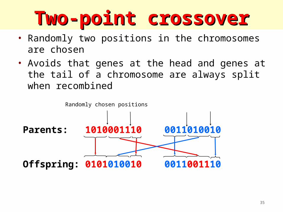
Parents: 1010001110 0011010010
Offspring: 0101010010 0011001110
Randomly chosen positions
• Randomly two positions in the chromosomes are chosen
• Avoids that genes at the head and genes at the tail of a chromosome are always split when recombined
36
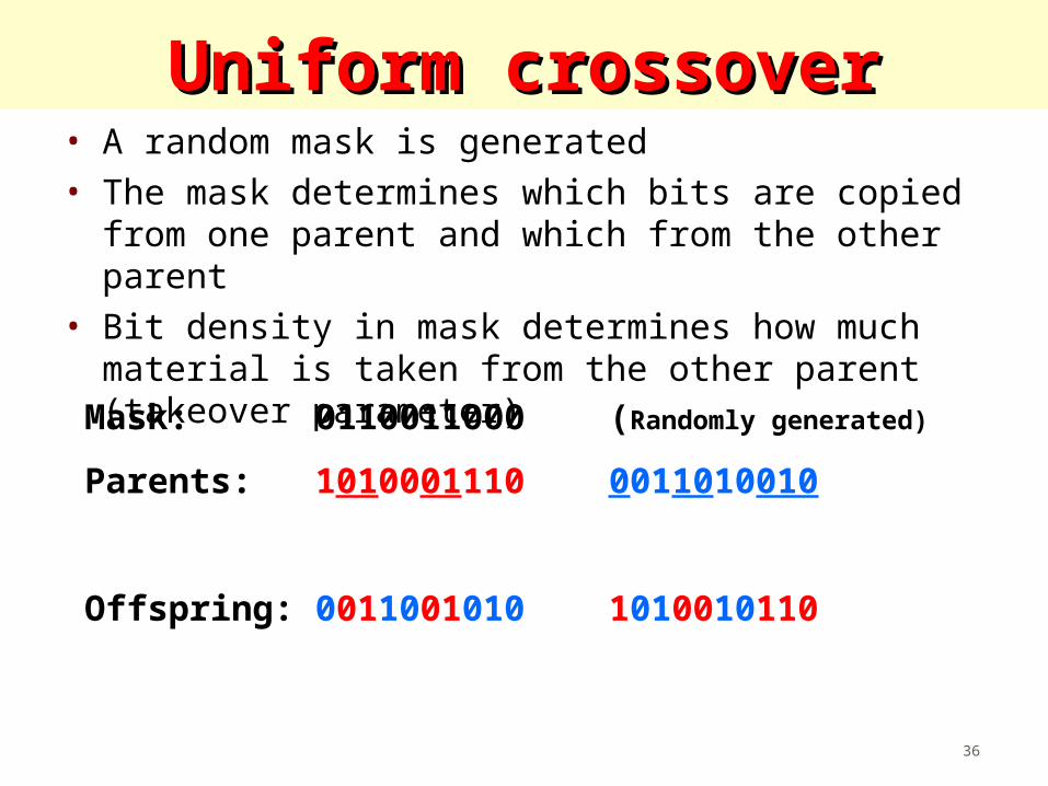
Uniform crossoverUniform crossover• A random mask is generated• The mask determines which bits are copied from
one parent and which from the other parent• Bit density in mask determines how much
material is taken from the other parent (takeover parameter)Mask: 0110011000 (Randomly generated)
Parents: 1010001110 0011010010
Offspring: 0011001010 1010010110
37
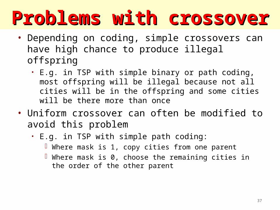
Problems with crossoverProblems with crossover• Depending on coding, simple crossovers can have
high chance to produce illegal offspring• E.g. in TSP with simple binary or path coding, most
offspring will be illegal because not all cities will be in the offspring and some cities will be there more than once
• Uniform crossover can often be modified to avoid this problem• E.g. in TSP with simple path coding:
Where mask is 1, copy cities from one parent Where mask is 0, choose the remaining cities in the order
of the other parent
38
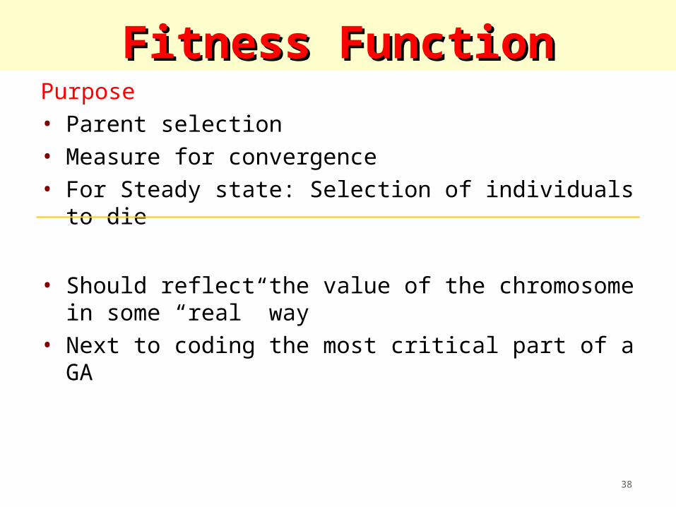
Fitness FunctionFitness FunctionPurpose• Parent selection• Measure for convergence• For Steady state: Selection of individuals to die
• Should reflect the value of the chromosome in some “real” way
• Next to coding the most critical part of a GA
39
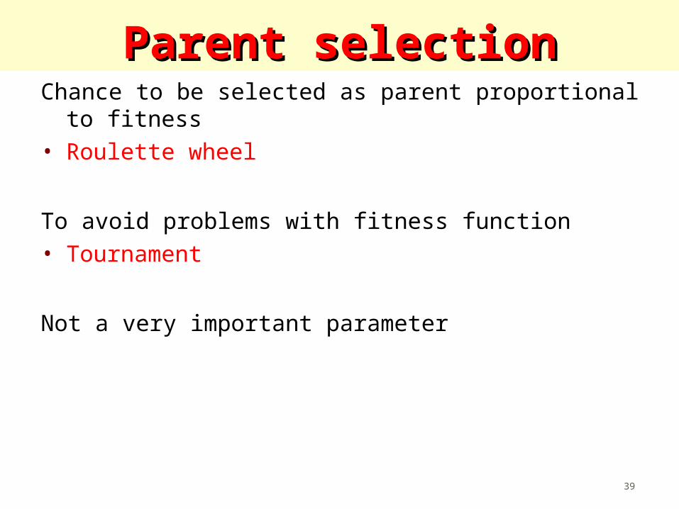
Parent selectionParent selectionChance to be selected as parent proportional to
fitness• Roulette wheel
To avoid problems with fitness function• Tournament
Not a very important parameter
40
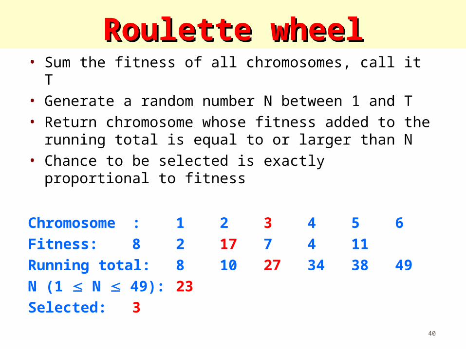
Roulette wheelRoulette wheel• Sum the fitness of all chromosomes, call it T• Generate a random number N between 1 and T• Return chromosome whose fitness added to the
running total is equal to or larger than N• Chance to be selected is exactly proportional to
fitness
Chromosome : 1 2 3 4 5 6
Fitness: 8 2 17 7 4 11
Running total: 8 10 27 34 38 49
N (1 N 49): 23
Selected: 3
41
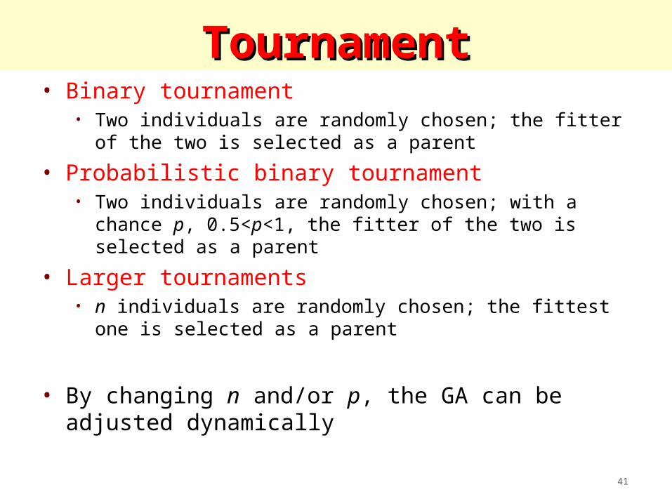
TournamentTournament• Binary tournament
• Two individuals are randomly chosen; the fitter of the two is selected as a parent
• Probabilistic binary tournament• Two individuals are randomly chosen; with a chance p,
0.5<p<1, the fitter of the two is selected as a parent
• Larger tournaments• n individuals are randomly chosen; the fittest one is
selected as a parent
• By changing n and/or p, the GA can be adjusted dynamically
42
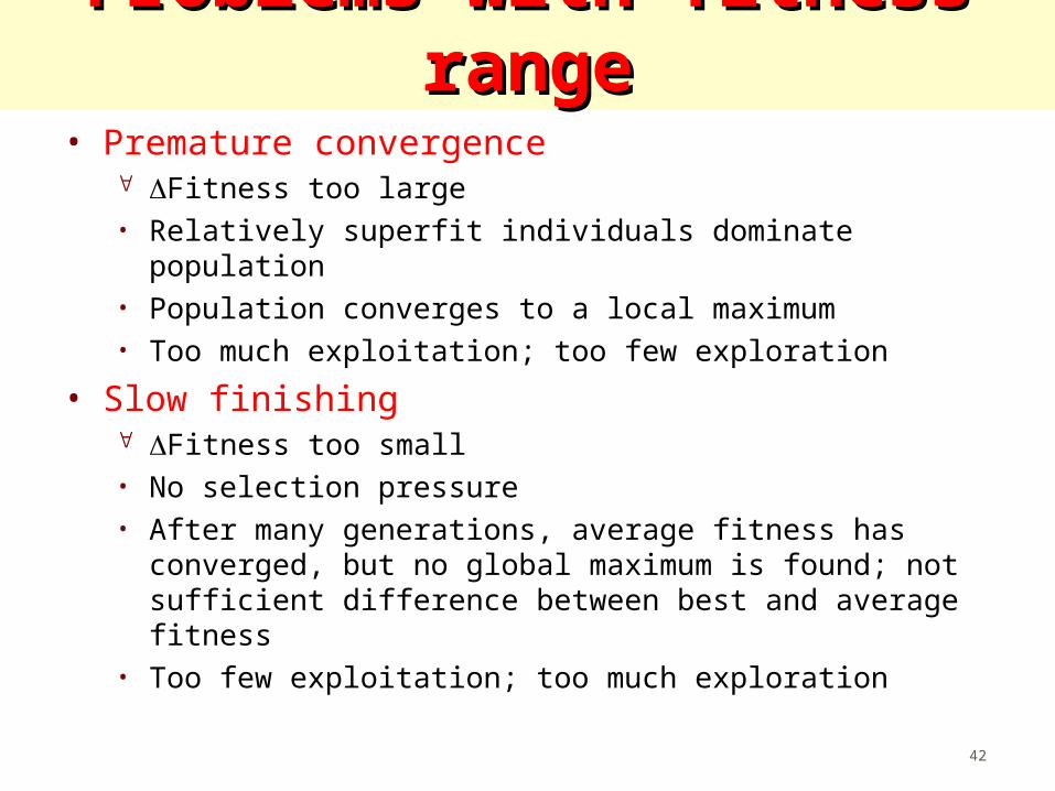
Problems with fitness rangeProblems with fitness range• Premature convergence
Fitness too large• Relatively superfit individuals dominate population• Population converges to a local maximum• Too much exploitation; too few exploration
• Slow finishing Fitness too small• No selection pressure• After many generations, average fitness has converged,
but no global maximum is found; not sufficient difference between best and average fitness
• Too few exploitation; too much exploration
43
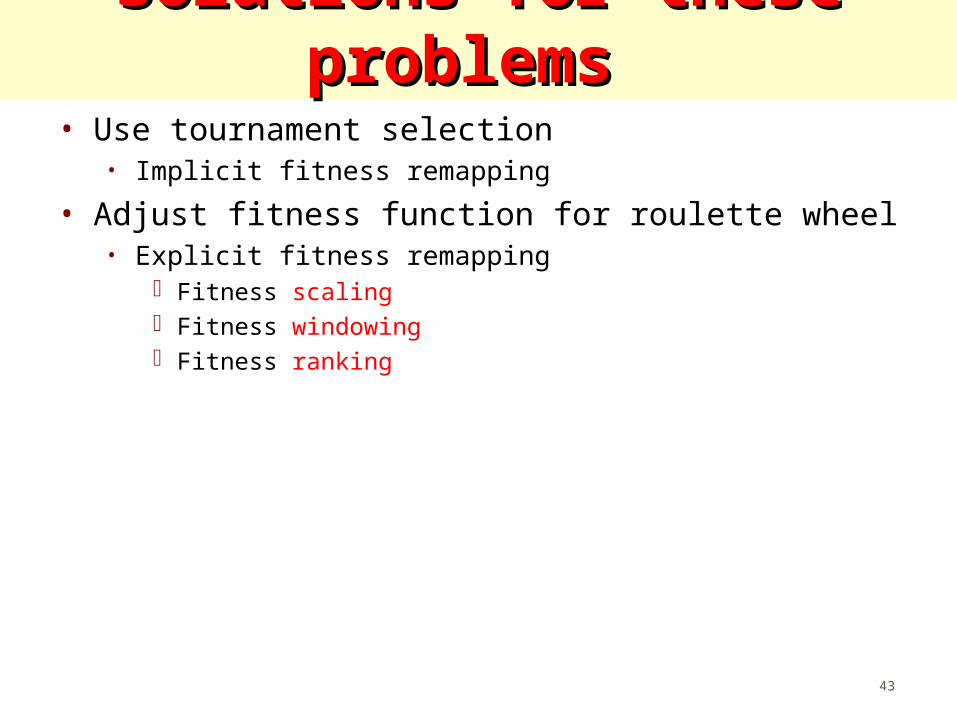
Solutions for these problems Solutions for these problems • Use tournament selection
• Implicit fitness remapping
• Adjust fitness function for roulette wheel• Explicit fitness remapping
Fitness scaling Fitness windowing Fitness ranking
44
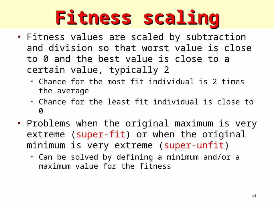
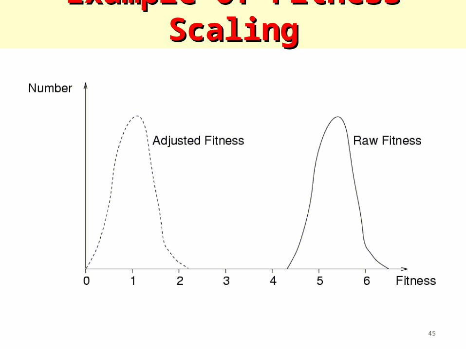
Fitness scalingFitness scaling• Fitness values are scaled by subtraction and
division so that worst value is close to 0 and the best value is close to a certain value, typically 2• Chance for the most fit individual is 2 times the average• Chance for the least fit individual is close to 0
• Problems when the original maximum is very extreme (super-fit) or when the original minimum is very extreme (super-unfit)• Can be solved by defining a minimum and/or a
maximum value for the fitness
45
Example of Fitness ScalingExample of Fitness Scaling
46
Fitness windowingFitness windowing• Same as window scaling, except the amount
subtracted is the minimum observed in the n previous generations, with n e.g. 10
• Same problems as with scaling
47
Fitness rankingFitness ranking• Individuals are numbered in order of increasing
fitness• The rank in this order is the adjusted fitness• Starting number and increment can be chosen in
several ways and influence the results
• No problems with super-fit or super-unfit• Often superior to scaling and windowing
48
Other parameters of GA 1Other parameters of GA 1• Initialization:
• Population size• Random• Dedicated greedy algorithm
• Reproduction: • Generational: as described before (insects)• Generational with elitism: fixed number of most fit
individuals are copied unmodified into new generation• Steady state: two parents are selected to reproduce and
two parents are selected to die; two offspring are immediately inserted in the pool (mammals)
49
Other parameters of GA 2Other parameters of GA 2• Stop criterion:
• Number of new chromosomes• Number of new and unique chromosomes• Number of generations
• Measure:• Best of population• Average of population
• Duplicates• Accept all duplicates• Avoid too many duplicates, because that degenerates
the population (inteelt)• No duplicates at all
50
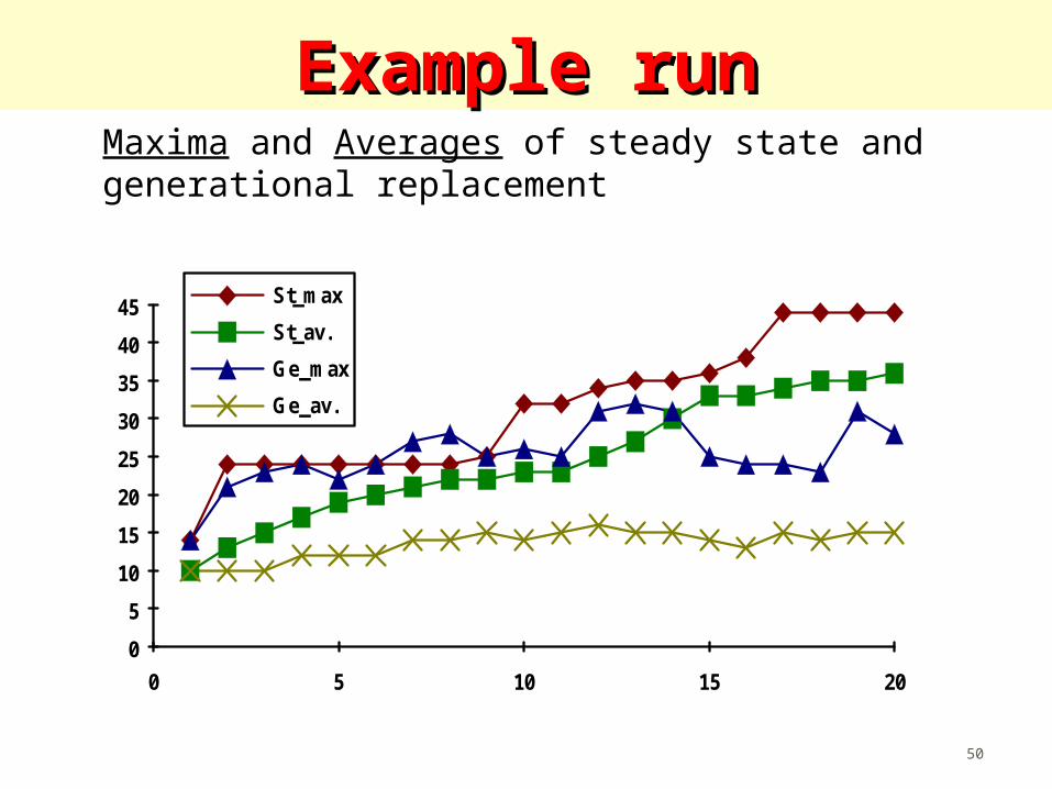
Example runExample runMaxima and Averages of steady state and generational replacement
0
5
10
15
20
25
30
35
40
45
0 5 10 15 20
St_max
St_av.
Ge_max
Ge_av.
51
Introduction to Evolutionary Computation:Introduction to Evolutionary Computation:Reading ListReading List
1. Bäck, T., Hammel, U., and Schwefel, H.-P. (1997). “Evolutionary Computation: Comments on the History and Current State,” IEEE Transactions on Evolutionary Computation, VOL. 1, NO. 1, April 1997.
2. Spears, W. M., De Jong, K. A., Bäck, T., Fogel, D. B., and de Garis, H. (1993). “An Overview of Evolutionary Computation,” The Proceedings of the European Conference on Machine Learning, v667, pp. 442-459. (http://www.cs.uwyo.edu/~wspears/papers/ecml93.pdf)
3. De Jong, Kenneth A., and William M. Spears (1993). “On the State of Evolutionary Computation”, The Proceedings of the Int'l Conference on Genetic Algorithms, pp. 618-623. (http://www.cs.uwyo.edu/~wspears/papers/icga93.pdf)
Recommended