GENERALIZED DAUBECHIES WAVELETSAND APPLICATIONS TO IMAGE
PROCESSING
Hermann RenderUniversity College Dublin (Ireland)
Joint work withOgnyan Kounchev (Bulgarian Academy of Sciences)
Nira Dyn (Tel-Aviv University)David Levin (Tel-Aviv University)
University College Dublin
Overview
Mathematical tools in Signal processing and Image Processing
Daubechies wavelets and Multiresolutional Analysis
Subdivision schemes
Polyharmonic subdivision schemes
Generalized Daubechies wavelets
Regularity of Generalized Daubechies wavelets
University College Dublin

Mathematical tools in Signal and Image Processing
A signal is represented by a function f : R→ R of onevariable x (being square integrable).
An image is presented by a function f : R× R→ R of twovariables. Image processing is much more complex than signalprocessing.
A classical way to process periodic signals is to compute theFourier series
f (x) = a0 + a1 cos x + b1 sin x + a2 cos 2x + b2 sin 2x + ....
Processing the Fourier coefficients an and bn is much easierthan all function values f (x) .
Expanding a function according to suitable basis functions(like cos kx and sin kx for k ∈ Z) simplifies the way ofprocessing data.
University College Dublin
Mathematical tools in Signal and Image Processing
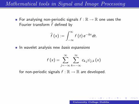
For analysing non-periodic signals f : R→ R one uses theFourier transform f̂ defined by
f̂ (x) :=
∫ ∞−∞
f (t) e−itxdt.
In wavelet analysis new basis expansions
f (x) =∞∑
j=−∞
∞∑k=−∞
ck,jψj ,k (x)
for non-periodic signals f : R→ R are developed.
Wavelets are used for data compression in JPEG 2000, DjVuand ECW for still images, REDCODE, CineForm, the BBC’sDirac, and Ogg Tarkin for video.
University College Dublin
Mathematical tools in Signal and Image Processing
For analysing non-periodic signals f : R→ R one uses theFourier transform f̂ defined by
f̂ (x) :=
∫ ∞−∞
f (t) e−itxdt.
In wavelet analysis new basis expansions
f (x) =∞∑
j=−∞
∞∑k=−∞
ck,jψj ,k (x)
for non-periodic signals f : R→ R are developed.
Wavelets are used for data compression in JPEG 2000, DjVuand ECW for still images, REDCODE, CineForm, the BBC’sDirac, and Ogg Tarkin for video.
University College Dublin

Wavelets
The Fourier transform f̂ (x) :=∫∞−∞ f (t) e−itxdt is an
important tool in physics and mathematics.
Alternative Transforms have been introduced: e.g. ”Gabortransform” (time-frequency analysis) or ”Calderon transform”.
In 1970’s J. Morlet (a geophysical engineer) introduced thewavelet transform
Wψf (x , s) = |s|−d/2∫
Rd
f (t)ψ
(t − x
s
)dt
for a function f ∈ L2(Rd).
There are many choices for a ”wavelet function” ψ ∈ L2(Rd).
The variable s is a scaling parameter (or dilation) andchanging s is like zooming in/out.
Two important ingredients: translation and dilation (scaling).
University College Dublin

Wavelets
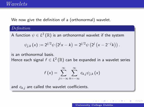
We now give the definition of a (orthonormal) wavelet.
Definition
A function ψ ∈ L2 (R) is an orthonormal wavelet if the system
ψj ,k (x) := 2j/2ψ(2jx − k
)= 2j/2ψ
(2j(x − 2−jk
)).
is an orthonormal basis.
Hence each signal f ∈ L2 (R) can be expanded in a wavelet series
f (x) =∞∑
j=−∞
∞∑k=−∞
ck,jψj ,k (x)
and ck,j are called the wavelet coefficients.
University College Dublin

Wavelets
We now give the definition of a (orthonormal) wavelet.
Definition
A function ψ ∈ L2 (R) is an orthonormal wavelet if the system
ψj ,k (x) := 2j/2ψ(2jx − k
)= 2j/2ψ
(2j(x − 2−jk
)).
is an orthonormal basis.Hence each signal f ∈ L2 (R) can be expanded in a wavelet series
f (x) =∞∑
j=−∞
∞∑k=−∞
ck,jψj ,k (x)
and ck,j are called the wavelet coefficients.
University College Dublin

The breakthrough of Ingrid Daubechies in 1988
TheoremFor each natural number m one can construct a waveletψ ∈ Cm (R) with compact support.
Wavelets can be constructed in a schematic way using thefollowing result of S. Mallat and Y. Meyer in 1988:
Theorem
Let Vj , j ∈ Z, be a Multiresolutional Analysis of L2 (R) with scalingfunction ϕ. Then there exists a wavelet ψ which is explicitlyconstructed in terms of the scaling function ϕ.
University College Dublin
Multiresolutional Analysis
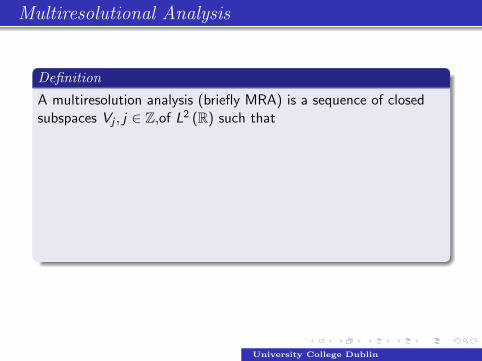
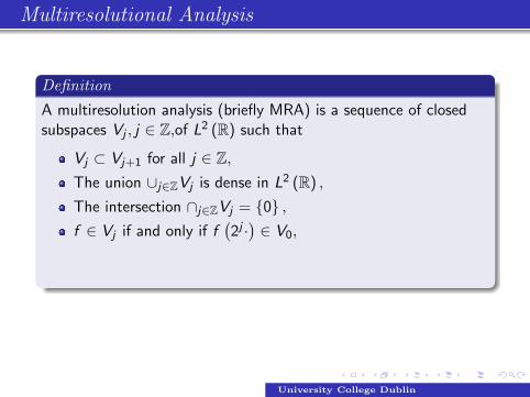
Definition
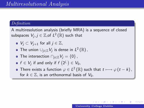
A multiresolution analysis (briefly MRA) is a sequence of closedsubspaces Vj , j ∈ Z,of L2 (R) such that
Vj ⊂ Vj+1 for all j ∈ Z,The union ∪j∈ZVj is dense in L2 (R) ,
The intersection ∩j∈ZVj = {0} ,f ∈ Vj if and only if f
(2j ·)∈ V0,
There exists a function ϕ ∈ L2 (R) such that t 7−→ ϕ (t − k) ,for k ∈ Z, is an orthonormal basis of V0.
The function ϕ in the last Definition is usually called the scalingfunction; it is also called the father wavelet.
University College Dublin

Multiresolutional Analysis
Definition
A multiresolution analysis (briefly MRA) is a sequence of closedsubspaces Vj , j ∈ Z,of L2 (R) such that
Vj ⊂ Vj+1 for all j ∈ Z,
The union ∪j∈ZVj is dense in L2 (R) ,
The intersection ∩j∈ZVj = {0} ,f ∈ Vj if and only if f
(2j ·)∈ V0,
There exists a function ϕ ∈ L2 (R) such that t 7−→ ϕ (t − k) ,for k ∈ Z, is an orthonormal basis of V0.
The function ϕ in the last Definition is usually called the scalingfunction; it is also called the father wavelet.
University College Dublin

Multiresolutional Analysis
Definition
A multiresolution analysis (briefly MRA) is a sequence of closedsubspaces Vj , j ∈ Z,of L2 (R) such that
Vj ⊂ Vj+1 for all j ∈ Z,The union ∪j∈ZVj is dense in L2 (R) ,
The intersection ∩j∈ZVj = {0} ,f ∈ Vj if and only if f
(2j ·)∈ V0,
There exists a function ϕ ∈ L2 (R) such that t 7−→ ϕ (t − k) ,for k ∈ Z, is an orthonormal basis of V0.
The function ϕ in the last Definition is usually called the scalingfunction; it is also called the father wavelet.
University College Dublin

Multiresolutional Analysis
Definition
A multiresolution analysis (briefly MRA) is a sequence of closedsubspaces Vj , j ∈ Z,of L2 (R) such that
Vj ⊂ Vj+1 for all j ∈ Z,The union ∪j∈ZVj is dense in L2 (R) ,
The intersection ∩j∈ZVj = {0} ,
f ∈ Vj if and only if f(2j ·)∈ V0,
There exists a function ϕ ∈ L2 (R) such that t 7−→ ϕ (t − k) ,for k ∈ Z, is an orthonormal basis of V0.
The function ϕ in the last Definition is usually called the scalingfunction; it is also called the father wavelet.
University College Dublin
Multiresolutional Analysis
Definition
A multiresolution analysis (briefly MRA) is a sequence of closedsubspaces Vj , j ∈ Z,of L2 (R) such that
Vj ⊂ Vj+1 for all j ∈ Z,The union ∪j∈ZVj is dense in L2 (R) ,
The intersection ∩j∈ZVj = {0} ,f ∈ Vj if and only if f
(2j ·)∈ V0,
There exists a function ϕ ∈ L2 (R) such that t 7−→ ϕ (t − k) ,for k ∈ Z, is an orthonormal basis of V0.
The function ϕ in the last Definition is usually called the scalingfunction; it is also called the father wavelet.
University College Dublin
Nonstationary MRA
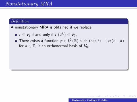
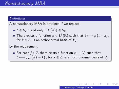
DefinitionA nonstationary MRA is obtained if we replace
f ∈ Vj if and only if f(2j ·)∈ V0,
There exists a function ϕ ∈ L2 (R) such that t 7−→ ϕ (t − k) ,for k ∈ Z, is an orthonormal basis of V0,
by the requirement
For each j ∈ Z there exists a function ϕj ∈ Vj such thatt 7−→ ϕm
(2j t − k
), for k ∈ Z, is an orthonormal basis of Vj .
Fact: Most of the results of MRA carry over in a rather obviousway to non-stationary MRA (by adding just an additional index jto the scaling function ϕ) .
University College Dublin
Nonstationary MRA
DefinitionA nonstationary MRA is obtained if we replace
f ∈ Vj if and only if f(2j ·)∈ V0,
There exists a function ϕ ∈ L2 (R) such that t 7−→ ϕ (t − k) ,for k ∈ Z, is an orthonormal basis of V0,
by the requirement
For each j ∈ Z there exists a function ϕj ∈ Vj such thatt 7−→ ϕm
(2j t − k
), for k ∈ Z, is an orthonormal basis of Vj .
Fact: Most of the results of MRA carry over in a rather obviousway to non-stationary MRA (by adding just an additional index jto the scaling function ϕ) .
University College Dublin
Subdivison Schemes
Subdivision schemes are used in 3D Computer graphics forrepresenting smooth surfaces.
In the simplest case the data are given by a functionf : Zm → R and one computes
f
(j
2k+1
)inductively for k ∈ Z (and j ∈ Zm) from finitely many
function values on level k , hence from f(
j2k
)by a simple
subdivision rule.
An important Example of Deslaurier/Dubuc: The
intermediate value f(
j2k+1
)is determined by taking the value
of a cubic polynomial at j/2k+1 interpolating four neighboringpoints at the previous level k .
University College Dublin

Subdivison Schemes
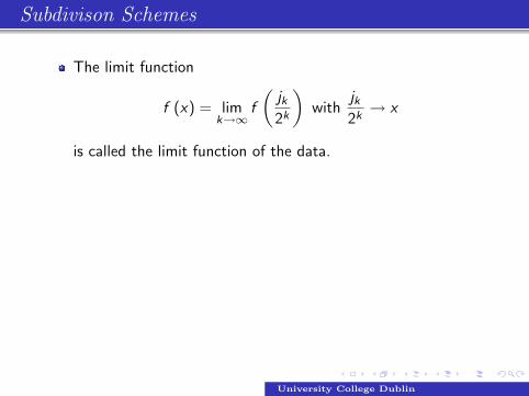
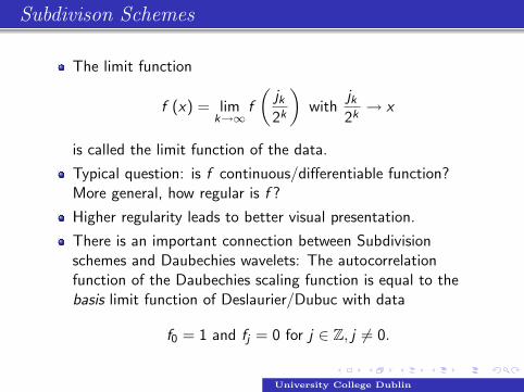
The limit function
f (x) = limk→∞
f
(jk2k
)with
jk2k→ x
is called the limit function of the data.
Typical question: is f continuous/differentiable function?More general, how regular is f ?
Higher regularity leads to better visual presentation.
There is an important connection between Subdivisionschemes and Daubechies wavelets: The autocorrelationfunction of the Daubechies scaling function is equal to thebasis limit function of Deslaurier/Dubuc with data
f0 = 1 and fj = 0 for j ∈ Z, j 6= 0.
University College Dublin
Subdivison Schemes
The limit function
f (x) = limk→∞
f
(jk2k
)with
jk2k→ x
is called the limit function of the data.
Typical question: is f continuous/differentiable function?More general, how regular is f ?
Higher regularity leads to better visual presentation.
There is an important connection between Subdivisionschemes and Daubechies wavelets: The autocorrelationfunction of the Daubechies scaling function is equal to thebasis limit function of Deslaurier/Dubuc with data
f0 = 1 and fj = 0 for j ∈ Z, j 6= 0.
University College Dublin

New methods in Subdivision
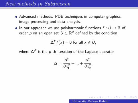
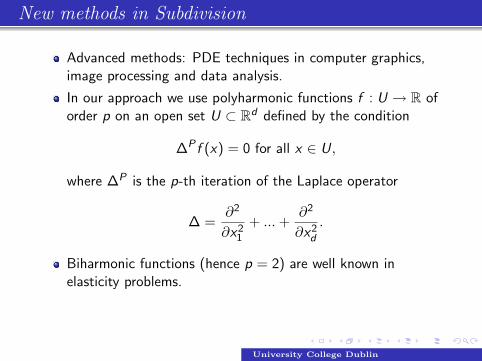
Advanced methods: PDE techniques in computer graphics,image processing and data analysis.
In our approach we use polyharmonic functions f : U → R oforder p on an open set U ⊂ Rd defined by the condition
∆P f (x) = 0 for all x ∈ U,
where ∆P is the p-th iteration of the Laplace operator
∆ =∂2
∂x21
+ ...+∂2
∂x2d
.
Biharmonic functions (hence p = 2) are well known inelasticity problems.
We consider polyharmonic functions of order p as amultivariate generalization of polynomials of degree p.
University College Dublin

New methods in Subdivision
Advanced methods: PDE techniques in computer graphics,image processing and data analysis.
In our approach we use polyharmonic functions f : U → R oforder p on an open set U ⊂ Rd defined by the condition
∆P f (x) = 0 for all x ∈ U,
where ∆P is the p-th iteration of the Laplace operator
∆ =∂2
∂x21
+ ...+∂2
∂x2d
.
Biharmonic functions (hence p = 2) are well known inelasticity problems.
We consider polyharmonic functions of order p as amultivariate generalization of polynomials of degree p.
University College Dublin
New Ansatz: Polyharmonic Subdivision
Define a subdivision scheme in R2 where the data are givenon the parallel lines
j × R for j ∈ Z.
Use interpolation with polyharmonic functions on equidistantlines j × R for defining the value for the function for the“half-integers lines”
{k + 1
2
}× R.
By iteration we obtain a ”polyharmonic subdivision scheme”.
We can reduce the ”polyharmonic subdivision scheme” via afamily of non-stationary univariate subdivision schemes.
In these univariate schemes the interpolation with”polynomials of degree 2n − 1” is modified to interpolationwith certain classes of exponential polynomials, so functionsof the form
p (x) = a0eλ0x + ...+ a2n−1eλ2n−1x .
University College Dublin

Generalized Daubechies wavelets
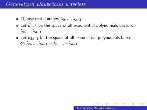
Choose real numbers λ0, ..., λn−1.
Let En−1 be the space of all exponential polynomials based onλ0, ..., λn−1.
Let E2n−1 be the space of all exponential polynomials basedon λ0, ..., λn−1,−λ0, ...,−λn−1.
We shall construct Daubechies type wavelets reconstructingthe space En−1.
Taking λ0 = ... = λn−1 = 0 one obtains the classicalDaubechies wavelets.
Consider the (non-stationary) subdivision scheme usinginterpolating exponential polynomials in E2n−1.
A non-trivial analysis of the non-stationary symbol a[k] (z) ofthe subdivision schemes shows that it is non-negative on theunit circle.
University College Dublin

Generalized Daubechies wavelets
Choose real numbers λ0, ..., λn−1.
Let En−1 be the space of all exponential polynomials based onλ0, ..., λn−1.
Let E2n−1 be the space of all exponential polynomials basedon λ0, ..., λn−1,−λ0, ...,−λn−1.
We shall construct Daubechies type wavelets reconstructingthe space En−1.
Taking λ0 = ... = λn−1 = 0 one obtains the classicalDaubechies wavelets.
Consider the (non-stationary) subdivision scheme usinginterpolating exponential polynomials in E2n−1.
A non-trivial analysis of the non-stationary symbol a[k] (z) ofthe subdivision schemes shows that it is non-negative on theunit circle.
University College Dublin
Generalized Daubechies wavelets
The Fejer-Riesz lemma provides a decomposition
a[k](e iω) =1
2|M [k](e iω)|2 and M [k] (1) > 0
for a Laurent polynomial M [k](z) with real coefficients.
The scaling functions ϕm for a non-stationary MRA aredefined by
ϕ̂m (ω) =∞∏
k=1
M [m+k−1](
ei ω
2k
)2
.
University College Dublin
Regularity of generalized Daubechies wavelets
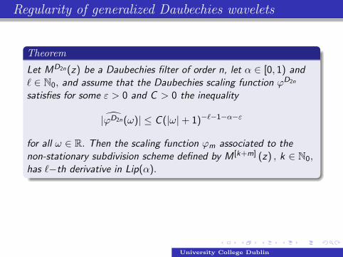
Theorem
Let MD2n(z) be a Daubechies filter of order n, let α ∈ [0, 1) and` ∈ N0, and assume that the Daubechies scaling function ϕD2n
satisfies for some ε > 0 and C > 0 the inequality
|ϕ̂D2n(ω)| ≤ C (|ω|+ 1)−`−1−α−ε
for all ω ∈ R. Then the scaling function ϕm associated to thenon-stationary subdivision scheme defined by M [k+m] (z) , k ∈ N0,has `−th derivative in Lip(α).
Conjecture: The generalized Daubechies wavelets for real valuesλ0, ..., λn−1 have the same regularity as the classical Daubechieswavelets of order n.
University College Dublin

Regularity of generalized Daubechies wavelets
Theorem
Let MD2n be the Daubechies filter of order n and let λ0, ..., λn−1
be real numbers. Then there exists a non-stationary Daubechiestype subdivision scheme {M [k](z)} which is asymptoticallyequivalent to MD2n .
N. Dyn, D. Levin, O. Kounchev, H. Render: Regularity ofgeneralized Daubechies wavelets reproducing exponentialpolynomials with realvalued parametersto appear in ACHA: Applied Computational HarmonicAnalysis.
University College Dublin
Recommended


![On the Zeros of Daubechies Orthogonal and Biorthogonal ... · wavelets were proved to reside inside the unit circle [5], and better limits for these roots based on a generalization](https://img.pdfslide.us/doc/110x75/5e8c0ab1eeeec952fe19f2dd/on-the-zeros-of-daubechies-orthogonal-and-biorthogonal-wavelets-were-proved.jpg)