Embed Size (px)
Citation preview
mathematics of computationvolume 63, number 207july 1994, pages 155-173
WAVELET CALCULUS AND FINITE DIFFERENCE OPERATORS
KENT McCORMICK AND RAYMOND O. WELLS, JR.
Abstract. This paper shows that the naturally induced discrete differentiation
operators induced from a wavelet-Galerkin finite-dimensional approximation to
a standard function space approximates differentiation with an error of order
0(h2d+2), where d is the degree of the wavelet system. The degree of a wavelet
system is defined as one less than the degree of the lowest-order nonvanishing
moment of the fundamental wavelet. We consider in this paper compactly
supported wavelets of the type introduced by Daubechies in 1988. The induced
differentiation operators are described in terms of connection coefficients which
are intrinsically defined functional invariants of the wavelet system (defined
as L2 inner products of derivatives of wavelet basis functions with the basis
functions themselves). These connection coefficients can be explicitly computed
without quadrature and they themselves have key moment-vanishing properties
proved in this paper which are dependent upon the degree of the wavelet system.
This is the basis for the proof of the principal results concerning the degree of
approximation of the differentiation operator by the wavelet-Galerkin discrete
differentiation operator.
1. Introduction
The recently discovered compactly supported wavelets of Daubechies [4] have
proven to be a useful tool in the numerical solutions of partial differential equa-
tions (see [7, 12, 17, 20, 19, 16] for recent numerical solutions of partial differ-
ential equations using wavelet-Galerkin techniques. In each of the papers abovethe notion of connection coefficients has played a key role in the approximations
of partial derivatives as well as nonlinear terms in the wavelet discretization of
the differential equations. Connection coefficients and some of their properties
and algorithms for computing them are described in [11] and [1].The purpose of this paper is to show that there is a relationship between
discrete differentiation using connection coefficients and discrete differentiation
using finite difference operators.
A certain class of finite difference operators have the property that operating
on the discretization of a polynomial of degree d is equivalent to differentiating
the polynomials and then discretizing. This implies that the finite difference
operator approximates the derivative up to order d, and conversely. Let us
Received by the editor November 5, 1992.
1991 Mathematics Subject Classification. Primary 65D25; Secondary 65L12, 42C99.Key words and phrases. Wavelets, finite difference operators, Galerkin approximation,
connection coefficients.
©1994 American Mathematical Society
0025-5718/94 $1.00+ $.25 per page
155
License or copyright restrictions may apply to redistribution; see https://www.ams.org/journal-terms-of-use
156 KENT McCORMICK AND R. O. WELLS, JR.
explain what this means. Consider a lattice
A = {x0 + ih}, ¡eZ,
in R, for some fixed h e R. Let x¡ = Xo + ih denote a generic point of A,
and let C(A) denote the continuous ( = arbitrary) real-valued functions on A.
Then a finite difference operator V is a mapping of the form
(1.1) C(A)ZC(A):f(x,)~g(x,),
where
#i kW7(1.2) g(x,) = Vf(xi)= £ -J-f(Xi + kh)
k=-N,
and the wk are the weights of the finite difference operator. For instance, there
is a classical 5-point symmetric difference operator of the form
V4(/)(x,) = -irj- [f(x, - 2ft) - Sf(x, -h) + if(Xi + h)- f(Xi + 2/0](1.3) un
= m [/(x'-2) - 8/(x'-,) + 8/^i+1) - f{Xi+2)] '
and the first form of the operator indicates the origin of the name finite differ-
ence operator. This finite difference operator has the simpler form (defined at
any point xeR)
N k
(1.4) V/(x)= £ 0Lf(x + kh),k=-N
which is independent of the point x where it is evaluated. This is the only kind
of finite difference operators we shall consider in this paper.
By using wavelet interpolation to discretize continuous functions (see [20]),
and by using the connection coefficients determined by the wavelet system to
obtain a discrete approximation, one obtains a wavelet discrete differentiation
operator of the form
2*-2
(1.5) Dj(f)(x0)= J2 2JYkf(xo + kh).k=-2g+2
Here, h = 2~J is the mesh size for some fixed scaling J of the wavelet system,
and
yk1 0 = / (p'(x)tp(x - k)dx
are connection coefficients as defined in §3 below, where <p(x) is the scaling
function of the given wavelet system.
The main point of this paper is that there is a strong relation between the
classical finite difference operators and the induced discrete wavelet differenti-
License or copyright restrictions may apply to redistribution; see https://www.ams.org/journal-terms-of-use
WAVELET CALCULUS AND FINITE DIFFERENCE OPERATORS 157
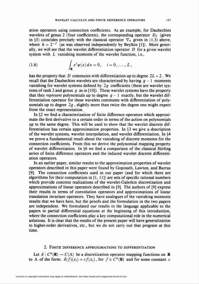
ation operators using connection coefficients. As an example, for Daubechies
wavelets of genus 2 (four coefficients), the corresponding operator Dj (given
in §5) coincides precisely with the classical operator V4 given in (1.3) above,
where h = 2~J (as was observed independently by Beylkin [1]). More gener-
ally, we will see that the wavelet differentiation operator D for a given wavelet
system with L vanishing moments of the wavelet function, i.e.,
(1.6) Í x!y/(x)dx = 0, i = 0,...,L,Jr
has the property that D commutes with differentiation up to degree 2L + 2. We
recall that the Daubechies wavelets are characterized by having g - 1 moments
vanishing for wavelet systems defined by 2g coefficients (these are wavelet sys-
tems of rank 2 and genus g as in [ 10]). These wavelet systems have the property
that they represent polynomials up to degree g - 1 exactly, but the wavelet dif-
ferentiation operator for these wavelets commutes with differentiation of poly-
nomials up to degree 2g, slightly more than twice the degree one might expect
from the exact representation.
In §2 we find a characterization of finite difference operators which approxi-
mate the first derivative to a certain order in terms of the action on polynomials
up to the same degree. This will be used to show that the wavelet discrete dif-
ferentiation has certain approximation properties. In §3 we give a description
of the wavelet systems, wavelet interpolation, and wavelet differentiation. In §4
we prove a fundamental result about the vanishing of discrete moments for the
connection coefficients. From this we derive the polynomial mapping propertyof wavelet differentiation. In §6 we find a comparison of the classical Stirling
series of finite difference operators and the induced wavelet discrete differenti-
ation operators.
In an earlier paper, similar results to the approximation properties of wavelet
operators described in this paper were found by Gopinath, Lawton, and Burras
[9]. The connection coefficients used in our paper (and for which there are
algorithms for their computation in [1, 11]) are sets of specific rational numbers
which provide concrete realizations of the wavelet-Galerkin discretization and
approximations of linear operators described in [9]. The authors of [9] expresstheir results in terms of convolution operators and approximations of lineartranslation invariant operators. They have analogues of the vanishing moments
results that we have here, but the proofs and the formulation in the two papers
are independent. We formulated our results in the language applicable to the
papers in partial differential equations at the beginning of this introduction,
where the connection coefficients play a key computational role in the numerical
solutions. It is clear that the results of the present paper will have generalization
to higher-order derivatives, etc., but we do not carry out that program at this
time.
2. Finite difference approximations to differentiation
Let ô : Ck(R) —► C(A) be a discretization operator mapping functions on R
to A of the form: S(f)(x¡) = cf(x¡), for / e C*(R) and for some constant c
License or copyright restrictions may apply to redistribution; see https://www.ams.org/journal-terms-of-use
158 KENT McCORMICK AND R. O. WELLS, JR.
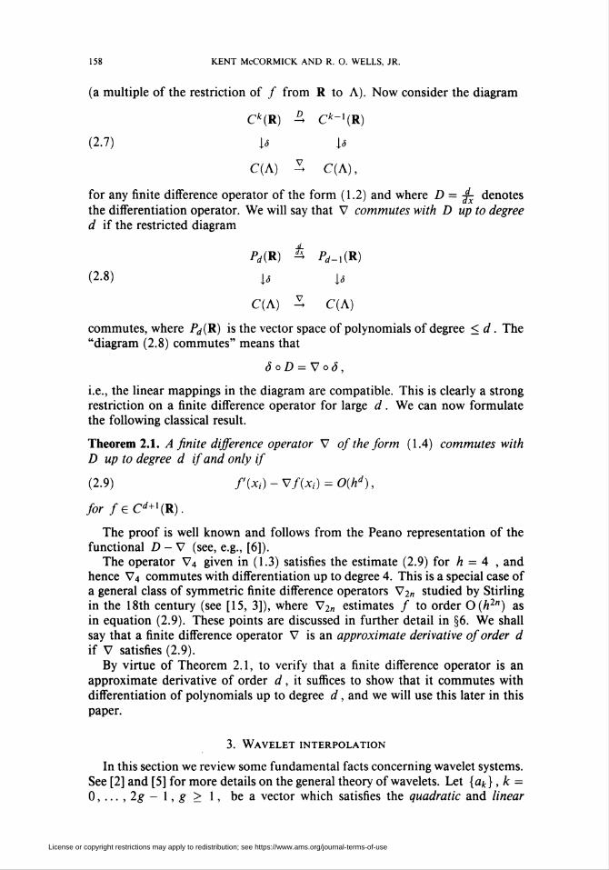
(a multiple of the restriction of / from R to A). Now consider the diagram
Ck(R) -£ Ck~x(R)
(2.1) [s is
C(A) ^ C(A),
for any finite difference operator of the form (1.2) and where D = -£¿ denotes
the differentiation operator. We will say that V commutes with D up to degreed if the restricted diagram
Pd(R) % Prf-i(R)
(2.8) n is
C(A) Z C(A)
commutes, where Pd(R) is the vector space of polynomials of degree <d. The
"diagram (2.8) commutes" means that
SoD = VoS,
i.e., the linear mappings in the diagram are compatible. This is clearly a strong
restriction on a finite difference operator for large d. We can now formulate
the following classical result.
Theorem 2.1. A finite difference operator V of the form (1.4) commutes with
D up to degree d if and only if
(2.9) f'(x,)-Vf(x,) = 0(hd),
for f€Cd+x(R).
The proof is well known and follows from the Peano representation of the
functional D - V (see, e.g., [6]).The operator V4 given in (1.3) satisfies the estimate (2.9) for ft = 4 , and
hence V4 commutes with differentiation up to degree 4. This is a special case of
a general class of symmetric finite difference operators V2„ studied by Stirling
in the 18th century (see [15, 3]), where V2n estimates / to order O (ft2") as
in equation (2.9). These points are discussed in further detail in §6. We shall
say that a finite difference operator V is an approximate derivative of order d
if V satisfies (2.9).By virtue of Theorem 2.1, to verify that a finite difference operator is an
approximate derivative of order d, it suffices to show that it commutes with
differentiation of polynomials up to degree d, and we will use this later in this
paper.
3. Wavelet interpolation
In this section we review some fundamental facts concerning wavelet systems.
See [2] and [5] for more details on the general theory of wavelets. Let {ak}, k =
0,...,2g-l,g>l, be a vector which satisfies the quadratic and linear
License or copyright restrictions may apply to redistribution; see https://www.ams.org/journal-terms-of-use
WAVELET CALCULUS AND FINITE DIFFERENCE OPERATORS 159
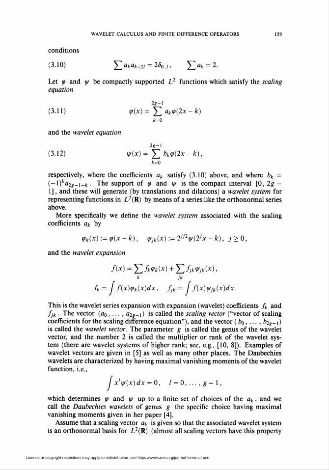
conditions
(3.10) ^akak+2t = 2öoj, Y^ak = 2.
Let <p and yi be compactly supported L2 functions which satisfy the scaling
equation
2*-1
(3.11) <p(x) = y] aktp(2x - k)k=0
and the wavelet equation
2g-i
(3.12) ¥(x)=YJh9(2x-k),k=0
respectively, where the coefficients ak satisfy (3.10) above, and where bk =
(-l)ka2g_X-k . The support of tp and y/ is the compact interval [0, 2g -
1], and these will generate (by translations and dilations) a wavelet system for
representing functions in L2(R) by means of a series like the orthonormal seriesabove.
More specifically we define the wavelet system associated with the scaling
coefficients ak by
(pk(x) := <p(x - k), y/jk(x) := 2j/2y/(2jx -k), j > 0,
and the wavelet expansion
f(x) = Y^fk<Pk(x) + ¿\lfjkVjk(x),k jk
fk = J f(x)tpk(x)dx, fjk = J f(x)y/jk(x)dx.
This is the wavelet series expansion with expansion (wavelet) coefficients fk and
fjk ■ The vector (ao, ... , a2g_x) is called the scaling vector ("vector of scalingcoefficients for the scaling difference equation"), and the vector (bo, ... , b2g-X)
is called the wavelet vector. The parameter g is called the genus of the wavelet
vector, and the number 2 is called the multiplier or rank of the wavelet sys-
tem (there are wavelet systems of higher rank; see, e.g., [10, 8]). Examples of
wavelet vectors are given in [5] as well as many other places. The Daubechies
wavelets are characterized by having maximal vanishing moments of the wavelet
function, i.e.,
Jxly/(x)dx = 0, l = 0,...,g-l,
which determines (p and y/ up to a finite set of choices of the ak, and we
call the Daubechies wavelets of genus g the specific choice having maximalvanishing moments given in her paper [4].
Assume that a scaling vector ak is given so that the associated wavelet system
is an orthonormal basis for L2(R) (almost all scaling vectors have this property
License or copyright restrictions may apply to redistribution; see https://www.ams.org/journal-terms-of-use
160 KENT McCORMICK AND R. O. WELLS, JR.
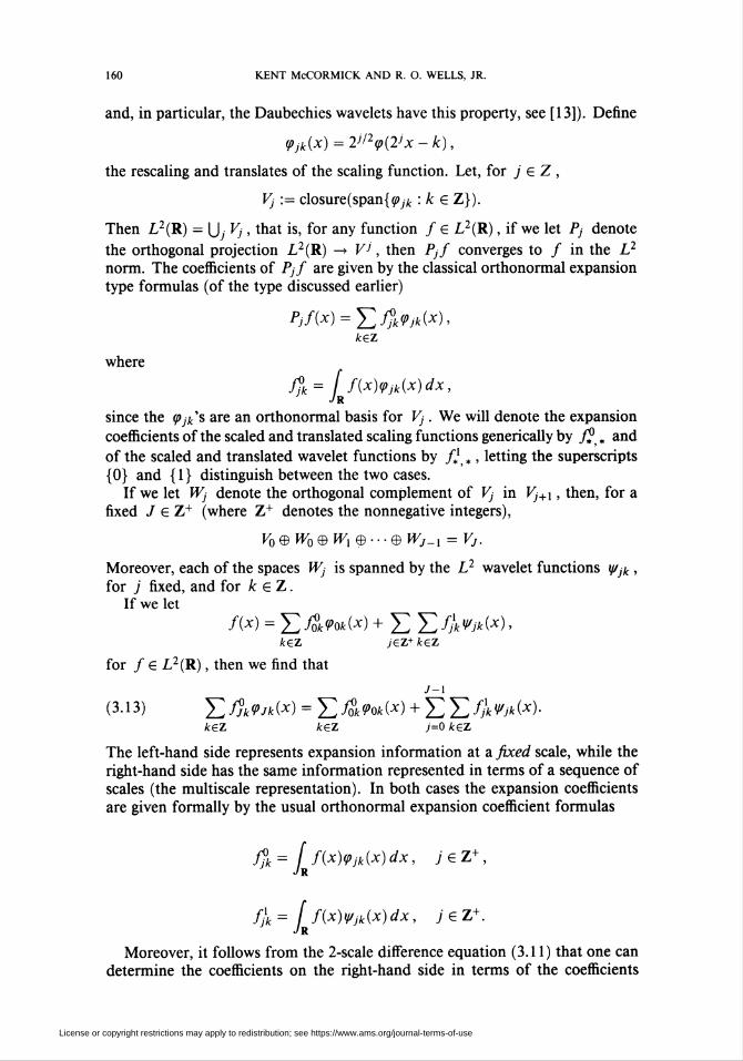
and, in particular, the Daubechies wavelets have this property, see [13]). Define
<Pjk(x) = Vl2<p(Vx-k),
the rescaling and translates of the scaling function. Let, for j e Z ,
Vj := closure(span{ç?7/t : k e Z}).
Then L2(R) = |J. Vj , that is, for any function / 6 L2(R), if we let P¡ denote
the orthogonal projection L2(R) —> VJ, then Pjf converges to / in the L2
norm. The coefficients of Pjf are given by the classical orthonormal expansion
type formulas (of the type discussed earlier)
Pjf(x) = ̂ 2ffk<pjk(x),keZ
where
fjk = j f(x)y>jk(x)dx,
since the (Pjks are an orthonormal basis for Vj. We will denote the expansion
coefficients of the scaled and translated scaling functions generically by /? « and
of the scaled and translated wavelet functions by fx », letting the superscripts
{0} and {1} distinguish between the two cases.
If we let Wj denote the orthogonal complement of Vj in Vj+X, then, for a
fixed J e Z+ (where Z+ denotes the nonnegative integers),
V0®WQ®Wi®---® Wj_x = Vj.
Moreover, each of the spaces W¡ is spanned by the L2 wavelet functions y/jk ,
for j fixed, and for k e Z.If we let
/(*) = E ./ô*po*(*) + E E fjkVjk(x),kez jez+kez
for / e L2(R), then we find that
(3.13) E^^w = EAr»w + ¿E^^(4kez kez 7=0 kez
The left-hand side represents expansion information at a fixed scale, while the
right-hand side has the same information represented in terms of a sequence of
scales (the multiscale representation). In both cases the expansion coefficients
are given formally by the usual orthonormal expansion coefficient formulas
ffk = J f(x)<pjk(x)dx, JGZ+,
fjk = J f(x)Vjk(x) dx, je Z+.
Moreover, it follows from the 2-scale difference equation (3.11) that one can
determine the coefficients on the right-hand side in terms of the coefficients
License or copyright restrictions may apply to redistribution; see https://www.ams.org/journal-terms-of-use
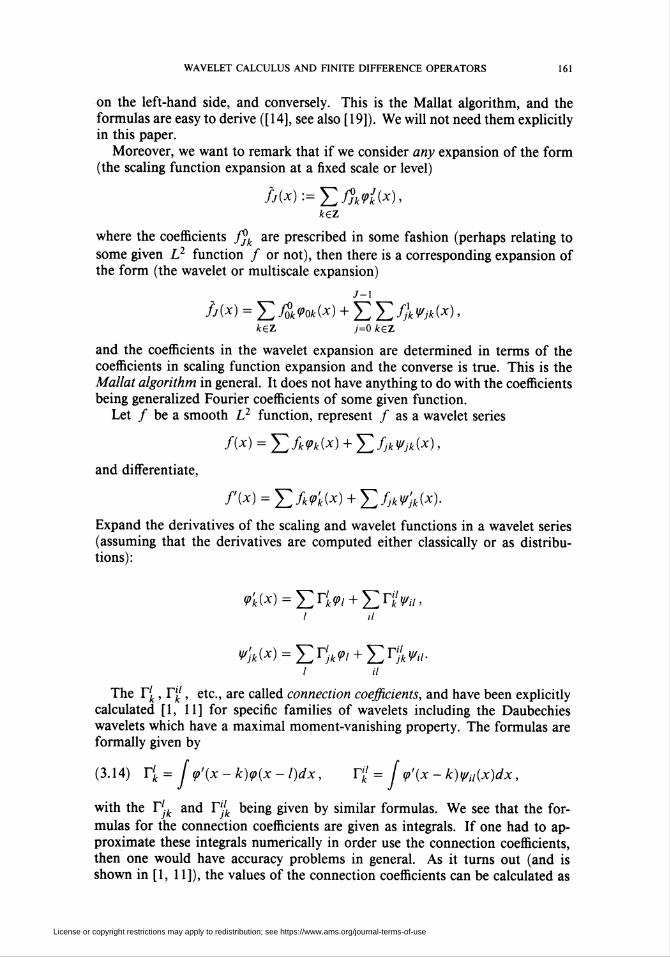
WAVELET CALCULUS AND FINITE DIFFERENCE OPERATORS 161
on the left-hand side, and conversely. This is the Mallat algorithm, and theformulas are easy to derive ([14], see also [ 19]). We will not need them explicitlyin this paper.
Moreover, we want to remark that if we consider any expansion of the form(the scaling function expansion at a fixed scale or level)
//(*):=£ fjkVk (x),kez
where the coefficients Jjk are prescribed in some fashion (perhaps relating to
some given L2 function / or not), then there is a corresponding expansion ofthe form (the wavelet or multiscale expansion)
j-i
fj(x) = E fo°k<Pok(x) + E E fjkVjk(x),kez j=o kez
and the coefficients in the wavelet expansion are determined in terms of the
coefficients in scaling function expansion and the converse is true. This is the
Mallat algorithm in general. It does not have anything to do with the coefficients
being generalized Fourier coefficients of some given function.
Let / be a smooth L2 function, represent / as a wavelet series
f(x) = Y^fk<Pk(x) + ¿\JfjkWjk(x),
and differentiate,
f(x) = Y.fMx)+Y,fjkv'jk(x)-
Expand the derivatives of the scaling and wavelet functions in a wavelet series
(assuming that the derivatives are computed either classically or as distribu-tions):
<pk(x) = J2r'k<Pi + ¿ZrkVii,l il
^W = Er;^/ + Er7^<v./ a
The Ylk, Ylkl, etc., are called connection coefficients, and have been explicitly
calculated [1, 11] for specific families of wavelets including the Daubechies
wavelets which have a maximal moment-vanishing property. The formulas areformally given by
(3.14) Y[= i(p'(x-k)(p(x-l)dx, Ykl = Í <p'(x - k)y/n(x)dx,
with the Y'jk and PL being given by similar formulas. We see that the for-
mulas for the connection coefficients are given as integrals. If one had to ap-
proximate these integrals numerically in order use the connection coefficients,then one would have accuracy problems in general. As it turns out (and is
shown in [1, 11]), the values of the connection coefficients can be calculated as
License or copyright restrictions may apply to redistribution; see https://www.ams.org/journal-terms-of-use
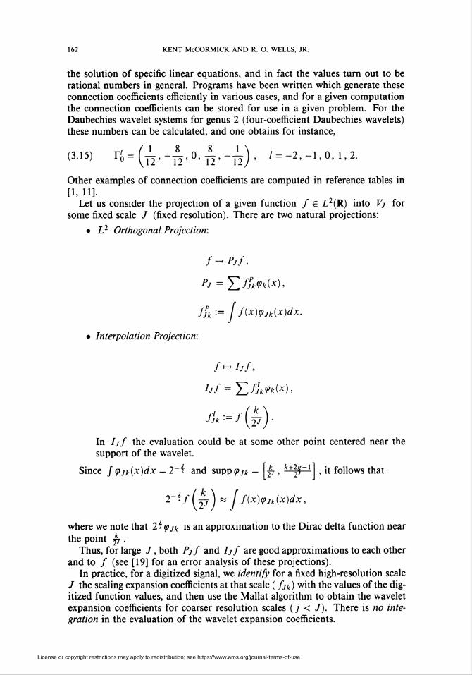
162 KENT McCORMICK AND R. O. WELLS, JR.
the solution of specific linear equations, and in fact the values turn out to berational numbers in general. Programs have been written which generate these
connection coefficients efficiently in various cases, and for a given computation
the connection coefficients can be stored for use in a given problem. For the
Daubechies wavelet systems for genus 2 (four-coefficient Daubechies wavelets)
these numbers can be calculated, and one obtains for instance,
(3.15) n=(n>4'°4'-îl)' ' = -2,-1,0,1,2.Other examples of connection coefficients are computed in reference tables in
[1,11].Let us consider the projection of a given function / e L2(R) into Vj for
some fixed scale / (fixed resolution). There are two natural projections:
• L2 Orthogonal Projection:
f^Pjf,
Pj = Y.fjk<Pk(x),
fjk '■= J f(x)(pjk(x)dx.
• Interpolation Projection:
f^hf,
hf = ^f'jk<Pk(x),
kfk--=f{V).
In Ijf the evaluation could be at some other point centered near the
support of the wavelet.
Since / (pJk(x)dx = 2~i and supp^ = -p , k+\j~x , it follows that
2~^f\2J) K I f(x)<Pjk(x)dx,
where we note that 2 i tpJk is an approximation to the Dirac delta function near
the point Jfr.Thus, for large J , both Pjf and Ijf are good approximations to each other
and to / (see [19] for an error analysis of these projections).
In practice, for a digitized signal, we identify for a fixed high-resolution scale
J the scaling expansion coefficients at that scale ( fJk) with the values of the dig-
itized function values, and then use the Mallat algorithm to obtain the wavelet
expansion coefficients for coarser resolution scales ( j < J). There is no inte-
gration in the evaluation of the wavelet expansion coefficients.
License or copyright restrictions may apply to redistribution; see https://www.ams.org/journal-terms-of-use
WAVELET CALCULUS AND FINITE DIFFERENCE OPERATORS 163
If we consider a discrete function (or digitized continuous function), which
we consider as an approximation of a given function, then we can use theconnection coefficients to calculate derivatives. We will describe this explicitly
in §5 below, but first we want to derive some important properties of connectioncoefficients as defined above.
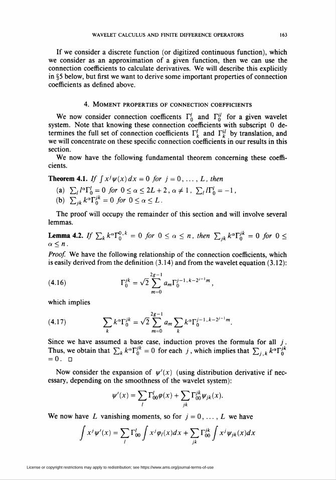
4. Moment properties of connection coefficients
We now consider connection coefficents T0 and Y'0! for a given wavelet
system. Note that knowing these connection coefficients with subscript 0 de-
termines the full set of connection coefficients Y[ and Y'kl by translation, and
we will concentrate on these specific connection coefficients in our results in thissection.
We now have the following fundamental theorem concerning these coeffi-cients.
Theorem 4.1. If jxjy/(x)dx = 0 for j = 0, ... , L, then
(a) £//Qr0 = 0/o/-0<a<2L + 2,a^l, £,/ro = -l,
(b) Y.jkkaY* = Qfor 0<a<L.
The proof will occupy the remainder of this section and will involve several
lemmas.
Lemma 4.2. // Y.k fcaro'fc = 0 for 0 < a < n, then £jk kaYjk = 0 for 0 <a < n.
Proof. We have the following relationship of the connection coefficients, which
is easily derived from the definition (3.14) and from the wavelet equation (3.12):
(4.16) Y^ = y/2^amY0-x'k-2J-'m,
m=0
which implies
(4.17) j2karo=^2ll^Y/kan~l'k~2J~>m-k m=0 k
Since we have assumed a base case, induction proves the formula for all j.
Thus, we obtain that £* kaYjk = 0 for each j, which implies that £V k ̂ ar<f= 0. D
Now consider the expansion of y'(x) (using distribution derivative if nec-
essary, depending on the smoothness of the wavelet system):
^(x) = EUoP(*) + Err>J*(*)-/ jk
We now have L vanishing moments, so for j = 0, ... , L we have
/ xJy/'(x) = J2 róo / xJtpi(x)dx + E roo / xjy/jk(x)dxI jk
License or copyright restrictions may apply to redistribution; see https://www.ams.org/journal-terms-of-use
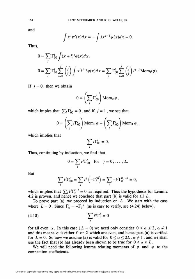
164 KENT McCORMICK AND R. O. WELLS, JR.
and
Thus,
/ xJy/'(x)dx = - jxj ' y/(x)dx = 0.
0 = Y,r'oof(x + l)j<P(x)dx,i J
0 = EróoE (j) ¡x'p-lf(x)dx = EróoE (ji) l'-'Mimif).1 i=0 V ' J I ¡=o v '
If j = 0, then we obtain
0 = ( E róo ) Momo <P,
which imples that J2i ̂ óo ~ 0, and if j = 1, we see that
0 = I E /róo J Momo 9 + ( E róo ) Momi <P >
which implies that
E/roo = 0-/
Thus, continuing by induction, we find that
o = E/>róo for ; = o,... ,l.I
But
i i i
which implies that J2ilj^o'1 = 0 as required. Thus the hypothesis for Lemma
4.2 is proven, and hence we conclude that part (b) is valid for all L.
To prove part (a), we proceed by induction on L. We start with the case
where L = 0. Since Y!0 = -Yq1 (as is easy to verify, see (4.24) below),
(4.18) E/Qró = °/
for all even a. In this case ( L = 0) we need only consider 0<a<2,a^l
and this means a is either 0 or 2 which are even, and hence part (a) is verified
for L = 0. So now we assume (a) is valid for 0 < a < 2L, a ^ 1, and we shall
use the fact that (b) has already been shown to be true for 0 < a < L.
We will need the following lemma relating moments of y> and y/ to the
connection coefficients.
License or copyright restrictions may apply to redistribution; see https://www.ams.org/journal-terms-of-use
WAVELET CALCULUS AND FINITE DIFFERENCE OPERATORS 165
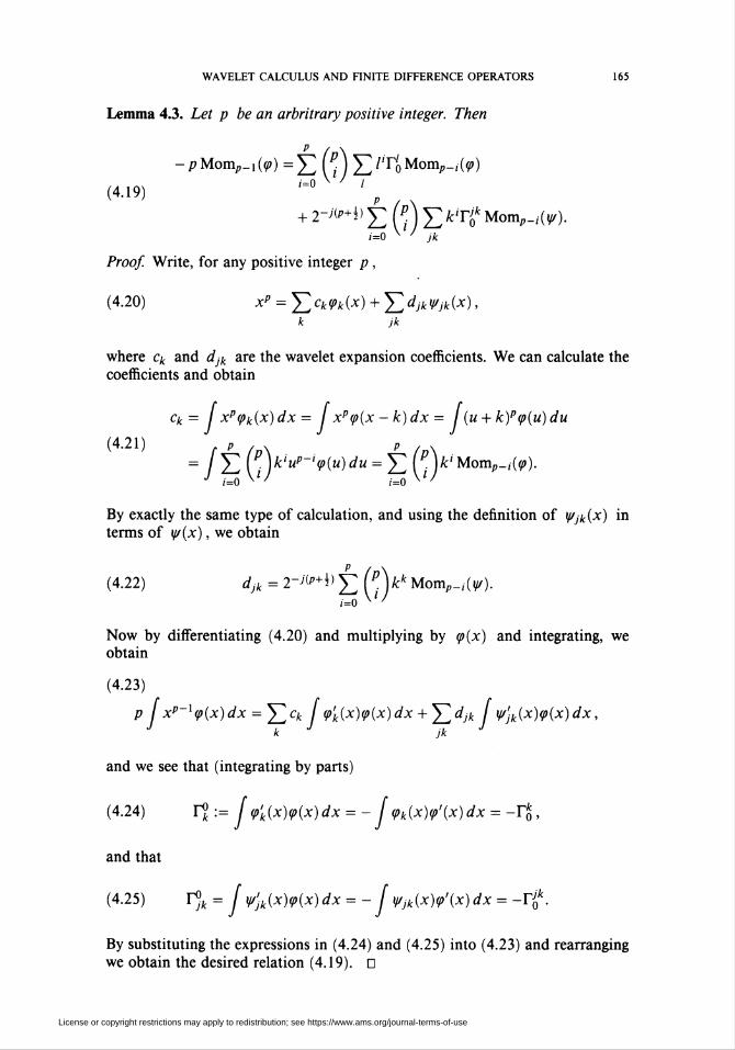
Lemma 4.3. Let p be an arbritrary positive integer. Then
(4.19)
-/»Mom,.,!» =¿ (p\ £/T0Momp_,»
1=0 ^ ' i
+ 2-A^i) ¿ Q £ fcT¿* Momp_,(^).1=0 x ' yfc
Proo/ Write, for any positive integer p,
(4.20) *P = E ck9k(x) + E djkVjk(x),k jk
where cfc and djk are the wavelet expansion coefficients. We can calculate thecoefficients and obtain
Ck = xp<pk(x)dx = xp<p(x - k)dx = j (u + k)ptp(u) du
(4.21) r p /n\ p /n\= / E d)kiup-t?(u)du = Y/ [: )kiUomp-i{9).
J 1=0 ^ ' 1=0 ^ '
By exactly the same type of calculation, and using the definition of yijk(x) in
terms of y/(x), we obtain
(4.22) djk = 2-;C+*> £ (*)** Momp_,(^).i=0
Now by differentiating (4.20) and multiplying by tp(x) and integrating, weobtain
(4.23)
p / xp~x(p(x)dx = YJCk j (p'k(x)f(x)dx + ^djk j y/'jk(x)<p(x)dx,J k J jk J
and we see that (integrating by parts)
(4.24) r° := j <p'k(x)<p(x) dx = - j <pk(x)<p'(x) dx = -Yk0 ,
and that
(4.25) Y°jk = j ys'jk(x)<p(x) dx = - J y/jk(x)<p'(x) dx = -P0k.
By substituting the expressions in (4.24) and (4.25) into (4.23) and rearranging
we obtain the desired relation (4.19). n
License or copyright restrictions may apply to redistribution; see https://www.ams.org/journal-terms-of-use
166 KENT McCORMICK. AND R. O. WELLS, JR.
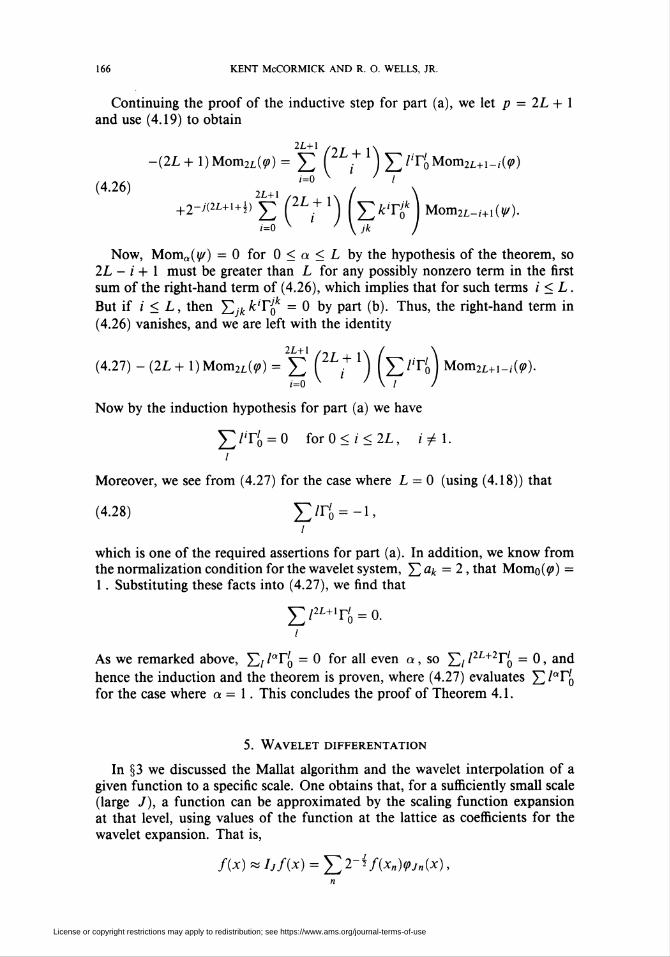
Continuing the proof of the inductive step for part (a), we let p = 2L + 1
and use (4.19) to obtain
2L+1 ,- s
-(2L+l)Mom2L(?) = £ (¿L+1)^/T/0Mom2¿+1_;^)
(4-26) 2L+1 '=° / ' X
+2-WD £ \Ltl) I Efc'rofe) Mom2L_i+1(^.
Now, Moma(^) = 0 for 0 < a < L by the hypothesis of the theorem, so
2L- i+1 must be greater than L for any possibly nonzero term in the first
sum of the right-hand term of (4.26), which implies that for such terms i < L.
But if i < L, then ^2jkk'YJ0 = 0 by part (b). Thus, the right-hand term in
(4.26) vanishes, and we are left with the identity
(4.27) - (2L+ l)Mom2L» = ¿ (2L + ^ fe^o) Mom2L+1_,».
Now by the induction hypothesis for part (a) we have
£>r0 = 0 forO</<2L, ijél.
Moreover, we see from (4.27) for the case where L = 0 (using (4.18)) that
(4.28) E/ró = -!>/
which is one of the required assertions for part (a). In addition, we know from
the normalization condition for the wavelet system, YLak = 2, that Momo» =
1 . Substituting these facts into (4.27), we find that
E/2L+lró = o.
As we remarked above, Yli la^o ~ ^ for all even a, so J2i l2L+2YlQ = 0, and
hence the induction and the theorem is proven, where (4.27) evaluates £ ^ó
for the case where a = 1. This concludes the proof of Theorem 4.1.
5. Wavelet differentation
In §3 we discussed the Mallat algorithm and the wavelet interpolation of a
given function to a specific scale. One obtains that, for a sufficiently small scale(large J), a function can be approximated by the scaling function expansion
at that level, using values of the function at the lattice as coefficients for the
wavelet expansion. That is,
f{x) « hf(x) = Y^2~^f(xn)(pJn(x),
License or copyright restrictions may apply to redistribution; see https://www.ams.org/journal-terms-of-use
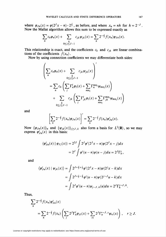
WAVELET CALCULUS AND FINITE DIFFERENCE OPERATORS 167
where g>j„(x) = <p(2Jx - n) • 2$ , as before, and where x„ = nh for ft = 2 J .
Now the Mallat algorithm allows this sum to be expressed exactly as
J2c„tpn(x)+ Y, cjk¥jk(x) = Y2~ííf^X")(PJn(x).« k "
0<j<J-l
This relationship is exact, and the coefficients ck and Cjk are linear combina-tions of the coefficients f(x„).
Now by using connection coefficients we may differentiate both sides:
/ VYCn<Pn(x)+ Y CJk{l/jk(x)
\k
0<j<J-l )
= Ec« (Er>'W+Err2vw*))n \ l mn2 )
+ E 'j*fe *%*/(*)+Eiy*w*)jk \ l "¡"2 '
0<j<J-l
and
Y,1-{f(Xn)<Pjn(x) =Y2~Íf(Xn)<p'jn(x)
Now {y>jn(x)}„ and {Wjk(x)}j>j ,k also form a DaSlS f°r L2(R), so we mayexpress <p'Jn(x) in this basis:
(<p'jn(x) | <Pjj(x)) = 22J j 2J(p'(2Jx - n)<p(2Jx - j)dx
= 2J J <p'(u - n)tp(u - j)du = 2JY{ ,
and
(<P'jn(x) I Wjk(x)) = ¡2J+^(p'(2Jx-n)y/(Vx-k)dx
= Í2J+i-¿2<p'(u-n)y/(2J-Ju-k)dx
= J 2J<p'(u - n)y/}_j,k(u)du = 2JT{~J>k.
Thus,
Y,2-lf(xn)<p'Jr,(x)n
= Y2-if(Xn)[Y2Jr'n<PJl(x) + Y2Jrn~J'SV'rs(x)) , T > J.n \ I rs J
License or copyright restrictions may apply to redistribution; see https://www.ams.org/journal-terms-of-use
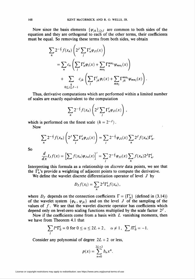
168 KENT McCORMICK AND R. O. WELLS, JR.
Now since the basis elements {Vjk}j>j are common to both sides of the
equation and they are orthogonal to each of the other terms, their coefficients
must be equal. So removing these terms from both sides, we obtain
£2-i/(*oÎ2/X;rj>//(*))
= Ec« (Er>/W+Enr2vw*))
+ E ^feiV/W + Erpiw*)).k V / m"2 I
0<j<J-l
Thus, derivative computations which are performed within a limited number
of scales are exactly equivalent to the computation
Y2-'f(Xn)\2JYT'n<Pj,(x)\ ,
which is performed on the finest scale (h = 2 J).
Now
E2-*/(x«) (2JYr„<Pj,(x)) =^2-i^w^2%)r:.n \ I J I n
So
Ijf(x) = [Yf(Xn)<PJn(x)]' = YJl-L><Pjl(x)Y,f(Xn)2JYln.d_
dx'i
Interpreting this formula as a relationship on discrete data points, we see thatthe r(,'s provide a weighting of adjacent points to compute the derivative.
We define the wavelet discrete differentiation operator of level / by
Djf(Xl) = Y2JKf(Xn),n
where Dj depends on the connection coefficients Y = {Y'n} (defined in (3.14))
of the wavelet system {tpk, y/¡k) and on the level J of the sampling of the
values of /. We see that the wavelet discrete operator has coefficients which
depend only on level-zero scaling functions multiplied by the scale factor 2J .
Now if the coefficients come from a basis with L vanishing moments, then
we have from Theorem 4.1 that
J]/Qr0 = 0for0<a<2L + 2, a ± 1, £/T0 = -1./
Consider any polynomial of degree 2L + 2 or less,
2Z.+2
p(x) = E b"x"-n=0
License or copyright restrictions may apply to redistribution; see https://www.ams.org/journal-terms-of-use
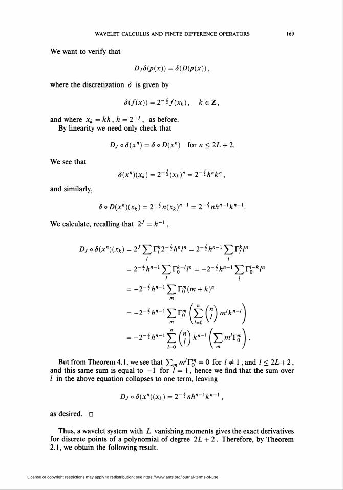
WAVELET CALCULUS AND FINITE DIFFERENCE OPERATORS 169
We want to verify that
Djô(p(x)) = ô(D(p(x)),
where the discretization 6 is given by
S(f(x)) = 2-if(xk), keZ,
and where Xk = kh,h = 2~J , as before.By linearity we need only check that
Djoô(xn) = ôoD(x") forn<2L + 2.
We see that
6(xn)(xk) = 2-i(xk)n = 2-$h"kn ,
and similarly,
ôoD(x")(Xk) = 2-in(xk)"-x =2-ink"-xkn-x.
We calculate, recalling that 2J = ft-1,
Dj oô(xn)(xk) = 2JYri2~ih"1" = 2-h"-x Yril"i i
= 2-ihn-xYro~'1" = -2-ih"-xYK~~hl"i i
= -2-ih"-xYro(m + k)"m
= -2-ih"-xY^(±(t¡)mlk"-')
m \/=0 V J )
= -2-ih"-x±(f¡)k"-'ÍY/m'YA.1=0 ^ ' \ m )
But from Theorem 4.1, we see that Y,m m'ro = 0 for / ^ 1, and / < 2L + 2,
and this same sum is equal to -1 for / = 1, hence we find that the sum over
/ in the above equation collapses to one term, leaving
Dj o S(x")(xk) = 2~inhn-xk"-x,
as desired. D
Thus, a wavelet system with L vanishing moments gives the exact derivativesfor discrete points of a polynomial of degree 2L + 2. Therefore, by Theorem
2.1, we obtain the following result.
License or copyright restrictions may apply to redistribution; see https://www.ams.org/journal-terms-of-use
170 KENT McCORMICK AND R. O. WELLS, JR.
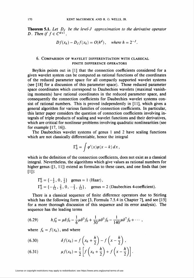
Theorem 5.1. Let Dj be the level-J approximation to the derivative operator
D. Then if f e Cd+X,
Df(xk) - Djf(xk) = 0(hd), where ft = 2~J.
6. Comparison of wavelet differentiation with classicalfinite difference operators
Beylkin points out in [1] that the connection coefficients considered for a
given wavelet system can be computed as rational functions of the coordinates
of the reduced parameter space for all compactly supported wavelet systems
(see [18] for a discussion of this parameter space). Those reduced parameterspace coordinates which correspond to Daubechies wavelets (maximal vanish-
ing moments) have rational coordinates in the reduced parameter space, and
consequently the connection coefficients for Daubechies wavelet systems con-
sist of rational numbers. This is proved independently in [11], which gives a
general algorithm for various families of connection coefficients. In particular,this latter paper considers the question of connection coefficients involving in-
tegrals of triple products of scaling and wavelet functions and their derivatives,
which are critical for nonlinear problems involving quadratic nonlinearities (see
for example [17, 16]).The Daubechies wavelet systems of genus 1 and 2 have scaling functions
which are not classically differentiable, hence the integral
t = / <p'(x)(p(x-k)dx,
which is the definition of the connection coefficients, does not exist as a classical
integral. Nevertheless, the algorithms which give values as rational numbers for
higher genus ([1, 11]) extend as formulas to these cases, and one finds that (see
[1]):
^ = {4,0,2-} genus =1 (Haar),
^o - {_T2 ' f , 0> ~\ > ~h~}, genus = 2 (Daubechies 4-coefficient).
There is a classical sequence of finite difference operators due to Stirling
which has the following form (see [3, Formula 7.5.4 in Chapter 7], and see [15]
for a more thorough discussion of this sequence and its error analysis). The
sequence has the leading terms
(6.29) hf'o = pôfo - \pô'fo + ^pô5fo - t^7o + • • • .
where fk = f(xk), and where
(6.30) ôf(xk) = f(xk + ^)-f(x-^),
(6.31) Pf(xk) = \ /(** + ï)+/(*"Î)
License or copyright restrictions may apply to redistribution; see https://www.ams.org/journal-terms-of-use
WAVELET CALCULUS AND FINITE DIFFERENCE OPERATORS 171
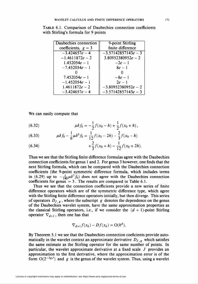
Table 6.1. Comparison of Daubechies connection coefficients
with Stirling's formula for 9 points
Daubechies connection
coefficients, g = 39-point Stirlingfinite difference
-3.424657e - 4-1.4611872e-2
1.452054e- 1-7.452054e - 1
07.452054e - 1
-1.452054e- 11.4611872e-2-3.424657e - 4
-3.57142857143e-33.80952380952e - 2
-2e- 18e- 1
0-8e-12e- 1
-3.80952380952e-2-3.57142857143e-3
We can easily compute that
(6.32)
(6.33)
(6.34)
pàfo = -j-A^o - h>> + 2^X° + ̂ '
11 2pôfo - ^pô3fo = j^f(xo - 2ft) - -f(x0 - ft)
2 1+ 3/(^0 + h) -j^f(x0 + 2ft).
Thus we see that the Stirling finite difference formulas agree with the Daubechies
connection coefficients for genus 1 and 2. For genus 3 however, one finds that the
next Stirling formula, which can be compared with the Daubechies connection
coefficients (the 9-point symmetric difference formula, which includes terms
in (6.29) up to -jfapa1 fo) does not agree with the Daubechies connectioncoefficients for genus = 3 . The results are compared in Table 6.1.
Thus we see that the connection coefficients provide a new series of finite
difference operators which are of the symmetric difference type, which agree
with the Stirling finite difference operators initially, but then diverge. This series
of operators Dj tg , where the subscript g denotes the dependence on the genus
of the Daubechies wavelet system, have the same approximation properties as
the classical Stirling operators, i.e., if we consider the (d + l)-point Stirling
operator V¿+1, then one has that
Vd+xf(Xk)-Df(xk) = 0(hd).
By Theorem 5.1 we see that the Daubechies connection coeficients provide auto-
matically in the wavelet context an approximate derivative Djg which satisfies
the same estimate as the Stirling operator for the same number of points. In
particular, the wavelet approximate derivative at a fixed scale / provides an
approximation to the first derivative, where the approximation error is of the
form 0(2-2*y) and g is the genus of the wavelet system. Thus, using a wavelet
License or copyright restrictions may apply to redistribution; see https://www.ams.org/journal-terms-of-use
172 KENT McCORMICK AND R. O. WELLS, JR.
system to represent functions includes automatically a discrete differentiation
with a predetermined rate of accuracy depending on the choice of the system,
where the error above is for the special case of Daubechies wavelet systems.
Acknowledgment
The authors would like to thank Ramesh Gopinath and Xiaodong Zhou for
useful conversations during the preparation of this paper.
Bibliography
1. G. Beylkin, On the representation of operators in bases of compactly supported wavelets, SIAM
J. Numer. Anal. 29 (1992), 1716-1740.
2. Charles Chui, Wavelet theory, Academic Press, Cambridge, MA, 1991.
3. Germund Dahlquist and Ake Björck, Numerical methods, Prentice-Hall, Englewood Cliffs,
NJ, 1974.
4. I. Daubechies, Orthonormal bases of compactly supported wavelets, Comm. Pure Appl. Math.
41 (1988), 906-966.
5. _, Ten lectures on wavelets, SIAM, Philadelphia, PA, 1992.
6. Philip J. Davis, Interpolation and approximation, Blaisdell, New York, 1963.
7. R. Glowinski, W. Lawton, M. Ravachol, and E. Tenenbaum, Wavelet solution of linear
and nonlinear elliptic, parabolic and hyperbolic problems in one dimension, Proc. Ninth
Internat. Conf. on Computing Methods in Applied Sciences and Engineering (R. Glowinski
and A. Lichnewski, eds.), SIAM, Philadelphia, PA, 1990, pp. 55-120.
8. R. Gopinath and C. S. Burrus, On the moments of the scaling function <j>, Proceedings of
ISCAS '92, May 1992, pp. 963-966.
9. R. A. Gopinath, W. M. Lawton, and C. S. Burrus, Wavelet-Galerkin approximation of linear
translation invariant operators, Proc. ICASSP-91, IEEE, 1991, pp. 2021-2024.
10. P. Heller, H. L. Resnikoff, and R. O. Wells, Jr., Wavelet matrices and the representation of
discrete functions, Wavelets: A Tutorial (Charles Chui, ed.), Academic Press, Cambridge,
MA, 1992, pp. 15-50.
11. A. Latto, H. L. Resnikoff, and E. Tenenbaum, The evaluation of connection coefficients
of compactly supported wavelets, Proc. of the French-USA Workshop on Wavelets and
Turbulence, June 1991 (Y. Maday, ed.), New York, 1994, Princeton University, Springer-
Verlag (to appear).
12. W. Lawton, W. Morrell, E. Tenenbaum, and J. Weiss, The wavelet-Galerkin method for
partial differential equations, Technical Report AD901220, Aware, Inc., 1990.
13. Wayne M. Lawton, Necessary and sufficient conditions for constructing orthonormal wavelet
bases, J. Math. Phys. 32 (1991), 57-61.
14. S. Mallat, Multiresolution approximation and wavelet orthonormal bases of /2(r), Trans.
Amer. Math. Soc. 315 (1989), 69-87.
15. L. M. Milne-Thompson, The calculus of finite differences, Macmillan, London, 1933.
16. Sam Qian and John Weiss, Wavelets and the numerical solution of partial differential
equations, J. Comput. Phys. 106 (1993), 155-175.
17. J. Weiss, Wavelets and the study of two dimensional turbulence, Proc. of the French-USA
Workshop on Wavelets and Turbulence, June 1991 (Y. Maday, ed.), New York, 1994,
Princeton University, Springer-Verlag (to appear).
License or copyright restrictions may apply to redistribution; see https://www.ams.org/journal-terms-of-use
WAVELET CALCULUS AND FINITE DIFFERENCE OPERATORS 173
18. R. O. Wells, Jr., Parametrizing smooth compactly supported wavelets, Trans. Amer. Math.
Soc. 338(1993), 919-931.
19. R. O. Wells, Jr. and Xiaodong Zhou, Wavelet interpolation and approximate solutions of
elliptic partial differential equations, Noncompact Lie Groups, Proc. of the NATO Advanced
Research Workshop (R. Wilson and E. Tanner, eds.), Kluwer, 1994 (to appear).
20. _, Wavelet solutions for the Dirichlet problem, Technical Report 92-02, Computational
Mathematics Laboratory, Rice University, 1992.
1021 Solano Avenue #6, Albany, California 94706
Department of Mathematics, Rice University, Houston, Texas 77251
License or copyright restrictions may apply to redistribution; see https://www.ams.org/journal-terms-of-use