Game Playing: Adversarial Search
2
Minimax - Nim
Assuming MIN plays first, complete the MIN/MAX tree
Assume that a utility function of
0 = a win for MIN
1 = a win for MAX
Minimax Rule
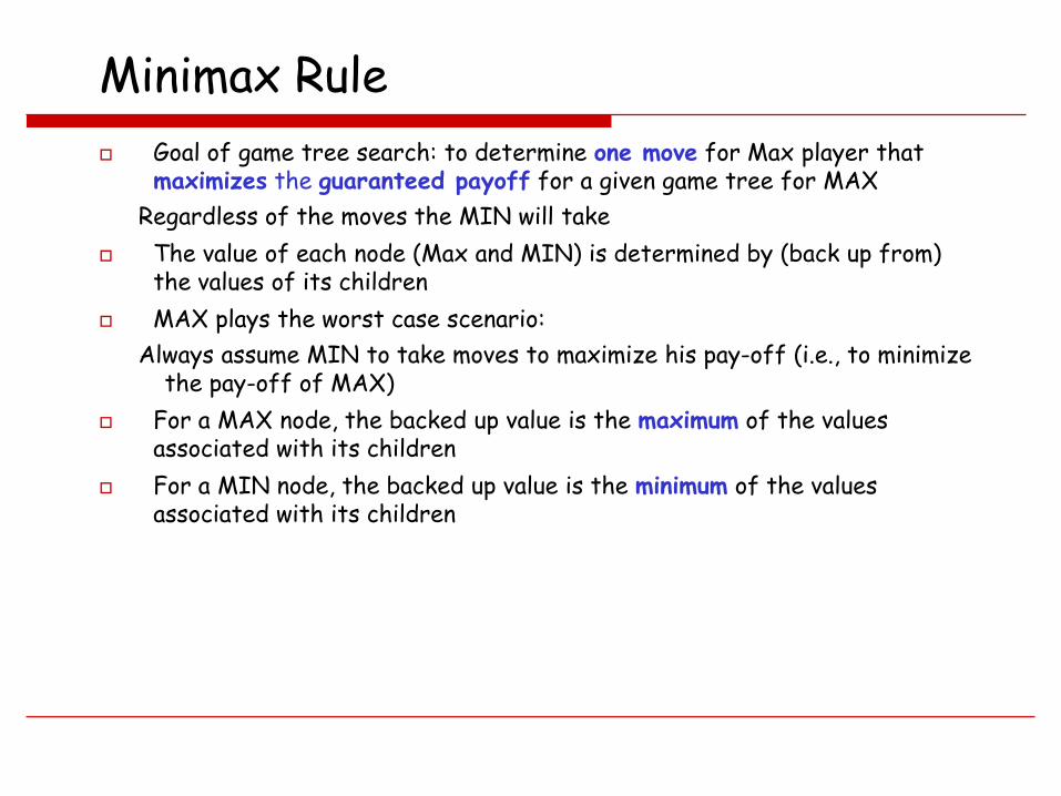
Goal of game tree search: to determine one move for Max player that maximizes the guaranteed payoff for a given game tree for MAX
Regardless of the moves the MIN will take
The value of each node (Max and MIN) is determined by (back up from) the values of its children
MAX plays the worst case scenario:
Always assume MIN to take moves to maximize his pay-off (i.e., to minimize the pay-off of MAX)
For a MAX node, the backed up value is the maximum of the values associated with its children
For a MIN node, the backed up value is the minimum of the values associated with its children
4
Minimax to a Fixed Ply-Depth
• Usually not possible to expand a game to end-game
status
– have to choose a ply-depth that is achievable with
reasonable time and resources
– absolute ‘win-lose’ values become heuristic
scores
– heuristics are devised according to knowledge of
the game
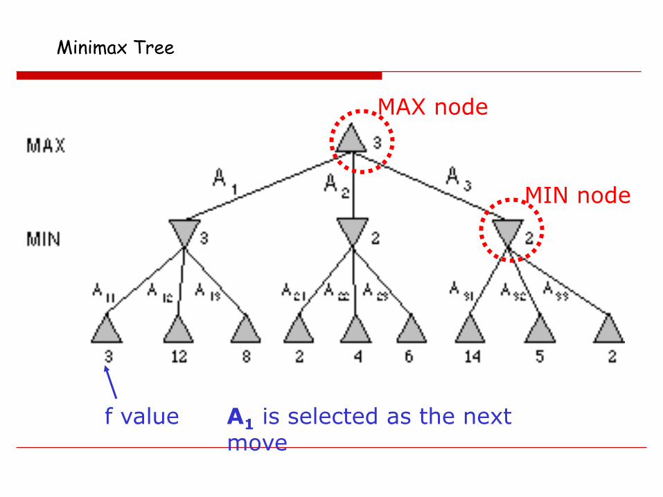
Minimax Tree
MAX node
MIN node
f value A1 is selected as the next move
Minimax procedure
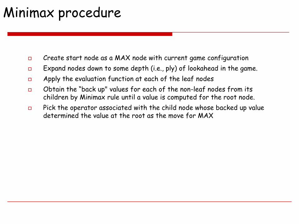
Create start node as a MAX node with current game configuration
Expand nodes down to some depth (i.e., ply) of lookahead in the game.
Apply the evaluation function at each of the leaf nodes
Obtain the “back up" values for each of the non-leaf nodes from its children by Minimax rule until a value is computed for the root node.
Pick the operator associated with the child node whose backed up value determined the value at the root as the move for MAX
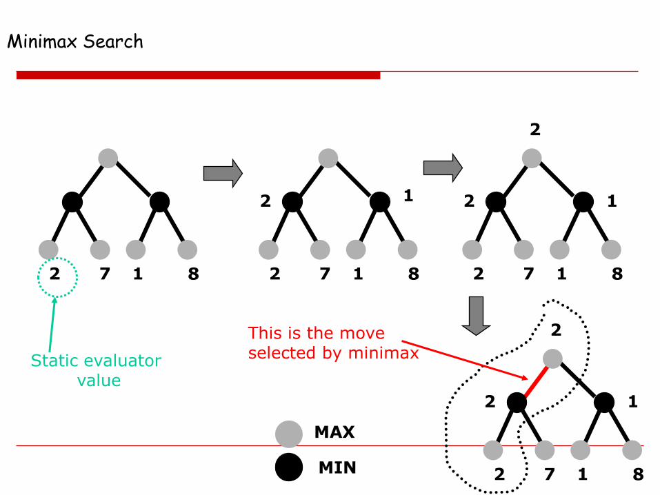
Minimax Search
2 7 1 8
MAX
MIN
2 7 1 8
2 1
2 7 1 8
2 1
2
2 7 1 8
2 1
2This is the moveselected by minimaxStatic evaluator
value
8
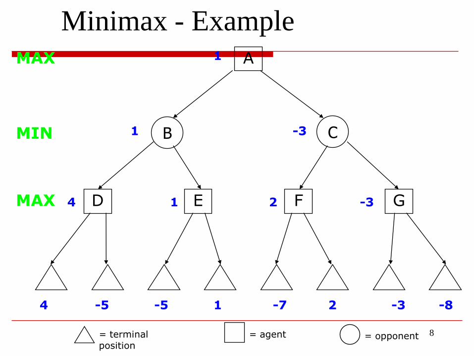
D E F G
= terminal position
= agent = opponent
4 -5 -5 1 -7 2 -3 -8
1
MAX
MIN
4 1 2 -3
MAX
1 -3B C
A
Minimax - Example
9
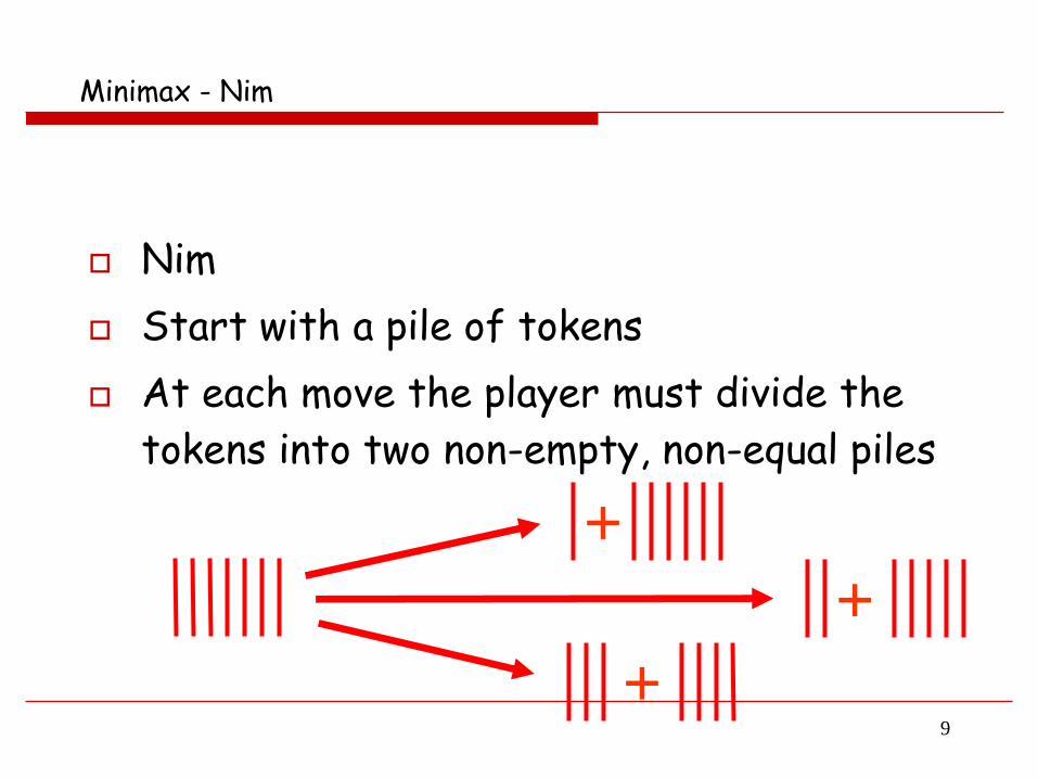
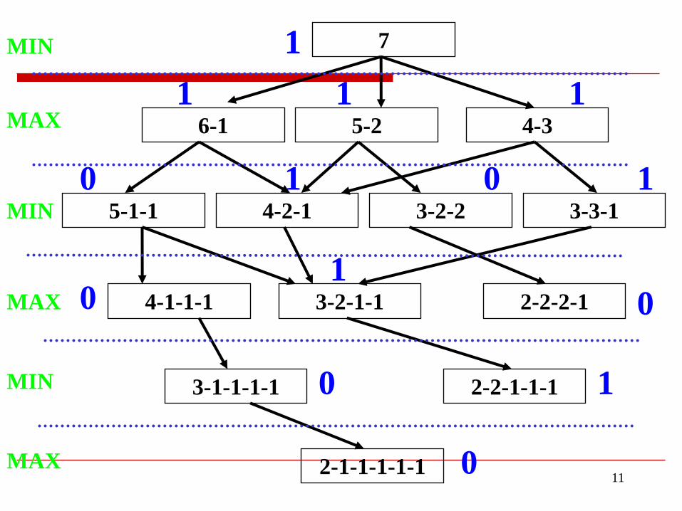
Minimax - Nim
Nim
Start with a pile of tokens
At each move the player must divide the
tokens into two non-empty, non-equal piles
++
+
10
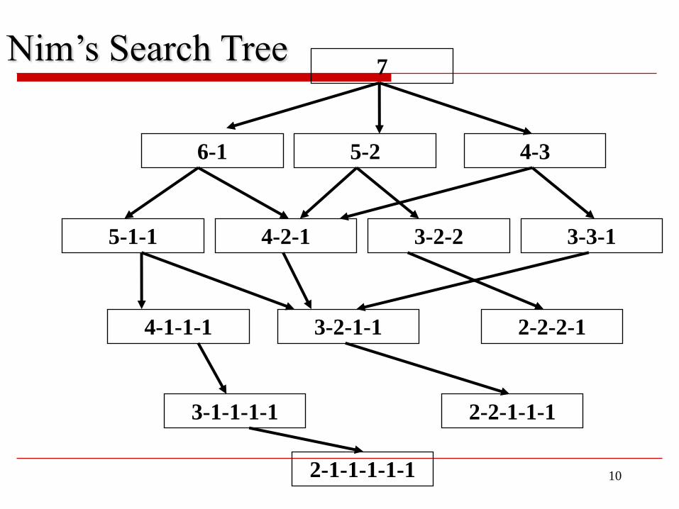
7
6-1 5-2 4-3
5-1-1 4-2-1 3-2-2 3-3-1
4-1-1-1 3-2-1-1 2-2-2-1
3-1-1-1-1 2-2-1-1-1
2-1-1-1-1-1
Nim’s Search Tree
11
7
6-1 5-2 4-3
5-1-1 4-2-1 3-2-2 3-3-1
4-1-1-1 3-2-1-1 2-2-2-1
3-1-1-1-1 2-2-1-1-1
2-1-1-1-1-1
MIN
MIN
MIN
MAX
MAX
MAX 0
1
0
0
01
0 1 0 1
1 1 1
1
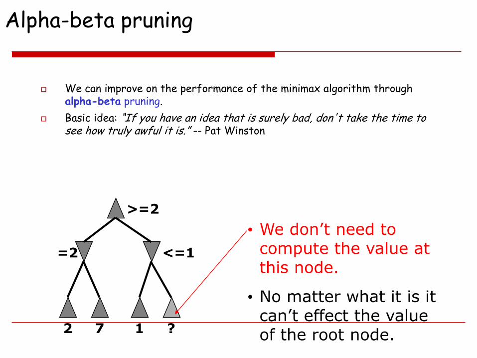
Alpha-beta pruning
We can improve on the performance of the minimax algorithm through alpha-beta pruning.
Basic idea: “If you have an idea that is surely bad, don't take the time to see how truly awful it is.” -- Pat Winston
2 7 1
=2
>=2
<=1
?
• We don’t need to compute the value at this node.
• No matter what it is it can’t effect the value of the root node.
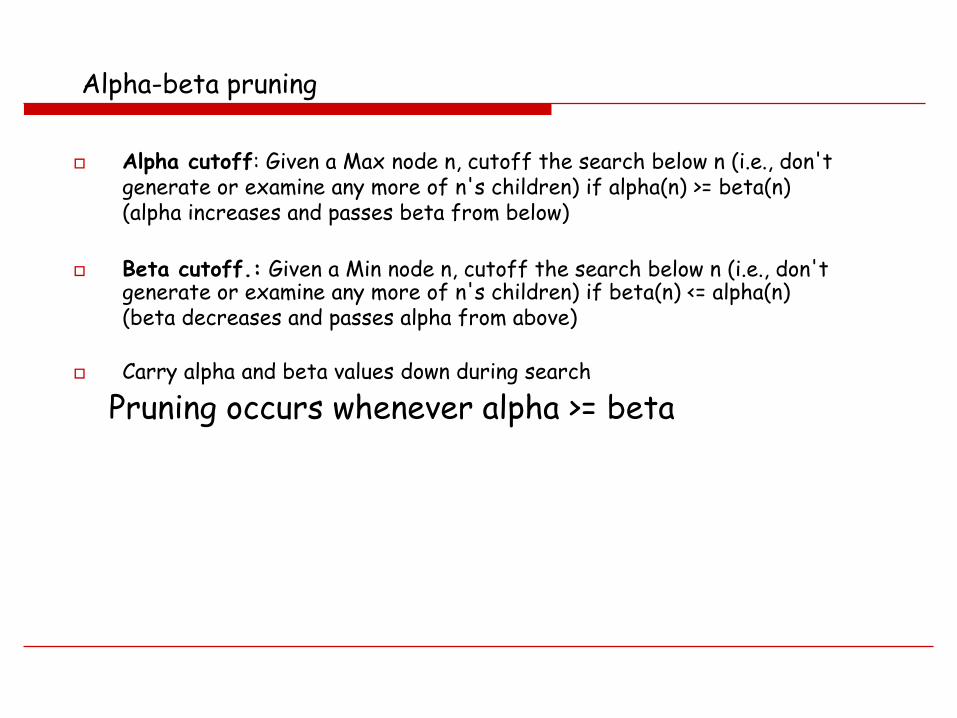
Alpha-beta pruning
Alpha cutoff: Given a Max node n, cutoff the search below n (i.e., don't generate or examine any more of n's children) if alpha(n) >= beta(n) (alpha increases and passes beta from below)
Beta cutoff.: Given a Min node n, cutoff the search below n (i.e., don't generate or examine any more of n's children) if beta(n) <= alpha(n) (beta decreases and passes alpha from above)
Carry alpha and beta values down during search
Pruning occurs whenever alpha >= beta
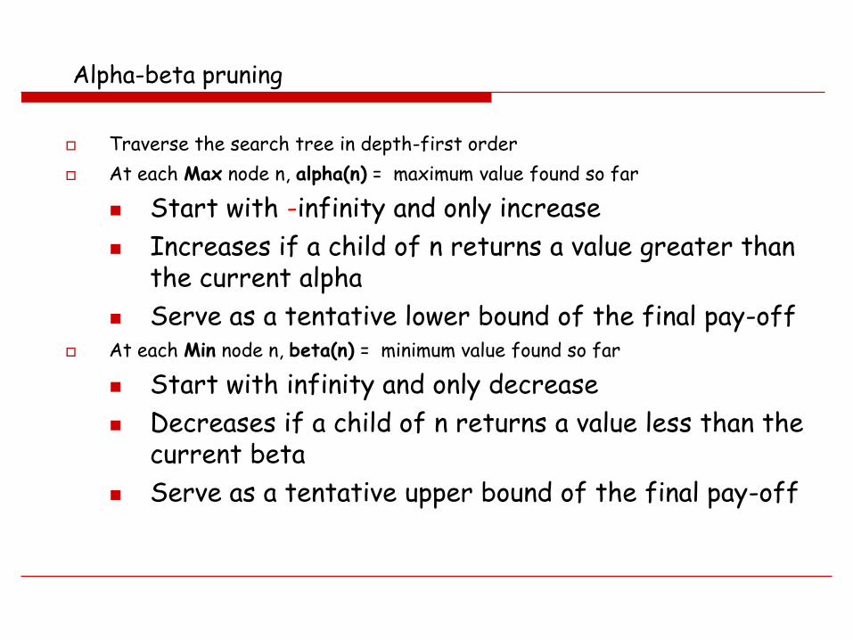
Alpha-beta pruning
Traverse the search tree in depth-first order
At each Max node n, alpha(n) = maximum value found so far
Start with -infinity and only increase
Increases if a child of n returns a value greater than the current alpha
Serve as a tentative lower bound of the final pay-off At each Min node n, beta(n) = minimum value found so far
Start with infinity and only decrease
Decreases if a child of n returns a value less than the current beta
Serve as a tentative upper bound of the final pay-off

Alpha-beta algorithm
• Two functions recursively call each other
function MAX-value (n, alpha, beta) if n is a leaf node then return f(n);for each child n’ of n do
alpha :=max{alpha, MIN-value(n’, alpha, beta)};if alpha >= beta then return beta /* pruning */
end{do}return alpha
function MIN-value (n, alpha, beta) if n is a leaf node then return f(n);for each child n’ of n do
beta :=min{beta, MAX-value(n’, alpha, beta)};if beta <= alpha then return alpha /* pruning */
end{do}return beta
:
:
:initiation
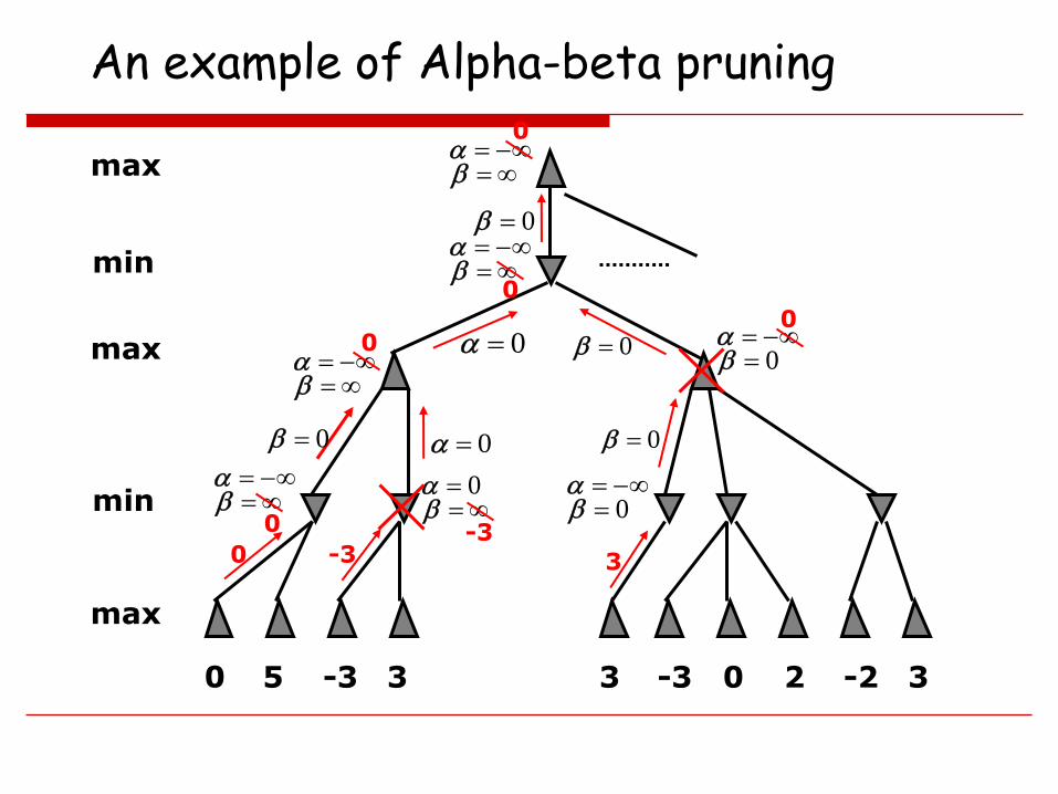
An example of Alpha-beta pruning
0 5 -3 3 3 -3 0 2 -2 3
max
max
max
min
min
0
0
0
0
0
-3
0
0 0
0
0 -3 3
0
00
0
0
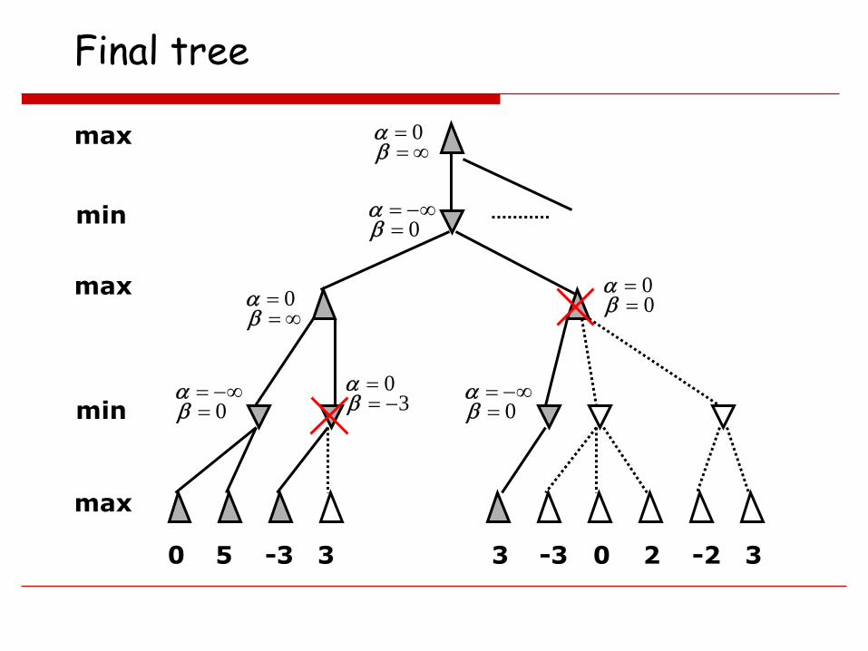
Final tree
0 5 -3 3 3 -3 0 2 -2 3
max
max
max
min
min
0
0
0
0
30
00
0
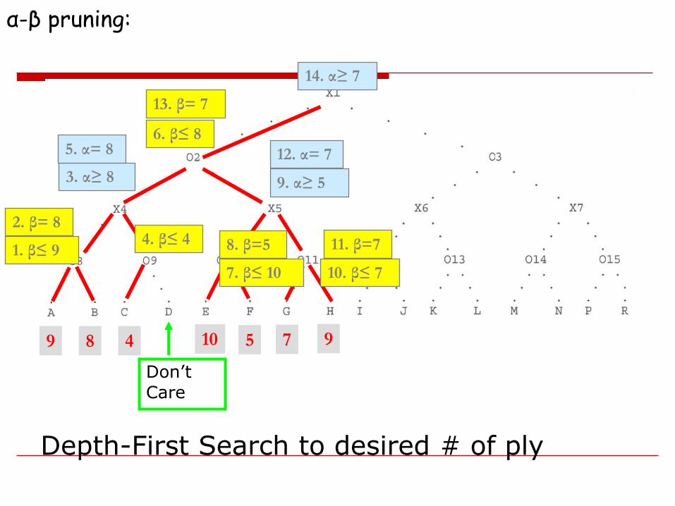
9 8 4 10 5 7 9
1. β≤ 9
2. β= 8
3. α≥ 8
4. β≤ 4
5. α= 86. β≤ 8
7. β≤ 10
8. β=5
9. α≥ 5
13. β= 7
14. α≥ 7
α-β pruning:
10. β≤ 7
11. β=7
12. α= 7
Depth-First Search to desired # of ply
Don’t
Care
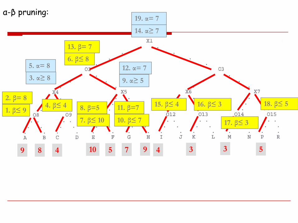
9 8 4 10 5 4 3 37 9 5
1. β≤ 9
2. β= 8
3. α≥ 8
4. β≤ 4
5. α= 86. β≤ 8
7. β≤ 10
8. β=5
9. α≥ 5
13. β= 7
14. α≥ 7
α-β pruning:
10. β≤ 7
11. β=7
12. α= 7
15. β≤ 4 16. β≤ 3
17. β≤ 3
18. β≤ 5
19. α= 7
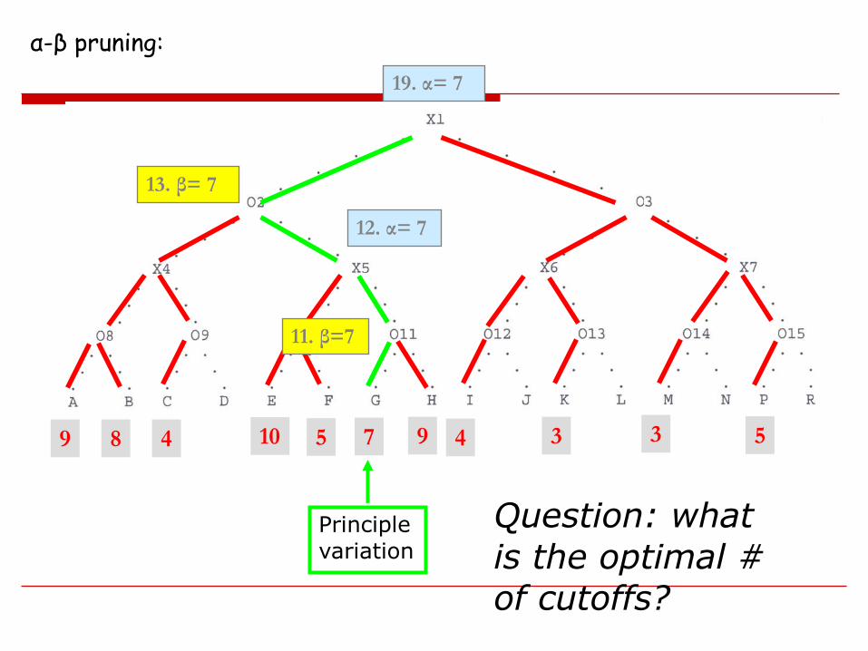
9 8 4 10 5 4 3 37 9 5
13. β= 7
α-β pruning:
11. β=7
12. α= 7
19. α= 7
Principle
variation
Question: what
is the optimal #
of cutoffs?
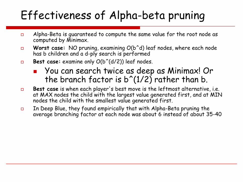
Effectiveness of Alpha-beta pruning
Alpha-Beta is guaranteed to compute the same value for the root node as computed by Minimax.
Worst case: NO pruning, examining O(b^d) leaf nodes, where each node has b children and a d-ply search is performed
Best case: examine only O(b^(d/2)) leaf nodes.
You can search twice as deep as Minimax! Or the branch factor is b^(1/2) rather than b.
Best case is when each player's best move is the leftmost alternative, i.e. at MAX nodes the child with the largest value generated first, and at MIN nodes the child with the smallest value generated first.
In Deep Blue, they found empirically that with Alpha-Beta pruning the average branching factor at each node was about 6 instead of about 35-40
E&CE 457 Applied Artificial Intelligence Page 22
Games of chance
Game of chance is anything with a random factor; e.g., dice, cards, etc.
Can extend the minimax method to handle games of chance.
This results in an expectiminimax tree.
In an expectiminimax tree, levels of max and min nodes are interleaved with "chance" nodes.
Rather than taking the max or min of the payoff values of their children, chance nodes take a weighted average (expected value) of their children.
Weights are the probability that the chance node is reached.
Each chance node gets an “expectiminimax value”.
E&CE 457 Applied Artificial Intelligence Page 23
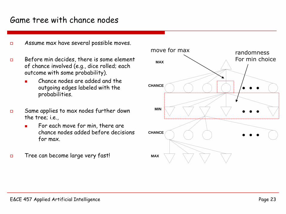
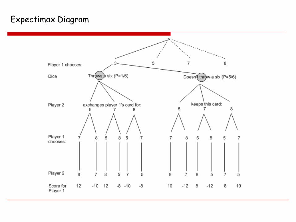
Game tree with chance nodes
Assume max have several possible moves.
Before min decides, there is some element of chance involved (e.g., dice rolled; each outcome with some probability).
Chance nodes are added and the outgoing edges labeled with the probabilities.
Same applies to max nodes further down the tree; i.e.,
For each move for min, there are chance nodes added before decisions for max.
Tree can become large very fast!
MAX
MIN
CHANCE
CHANCE
MAX
move for max randomnessFor min choice
E&CE 457 Applied Artificial Intelligence Page 24
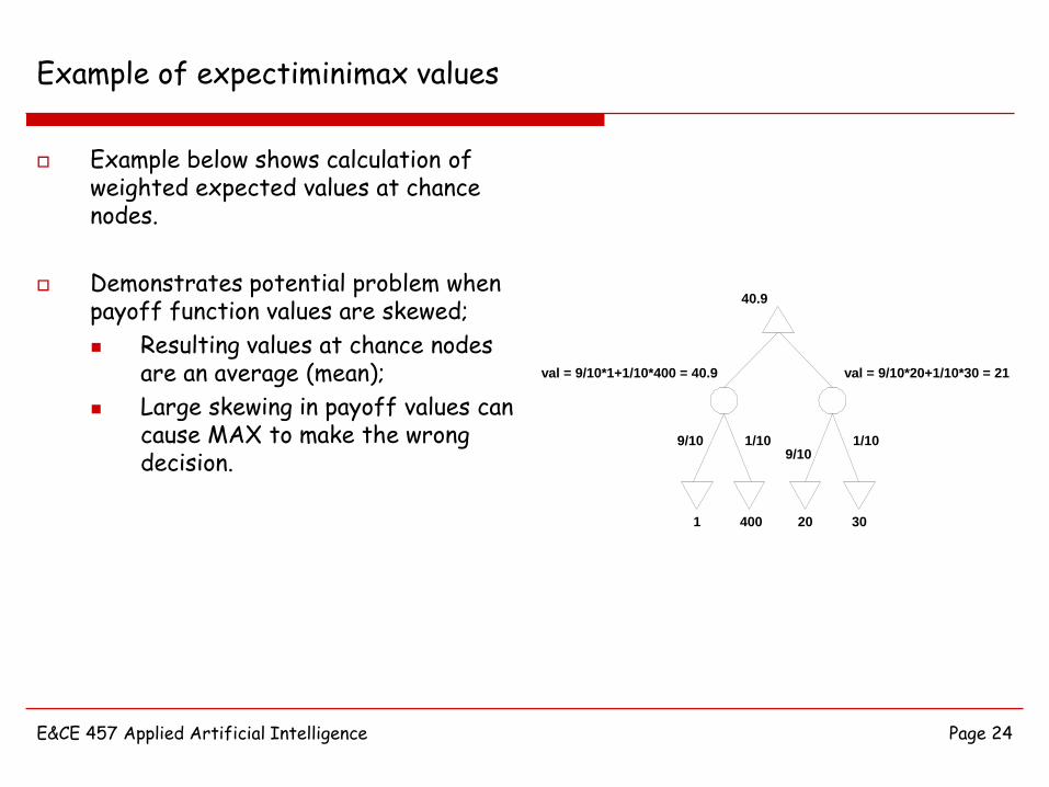
Example of expectiminimax values
Example below shows calculation of weighted expected values at chance nodes.
Demonstrates potential problem when payoff function values are skewed;
Resulting values at chance nodes are an average (mean);
Large skewing in payoff values can cause MAX to make the wrong decision.
1 400 20 30
9/101/109/10 1/10
val = 9/10*1+1/10*400 = 40.9 val = 9/10*20+1/10*30 = 21
40.9
Expectimax Diagram
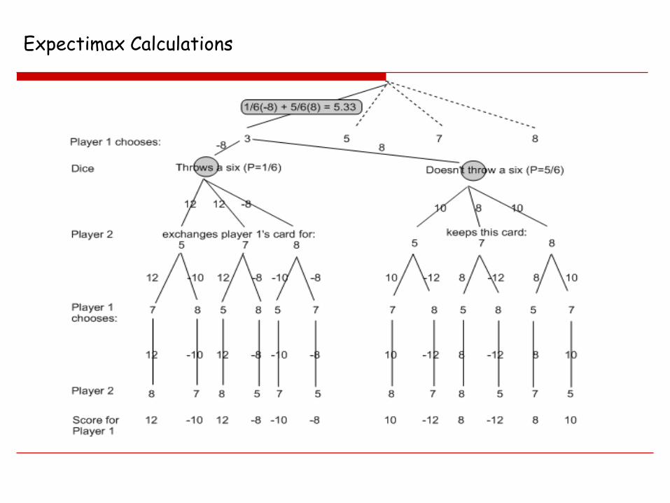
Expectimax Calculations
ECE457 Applied Artificial Intelligence Page 27
Local Search- Iterative improvement
Might have a problem in which we only care about the goal itself; path to goal is irrelevant.
Similarly, might be true that every state can be considered a goal, but has an associated cost.
We therefore have a minimization (or maximization) problem.
E.g., trying to minimize cost or maximize payoff
Can often solve such a problem as follows:
Start with an initial state/solution and modify the state/solution via actions in order to improve the quality of the state/solution.
This is known as iterative improvement
i.e., working in iterations to get closer to goal
Local search algorithms- iterative improvement
Previously: systematic exploration of search space.
Path to goal is solution to problem
Yet, for some problems path is irrelevant. In many optimization problems,
for example, the path to the goal is irrelevant; the goal state itself is the
solution
State space = set of "complete" configurations
Find configuration satisfying constraints,
e.g., n-queens problem
Local search
Can often solve such a problem as follows:
Start with an initial state/solution and modify the state/solution via actions in order to improve the quality of the state/solution.
This is known as iterative improvement
i.e., working in iterations to get closer to goal
Local search and optimization
Local search= use single current state and move to neighboring states.
Advantages:□ Uses very little memory□ Find often reasonable solutions in large or infinite state spaces.
Are also useful for pure optimization problems.□ Find best state according to some objective function.□ e.g. survival of the fittest as a metaphor for optimization.
ECE457 Applied Artificial Intelligence Page 31
Local search illustrated
Consider the 8-queens problem; goal is a board configuration w/o any attacks.
Assume a state representation in which all 8 queens are placed on the board; one queen per column:
Some states will be goal states while others are not.
Can move from state-to-state by randomly choosing a column and randomly switching the queen in the column to another row.
ECE457 Applied Artificial Intelligence Page 32
Local search illustrated
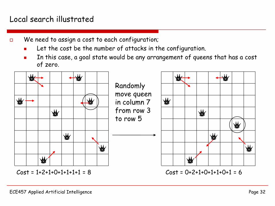
We need to assign a cost to each configuration;
Let the cost be the number of attacks in the configuration.
In this case, a goal state would be any arrangement of queens that has a cost of zero.
Cost = 1+2+1+0+1+1+1+1 = 8 Cost = 0+2+1+0+1+1+0+1 = 6
Randomly move queen in column 7 from row 3 to row 5
Elements of Local Search:
• Representation of the solution;
• Evaluation function;
• Neighbourhood function: to define solutions which can be considered close to a given solution. For example:
• For optimisation of real-valued functions in elementary calculus, for a current solution x0, neighbourhood is defined as an interval (x0 –r, x0 +r).
• In clustering problem, all the solutions which can be derived from a given solution by moving one customer from one cluster to another;
• Neighbourhood search strategy: random and systematic search;
•Acceptance criterion: first improvement, best improvement, best of non-improving solutions, random criteria;
ECE457 Applied Artificial Intelligence Page 34
Some iterative improvement strategies
We will consider several strategies:
Hill Climbing (equivalently, gradient descent),
Simulated Annealing, and
Genetic Algorithms.
In all cases, we will assume we have some sort of objective function that we would like to either minimize or maximize. (e.g., cost or payoff)
Note: sometimes when we formulate a problem such that it is solvable via iterative improvement, we need to make a decision about allowing feasible vs. infeasible solutions;
If we allow infeasible solutions, we need to augment the objective function with penalties to make infeasible solutions more costly (cf. the 8-queens problem).
ECE457 Applied Artificial Intelligence Page 35
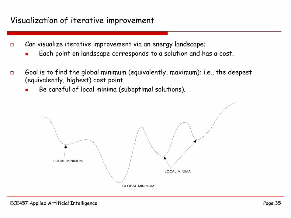
Visualization of iterative improvement
Can visualize iterative improvement via an energy landscape;
Each point on landscape corresponds to a solution and has a cost.
Goal is to find the global minimum (equivalently, maximum); i.e., the deepest (equivalently, highest) cost point.
Be careful of local minima (suboptimal solutions).
GLOBAL MINIMUM
LOCAL MINIMA
LOCAL MINIMUM
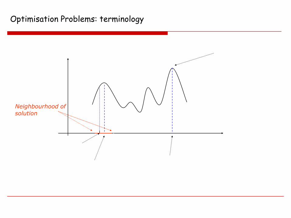
Optimisation Problems: terminology
f(X)
X
local maximum
solution
global maximum
solution
( )
Neighbourhood of
solution
global maximum
value
Y
ECE457 Applied Artificial Intelligence Page 37
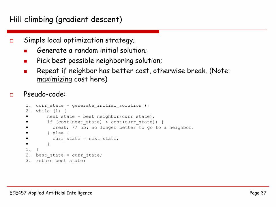
Hill climbing (gradient descent)
Simple local optimization strategy;
Generate a random initial solution;
Pick best possible neighboring solution;
Repeat if neighbor has better cost, otherwise break. (Note: maximizing cost here)
Pseudo-code:
1. curr_state = generate_initial_solution();
2. while (1) {
• next_state = best_neighbor(curr_state);
• if (cost(next_state) < cost(curr_state)) {
• break; // nb: no longer better to go to a neighbor.
• } else {
• curr_state = next_state;
• }
1. }
2. best_state = curr_state;
3. return best_state;
ECE457 Applied Artificial Intelligence Page 38
Hill climbing (gradient descent)
Advantages;
No search trees;
Typically very fast (if neighbor generation and evaluation is fast).
Disadvantages:
Final solution found subject to initial solution.
Can get stuck in a local, sub-optimal solution. Does not look beyond immediate neighbors
Does not allow worse moves
This method is very much a localized improvement strategy.
Common to use this approach with either;
Many random initial solutions (multi-starts), or
Some intelligently constructed initial solution (from another method).
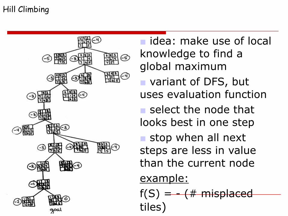
Hill Climbing
■ idea: make use of local
knowledge to find a
global maximum
■ variant of DFS, but
uses evaluation function
■ select the node that
looks best in one step
■ stop when all next
steps are less in value
than the current node
example:
f(S) = - (# misplaced
tiles)
Hill-climbing example
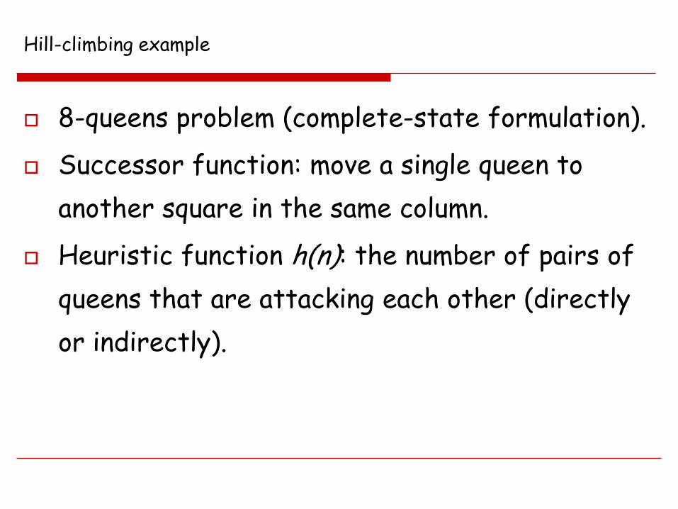
8-queens problem (complete-state formulation).
Successor function: move a single queen to
another square in the same column.
Heuristic function h(n): the number of pairs of
queens that are attacking each other (directly
or indirectly).
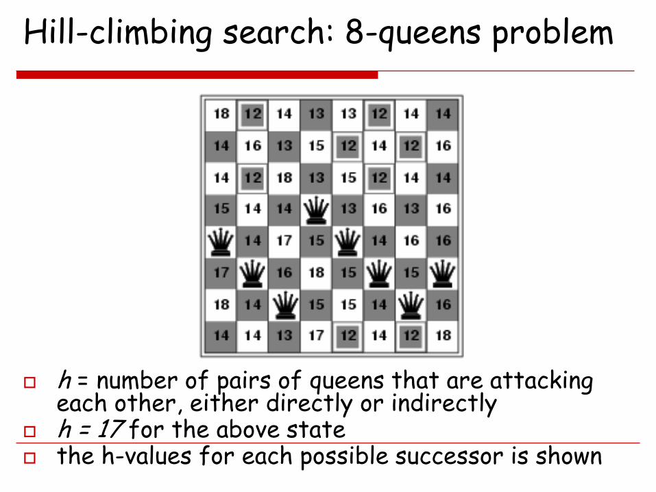
Hill-climbing search: 8-queens problem
h = number of pairs of queens that are attacking each other, either directly or indirectly
h = 17 for the above state the h-values for each possible successor is shown
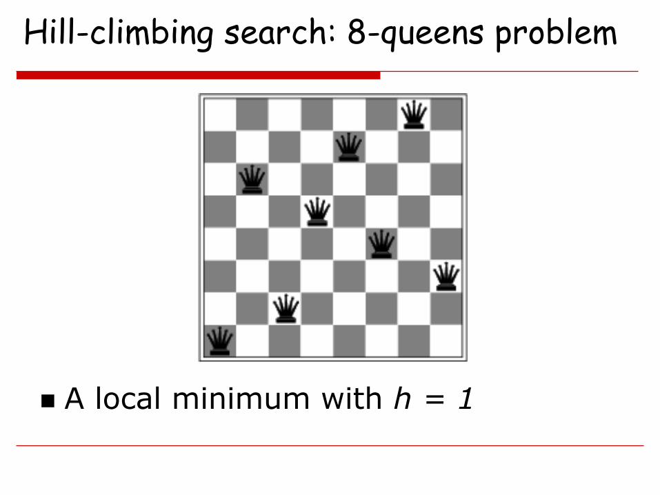
Hill-climbing search: 8-queens problem
A local minimum with h = 1
ECE457 Applied Artificial Intelligence Page 43
Simulated Annealing
Problem with hill climbing: local best move doesn’t lead to optimal goal
Solution: allow bad moves
Simulated annealing is a popular way of doing that
Stochastic search method
Simulates annealing process in metallurgy
ECE457 Applied Artificial Intelligence Page 44
Annealing
Tempering technique in metallurgy
Weakness and defects come from atoms of crystals freezing in the wrong place
(local optimum)
Heating to unstuck the atoms (escape local optimum)
Slow cooling to allow atoms to get to better place (global optimum)
ECE457 Applied Artificial Intelligence R. Khoury (2008) Page 45
Simulated Annealing
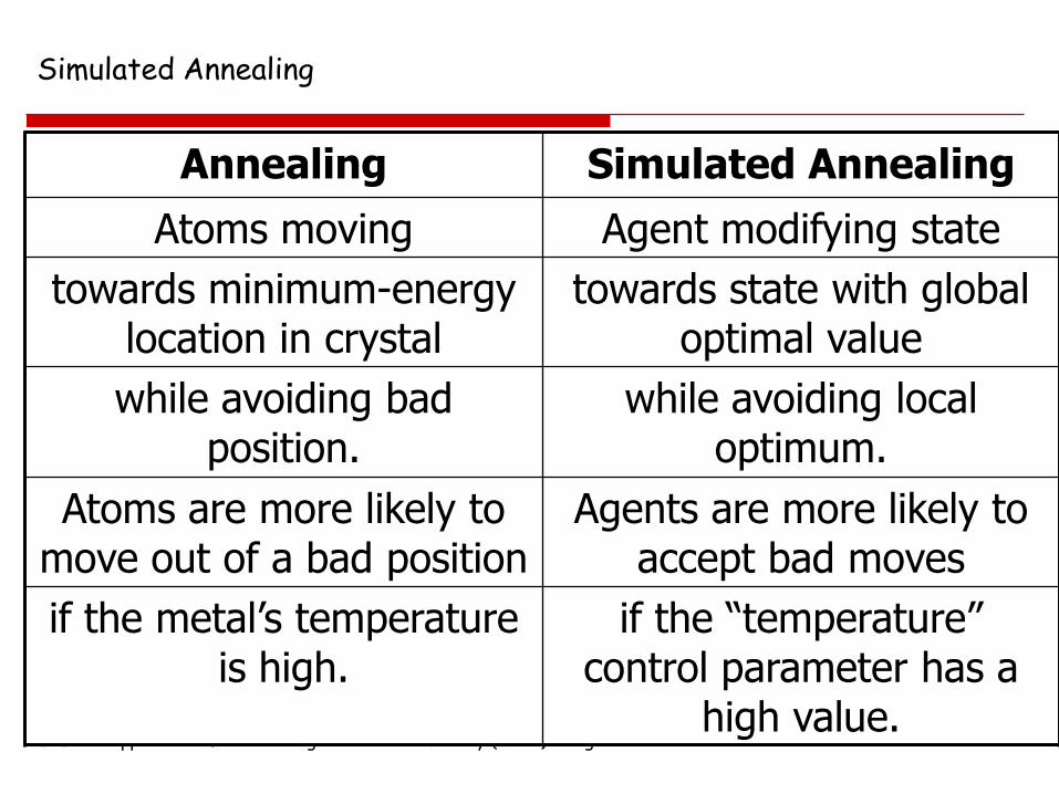
Annealing Simulated Annealing
Atoms moving Agent modifying state
towards minimum-energy location in crystal
towards state with global optimal value
while avoiding bad position.
while avoiding local optimum.
Atoms are more likely to move out of a bad position
Agents are more likely to accept bad moves
if the metal’s temperature is high.
if the “temperature” control parameter has a
high value.
ECE457 Applied Artificial Intelligence Page 46
Simulated Annealing
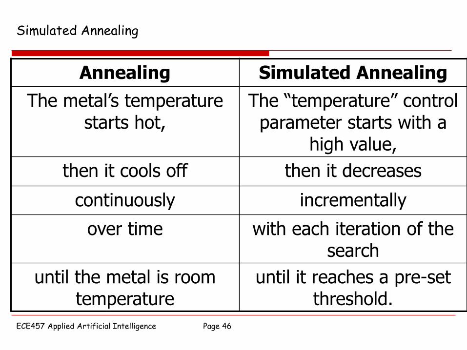
Annealing Simulated Annealing
The metal’s temperature starts hot,
The “temperature” control parameter starts with a
high value,
then it cools off then it decreases
continuously incrementally
over time with each iteration of the search
until the metal is room temperature
until it reaches a pre-set threshold.
ECE457 Applied Artificial Intelligence Page 47
Simulated Annealing
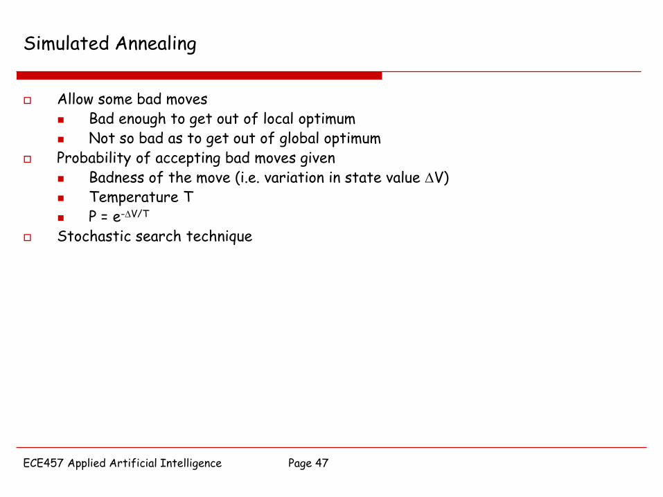
Allow some bad moves Bad enough to get out of local optimum Not so bad as to get out of global optimum
Probability of accepting bad moves given Badness of the move (i.e. variation in state value V) Temperature T P = e-V/T
Stochastic search technique
ECE457 Applied Artificial Intelligence Page 48
Simulated Annealing
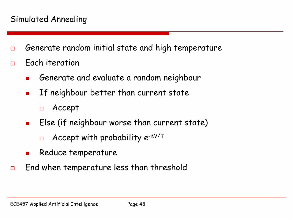
Generate random initial state and high temperature
Each iteration
Generate and evaluate a random neighbour
If neighbour better than current state
Accept
Else (if neighbour worse than current state)
Accept with probability e-V/T
Reduce temperature
End when temperature less than threshold
ECE457 Applied Artificial Intelligence Page 49
Simulated Annealing
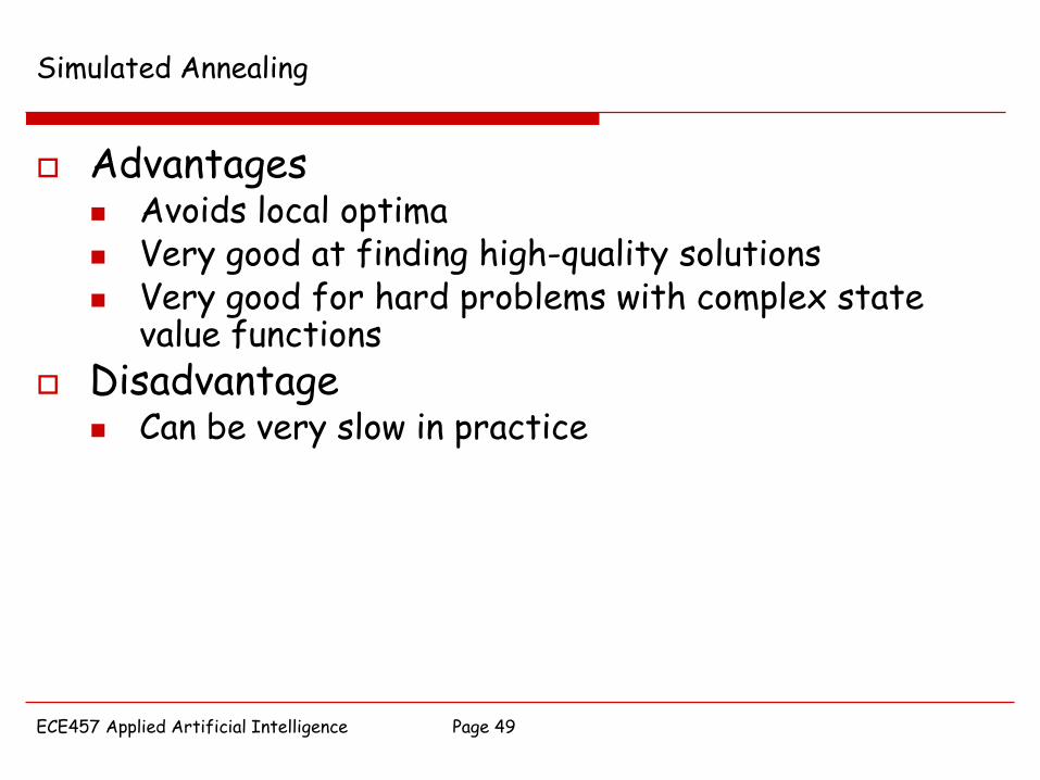
Advantages Avoids local optima Very good at finding high-quality solutions Very good for hard problems with complex state
value functions
Disadvantage Can be very slow in practice
Simulated Annealing
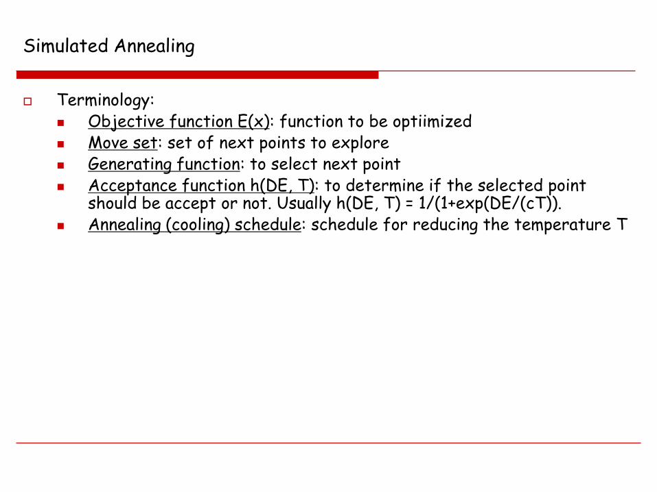
Terminology: Objective function E(x): function to be optiimized Move set: set of next points to explore Generating function: to select next point Acceptance function h(DE, T): to determine if the selected point
should be accept or not. Usually h(DE, T) = 1/(1+exp(DE/(cT)). Annealing (cooling) schedule: schedule for reducing the temperature T
Simulated Annealing
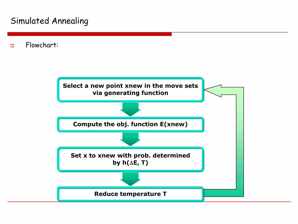
Flowchart:
Select a new point xnew in the move sets
via generating function
Compute the obj. function E(xnew)
Set x to xnew with prob. determined
by h(E, T)
Reduce temperature T
ECE457 Applied Artificial Intelligence Page 52
Accepting moves in simulated annealing
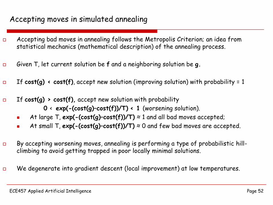
Accepting bad moves in annealing follows the Metropolis Criterion; an idea from statistical mechanics (mathematical description) of the annealing process.
Given T, let current solution be f and a neighboring solution be g.
If cost(g) < cost(f), accept new solution (improving solution) with probability = 1
If cost(g) > cost(f), accept new solution with probability
0 < exp(-(cost(g)–cost(f))/T) < 1 (worsening solution).
At large T, exp(-(cost(g)–cost(f))/T) ≈ 1 and all bad moves accepted;
At small T, exp(-(cost(g)–cost(f))/T) ≈ 0 and few bad moves are accepted.
By accepting worsening moves, annealing is performing a type of probabilistic hill-climbing to avoid getting trapped in poor locally minimal solutions.
We degenerate into gradient descent (local improvement) at low temperatures.
ECE457 Applied Artificial Intelligence Page 53
Pseudo-code for simulated annealing
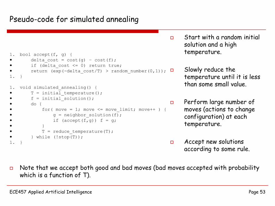
Start with a random initial solution and a high temperature.
Slowly reduce the temperature until it is less than some small value.
Perform large number of moves (actions to change configuration) at each temperature.
Accept new solutions according to some rule.
1. bool accept(f, g) {
• delta_cost = cost(g) – cost(f);
• if (delta_cost <= 0) return true;
• return (exp(-delta_cost/T) > random_number(0,1));
1. }
1. void simulated_annealing() {
• T = initial_temperature();
• f = initial_solution();
• do {
• for( move = 1; move <= move_limit; move++ ) {
• g = neighbor_solution(f);
• if (accept(f,g)) f = g;
• }
• T = reduce_temperature(T);
• } while (!stop(T));
1. }
Note that we accept both good and bad moves (bad moves accepted with probability which is a function of T).
ECE457 Applied Artificial Intelligence Page 54
Illustration of cost and acceptance during simulated annealing
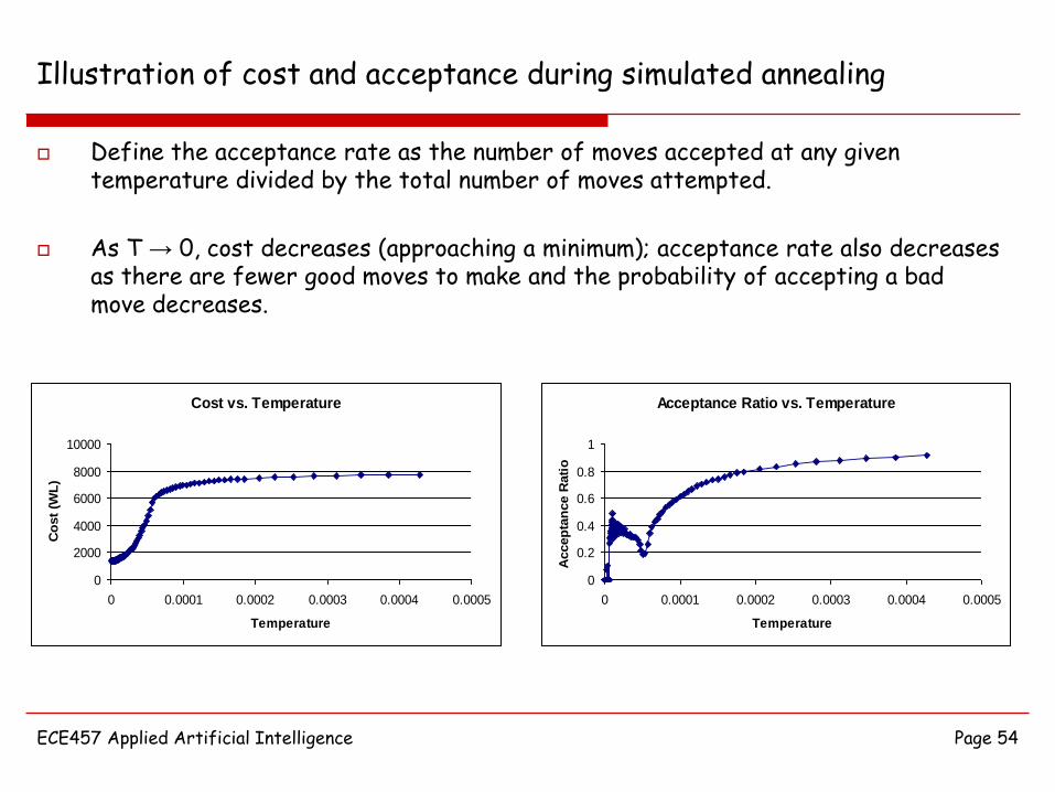
Define the acceptance rate as the number of moves accepted at any given temperature divided by the total number of moves attempted.
As T → 0, cost decreases (approaching a minimum); acceptance rate also decreases as there are fewer good moves to make and the probability of accepting a bad move decreases.
Cost vs. Temperature
0
2000
4000
6000
8000
10000
0 0.0001 0.0002 0.0003 0.0004 0.0005
Temperature
Co
st
(WL
)
Acceptance Ratio vs. Temperature
0
0.2
0.4
0.6
0.8
1
0 0.0001 0.0002 0.0003 0.0004 0.0005
Temperature
Accep
tan
ce R
ati
o
ECE457 Applied Artificial Intelligence Page 55
Simulated annealing
Advantages:
Avoids local minima since worsening moves allowed.
Popular algorithm for hard problems with complicated cost functions.
Works really well at finding good, high quality solutions.
There is a theoretical proof of convergence (asymptotic), so somewhat useless in practice.
Disadvantages:
Can be very slow in practice since lots of moves are performed.
ECE457 Applied Artificial Intelligence Page 56
Illustration of simulated annealing for fpga placement
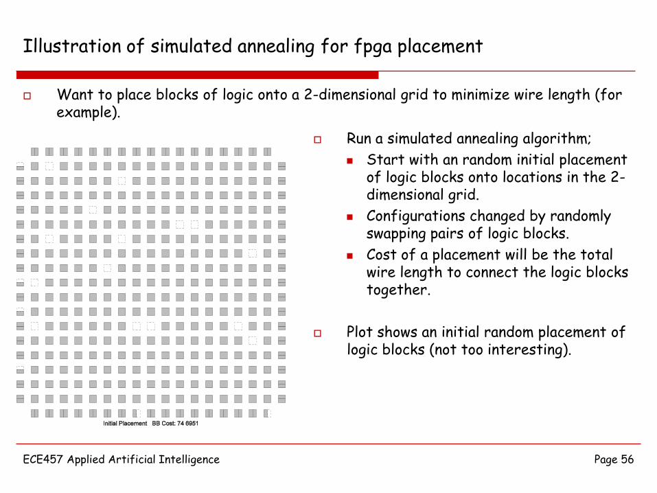
Want to place blocks of logic onto a 2-dimensional grid to minimize wire length (for example).
Run a simulated annealing algorithm;
Start with an random initial placement of logic blocks onto locations in the 2-dimensional grid.
Configurations changed by randomly swapping pairs of logic blocks.
Cost of a placement will be the total wire length to connect the logic blocks together.
Plot shows an initial random placement of logic blocks (not too interesting).
ECE457 Applied Artificial Intelligence Page 57
Illustration of simulated annealing for fpga placement
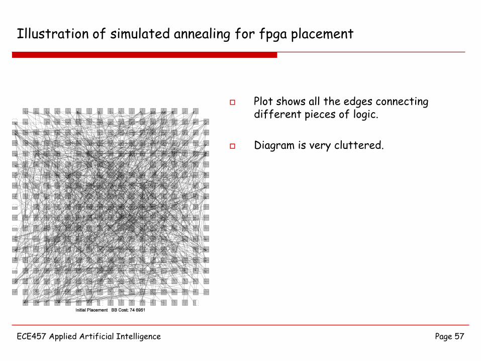
Plot shows all the edges connecting different pieces of logic.
Diagram is very cluttered.
ECE457 Applied Artificial Intelligence Page 58
Illustration of simulated annealing for fpga placement
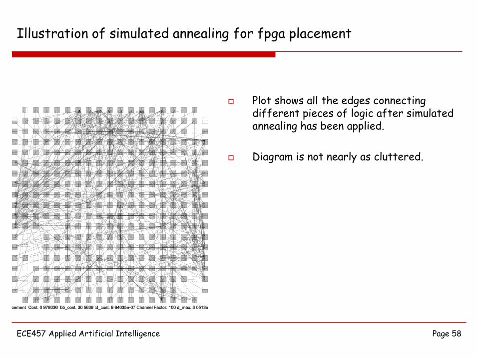
Plot shows all the edges connecting different pieces of logic after simulated annealing has been applied.
Diagram is not nearly as cluttered.
ECE457 Applied Artificial Intelligence Page 59
Illustration of simulated annealing for fpga placement
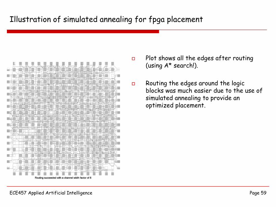
Plot shows all the edges after routing (using A* search!).
Routing the edges around the logic blocks was much easier due to the use of simulated annealing to provide an optimized placement.
E&CE457 Applied Artificial Intelligence Page 60
Evolutionary Computing
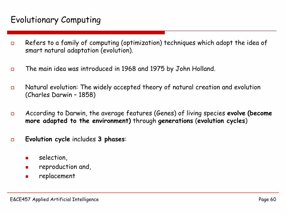
Refers to a family of computing (optimization) techniques which adopt the idea of smart natural adaptation (evolution).
The main idea was introduced in 1968 and 1975 by John Holland.
Natural evolution: The widely accepted theory of natural creation and evolution (Charles Darwin – (1858
According to Darwin, the average features (Genes) of living species evolve (become more adapted to the environment) through generations (evolution cycles)
Evolution cycle includes 3 phases:
selection,
reproduction and,
replacement
E&CE457 Applied Artificial Intelligence Page 61
Evolutionary Computing
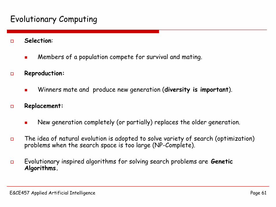
Selection:
Members of a population compete for survival and mating.
Reproduction:
Winners mate and produce new generation (diversity is important).
Replacement:
New generation completely (or partially) replaces the older generation.
The idea of natural evolution is adopted to solve variety of search (optimization) problems when the search space is too large (NP-Complete).
Evolutionary inspired algorithms for solving search problems are Genetic Algorithms.
E&CE457 Applied Artificial Intelligence Page 62
Evolutionary Computing
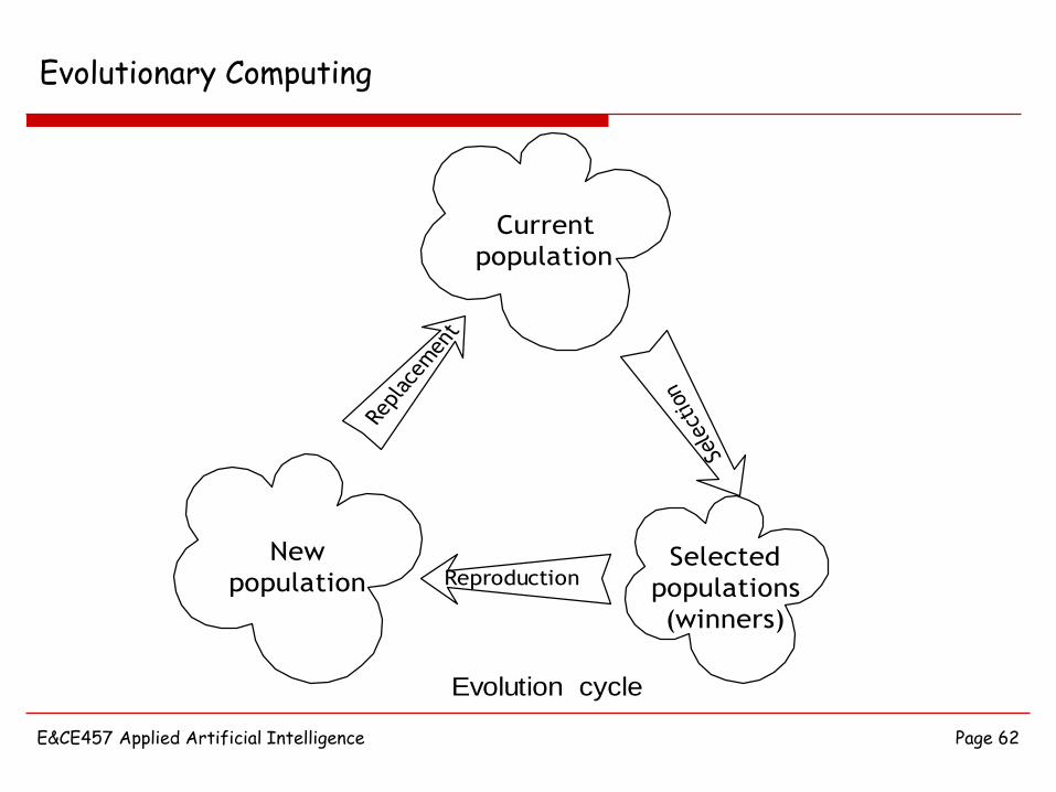
Current
population
New
populationSelected
populations
(winners)
Reproduction
Replacem
ent
Selection
Evolution cycle
E&CE457 Applied Artificial Intelligence Page 63
Genetic Algorithm Preliminaries (Fitness Functions)
Some preliminary steps are required.
Need to be able to evaluate the fitness of members of the population. Can use a fitness function.
The fitness function measures the quality of a problem solution (bigger fitness is better).
Hence, when we talk about survival, mating, etc. the idea is that new generations are (overall) more fit than older generations.
E&CE457 Applied Artificial Intelligence Page 64
Genetic Algorithm Preliminaries (Chromosome Encoding)
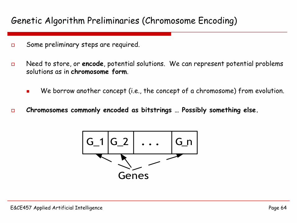
Some preliminary steps are required.
Need to store, or encode, potential solutions. We can represent potential problems solutions as in chromosome form.
We borrow another concept (i.e., the concept of a chromosome) from evolution.
Chromosomes commonly encoded as bitstrings … Possibly something else.
G_1 G_2 G_n. . .
Genes
E&CE457 Applied Artificial Intelligence Page 65
Genetic Algorithms (Main Algorithmic Steps)
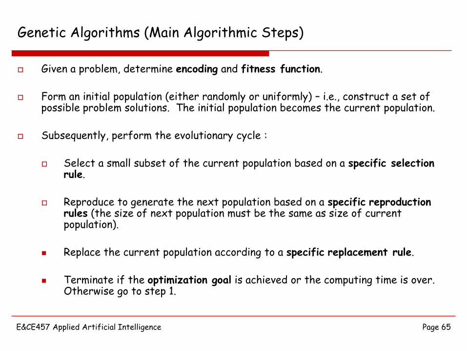
Given a problem, determine encoding and fitness function.
Form an initial population (either randomly or uniformly) – i.e., construct a set of possible problem solutions. The initial population becomes the current population.
Subsequently, perform the evolutionary cycle :
Select a small subset of the current population based on a specific selection rule.
Reproduce to generate the next population based on a specific reproduction rules (the size of next population must be the same as size of current population).
Replace the current population according to a specific replacement rule.
Terminate if the optimization goal is achieved or the computing time is over. Otherwise go to step 1.
E&CE457 Applied Artificial Intelligence Page 66
Example Problem (1 of 7)
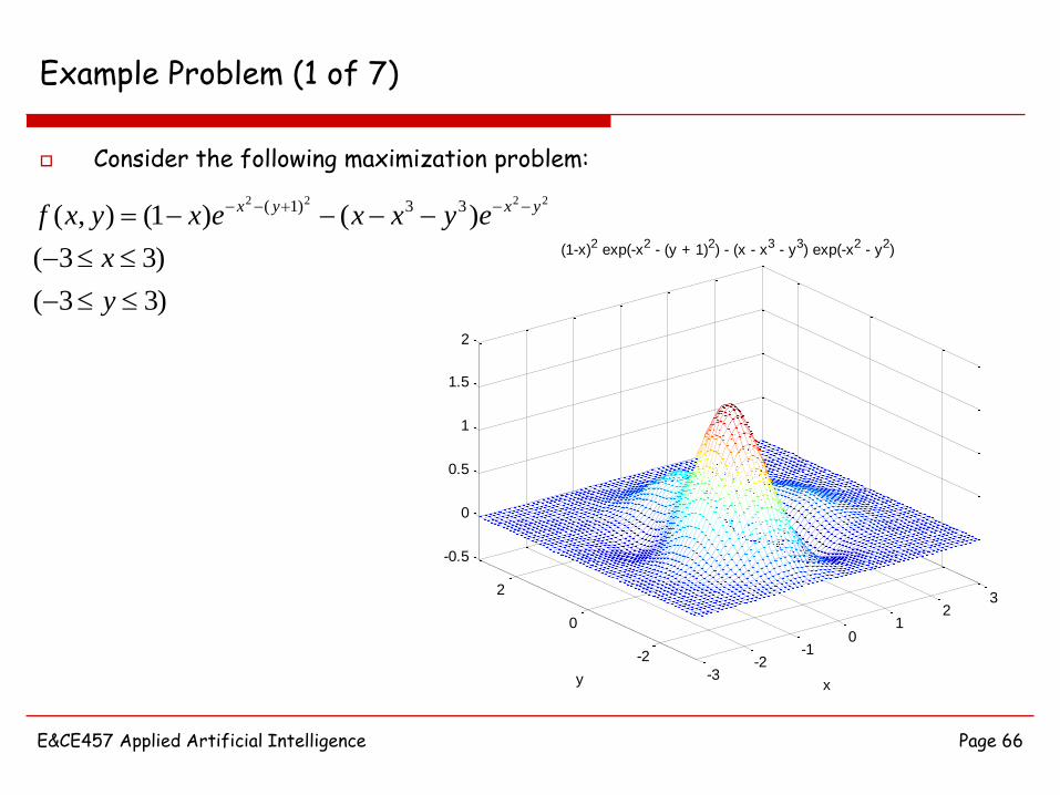
Consider the following maximization problem:
)33(
)33(
)()1(),(2222 33)1(
y
x
eyxxexyxf yxyx
-3-2
-10
12
3
-2
0
2
-0.5
0
0.5
1
1.5
2
x
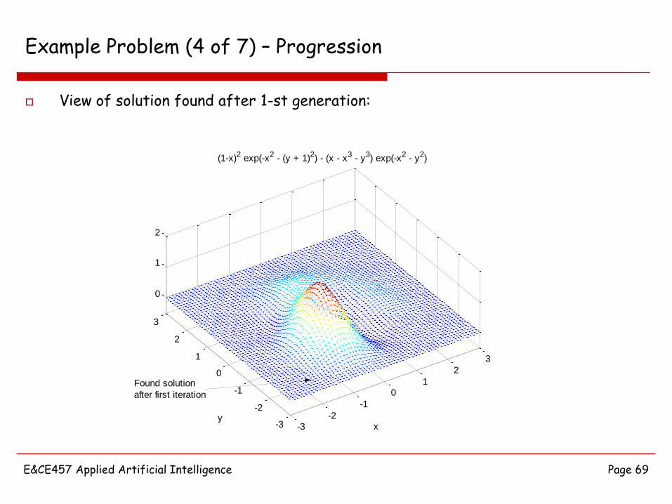
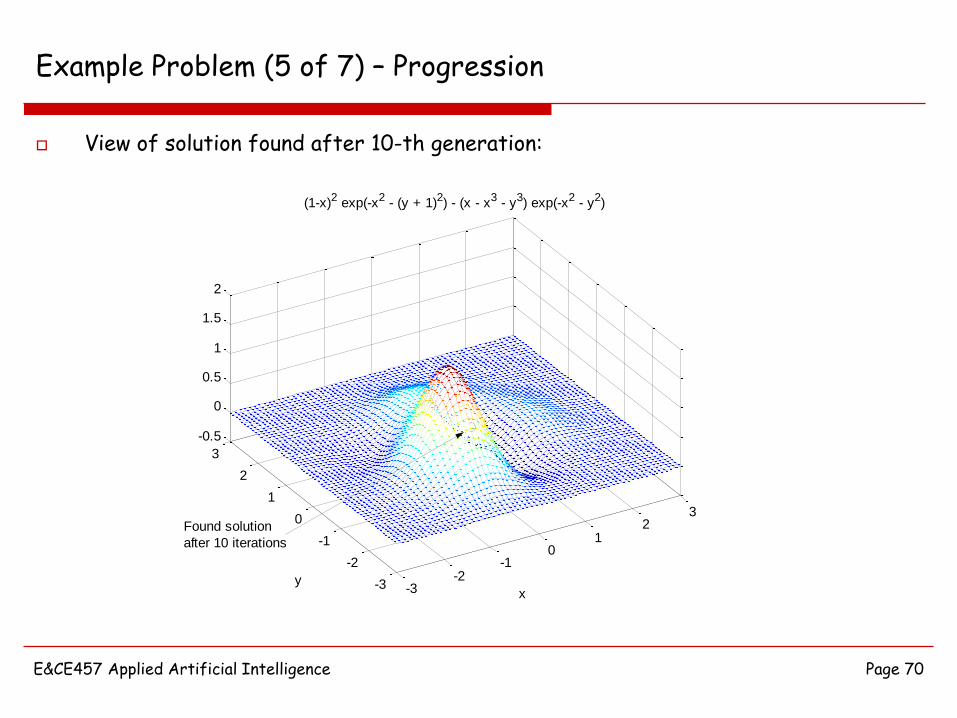
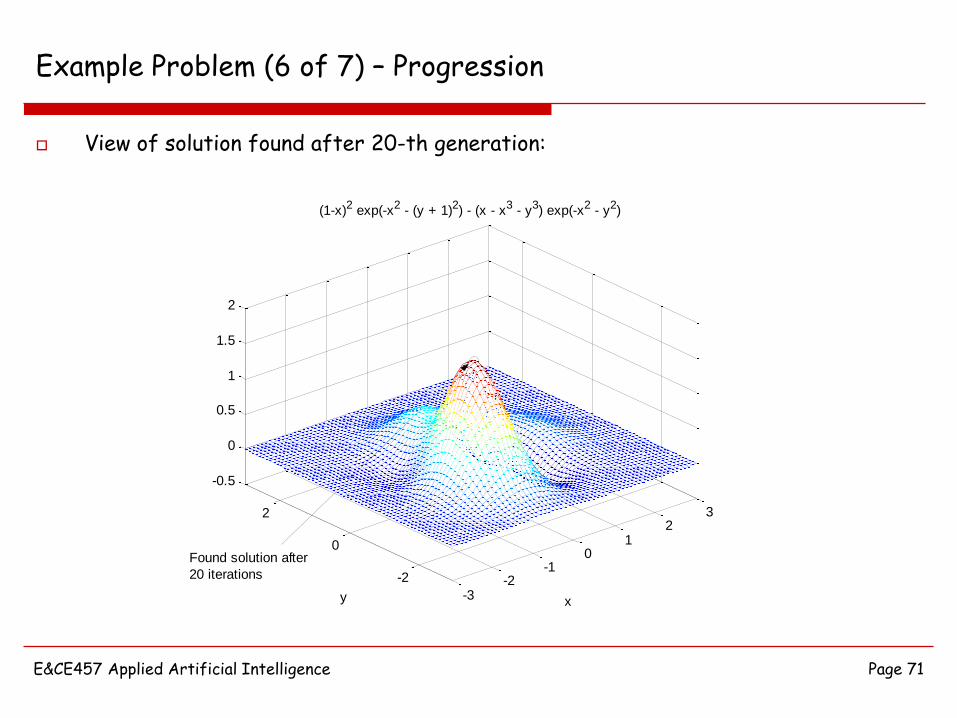
(1-x)2 exp(-x2 - (y + 1)2) - (x - x3 - y3) exp(-x2 - y2)
y
E&CE457 Applied Artificial Intelligence Page 67
Example Problem (2 of 7)
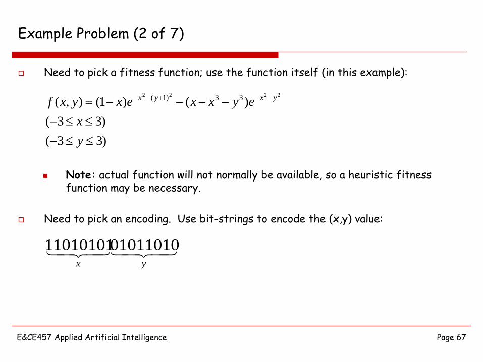
Need to pick a fitness function; use the function itself (in this example):
yx
0101101011010101
)33(
)33(
)()1(),(2222 33)1(
y
x
eyxxexyxf yxyx
Note: actual function will not normally be available, so a heuristic fitness function may be necessary.
Need to pick an encoding. Use bit-strings to encode the (x,y) value:
E&CE457 Applied Artificial Intelligence Page 68
Example Problem (3 of 7)
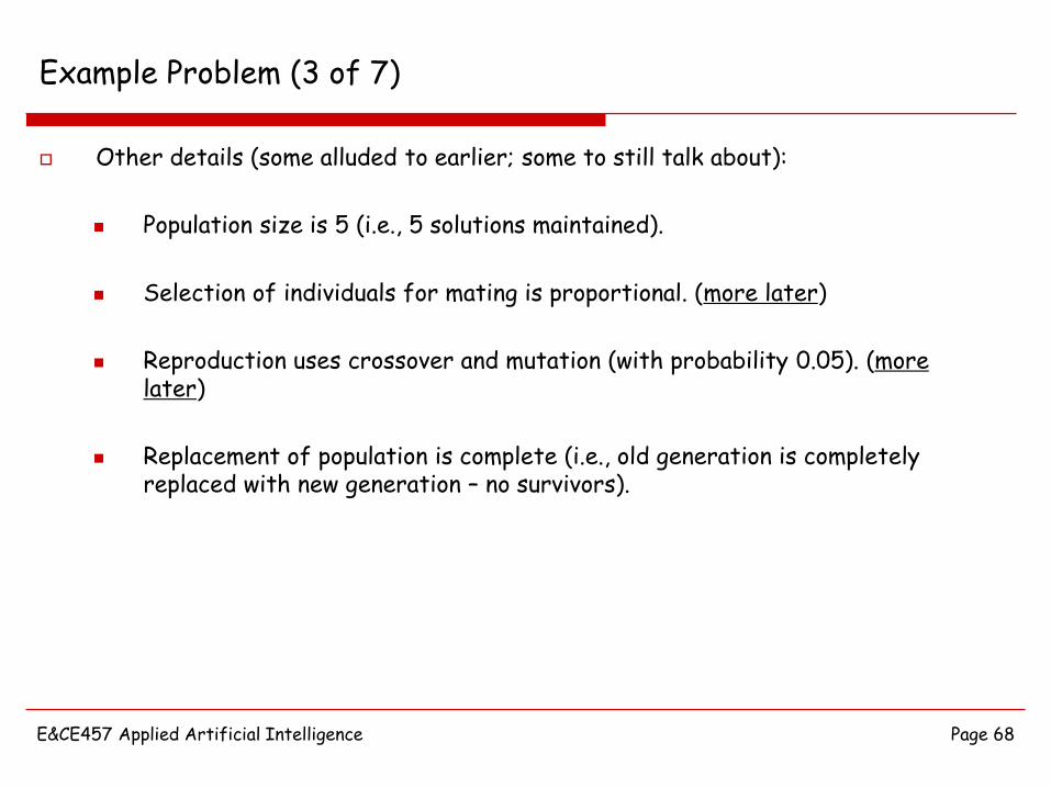
Other details (some alluded to earlier; some to still talk about):
Population size is 5 (i.e., 5 solutions maintained).
Selection of individuals for mating is proportional. (more later)
Reproduction uses crossover and mutation (with probability 0.05). (more later)
Replacement of population is complete (i.e., old generation is completely replaced with new generation – no survivors).
E&CE457 Applied Artificial Intelligence Page 69
Example Problem (4 of 7) – Progression
-3-2
-1
01
2
3
-3
-2
-1
0
1
2
3
0
1
2
x
(1-x)2 exp(-x2 - (y + 1)2) - (x - x3 - y3) exp(-x2 - y2)
y
Found solution
after first iteration
View of solution found after 1-st generation:
E&CE457 Applied Artificial Intelligence Page 70
Example Problem (5 of 7) – Progression
-3-2
-10
12
3
-3
-2
-1
0
1
2
3
-0.5
0
0.5
1
1.5
2
x
(1-x)2 exp(-x2 - (y + 1)2) - (x - x3 - y3) exp(-x2 - y2)
y
Found solution
after 10 iterations
View of solution found after 10-th generation:
E&CE457 Applied Artificial Intelligence Page 71
Example Problem (6 of 7) – Progression
-3-2
-10
12
3
-2
0
2
-0.5
0
0.5
1
1.5
2
x
(1-x)2 exp(-x2 - (y + 1)2) - (x - x3 - y3) exp(-x2 - y2)
y
Found solution after
20 iterations
View of solution found after 20-th generation:
E&CE457 Applied Artificial Intelligence Page 72
Example Problem (7 of 7)
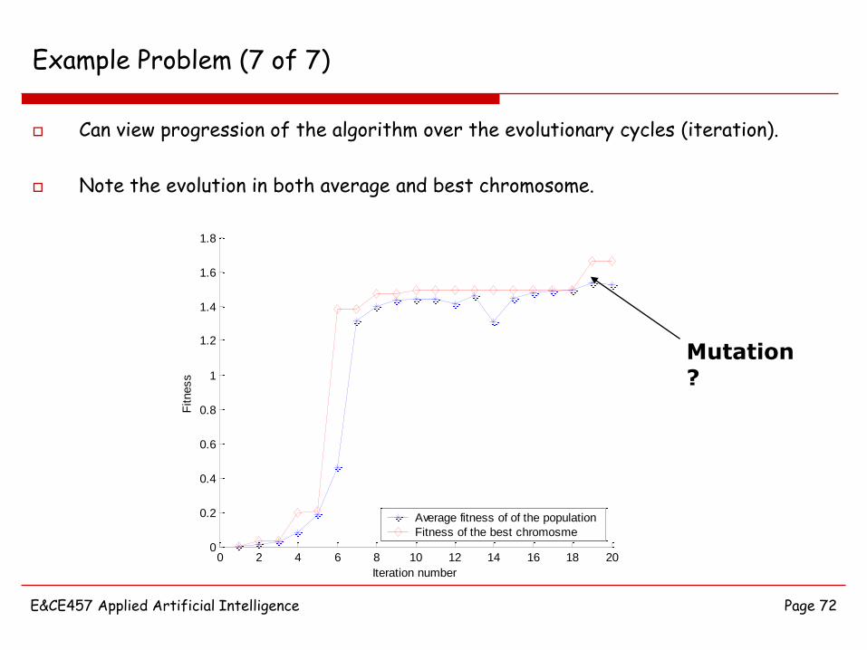
Can view progression of the algorithm over the evolutionary cycles (iteration).
Note the evolution in both average and best chromosome.
0 2 4 6 8 10 12 14 16 18 200
0.2
0.4
0.6
0.8
1
1.2
1.4
1.6
1.8
Iteration number
Fitness
Average fitness of of the population
Fitness of the best chromosme
Mutation?
E&CE457 Applied Artificial Intelligence Page 73
Selection Rules (1 of 2)
We need to pick members of the current population for reproduction (all members of population contest for reproduction).
A selection rule basically is a competition rule which gives more chance to the chromosomes with better fitness.
Chance of each chromosome (member) being selected depends on its fitness. This dependency could be:
Proportional
Exponential (greedy – emphasizes higher fitness)
Having calculated the chance of selecting each chromosome, a roulette wheel scheme could be used to select required number of selected generations.
E&CE457 Applied Artificial Intelligence Page 74
Selection Rules (2 of 2)*
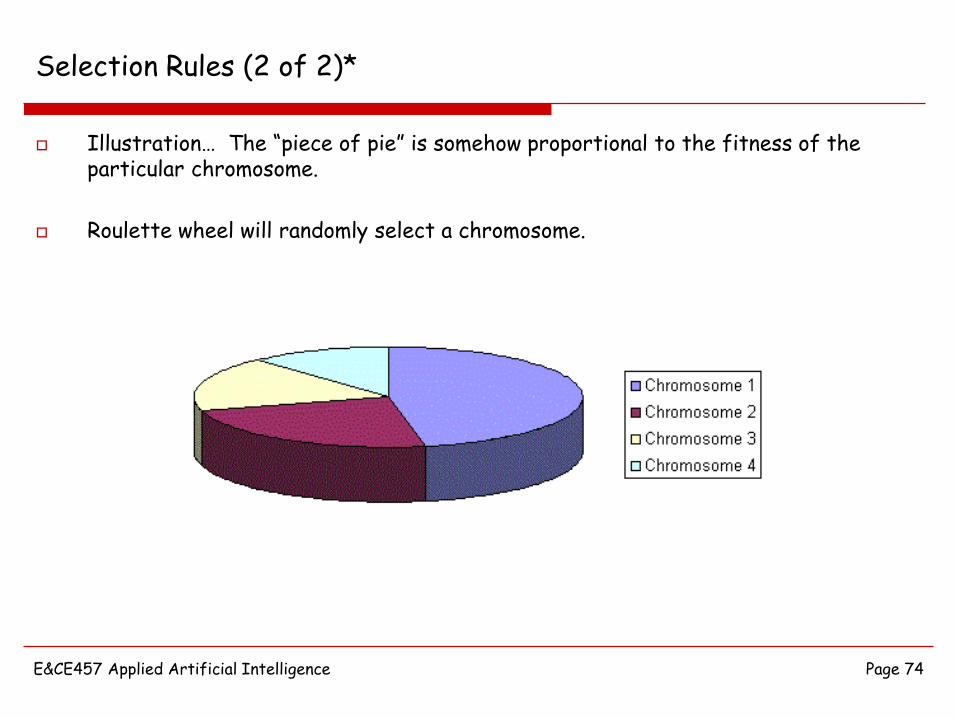
Illustration… The “piece of pie” is somehow proportional to the fitness of the particular chromosome.
Roulette wheel will randomly select a chromosome.
E&CE457 Applied Artificial Intelligence Page 75
Reproduction Rules (1 of 3)
Once we have selected two members, we need to use them for reproduction.
Generally, a good reproduction rule should create good DIVERSITY in the new population.
Idea is to help improve the exploration of the search space.
Well known techniques for reproduction (to achieve diversity):
Crossover.
Mutation.
E&CE457 Applied Artificial Intelligence Page 76
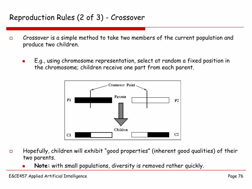
Reproduction Rules (2 of 3) - Crossover
Crossover is a simple method to take two members of the current population and produce two children.
E.g., using chromosome representation, select at random a fixed position in the chromosome; children receive one part from each parent.
Hopefully, children will exhibit “good properties” (inherent good qualities) of their two parents.
Note: with small populations, diversity is removed rather quickly.
E&CE457 Applied Artificial Intelligence Page 77
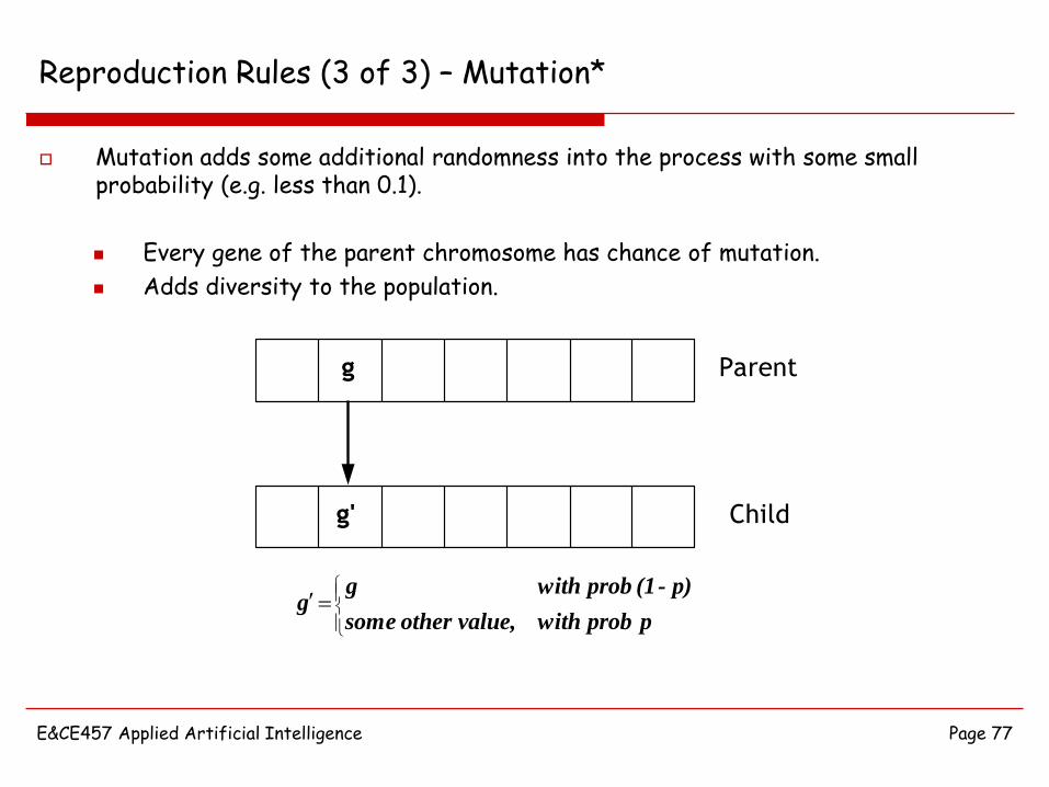
Reproduction Rules (3 of 3) – Mutation*
Mutation adds some additional randomness into the process with some small probability (e.g. less than 0.1).
Every gene of the parent chromosome has chance of mutation.
Adds diversity to the population.
Parent
Child
g
g'
p prob withvalue, othersome
p)-(1 prob withgg
E&CE457 Applied Artificial Intelligence Page 78
Replacement Rules
Must decide (given current population and produced children), how to form the new population.
In most existing variants of GA, the number of individuals in the next population is the same as current population.
Different replacement schemes:
Whole replacement of current population with the reproduced population.
Individuals with the best fitness from the current and reproduced population are chosen to make new population (greedy approach).
Being greedy (can) compromise the exploration capability of the algorithm (premature convergence).
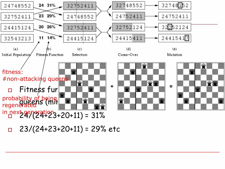
Fitness function: number of non-attacking pairs of
queens (min = 0, max = 8 × 7/2 = 28)
24/(24+23+20+11) = 31%
23/(24+23+20+11) = 29% etc
fitness:
#non-attacking queens
probability of being
regenerated
in next generation
E&CE457 Applied Artificial Intelligence Page 80
Genetic Algorithm Termination
When should a Genetic Algorithm terminate?
Approaches optimum solution with probability of 1, assuming infinite number of iterations (generations).
Problem dependent, but typically stop when (i) a certain performance level is met or (ii) available computational effort is over.
E&CE457 Applied Artificial Intelligence Page 81
Genetic Algorithm Problems
Genetic algorithms are not always the right approach.
Method is very domain dependent (i.e., depends on nature of the problem), and generic packages fail in many cases.
Constrained optimization problems can not be solved easily; hard (for instance) to pick suitable crossover, mutation operators, etc.
E.g., crossover and mutation might continually yield infeasible solutions that require much correction.
Could be time consuming and is not good for fast algorithms.
E&CE457 Applied Artificial Intelligence Page 82
Genetic Algorithms Applications
Generally speaking is good for offline complex optimization problems.
Offline clustering problems in different areas (VLSI circuit partitioning, Software re-engineering)
Offline signal processing (image processing).
Planning problems.
Power distribution systems.
E&CE457 Applied Artificial Intelligence Page 83
Final Note on GAs
Can see parallels with simulated annealing (SA):
i. Large steps typically happen early on, while population still diverse. cf. high temperature phase in SA.
Smaller steps as diversity is “bred out.” cf. cooling in SA.
Possibility of an unexpected move, even in later generations, via mutation. Helps get out of local minima.
cf. probability of worsening move in SA.
Recommended