HAL Id: hal-03117547https://hal.inria.fr/hal-03117547v2
Submitted on 1 Mar 2021
HAL is a multi-disciplinary open accessarchive for the deposit and dissemination of sci-entific research documents, whether they are pub-lished or not. The documents may come fromteaching and research institutions in France orabroad, or from public or private research centers.
L’archive ouverte pluridisciplinaire HAL, estdestinée au dépôt et à la diffusion de documentsscientifiques de niveau recherche, publiés ou non,émanant des établissements d’enseignement et derecherche français ou étrangers, des laboratoirespublics ou privés.
Functional estimation of extreme conditional expectilesStéphane Girard, Gilles Stupfler, Antoine Usseglio-Carleve
To cite this version:Stéphane Girard, Gilles Stupfler, Antoine Usseglio-Carleve. Functional estimation of extreme con-ditional expectiles. Econometrics and Statistics , Elsevier, In press, �10.1016/j.ecosta.2021.05.006�.�hal-03117547v2�

Functional estimation of extreme conditional expectiles
Stephane Girard(1), Gilles Stupfler(2) & Antoine Usseglio-Carleve(1)
(1) Univ. Grenoble Alpes, Inria, CNRS, Grenoble INP, LJK, 38000 Grenoble, France
(2) Univ Rennes, Ensai, CNRS, CREST - UMR 9194, F-35000 Rennes, France
Abstract. Quantiles and expectiles can be interpreted as solutions of convex minimization
problems. Unlike quantiles, expectiles are determined by tail expectations rather than tail prob-
abilities, and define a coherent risk measure. For these reasons, among others, they have recently
been the subject of renewed attention in actuarial and financial risk management. Here, we focus
on the challenging problem of estimating extreme expectiles, whose order converges to one as the
sample size increases, given a functional covariate. We construct a functional kernel estimator of
extreme conditional expectiles by writing expectiles as quantiles of a different distribution. The
asymptotic properties of the estimators are studied in the context of conditional heavy-tailed
distributions. We also provide and analyse different ways of estimating the functional tail index,
as a way to extrapolate our estimates to the very far conditional tails. A numerical illustration
of the finite-sample performance of our estimators is provided on simulated and real datasets.
Keywords. Conditional tail index, expectiles, extrapolation, extremes, functional kernel
estimator, heavy tails, nonparametric estimation.
1 Introduction
The quantile, or Value-at-Risk in the actuarial and financial literature, is arguably the most
widespread tool in risk management. This is largely due to the simplicity and interpretability
of the quantile: if Y is a random variable with cumulative distribution function F , the quantile
of level α ∈ (0, 1) of Y is given by the generalized inverse qα(Y ) = inf{y ∈ R|F (y) ≥ α}, and
when F is continuous and (strictly) increasing, qα(Y ) is the unique solution q of the equation
F (q) = P(Y ≤ q) = α. An estimation of high quantiles, for α close to 1, is then a reasonable way
to get an understanding of extreme risk, routinely used when considering large claim amounts
in insurance, financial losses, or extreme wave heights during storms in environmental science,
for example. However, in the context of financial and actuarial risk management, it has been
repeatedly emphasized that the quantile has important shortcomings. One of them is that
the quantile does not induce a coherent risk measure in the sense of Artzner et al. (1999), in
particular because it does not fulfill the subadditivity property (see Acerbi (2002)). Another
major drawback is the reliance of quantiles on the frequency of tail events and not on their
actual magnitudes; this is of course an issue in risk management, where it is important to find
not only what constitutes an extreme level of loss but also what a typical extreme loss will be.
1
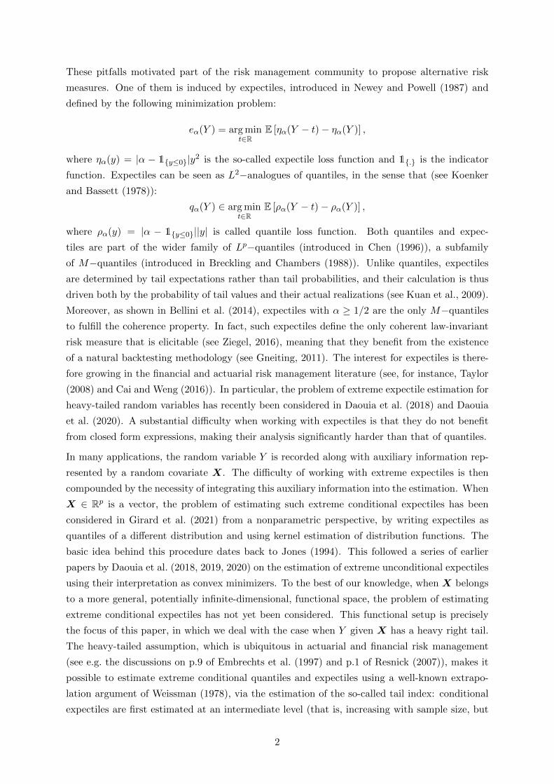
These pitfalls motivated part of the risk management community to propose alternative risk
measures. One of them is induced by expectiles, introduced in Newey and Powell (1987) and
defined by the following minimization problem:
eα(Y ) = arg mint∈R
E [ηα(Y − t)− ηα(Y )] ,
where ηα(y) = |α − 1{y≤0}|y2 is the so-called expectile loss function and 1{.} is the indicator
function. Expectiles can be seen as L2−analogues of quantiles, in the sense that (see Koenker
and Bassett (1978)):
qα(Y ) ∈ arg mint∈R
E [ρα(Y − t)− ρα(Y )] ,
where ρα(y) = |α − 1{y≤0}||y| is called quantile loss function. Both quantiles and expec-
tiles are part of the wider family of Lp−quantiles (introduced in Chen (1996)), a subfamily
of M−quantiles (introduced in Breckling and Chambers (1988)). Unlike quantiles, expectiles
are determined by tail expectations rather than tail probabilities, and their calculation is thus
driven both by the probability of tail values and their actual realizations (see Kuan et al., 2009).
Moreover, as shown in Bellini et al. (2014), expectiles with α ≥ 1/2 are the only M−quantiles
to fulfill the coherence property. In fact, such expectiles define the only coherent law-invariant
risk measure that is elicitable (see Ziegel, 2016), meaning that they benefit from the existence
of a natural backtesting methodology (see Gneiting, 2011). The interest for expectiles is there-
fore growing in the financial and actuarial risk management literature (see, for instance, Taylor
(2008) and Cai and Weng (2016)). In particular, the problem of extreme expectile estimation for
heavy-tailed random variables has recently been considered in Daouia et al. (2018) and Daouia
et al. (2020). A substantial difficulty when working with expectiles is that they do not benefit
from closed form expressions, making their analysis significantly harder than that of quantiles.
In many applications, the random variable Y is recorded along with auxiliary information rep-
resented by a random covariate X. The difficulty of working with extreme expectiles is then
compounded by the necessity of integrating this auxiliary information into the estimation. When
X ∈ Rp is a vector, the problem of estimating such extreme conditional expectiles has been
considered in Girard et al. (2021) from a nonparametric perspective, by writing expectiles as
quantiles of a different distribution and using kernel estimation of distribution functions. The
basic idea behind this procedure dates back to Jones (1994). This followed a series of earlier
papers by Daouia et al. (2018, 2019, 2020) on the estimation of extreme unconditional expectiles
using their interpretation as convex minimizers. To the best of our knowledge, when X belongs
to a more general, potentially infinite-dimensional, functional space, the problem of estimating
extreme conditional expectiles has not yet been considered. This functional setup is precisely
the focus of this paper, in which we deal with the case when Y given X has a heavy right tail.
The heavy-tailed assumption, which is ubiquitous in actuarial and financial risk management
(see e.g. the discussions on p.9 of Embrechts et al. (1997) and p.1 of Resnick (2007)), makes it
possible to estimate extreme conditional quantiles and expectiles using a well-known extrapo-
lation argument of Weissman (1978), via the estimation of the so-called tail index: conditional
expectiles are first estimated at an intermediate level (that is, increasing with sample size, but
2

not too high), and these estimates are then extrapolated using the shape of the conditional
heavy-tailed distribution to obtain estimators of properly extreme conditional expectiles.
Our paper is organized as follows. Section 2 introduces our notation, assumptions, and the
general idea behind our approach, in which we adapt the two-step, extreme conditional quantile
estimation methodology of Gardes and Girard (2012) to the estimation of extreme functional
expectiles. Section 3 gives the asymptotic properties of our estimator of the so-called interme-
diate functional expectiles, which are the basic building blocks of our estimators of properly
extreme functional expectiles considered in Section 4. In the latter section, we will explain that
the estimation of the functional tail index of Y given X is crucial, and in Section 5 we suggest
and study a handful of estimators of this quantity. Section 6 proposes a simulation study to
give an overview of the performance of our procedure. Section 7 concludes by showcasing our
technique on a real financial data example. All proofs are relegated to the Appendix.
2 Notation and assumptions
Let (Xi, Yi), i = 1, . . . , n be independent copies of a random pair (X, Y ) in E×R, where E is a
functional space endowed with a semi-metric d. We assume that the probability distribution of
X is non-atomic, and that the topology of E makes it possible to define the family of conditional
distributions of Y given X = x. For all x ∈ E, the conditional survival function (c.s.f.) of Y
given X = x is denoted by F (y|x) = P (Y > y|X = x). Discussing the existence of regular
versions of F (·|·) is beyond the scope of this paper; it is guaranteed when (E, d) is a Polish
space, see Theorem 1 and its discussion in Chang and Pollard (1997). When d is a semi-metric
defined exclusively on low-frequency components of a truncated basis expansion (for example
when E = L2[0, 1]), the relevant conditional distributions will be defined with respect to the
quotient space of E by the equivalence relation considering that two elements are different if
and only if one pair of their low-frequency components are different. This quotient space is
then essentially a finite-dimensional linear space on which conditional distributions indeed exist,
the price to pay being of course that the conditional distributions only identify lower-frequency
components.
In this context, Gardes and Girard (2012) address the estimation of the conditional quantiles of
Y given X = x, defined by q(α|x) = inf{y ∈ R |F (y|x) ≤ 1− α
}, when the quantile level α is
extreme, i.e. α = αn → 1 as n → ∞. We briefly describe here their two-step approach. First,
the c.s.f. is estimated thanks to a functional kernel estimator, also considered for instance in
Ferraty et al. (2006) and Ferraty et al. (2007):
Fn(y|x) =1
n
n∑i=1
K
(d (x,Xi)
hn
)1{Yi>y}
/µ
(1)K (x, hn) , (2.1)
where (hn) is a positive bandwidth sequence such that hn → 0 as n → ∞, K : [0,∞) → [0,∞)
is a kernel function (namely, positive and measurable), and for all b ≥ 0,
µ(b)K (x, hn) =
1
n
n∑i=1
Kb
(d (x,Xi)
hn
)
3

is the empirical counterpart of the quantity µ(b)K (x, hn) := E
[Kb (d(x,X)/hn)
]. We high-
light that the particular case of the uniform kernel K(t) = 1{0≤t≤1} leads to µ(b)K (x, hn) =
P (X ∈ B(x, hn)) =: π(x, hn), the so-called small ball probability of X, see Ferraty et al. (2007)
for a discussion on this topic. More generally, we assume that
(K)K is a function with support [0, 1] and there exist 0 < c1 < c2 <∞ such that c1 ≤ K(t) ≤ c2
for all t ∈ [0, 1].
One may also suppose without loss of generality that K integrates to one. In this case, K is
called a type I kernel, see Definition 4.1 in Ferraty and Vieu (2006).
Second, the functional estimator of conditional quantiles q(α|x) is defined via the generalized
inverse of (2.1):
qn(α|x) = inf{y ∈ R | Fn(y|x) ≤ 1− α
}. (2.2)
In the situation where α ∈ (0, 1) is fixed, weak and strong consistency are proved respectively in
Stone (1977) and Gannoun (1990) while asymptotic normality is shown in Stute (1986), Samanta
(1989) and Berlinet et al. (2001) when E is finite-dimensional and by Ferraty et al. (2005)
for a general metric space under dependence assumptions. In Gardes and Girard (2012), the
asymptotic distribution of the estimator (2.2) is investigated when estimating extreme quantiles,
i.e. when α = αn → 1 as n→∞.
In this paper, we propose a similar approach for functional expectile regression. For that purpose,
let us recall that, from Jones (1994), the expectile e(α|x) of level α of Y |X = x may be seen as
the quantile of level α associated to the c.s.f. E(y|x) defined by:
E(y|x) =E[(Y − y)1{Y >y} |X = x
]E [|Y − y| |X = x]
.
Introducing, for a nonnegative integer k and provided the expectations exist,
ψ(k)(y|x) = E[(Y − y)k 1{Y >y} |X = x
]and m(k)(y|x) = E
[(Y − y)k |X = x
], (2.3)
it thus follows that e(α|x) = inf{y ∈ R |E(y|x) ≤ 1− α}, with
E(y|x) =ψ(1)(y|x)
2ψ(1)(y|x)−m(1)(y|x). (2.4)
In view of (2.3), we decide to build our estimator upon the following two random quantities:
ψ(k)n (y|x) =
1
n
n∑i=1
(Yi − y)kK
(d (x,Xi)
hn
)1{Yi>y}
/µ
(1)K (x, hn) ,
m(k)n (y|x) =
1
n
n∑i=1
(Yi − y)k K
(d (x,Xi)
hn
)/µ
(1)K (x, hn).
The quantities ψ(k)n (y|x) and m
(k)n (y|x) are (under technical conditions) consistent estimators of
ψ(k)(y|x) and m(k)(y|x), respectively. The c.s.f. E(·|x) defined in (2.4) is then estimated by:
En(y|x) =ψ
(1)n (y|x)
2ψ(1)n (y|x)− m(1)
n (y|x). (2.5)
4

We refer to Girard et al. (2021) for a similar approach in the case where the covariate X is
finite-dimensional.
In the following section and below, our aim is to estimate e(α|x) when the expectile level is
extreme, i.e. α = αn → 1 as n→∞. We introduce several modelling and regularity assumptions
in this respect. We first assume that Y |X = x has a heavy-tailed distribution, namely, there
exists γ(x) > 0 such that the c.s.f. is regularly varying at infinity with index −1/γ(x):
∀y > 0, limt→∞
F (ty|x)
F (t|x)= y−1/γ(x). (2.6)
We refer to Bingham et al. (1989) for a general account on regular variation. In our context,
γ(x) is referred to as the functional tail index since it tunes the tail heaviness of the conditional
distribution of Y given X = x. More precisely, the heavy tail condition (2.6) is refined in the
following way:
C1(γ(x)) There exists γ(x) > 0 such that F (·|x) is continuously differentiable and satisfies
limy→∞
yF′(y|x)
F (y|x)= −1/γ(x).
It follows from Theorem 1.1.11 in de Haan and Ferreira (2006) that condition (2.6) is indeed
satisfied if C1(γ(x)) holds. Another consequence of condition C1(γ(x)) is that the conditional
density function f(·|x) = −F ′(·|x) exists and is also regularly varying, with index −1/γ(x)− 1.
This regularity condition is unlikely to be very restrictive in practice due to the fact that all
commonly used heavy-tailed models satisfy this condition. In addition, Newey and Powell (1987)
point out in their Theorem 1 that continuous differentiability of the c.s.f. is a reasonable sufficient
condition for expectiles to characterize the underlying distribution.
Condition C1(γ(x)) will reveal useful in Section 3 to estimate extreme expectiles e(αn|x) asso-
ciated with intermediate levels αn and located within the sample. For higher levels αn, extreme
expectiles may be located outside the sample. Extrapolation techniques are developed in Sec-
tion 4, and they require a stronger condition on the distribution tail:
C2(γ(x), ρ(x), A(·|x)) There exist γ(x) > 0, ρ(x) ≤ 0 and a positive or negative function A(·|x)
such that:
∀y > 0, limt→∞
1
A(t|x)
(q(1− 1/(ty)|x)
q(1− 1/t|x)− yγ(x)
)=
yγ(x) y
ρ(x) − 1
ρ(x)if ρ(x) < 0,
yγ(x) log y if ρ(x) = 0.
(2.7)
According to Theorem 2.3.9 in de Haan and Ferreira (2006), this so-called second-order condi-
tion (2.7) generalizes condition (2.6), since it is equivalent to
∀y > 0, limt→∞
1
A(1/F (t|x)|x)
(F (ty|x)
F (t|x)− y−1/γ(x)
)= y−1/γ(x) y
ρ(x)/γ(x) − 1
γ(x)ρ(x).
Our last assumption is a local Lipschitz condition on the conditional moments. Similar conditions
are used, for instance, in Krzyzak (1986), or more recently in Daouia et al. (2013) and El Methni
5
et al. (2014) in the context of conditional extreme value analysis with a finite-dimensional
covariate. Let us denote by B(x, r) the ball with center x ∈ E and radius r > 0, associated
with the semi-metric d, and by ∨ the maximum operator.
(L) One has m(2)(0|x) = E[Y 2 |X = x
]<∞ and there exist c, r > 0 such that
∀x′ ∈ B(x, r),∣∣∣m(1)(0|x′)−m(1)(0|x)
∣∣∣ ∨ ∣∣∣m(2)(0|x′)−m(2)(0|x)∣∣∣ ≤ c d (x,x′) .
We conclude this paragraph by introducing some notation, which will prove very useful, for the
oscillation of the c.s.f. F (·|x) above a high level yn:
ωhn(yn|x) = supz≥yn
x′∈B(x,hn)
1
log z
∣∣∣∣logF (z|x′)F (z|x)
∣∣∣∣ .The quantity ωhn(yn|x) measures the discrepancy between the extremes of the conditional dis-
tributions of Y at neighboring points. Similar quantities are introduced in Gardes and Stupfler
(2014, 2019) and Stupfler (2013, 2016). In order to get an idea of the typical asymptotic behavior
of ωhn(yn|x), consider the Karamata representation of F (·|x):
∀z ≥ 1, F (z|x) = z−1/γ(x) exp
(η(z|x) +
∫ z
1
ε(u|x)
udu
),
where η(·|x) and ε(·|x) are measurable functions converging, respectively, to a constant and 0
at infinity, see Theorem 1.3.1 in Bingham et al. (1989). In this context, it is straightforward to
prove that if there are c, r > 0 and z0 > 1 with
∀x′ ∈ B(x, r),∣∣γ(x)− γ(x′)
∣∣ ∨ supz≥z0
∣∣∣∣η(z|x)− η(z|x′)log z
∣∣∣∣ ∨ supz≥1
∣∣ε(z|x)− ε(z|x′)∣∣ ≤ c d (x,x′) ,
(2.8)
then ωhn(yn|x) = O(hn).
3 Intermediate functional expectile estimation
We consider from now on the case when γ(x) < 1 and Y− := max(−Y, 0) has a finite first
conditional moment. These conditions combined ensure that E(|Y | |X = x) <∞ and thus that
conditional expectiles at any order exist indeed. These will be our minimal working conditions
throughout this paper.
Let us consider a sequence (αn) such that αn → 1 as n→∞. It has been established in Gardes
and Girard (2012, Theorem 2) that the functional estimator (2.2) of the extreme quantile q(αn|x)
is asymptotically Gaussian provided that n(1− αn)π(x, hn)→∞ as n→∞. In this situation,
q(α|x) is referred to as an intermediate conditional quantile. It is, for n large enough, located
within the sample since there is then almost surely at least one sample point in the region
B(x, h) × (q(α|x),∞) ⊂ E × R, see Gardes and Girard (2012, Lemma 4). Condition n(1 −αn)π(x, hn) → ∞ in fact ensures that there will be a growing number of observations larger
than the conditional quantile to be estimated. In this section, we propose a similar approach
for estimating intermediate conditional expectiles. Let
en(αn|x) = inf{y ∈ R | En(y|x) ≤ 1− αn
}. (3.1)
6

Here En(y|x) is defined in Equation (2.5). We start by studying the joint asymptotic distri-
bution of estimators (2.2) and (3.1), as this will be crucial in our construction of extrapolation
procedures in Section 5. To this end, let us introduce
σ−1n (x) =
(n(1− αn)
µ(1)K (x, hn)2
µ(2)K (x, hn)
)1/2
.
Note that, under (K), σ−1n (x) and
√n(1− αn)π(x, hn) are of the same asymptotic order since
(c1/c2)2π(x, hn) ≤µ
(1)K (x, hn)2
µ(2)K (x, hn)
≤ (c2/c1)2π(x, hn).
The following result may be seen as a functional version of Theorem 1 in Girard et al. (2021).
It establishes the joint asymptotic normality of J empirical conditional intermediate expectiles
en(αn,j |x) with 1 − αn,j = τj(1 − αn), 0 < τ1 < · · · < τJ ≤ 1, together with an empirical
conditional intermediate quantile qn(an|x).
Theorem 1. Assume that (K), (L) and C1(γ(x)) hold with γ(x) < 1/2. Suppose that there
exists δ ∈ (0, 1) such that E[Y 2+δ− |X = x] < ∞. Let αn → 1, hn → 0 as n → ∞ and τ > 0,
0 < τ1 < τ2 < · · · < τJ ≤ 1 with
1− an = τ(1− αn)(1 + o(1)) and 1− αn,j = τj(1− αn),
for j ∈ {1, . . . , J}. Assume further that n(1− αn)π(x, hn)→∞ and
σ−1n (x) log(1− αn)ωhn ((1− δ)(e(αn|x) ∧ q(an|x))|x)→ 0. (3.2)
Then,
σ−1n (x)
{(en(αn,j |x)
e(αn,j |x)− 1
)1≤j≤J
,
(qn(an|x)
q(an|x)− 1
)}d−→ N
(0J+1, γ
2(x)Σ(x)),
where Σ(x) is the symmetric matrix having entries
Σj,l(x) = τ−1l
[1
1− 2γ(x)
(τjτl
)−γ(x)
− 1
],
Σj,J+1(x) = τ−1j
(τjτ
)γ(x)[(
1
γ(x)−1 − 1∧ τjτ
)1−γ(x)
+
(1
γ(x)−1 − 1∧ τjτ
)−γ(x)
−(τjτ
)−γ(x)],
ΣJ+1,J+1(x) = τ−1,
for (j, l) ∈ {1, . . . , J}2 with j ≤ l.
In particular, Theorem 1 provides the following asymptotic normality result for en(αn|x), which
may be seen as a functional version of Theorem 2 in Daouia et al. (2018):
σ−1n (x)
(en(αn|x)
e(αn|x)− 1
)d−→ N
(0,
2γ3(x)
1− 2γ(x)
).
7

This is done under the assumptions γ(x) < 1/2 and E[Y 2+δ− |X = x] < ∞. These essentially
guarantee that |Y | has a finite conditional moment of order 2+δ, a reasonable assumption in this
context of estimating conditional expectiles which generalize the conditional mean. In addition,
condition (3.2) ensures that the bias incurred by the use of the functional kernel smoothing
technique in this conditional extreme value setting is asymptotically negligible.
As we have already noted, Theorem 1 requires the condition n(1 − αn)π(x, hn) → ∞ which
prevents the estimation of expectiles at arbitrarily large levels αn. In the next section, we
propose to overcome this issue using an extrapolation tool.
4 Extreme functional expectile extrapolation
Our aim in this section is to estimate conditional expectiles at an extreme level βn such that
n(1−βn)π(x, hn)→ c <∞. In extreme quantile estimation, a well-known approach is to use the
Weissman extrapolation device, see Theorem 4.3.8 in de Haan and Ferreira (2006): remarking
that under C1(γ(x)),
q(βn|x) =
(1− αn1− βn
)γ(x)
q(αn|x)(1 + o(1)), (4.1)
the extreme conditional quantile q(βn|x) can therefore be estimated using the intermediate
empirical quantile qn(αn|x) and a suitable estimator of γ(x). We refer for instance to Daouia
et al. (2011) or Gardes and Girard (2012) for extreme conditional quantile estimators developed
on this basis. In the expectile case, a similar approach can be adopted based on the convergence
limα→1
F (e(α|x)|x)
1− α= γ(x)−1 − 1. (4.2)
This is a consequence of the heavy-tailed assumption (2.6): see Bellini et al. (2014, Theorem 11)
and more recently Daouia et al. (2018, Proposition 1). This convergence is in fact equivalent to
limα→1
e(α|x)
q(α|x)=(γ(x)−1 − 1
)−γ(x), (4.3)
meaning that extreme quantiles and extreme expectiles are asymptotically proportional. As a
consequence, Equation (4.1) also holds for expectiles. As proposed in Girard et al. (2021) in
the finite-dimensional context, we introduce a Weissman-type estimator of functional extreme
expectiles:
eWn,αn(βn|x) =
(1− αn1− βn
)γαn (x)
en(αn|x), (4.4)
where γαn(x) is any estimator of γ(x). Using the second order assumption C2(γ(x), ρ(x), A(·|x)),
we can state the asymptotic behavior of eWn,αn(βn|x) under high-level conditions.
Theorem 2. Assume that (K), (L) and C2(γ(x), ρ(x), A(·|x)) hold with γ(x) < 1/2 and ρ(x) <
0. Suppose that there exists δ ∈ (0, 1) such that E[Y 2+δ− |X = x] < ∞. Let αn → 1, βn → 1
and hn → 0 be such that n(1 − αn)π(x, hn) → ∞ and n(1 − βn)π(x, hn) → c < ∞ as n → ∞.
Assume further that
i) σ−1n (x) log(1− αn)ωhn ((1− δ)e(αn|x)|x)→ 0,
8

ii) σ−1n (x)/ log ((1− αn)/(1− βn))→∞,
iii) σ−1n (x)A
((1− αn)−1|x
)→ λ1 ∈ R and σ−1
n (x)/q(αn|x)→ λ2 ∈ R.
If, in addition, σ−1n (x) (γαn(x)− γ(x))
d−→ Γ, where Γ is a nondegenerate distribution, then
σ−1n (x)
log ((1− αn)/(1− βn))
(eWn,αn(βn|x)
e(βn|x)− 1
)d−→ Γ.
The Weissman-type estimator eWn,αn(βn|x) is built on the previous estimator en(αn|x) of the
intermediate expectile, hence the conditions γ(x) < 1/2 and E[Y 2+δ− |X = x] < ∞ to ensure
the asymptotic normality of en(αn|x). In order to relax these assumptions, one may exploit the
asymptotic proportionality relationship (4.3) to define another Weissman-type estimator:
eWn,αn(βn|x) =
(1− αn1− βn
)γ(x)
qn(αn|x)(γ(x)−1 − 1
)−γ(x). (4.5)
The following high-level result establishes the asymptotic properties of this estimator, under
weaker conditions than those of Theorem 2.
Theorem 3. Assume that (K) and C2(γ(x), ρ(x), A(·|x)) hold with γ(x) < 1 and ρ(x) < 0.
Suppose that E [Y−|X = x] < ∞. Let αn → 1, βn → 1 and hn → 0 be such that n(1 −αn)π(x, hn)→∞ and n(1− βn)π(x, hn)→ c <∞ as n→∞. Assume further that
i) σ−1n (x) log(1− αn)ωhn ((1− δ)q(αn|x)|x)→ 0 for some δ > 0,
ii) σ−1n (x)/ log ((1− αn)/(1− βn))→∞,
iii) σ−1n (x)A
((1− αn)−1|x
)→ λ1 ∈ R and σ−1
n (x)/q(αn|x)→ λ2 ∈ R.
If, in addition, σ−1n (x) (γαn(x)− γ(x))
d−→ Γ, where Γ is a nondegenerate distribution, then,
σ−1n (x)
log ((1− αn)/(1− βn))
(eWn,αn(βn|x)
e(βn|x)− 1
)d−→ Γ.
To illustrate these results, let us consider the case 1 − αn = (nπ(x, hn))−a and 1 − βn =
(nπ(x, hn))−b with 0 < a < 1 < b and c = 0. In this case the two conditions n(1−αn)π(x, hn)→∞ and n(1− βn)π(x, hn)→ c = 0 turn into the single condition nπ(x, hn)→∞. We shall also
work under Assumption (2.8) which entails ωhn(yn|x) = O(hn) when yn → ∞. Recalling that
the rate of convergence σ−1n (x) grows like
√n(1− αn)π(x, hn) = (nπ(x, hn))(1−a)/2, we find that
the other conditions on αn, βn and hn required in Theorem 2 and Theorem 3 can be simplified
as (nπ(x, hn))(1−a)/2 log(nπ(x, hn))hn → 0, as n→∞, and a > 1/(1 + 2ξ) with ξ = min(γ,−ρ).
We illustrate the implications of this discussion on two classical examples for X.
9

Example 1. If X is a fractal process of order τ > 0 with respect to the semi-metric d, then
π(x, hn) ∼ Chτn, as hn → 0, for some C > 0, see Definition 13.1 in Ferraty and Vieu (2006). This
situation includes the finite p−dimensional case, where τ = p. Here, the conditions nπ(x, hn)→∞ and (nπ(x, hn))(1−a)/2 log(nπ(x, hn))hn → 0 imply that one can choose hn = n−θ with
θ ∈(
1− a2 + τ(1− a)
,1
τ
).
Let us stress that there is no constraint on b, apart from b > 1, and therefore extreme functional
expectiles of level converging to 1 at an arbitrarily fast polynomial rate nb(τθ−1), b > 1, can
then be estimated with (4.4) or (4.5). Letting a ↓ 1/(1 + 2ξ), the bias associated with the
smoothing (condition i) in Theorem 2 and Theorem 3) and the bias associated with the tail
approximations (condition iii) in Theorem 2 and Theorem 3) are of the same order. It is
then possible to balance the squared bias and the variance of the Weissman type estimators by
choosing θ = ξ/(1 + (2 + τ)ξ). This yields a polynomial rate of convergence n−ξ/(1+(2+τ)ξ).
Example 2. If X is an exponential-type process with orders τ1, τ2 ≥ 0 with respect to the
semi-metric d, then π(x, hn) ∼ C exp(−h−τ1n (− log hn)τ2), as hn → 0, for some C > 0, see
Definition 13.4 in Ferraty and Vieu (2006). We refer to Li and Shao (2001) for several examples
of Gaussian processes which are exponential-type processes for the metric associated with the
supremum norm in functional spaces. Here, we focus on the case τ2 = 0 for the sake of simplicity,
and we let hn = (log n− κ log log n)−1/τ1 with
κ ∈(
0,2
τ1(1− a)
).
This choice yields 1−βn ∼ C−b(log n)−bκ. The considered Weissman type estimators are, in this
case, limited to the estimation of extreme functional expectiles of (arbitrary) logarithmic level.
Finally, balancing the bias and variance by letting κ ↑ 2/[τ1(1− a)] yields a logarithmic rate of
convergence (log n)−1/τ1 . This slow rate of convergence is a consequence of the exponentially
fast decay of the small ball probability π(x, hn) as hn → 0. One way to avoid this vexing effect
is to consider projection-type semi-metrics, for instance using functional Principal Component
Analysis; this will be tried out in our finite-sample illustrations.
In view of Theorem 2 and Theorem 3, the asymptotic distribution of the Weissman-type
estimators of eWn,αn(βn|x) and eWn,αn(βn|x) is exactly determined by that of the functional tail
index estimator γαn(x) used in its construction. It is therefore essential to provide estimators of
γ(x) having good performance. The next section is devoted to this problem from an expectile
perspective.
5 Functional tail index estimation
The estimation of the tail index is a central problem in the extreme-value literature. In the
unconditional heavy-tailed setting, the most popular estimator is arguably that of Hill (1975),
and is based on the mean of the log-excesses. This idea of averaging log-excesses was adapted
10
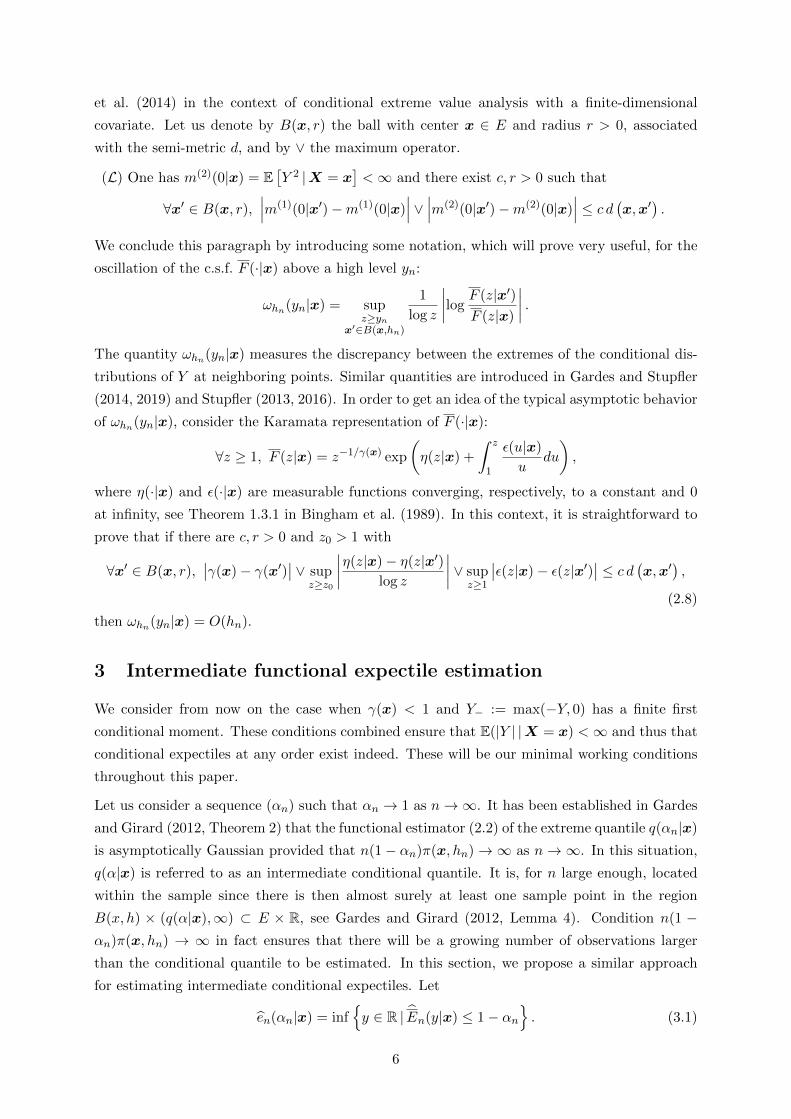
to the conditional framework in Gardes and Girard (2012): for a given integer J ≥ 2,
γ(J)αn (x) =
1
log(J !)
J∑j=1
log
(qn (1− (1− αn)/j|x)
qn (αn|x)
). (5.1)
The asymptotic properties of γ(J)αn (x) may be found in Theorem 4 and Corollary 1 of Gardes and
Girard (2012) under mild conditions. Our first contribution here is to strengthen their results
by making the bias term explicit; this will inform the construction of another of our estimators
below. In the Appendix, we provide the joint asymptotic distribution of γ(J)αn (x) and estimators
of extreme conditional quantiles (see Theorem 7).
Theorem 4. Assume that (K) and C2(γ(x), ρ(x), A(·|x)) hold. Let αn → 1, hn → 0 be such
that n(1− αn)π(x, hn)→∞ and
i) σ−1n (x) log(1− αn)ωhn ((1− δ)q(αn|x)|x)→ 0, for some δ > 0,
ii) σ−1n (x)A
((1− αn)−1|x
)→ λ1 ∈ R.
Then,
σ−1n (x)
(γ(J)αn (x)− γ(x)
)d−→ N
1
log(J !)
J∑j=1
jρ(x) − 1
ρ(x)
λ1,J(J − 1)(2J − 1)
6 log(J !)2γ2(x)
.
As pointed out in Daouia et al. (2011), the choice J = 9 leads to the smallest asymptotic
variance: in this case the factor J(J − 1)(2J − 1)/(6 log(J !)2) is approximately equal to 1.245.
Second, to define an estimator of the functional tail index γ(x) solely based on the use of
expectiles, we introduce an alternative device based on the asymptotic relationship (4.2): this
relationship implies
γ(x) = limα→1
1− α1− α+ F (e(α|x)|x)
.
This leads us to consider the following estimator:
γαn(x) =1− αn
1− αn + Fn(en(αn|x)|x). (5.2)
Note that this expectile-based estimator was first introduced in Girard et al. (2021) in the finite-
dimensional covariate setting. The next result gives the asymptotic distribution of the functional
tail index estimator γαn(x).
Theorem 5. Assume that (K), (L) and C2(γ(x), ρ(x), A(·|x)) hold with γ(x) < 1/2. Suppose
that there exists δ ∈ (0, 1) such that E[Y 2+δ− |X = x] < ∞. Let αn → 1 and hn → 0 such that
n(1− αn)π(x, hn)→∞ as n→∞ and
i) σ−1n (x) log(1− αn)ωhn ((1− δ)e(αn|x)|x)→ 0,
ii) σ−1n (x)A
((1− αn)−1|x
)→ λ1 ∈ R and σ−1
n (x)/q(αn|x)→ λ2 ∈ R.
11

Then, σ−1n (x) (γαn(x)− γ(x)) is asymptotically Gaussian with mean
b(x) =γ(x)
(γ(x)−1 − 1
)1−ρ(x)
1− γ(x)− ρ(x)λ1 + γ2(x)
(γ(x)−1 − 1
)γ(x)+1 E[Y |X = x]λ2
and variance
V (x) =γ3(x)(1− γ(x))
1− 2γ(x).
The main advantage of γαn(x) compared to γ(J)αn (x) is its much smaller asymptotic variance
for small values of γ(x). However, the asymptotic normality of γαn(x) requires the condition
γ(x) < 1/2, and the variance explodes when γ(x) is close to 1/2. To avoid this drawback, we
propose to replace the “direct” estimator of the functional expectile en(αn|x) in Equation (5.2)
by an “indirect” estimator designed from Equation (4.3). We thus propose a third estimator
combining the two previous approaches, having a lower asymptotic variance compared to γ(J)αn (x),
and asymptotically Gaussian under weaker assumptions compared to γαn(x):
γ(J)αn (x) =
1− αn
1− αn + Fn
((γ
(J)αn (x)−1 − 1
)−γ(J)αn (x)qn(αn|x)|x
) . (5.3)
The following result provides the asymptotic normality of this new estimator.
Theorem 6. Assume that (K) and C2(γ(x), ρ(x), A(·|x)) hold with γ(x) < 1. Let αn → 1,
hn → 0 be such that n(1− αn)π(x, hn)→∞ as n→∞ and
i) σ−1n (x) log(1− αn)ωhn ((1− δ)q(αn|x) ∧ e(αn|x)|x)→ 0, for some δ > 0,
ii) σ−1n (x)A
((1− αn)−1|x
)→ λ1 ∈ R and σ−1
n (x)/q(αn|x)→ λ2 ∈ R.
Then, σ−1n (x)
(γ
(J)αn (x)− γ(x)
)is asymptotically Gaussian with mean
bJ(x) =
h(γ(x))1
log(J !)
J∑j=1
jρ(x) − 1
ρ(x)
− (1− γ(x))
(γ(x)−1 − 1
)−ρ(x) − 1
ρ(x)
λ1
and variance VJ(x) = γ2(x)vJ(x), with
vJ(x) = h (γ(x))2 J(J − 1)(2J − 1)
6 log(J !)2− 2
(1− γ(x))2
(γ(x)−1 − 1) ∨ 1+ (1− γ(x))
− (1− γ(x))h(γ(x))2j∗((γ(x)−1 − 1) ∧ 1
)−1+ (J − j∗)(J − j∗ + 1)− 2J
log(J !),
where h(t) = 1− (1− t) log(t−1 − 1
)and j∗ ∈ {0, . . . , J} is such that τj∗ < γ(x)−1 − 1 ≤ τj∗+1,
in which we set τ0 = 0, τj = (J − j + 1)−1 for all j ∈ {1, . . . , J}, and τJ+1 =∞.
We can notice that the variance term vJ(x) = VJ(x)/γ2(x) may also be written:
vJ(x) = h (γ(x))2 J(J − 1)(2J − 1)
6 log(J !)2+ (1− γ(x))2
(1
1− γ(x)− 2
(γ(x)−1 − 1) ∨ 1
)− 2
(1− γ(x))h (γ(x))
log(J !)
J−1∑j=1
[(τj ∨ (γ(x)−1 − 1)
)−1 −(1 ∨ (γ(x)−1 − 1)
)−1].
12

In the Appendix, the proof of Theorem 6 is provided using the above formula. Straightforward
calculations lead to the equivalence of these two expressions.
It appears that this new estimator is asymptotically Gaussian under weaker conditions than those
imposed on γαn(x) and has only one source of bias (in the sense that its bias does not depend
on λ2, coming from the condition σ−1n (x)/q(αn|x) → λ2 ∈ R). We investigate the asymptotic
variances of the three estimators γ(9)αn (x), γ
(9)αn (x) and γαn(x) in Figure 1. We can see here
that γαn(x) seems to have the lowest variance among all three estimators for γ(x) ∈ [0, 0.25].
The new estimator γ(9)αn (x) seems to strike a middle ground, in the sense that it appears to
have the lowest variance when the conditional tail index lies between approximately 0.25 and
0.5. In addition, its variance remains relatively stable when γ(x) ∈ [0.5, 1], even though the
quantile-based estimator γ(9)αn (x) has the lowest variance in this interval.
Finally, let us note that Theorem 1 opens the door to the design of estimators of the functional
tail index based on a combination of several empirical conditional intermediate expectiles. One
could for instance consider a Pickands-type estimator (Pickands, 1975) based on the following
three empirical conditional intermediate expectiles: en(1 − kn/n|x), en(1 − kn/(2n)|x) and
en(1 − kn/(4n)|x) with kn = n(1 − αn), which corresponds to considering three intermediate
expectile estimators as in Theorem 1 with τ1 = 1/4, τ2 = 1/2 and τ3 = 1.
0.0 0.2 0.4 0.6 0.8 1.0
0.0
0.2
0.4
0.6
0.8
1.0
1.2
Asymptotic variances
gamma
v
Figure 1: Asymptotic variances of γ(9)αn (x) (black curve), γ
(9)αn (x) (red curve) and γαn(x) (blue
curve) as functions of γ(x) ∈ [0, 1].
13

6 Illustration on simulated data
We briefly illustrate here the finite-sample performance of the estimators on N = 500 replications
of an independent sample of size n = 500 (resp. 2,000) from a random pair (X, Y ), where
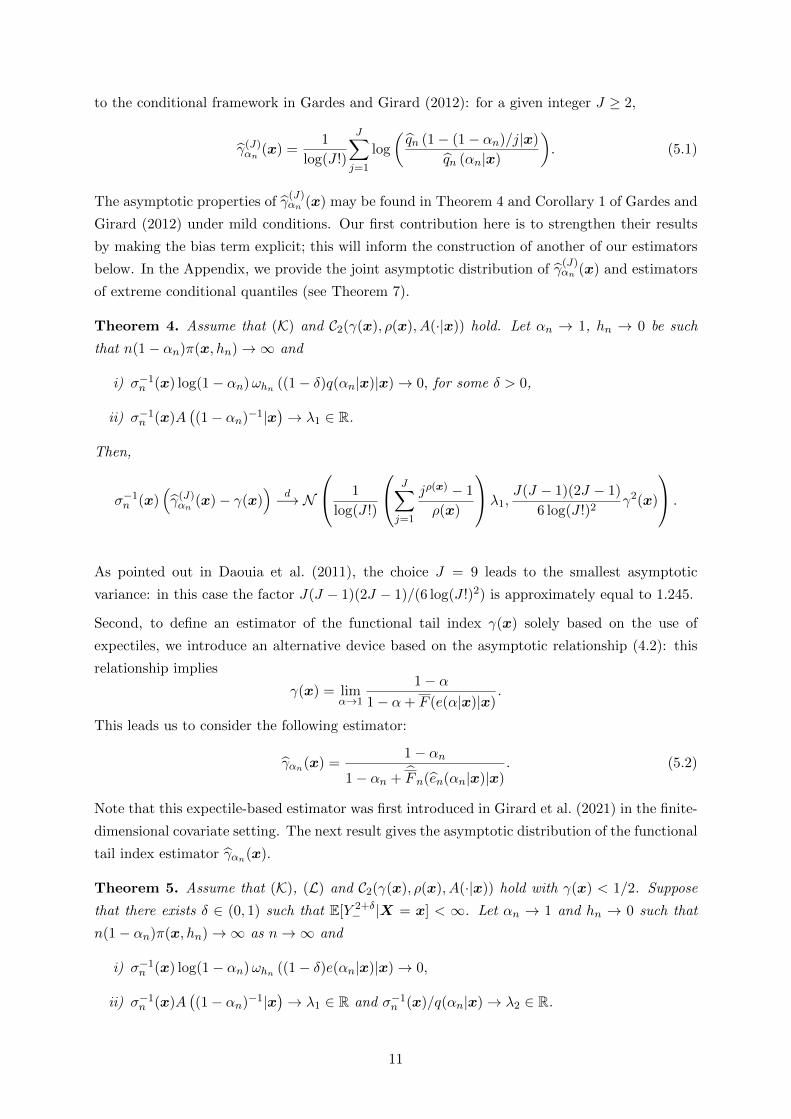
X ∈ E = L2[0, 1]. Here, X may be three different stochastic processes:
• (X1): A process given by Xt = cos(2πZt) for all t ∈ [0, 1] with Z a latent uniform random
variable on [1/4, 1], and the functional tail index is given by γ(X) =(8||X||22 − 3
)/2.5
with ||X||22 =∫ 1
0 X2t dt = 1
2
(1 + sin(4πZ)
4πZ
). A similar specification is used in Gardes and
Girard (2012); in this context γ(X) ∈ [0.06, 0.61] and d is the standard metric on L2[0, 1].
• (X2): A process given for all t ∈ [0, 1] by
Xt =√
250∑j=1
(−1)j+1
jZj cos(jπt),
where the Zj are i.i.d. uniform on [−1, 1]. Such an example is considered in Kato (2012).
In this more difficult example, it is suitable to consider a (functional) Principal Com-
ponent Analysis semi-metric (see Chapter 3 in Ferraty and Vieu (2006) and particularly
Section 3.4), defined as
dq,PCA(X,X ′) =
√√√√ q∑k=1
{∫ 1
0(Xt −X ′t)ϕk(t)dt
}2
,
where ϕ1, . . . , ϕq are eigenfunctions of the unobserved covariance operator (s, t) 7→ E(XsXt)
associated with its first q eigenvalues λ1 ≥ λ2 ≥ · · · ≥ λq. This semi-metric induces a semi-
norm by setting ||X||q,PCA = dq,PCA(X,0) where 0 is the zero function. A numerical study
using the R package fdapace (see Carroll et al. (2021)) shows that a choice of q = 2 leads
to an explained variance around 80%. We thus take q = 2, estimate ϕ1 and ϕ2 with the R
function FPCA in this package, and consider a conditional tail index γ(X) = 0.25+2||X||2.
• (X3): A standard Brownian bridge (Xt) on [0, 1]. Inspired by the previous model, we keep
γ(X) = 0.25 + 2||X||2. Here also, around 80% of the variance is typically explained with
the first two eigenfunctions and we take q = 2 in this example too.
An overview of the shape of the three covariates considered is proposed in Figure 2 through
the simulation of a few realizations. The first kind of process may be found in areas like
environmental sciences (representing sound or light waves). The other two are more frequent in
finance (see Metwally and Atiya (2002) for an example). Given X, the random variable Y has,
in all cases, a Pareto distribution with c.s.f. F (y|X) = y−1/γ(X), y > 1.
The aim of this study is to assess the quality of the estimates of the extreme functional expectile
e(βn|x) with βn = 0.995 (1 − 2.5/n when n = 500 and 1 − 10/n when n = 2,000). For that
purpose, the Weissman-type estimators (4.4) and (4.5) are used with the kernel K(t) = (1.9 −1.8 t)1{0≤t≤1}. The tail index is estimated with γ
(9)αn (x) and γ
(9)αn (x) defined in (5.1) and (5.3)
14
0.0 0.2 0.4 0.6 0.8 1.0
−1.
0−
0.5
0.0
0.5
1.0
0.0 0.2 0.4 0.6 0.8 1.0
−3
−2
−1
01
2
0.0 0.2 0.4 0.6 0.8 1.0
−0.
50.
00.
51.
0
Figure 2: 10 realizations of the covariate X for models (X1) (left), (X2) (middle) and (X3)
(right).
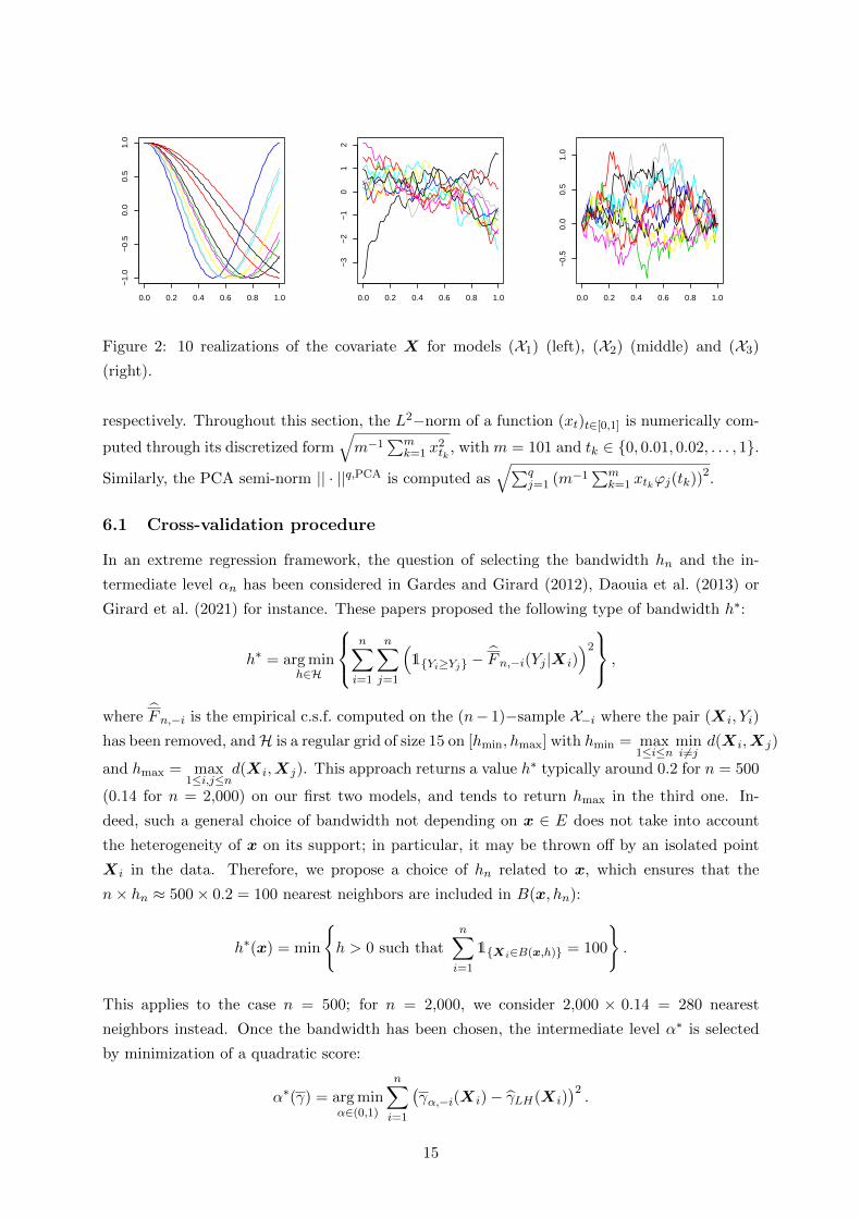
respectively. Throughout this section, the L2−norm of a function (xt)t∈[0,1] is numerically com-
puted through its discretized form√m−1
∑mk=1 x
2tk
, with m = 101 and tk ∈ {0, 0.01, 0.02, . . . , 1}.
Similarly, the PCA semi-norm || · ||q,PCA is computed as√∑q
j=1 (m−1∑m
k=1 xtkϕj(tk))2.
6.1 Cross-validation procedure
In an extreme regression framework, the question of selecting the bandwidth hn and the in-
termediate level αn has been considered in Gardes and Girard (2012), Daouia et al. (2013) or
Girard et al. (2021) for instance. These papers proposed the following type of bandwidth h∗:
h∗ = arg minh∈H
n∑i=1
n∑j=1
(1{Yi≥Yj} − Fn,−i(Yj |Xi)
)2
,
where Fn,−i is the empirical c.s.f. computed on the (n− 1)−sample X−i where the pair (Xi, Yi)
has been removed, andH is a regular grid of size 15 on [hmin, hmax] with hmin = max1≤i≤n
mini 6=j
d(Xi,Xj)
and hmax = max1≤i,j≤n
d(Xi,Xj). This approach returns a value h∗ typically around 0.2 for n = 500
(0.14 for n = 2,000) on our first two models, and tends to return hmax in the third one. In-
deed, such a general choice of bandwidth not depending on x ∈ E does not take into account
the heterogeneity of x on its support; in particular, it may be thrown off by an isolated point
Xi in the data. Therefore, we propose a choice of hn related to x, which ensures that the
n× hn ≈ 500× 0.2 = 100 nearest neighbors are included in B(x, hn):
h∗(x) = min
{h > 0 such that
n∑i=1
1{Xi∈B(x,h)} = 100
}.
This applies to the case n = 500; for n = 2,000, we consider 2,000 × 0.14 = 280 nearest
neighbors instead. Once the bandwidth has been chosen, the intermediate level α∗ is selected
by minimization of a quadratic score:
α∗(γ) = arg minα∈(0,1)
n∑i=1
(γα,−i(Xi)− γLH(Xi)
)2.
15

Here, γα,−i denotes either γ(9)α or γ
(9)α computed on the (n − 1)−sample X−i, and γLH(Xi) is
the local Hill estimator computed on the subset of 100 values {Y (i)j , j = 1, . . . , 100} := {Yj : 0 <
d(Xi,Xj) ≤ h∗(x), j = 1, . . . , n} whose covariate values are within distance h∗(x) of Xi. This
estimator is defined by
γLH(Xi) =1
ki
ki∑j=1
log
Y (i)100−j+1,100
Y(i)
100−ki,100
,
where we set ki = 20 (50 for n = 2,000) and Y(i)
1,100 ≤ . . . ≤ Y(i)
100,100 are the order statistics
associated with {Y (i)j , j = 1, . . . , 100}, sorted in increasing order. This procedure yields selected
values α∗(γ(9)) ' α∗(γ(9)) typically around 0.84 (0.805 for n = 2,000) for (X1), 0.80 (0.815 for
n = 2,000) for (X2) and 0.70 (0.88 for n = 2,000) for (X3).
6.2 Results
In example (X1), Figure 3 displays the performance of the conditional tail index and conditional
expectile estimators on boxplots, within the space of functions {xt 7→ cos(2πzt), t ∈ [0, 1]},depending on the latent variable z ∈ [1/4, 1]. In other words, at each z within a fine grid
of points in [1/4, 1], we estimate the conditional tail index and extreme conditional expectile
estimators given x = (t 7→ cos(2πzt)). The numerical results associated with γ(9)α∗ (x) and γ
(9)α∗ (x)
are in line with the theoretical results illustrated in Figure 1: it appears indeed from the length
of the represented boxplots that the estimator γ(9)α∗ (x) tends to have a lower variance for lower
values of γ(x), and to be slightly more accurate on average, than the estimator γ(9)α∗ (x). Finally,
it seems that both Weissman-type estimators eWn,α∗(βn|x) and eWn,α∗(βn|x) generally perform
similarly at the level 0.995, with an advantage for the direct estimator eWn,α∗(βn|x) in areas
where the tail is heavy, and, by contrast, an advantage for the indirect estimator eWn,α∗(βn|x) in
areas where the tail is light.
In examples (X2) and (X3), contrary to the first example, we can no longer represent the results
as a function of a single univariate latent variable. To visualize our results, we thus propose
to simulate a test sample x1, . . . ,x100 of size 100 (fixed across all samples), and estimate the
extreme expectiles e(βn|x1), . . . , e(βn|x100). The results are reported in Figure 4 as functions of
the L2−norms of xi, 1 ≤ i ≤ 100. In the area where most of the data are typically concentrated,
the proposed estimators provide a good approximation of the conditional tail index and the
conditional extreme expectile. However, in the areas where this is not the case (for unusually
small or large L2−norms), trusting our estimators is of course more difficult. This problem is a
classical problem in the nonparametric literature. Note that the empirical curves are smoothed
with the R function loess, and a smoothing parameter of 0.25. Note also that we computed
the bias-reduced versions of our extreme expectile estimators introduced in Girard et al. (2021)
(dashed lines) which improve the accuracy of the results:eW,BRn,αn (βn|x) = eWn,αn(βn|x)
(1− mn(x)γ(x)
en(αn|x)
)+ mn(x)γ(x),
eW,BRn,αn (βn|x) = eWn,αn(βn|x) + mn(x)γ(x).
(6.1)
16

0.25 0.34 0.43 0.52 0.61 0.7 0.79 0.88 0.97
0.0
0.2
0.4
0.6
0.8
1.0
0.25 0.34 0.43 0.52 0.61 0.7 0.79 0.88 0.97
0.0
0.2
0.4
0.6
0.8
1.0
0.25 0.34 0.43 0.52 0.61 0.7 0.79 0.88 0.97
020
4060
0.25 0.34 0.43 0.52 0.61 0.7 0.79 0.88 0.97
020
4060
Figure 3: Simulation results on a conditional Pareto distribution with model (X1). Top panel:
tail index estimators γ(9)α∗ (·) (green box plots) and γ
(9)α∗ (·) (blue box plots), where at each z ∈
[1/4, 1] we represent estimated values at x = (t 7→ cos(2πzt)), for n = 500 (left) and n = 2,000
(right). The red curve is the true value of γ(·). Bottom panel: Indirect (green box plots) and
direct (blue box plots) expectile estimators eWn,α∗(βn|·) and eWn,α∗(βn|·) based on the tail index
estimator γ(9)α∗ (·) for n = 500 (left) and n = 2,000 (right). The red curve is the true value of
e(βn|·), with βn = 0.995.
These bias-reduced versions have the same asymptotic behavior as the original eWn,αn(βn|x) and
eWn,αn(βn|x) but perform better in finite samples, as illustrated in Figure 4.
7 Real data example
We consider data on the price of the Bitcoin cryptocurrency between January 1, 2012 and
January 8, 2018 on the exchange platform Bitstamp1. We use our estimators to, based on
hourly log-returns of the price of Bitcoin on a given day, estimate the level of extreme swings
of the price of Bitcoin the next day. More specifically, our goal is to estimate extreme expectile
levels of the maximum hourly log-return Y of Bitcoin price based on the information on past
1This dataset is available at https://github.com/FutureSharks/financial-data/tree/master/
pyfinancialdata/data/cryptocurrencies/bitstamp/BTC_USD and is on file with the authors.
17

0.04 0.06 0.08 0.10 0.12
05
1015
2025
Tail index estimators
L2−norm
0.30
0.35
0.40
0.45
0.50
0.04 0.06 0.08 0.10 0.12
05
1015
2025
Expectile estimators
L2−norm
46
810
1214
0.04 0.06 0.08 0.10 0.12
05
1015
2025
Tail index estimators
L2−norm
0.30
0.35
0.40
0.45
0.50
0.04 0.06 0.08 0.10 0.12
05
1015
2025
Expectile estimators
L2−norm
46
810
1214
0.02 0.04 0.06 0.08
05
1020
30
Tail index estimators
L2−norm
0.25
0.30
0.35
0.40
0.45
0.02 0.04 0.06 0.08
05
1020
30
Expectile estimators
L2−norm
34
56
78
910
0.02 0.04 0.06 0.08
05
1020
30
Tail index estimators
L2−norm
0.25
0.30
0.35
0.40
0.45
0.02 0.04 0.06 0.08
05
1020
30
Expectile estimators
L2−norm
34
56
78
910
Figure 4: Histograms of the PCA-norm of the test sample x1, . . . ,x100 of (X2) (first two rows)
and Brownian bridges (X3) (last two rows), and the associated theoretical values of γ(xi) and
e(βn|xi) (red curves) as functions of ||xi||2. On the tail index panels, the median values of
estimates γ(9)α∗ (·) and γ
(9)α∗ (·) are respectively represented with the green and blue curves. On
the expectile panels, the median values of the direct and indirect estimators eWn,α∗(βn|·) and
eWn,α∗(βn|·) (both computed with γ(9)α∗ (·)) are respectively represented with the green and blue
curves, and their respective bias-reduced versions eW,BRn,α∗ (βn|·) and eW,BRn,α∗ (βn|·) are the dashed
lines. The sample size is n = 500 for the first and third rows, and n = 2,000 for the others.
18
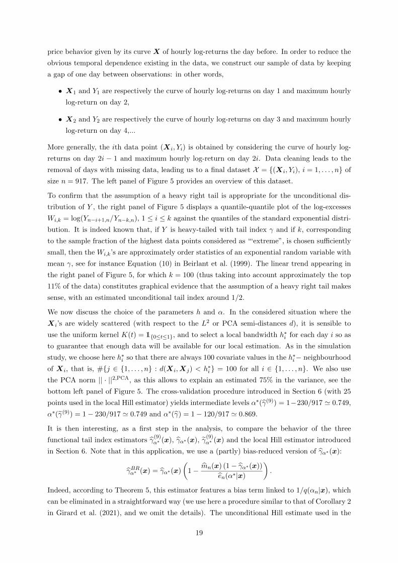
price behavior given by its curve X of hourly log-returns the day before. In order to reduce the
obvious temporal dependence existing in the data, we construct our sample of data by keeping
a gap of one day between observations: in other words,
• X1 and Y1 are respectively the curve of hourly log-returns on day 1 and maximum hourly
log-return on day 2,
• X2 and Y2 are respectively the curve of hourly log-returns on day 3 and maximum hourly
log-return on day 4,...
More generally, the ith data point (Xi, Yi) is obtained by considering the curve of hourly log-
returns on day 2i − 1 and maximum hourly log-return on day 2i. Data cleaning leads to the
removal of days with missing data, leading us to a final dataset X = {(Xi, Yi), i = 1, . . . , n} of
size n = 917. The left panel of Figure 5 provides an overview of this dataset.
To confirm that the assumption of a heavy right tail is appropriate for the unconditional dis-
tribution of Y , the right panel of Figure 5 displays a quantile-quantile plot of the log-excesses
Wi,k = log(Yn−i+1,n/Yn−k,n), 1 ≤ i ≤ k against the quantiles of the standard exponential distri-
bution. It is indeed known that, if Y is heavy-tailed with tail index γ and if k, corresponding
to the sample fraction of the highest data points considered as “‘extreme”, is chosen sufficiently
small, then the Wi,k’s are approximately order statistics of an exponential random variable with
mean γ, see for instance Equation (10) in Beirlant et al. (1999). The linear trend appearing in
the right panel of Figure 5, for which k = 100 (thus taking into account approximately the top
11% of the data) constitutes graphical evidence that the assumption of a heavy right tail makes
sense, with an estimated unconditional tail index around 1/2.
We now discuss the choice of the parameters h and α. In the considered situation where the
Xi’s are widely scattered (with respect to the L2 or PCA semi-distances d), it is sensible to
use the uniform kernel K(t) = 1{0≤t≤1}, and to select a local bandwidth h∗i for each day i so as
to guarantee that enough data will be available for our local estimation. As in the simulation
study, we choose here h∗i so that there are always 100 covariate values in the h∗i− neighbourhood
of Xi, that is, #{j ∈ {1, . . . , n} : d(Xi,Xj) < h∗i } = 100 for all i ∈ {1, . . . , n}. We also use
the PCA norm || · ||2,PCA, as this allows to explain an estimated 75% in the variance, see the
bottom left panel of Figure 5. The cross-validation procedure introduced in Section 6 (with 25
points used in the local Hill estimator) yields intermediate levels α∗(γ(9)) = 1−230/917 ' 0.749,
α∗(γ(9)) = 1− 230/917 ' 0.749 and α∗(γ) = 1− 120/917 ' 0.869.
It is then interesting, as a first step in the analysis, to compare the behavior of the three
functional tail index estimators γ(9)α∗ (x), γα∗(x), γ
(9)α∗ (x) and the local Hill estimator introduced
in Section 6. Note that in this application, we use a (partly) bias-reduced version of γα∗(x):
γBRα∗ (x) = γα∗(x)
(1− mn(x) (1− γα∗(x))
en(α∗|x)
).
Indeed, according to Theorem 5, this estimator features a bias term linked to 1/q(αn|x), which
can be eliminated in a straightforward way (we use here a procedure similar to that of Corollary 2
in Girard et al. (2021), and we omit the details). The unconditional Hill estimate used in the
19

0.0 0.2 0.4 0.6 0.8 1.0
−0.
3−
0.1
0.1
0.3
Bitcoin price log−returns
0 1 2 3 40.
00.
51.
01.
52.
0
QQ−plot
Scree plot
Number of components
Fra
ctio
n of
var
ianc
e ex
plai
ned
1 2 3 4 5 6
0.0
0.2
0.4
0.6
0.8
1.0
Cumul. FVE
Figure 5: Financial data on the price of Bitcoin. Top left panel: Hourly log-returns
of Bitcoin price. Top right panel: Exponential quantile-quantile plot of the log-excesses
log(Yn−i+1,n/Yn−k,n) (vertically) versus log((k+1)/i) (horizontally), for 1 ≤ i ≤ k, with k = 100.
The straight line has a slope computed using the Hill estimator on the top k Yi’s. Bottom panel:
scree plot following the functional PCA procedure, obtained via the FPCA function of the R
package fdapace.
20

QQ-plot of Figure 5 is slightly below 1/2; it is likely, from Theorem 6 and Figure 1, that this is
a favorable case for our proposed estimator γ(9)α∗ (x), due to our estimator having lowest variance
in this area.
Using these selected parameters, our aim is now, for each i ∈ {1, . . . , n}, to predict the expectile
of level βn of Yi, the maximum hourly log-return of the price of Bitcoin on day i+ 1, given Xi,
the curve of hourly log-returns on day i, using the dataset X−i = {(Xj , Yj), j 6= i}. We propose
to consider the extreme level βn = 1 − 1/n ≈ 0.999. To give a reasonable idea of how extreme
conditional expectiles vary in this functional context, we represent the bias-reduced estimated
expectiles eW,BRn,α∗ (βn|Xi) (introduced in Equation (6.1) and improving upon (4.4)), versus the
PCA norm ||Xi||2,PCA and the daily volatility s2(Xi) = mean((Xi − Xi)2) (here Xi denotes
the average hourly log-return) in Figures 6 and 7. One can observe that the expectile curves
seem to increase with respect to both the norm and the volatility, and that all the proposed
estimators return similar values. As a sanity check, we recall that from (4.2), as n→∞, one has
nP (Y > e (1− 1/n|x) |x) → (γ(x)−1 − 1). In this example, based on a value of the functional
tail index around 0.4, we would therefore expect no more than a handful of exceedances above
the estimated conditional expectile eW,BRn,α∗ (βn|Xi) = eW,BRn,α∗ (1−1/n|Xi). A graphical inspection
yields 2 exceedances for the estimate based on γ(9)α∗ (x), and 4 exceedances for the estimates
based on either γ(9)α∗ (x) or γBRα∗ (x). Finally, in order to confirm our previous observation on the
trend of extreme expectiles depending on volatility, we plot in Figure 8 our expectile predictions
sorted by volatility observed the previous day. The estimated expectile curves generally behave
as the observed values of the Yi; in comparison with the other estimates, γBRα∗ (x) seems to lead
to lower estimates of the extreme expectiles. All in all, it appears that our extreme expectile
method gives a reasonable account of large movements in the price of Bitcoin; they in particular
give an indication that a large volatility on a given day leads to potentially more extreme swings
in price the following day.
Acknowledgements
The authors acknowledge an anonymous Associate Editor and an anonymous reviewer for their
comments that led to an improved version of this paper. This research was supported by
the French National Research Agency under the grant ANR-19-CE40-0013/ExtremReg project.
S. Girard gratefully acknowledges the support of the Chair Stress Test, Risk Management and
Financial Steering, led by the French Ecole Polytechnique and its Foundation and sponsored
by BNP Paribas, and the support of the French National Research Agency in the framework
of the Investissements d’Avenir programme (ANR-15-IDEX-02). G. Stupfler also acknowledges
support from an AXA Research Fund Award on “Mitigating risk in the wake of the COVID-19
pandemic”.
21

0.000 0.004 0.008
0.0
0.2
0.4
0.6
Expectile estimators
0.000 0.004 0.0080.
00.
20.
40.
6
Tail index estimators
0.000 0.002 0.004
0.0
0.2
0.4
0.6
Expectile estimators
0.000 0.002 0.004
0.0
0.2
0.4
0.6
Tail index estimators
Figure 6: Left panels: Direct expectile estimates eW,BRn,α∗ (βn|·) based on the four tail index es-
timators γ(9)αn (·) (red), γBRα∗ (·) (green), γ
(9)αn (·) (blue) and a local Hill estimator (brown). Right
panels: Tail index estimates, with the same color code. On all panels, curves are smoothed
with the R function loess (and a smoothing parameter of 0.25). The black dots are the pairs(||Xi||2,PCA, Yi
). The bottom panels zoom in on the region ||x||2,PCA ∈ [0, 0.005].
22

0.0000 0.0010 0.0020
0.0
0.2
0.4
0.6
Expectile estimators
0.0000 0.0010 0.00200.
00.
20.
40.
6
Tail index estimators
0e+00 2e−04 4e−04
0.0
0.2
0.4
0.6
Expectile estimators
0e+00 2e−04 4e−04
0.0
0.2
0.4
0.6
Tail index estimators
Figure 7: Left panels: Direct expectile estimates eW,BRn,α∗ (βn|·) based on the four tail index es-
timators γ(9)αn (·) (red), γBRα∗ (·) (green), γ
(9)αn (·) (blue) and a local Hill estimator (brown). Right
panels: Tail index estimates, with the same color code. On all panels, curves are smoothed
with the R function loess (and a smoothing parameter of 0.25). The black dots are the pairs(s2(Xi), Yi
). The bottom panels zoom in on the region s2(x) ∈ [0, 0.0005].
23

0 200 400 600 800
0.0
0.2
0.4
0.6
0.8
1.0
0 200 400 600 800
0.0
0.2
0.4
0.6
0.8
1.0
0 200 400 600 800
0.0
0.2
0.4
0.6
0.8
1.0
0 200 400 600 800
0.0
0.2
0.4
0.6
0.8
1.0
Figure 8: Extreme expectile estimates eW,BRn,α∗ (βn|Xi) based on γ(9)αn (·) (top left), γBRα∗ (·) (top
right), γ(9)αn (·) (bottom left) and a local Hill estimator (bottom right). The black curves represent
the pairs (ji, Yji), where the ji are such that s2(Xj1) < · · · < s2(Xjn), and the colored curves
represent the predicted extreme expectiles (ji, eW,BRn,α∗ (βn|Xji)).
24
References
Acerbi, C. (2002). Spectral measures of risk: A coherent representation of subjective risk
aversion. Journal of Banking & Finance, 26(7):1505–1518.
Artzner, P., Delbaen, F., Eber, J.-M., and Heath, D. (1999). Coherent measures of risk. Math-
ematical Finance, 9(3):203–228.
Beirlant, J., Dierckx, G., Goegebeur, Y., and Matthys, G. (1999). Tail index estimation and an
exponential regression model. Extremes, 2(2):177–200.
Bellini, F., Klar, B., Muller, A., and Gianin, E. R. (2014). Generalized quantiles as risk measures.
Insurance: Mathematics and Economics, 54:41–48.
Berlinet, A., Gannoun, A., and Matzner-Løber, E. (2001). Asymptotic normality of convergent
estimates of conditional quantiles. Statistics, 35(2):139–169.
Billingsley, P. (1995). Probability and Measure (Third edition). John Wiley & Sons.
Bingham, N. H., Goldie, C. M., and Teugels, J. L. (1989). Regular Variation. Cambridge
University Press.
Breckling, J. and Chambers, R. (1988). M-quantiles. Biometrika, 75(4):761–771.
Cai, J. and Weng, C. (2016). Optimal reinsurance with expectile. Scandinavian Actuarial
Journal, 2016(7):624–645.
Carroll, C., Gajardo, A., Chen, Y., Dai, X., Fan, J., Hadjipantelis, P. Z., Han, K., Ji, H.,
Mueller, H.-G., and Wang, J.-L. (2021). fdapace: Functional Data Analysis and Empirical
Dynamics. R package version 0.5.6.
Chang, J. T. and Pollard, D. (1997). Conditioning as disintegration. Statistica Neerlandica,
51(3):287–317.
Chen, Z. (1996). Conditional Lp-quantiles and their application to the testing of symmetry in
non-parametric regression. Statistics & Probability Letters, 29(2):107–115.
Daouia, A., Gardes, L., and Girard, S. (2013). On kernel smoothing for extremal quantile
regression. Bernoulli, 19(5B):2557–2589.
Daouia, A., Gardes, L., Girard, S., and Lekina, A. (2011). Kernel estimators of extreme level
curves. TEST, 20:311–333.
Daouia, A., Girard, S., and Stupfler, G. (2018). Estimation of tail risk based on extreme
expectiles. Journal of the Royal Statistical Society: Series B, 80(2):263–292.
Daouia, A., Girard, S., and Stupfler, G. (2019). Extreme M-quantiles as risk measures: from L1
to Lp optimization. Bernoulli, 25(1):264–309.
25

Daouia, A., Girard, S., and Stupfler, G. (2020). Tail expectile process and risk assessment.
Bernoulli, 26(1):531–556.
de Haan, L. and Ferreira, A. (2006). Extreme Value Theory: An Introduction. Springer-Verlag,
New York.
El Methni, J., Gardes, L., and Girard, S. (2014). Non-parametric estimation of extreme risk
measures from conditional heavy-tailed distributions. Scandinavian Journal of Statistics,
41(4):988–1012.
Embrechts, P., Kluppelberg, C., and Mikosch, T. (1997). Modelling Extremal Events for Insur-
ance and Finance. Springer.
Ferraty, F., Laksaci, A., and Vieu, P. (2006). Estimating some characteristics of the conditional
distribution in nonparametric functional models. Statistical Inference for Stochastic Processes,
9(1):47–76.
Ferraty, F., Mas, A., and Vieu, P. (2007). Nonparametric regression on functional data: inference
and practical aspects. Australian & New Zealand Journal of Statistics, 49(3):267–286.
Ferraty, F., Rabhi, A., and Vieu, P. (2005). Conditional quantiles for dependent functional
data with application to the climatic El Nino phenomenon. Sankhya: The Indian Journal of
Statistics, 67(2):378–398.
Ferraty, F. and Vieu, P. (2006). Nonparametric Functional Data Analysis. Springer.
Gannoun, A. (1990). Estimation non parametrique de la mediane conditionnelle.
Medianogramme et methode du noyau. Application A la prevision des processus. Publi-
cations de l’Institut de Statistique de l’Universite de Paris, XXXV(1):11–22.
Gardes, L. and Girard, S. (2012). Functional kernel estimators of large conditional quantiles.
Electronic Journal of Statistics, 6:1715–1744.
Gardes, L. and Stupfler, G. (2014). Estimation of the conditional tail index using a smoothed
local Hill estimator. Extremes, 17(1):45–75.
Gardes, L. and Stupfler, G. (2019). An integrated functional Weissman estimator for conditional
extreme quantiles. REVSTAT: Statistical Journal, 17(1):109–144.
Girard, S., Stupfler, G., and Usseglio-Carleve, A. (2021). Nonparametric extreme conditional
expectile estimation. Scandinavian Journal of Statistics. To appear.
Gneiting, T. (2011). Making and evaluating point forecasts. Journal of the American Statistical
Association, 106(494):746–762.
Hill, B. M. (1975). A simple general approach to inference about the tail of a distribution. The
Annals of Statistics, 3(5):1163–1174.
26

Jones, M. C. (1994). Expectiles and M-quantiles are quantiles. Statistics & Probability Letters,
20(2):149–153.
Kato, K. (2012). Estimation in functional linear quantile regression. The Annals of Statistics,
40(6):3108–3136.
Koenker, R. and Bassett, G. J. (1978). Regression quantiles. Econometrica, 46(1):33–50.
Krzyzak, A. (1986). The rates of convergence of kernel regression estimates and classification
rules. IEEE Transactions on Information Theory, 32(5):668–679.
Kuan, C.-M., Yeh, J.-H., and Hsu, Y.-C. (2009). Assessing value at risk with care, the conditional
autoregressive expectile models. Journal of Econometrics, 150(2):261–270.
Li, W. V. and Shao, Q.-M. (2001). Gaussian processes: inequalities, small ball probabilities
and applications. In Rao, C. and Shanbhag, D., editors, Stochastic processes, Theory and
Methods. Handbook of Statistics, volume 19, pages 533–597. Elsevier, Amsterdam.
Metwally, S. A. and Atiya, A. F. (2002). Using Brownian bridge for fast simulation of jump-
diffusion processes and barrier options. Journal of Derivatives, 10(1):43–54.
Newey, W. K. and Powell, J. L. (1987). Asymmetric least squares estimation and testing.
Econometrica, 55(4):819–847.
Pickands, J. (1975). Statistical inference using extreme order statistics. The Annals of Statistics,
3(1):119–131.
Resnick, S. (2007). Heavy-Tail Phenomena: Probabilistic and Statistical Modeling. Springer.
Samanta, M. (1989). Non-parametric estimation of conditional quantiles. Statistics & Probability
Letters, 7(5):407–412.
Stone, C. J. (1977). Consistent nonparametric regression (with discussion). The Annals of
Statistics, 5(4):595–645.
Stupfler, G. (2013). A moment estimator for the conditional extreme-value index. Electronic
Journal of Statistics, 7:2298–2343.
Stupfler, G. (2016). Estimating the conditional extreme-value index under random right-
censoring. Journal of Multivariate Analysis, 144:1–24.
Stute, W. (1986). Conditional empirical processes. The Annals of Statistics, 14(2):638–647.
Taylor, J. W. (2008). Estimating Value at Risk and Expected Shortfall Using Expectiles. Journal
of Financial Econometrics, 6(2):231–252.
Weissman, I. (1978). Estimation of parameters and large quantiles based on the k largest
observations. Journal of the American Statistical Association, 73(364):812–815.
Ziegel, J. (2016). Coherence and elicitability. Mathematical Finance, 26(4):901–918.
27

A Appendix: proofs
This Appendix is organized as follows: Section A.1 provides some preliminary results useful for
the proofs of the main results in Section A.2. Define
ψ(k)n (y|x) =
1
n
n∑i=1
(Yi − y)kK
(d (x,Xi)
hn
)1{Yi>y}
/µ
(1)K (x, hn)
and m(k)n (y|x) =
1
n
n∑i=1
(Yi − y)k K
(d (x,Xi)
hn
)/µ
(1)K (x, hn).
The quantities ψ(k)n (y|x) and m
(k)n (y|x) are the pseudo-estimator counterparts of ψ
(k)n (y|x) and
m(k)n (y|x) when the smoothed small-ball probability µ
(1)K (x, hn) is assumed to be known.
A.1 Preliminary results
Lemma 1. Assume that (K) holds. Then for any x ∈ E, h > 0 and b > 0,
cb1π(x, h) ≤ µ(b)K (x, h) ≤ cb2π(x, h).
In particular, for any b, b′ > 0 and δ > 0, [µ(b′)K (x, h)]1+δ/µ
(b)K (x, h)→ 0 as h→ 0.
Proof. The double inequality is an obvious consequence of assumption (K). The desired conver-
gence follows because, by monotone convergence, π(x, h)→ P(X = x) = 0 as h→ 0 (since the
probability distribution of X is non-atomic).
Lemma 2. Assume that (L) holds. Let yn →∞ and hn → 0. Then, uniformly in x′ ∈ B(x, hn),
m(1)(yn|x′)−m(1)(yn|x) = O(hn) and m(2)(yn|x′)−m(2)(yn|x) = O(ynhn).
Proof. Remarking that
m(1)(yn|x′)−m(1)(yn|x) = m(1)(0|x′)−m(1)(0|x),
m(2)(yn|x′)−m(2)(yn|x) = m(2)(0|x′)−m(2)(0|x)− 2yn
(m(1)(0|x′)−m(1)(0|x)
),
the result is a straightforward consequence of (L).
Lemma 3. Assume (K) holds. Let yn →∞ and hn → 0 be such that nπ(x, hn)→∞ as n→∞.
Then,
E[m(0)n (yn|x)
]= 1 and Var
[m(0)n (yn|x)
]=
µ(2)K (x, hn)
nµ(1)K (x, hn)2
(1 + o(1)).
If moreover (L) holds then
E[m(1)n (yn|x)
]= m(1)(yn|x)+O(hn) and Var
[m(1)n (yn|x)
]=
µ(2)K (x, hn)
nµ(1)K (x, hn)2
m(2)(yn|x)(1+o(1)).
28

Proof. By definition,
E[m(0)n (yn|x)
]=
E[K(d(x,X)hn
)]µ
(1)K (x, hn)
= 1,
hence the first result. The second one is obtained through a similar calculation:
Var[m(0)n (yn|x)
]=
E[K2(d(x,X)hn
)]−(E[K(d(x,X)hn
)])2
nµ(1)K (x, hn)2
=µ
(2)K (x, hn)− µ(1)
K (x, hn)2
nµ(1)K (x, hn)2
.
Using Lemma 1 proves the result. Then,
E[m(1)n (yn|x)
]=
E[m(1)(yn|X)K
(d(x,X)hn
)]µ
(1)K (x, hn)
= m(1)(yn|x) +O(hn)
from Lemma 2. The third result is proved. The fourth one is obtained through a similar
calculation:
Var[m(1)n (yn|x)
]=
E[(m(2)(yn|X)−m(2)(yn|x)
)K(d(x,X)hn
)2]
+m(2)(yn|x)µ(2)K (x, hn)
nµ(1)K (x, hn)2
− m(1)(yn|x)2
n(1 + o(1)).
Clearly m(1)(yn|x) = yn(1 + o(1)) and m(2)(yn|x) = y2n(1 + o(1)). Combining the results of
Lemmas 1 and 2 concludes the proof.
In the next lemma and throughout, B(·, ·) denotes the Beta function. The proofs of Lemmas 4
and 5 are omitted: they are straightforward adaptations of corresponding results (Lemma 2i) and
Lemma 3 respectively) in Girard et al. (2021), whose proofs are written based on a multivariate
covariate (their finite-dimensional nature not playing any role whatsoever).
Lemma 4. Suppose C1(γ(x)) holds. Then, for all a ∈ [0, 1/γ(x)),
ψ(a)(y|x) =B(a+ 1, γ(x)−1 − a
)γ(x)
yaF (y|x)(1 + o(1)) as y →∞.
Lemma 5. Assume C1(γ(x)) holds. Let yn →∞ and hn → 0 such that ωhn(yn|x) log(yn)→ 0.
Then, uniformly in x′ ∈ B(x, hn) and for all a ∈ [0, 1/γ(x)),
ψ(a)(yn|x′)ψ(a)(yn|x)
− 1 = O(ωhn(yn|x) log(yn)).
Lemma 6. Assume that (K) and C1(γ(x)) hold. Let yn → ∞ and hn → 0 be such that
ωhn(yn|x) log(yn)→ 0 as n→∞. Then, for all a ∈ [0, 1/γ(x)) and b > 0,
E[(Y − yn)aKb
(d (x,X)
hn
)1{Y >yn}
]= ψ(a)(yn|x)µ
(b)K (x, hn)(1 +O(ωhn(yn|x) log(yn))).
In particular,
∀a ∈ [0, 1/γ(x)), E[ψ(a)n (yn|x)
]= ψ(a)(yn|x) (1 +O (ωhn(yn|x) log(yn)))
and ∀a ∈ [0, 1/(2γ(x))), Var[ψ(a)n (yn|x)
]= ψ(2a)(yn|x)
(µ
(2)K (x, hn)
nµ(1)K (x, hn)2
)(1 + o(1)).
29

Proof. The first identity is immediate by noting that
E[(Y − yn)aKb
(d (x,X)
hn
)1{Y >yn}
]= E
[ψ(a)(yn|X)Kb
(d (x,X)
hn
)]and applying Lemma 5. The second one follows immediately because
E[ψ(a)n (yn|x)
]=
1
µ(1)K (x, hn)
E[(Y − yn)aK
(d (x,X)
hn
)1{Y >yn}
].
The third result can be obtained by similar calculations, which yield
Var[ψ(a)n (yn|x)
]=ψ(2a)(yn|x)µ
(2)K (x, hn)
nµ(1)K (x, hn)2
(1 + o(1))− ψ(a)(yn|x)2
n(1 + o(1)),
Combining the results of Lemmas 1 and 4 completes the proof.
Lemma 7. Assume (K) and C1(γ(x)) hold with γ(x) < 1/2. Suppose also that there exists
δ ∈ (0, 1) such that E[Y 2+δ− |X = x] < ∞. Let yn → ∞, hn → 0 and zn = θyn(1 + o(1)), with
θ > 0, such that nF (yn|x)π(x, hn)→∞ and√nF (yn|x)π(x, hn) log(yn)ωhn ((1− δ)(θ ∧ 1)yn|x)→ 0.
If, for all j ∈ {1, . . . , J}, yn,j = τ−γ(x)j yn(1 + o(1)) with 0 < τ1 < τ2 < . . . < τJ ≤ 1, then√√√√nF (yn|x)
µ(1)K (x, hn)2
µ(2)K (x, hn)
(ψ
(1)n (yn,j |x)
ψ(1)(yn,j |x)− 1
)1≤j≤J
,
(ψ
(0)n (zn|x)
ψ(0)(zn|x)− 1
) d−→ N (0J+1,V (x))
where V (x) is the symmetric matrix having entries:
Vj,l(x) =1− γ(x)
γ(x)τ−1l
[1
1− 2γ(x)
(τjτl
)−γ(x)
− 1
], (j, l) ∈ {1, . . . , J}2, j ≤ l,
Vj,J+1(x) =γ(x)θ1/γ(x)
(θ ∨ τ−γ(x)
j
)1−1/γ(x)+ (1− γ(x))
(θ ∨ τ−γ(x)
j − τ−γ(x)j
)γ(x)τ
1−γ(x)j
, j ∈ {1, . . . , J},
VJ+1,J+1(x) = θ1/γ(x).
If in addition (L) holds, then√√√√nF (yn|x)µ
(1)K (x, hn)2
µ(2)K (x, hn)
(En(yn,j |x)
E(yn,j |x)− 1
)1≤j≤J
,
(Fn(zn|x)
F (zn|x)− 1
) d−→ N (0J+1,V (x)) .
Proof. Let β = (β1, . . . , βJ , βJ+1) ∈ RJ+1 and vn(x) =
√nF (yn|x)
µ(1)K (x,hn)2
µ(2)K (x,hn)
. One has:
vn(x)
J∑j=1
βj
(ψ
(1)n (yn,j |x)
ψ(1)(yn,j |x)− 1
)+ βJ+1
(ψ
(0)n (zn|x)
ψ(0)(zn|x)− 1
)= vn(x)
J∑j=1
βj
ψ(1)n (yn,j |x)− E
[ψ
(1)n (yn,j |x)
]ψ(1)(yn,j |x)
+ βJ+1
ψ(0)n (zn|x)− E
[ψ
(0)n (zn|x)
]ψ(0)(zn|x)
+ vn(x)
J∑j=1
βj
E[ψ
(1)n (yn,j |x)
]ψ(1)(yn,j |x)
− 1
+ βJ+1
E[ψ
(0)n (zn|x)
]ψ(0)(zn|x)
− 1
.
30

According to Lemma 6, E[ψ
(0)n (zn|x)
]= ψ(0)(zn|x)(1 +O(ωhn(zn|x) log(zn))),
E[ψ
(1)n (yn,j |x)
]= ψ(1)(yn,j |x)(1 +O(ωhn(yn,j |x) log(yn,j))).
Noticing that for n large enough, yn,j > yn(1 − δ), we obtain ωhn(yn,j |x) ≤ ωhn((1 − δ)yn|x),
∀j ∈ {1, . . . , J}. Similarly zn > θyn(1− δ) and thus ωhn(zn|x) ≤ ωhn((1− δ)θyn|x). Moreover,
log(yn,j) = O(log(yn)) for any j ∈ {1, . . . , J} and log(zn) = O(log(yn)). Therefore
vn(x)
J∑j=1
βj
E[ψ
(1)n (yn,j |x)
]ψ(1)(yn,j |x)
− 1
+ βJ+1
E[ψ
(0)n (zn|x)
]ψ(0)(zn|x)
− 1
= o(1).
We now focus on the asymptotic distribution of
Zn = vn(x)
J∑j=1
βj
ψ(1)n (yn,j |x)− E
[ψ
(1)n (yn,j |x)
]ψ(1)(yn,j |x)
+ βJ+1
ψ(0)n (zn|x)− E
[ψ
(0)n (zn|x)
]ψ(0)(zn|x)
.
We clearly have E[Zn] = 0. In addition, Var[Zn] = F (yn|x)β>B(n)β, where B(n) is the sym-
metric matrix-valued sequence having entries
B(n)j,l =
cov(
(Y − yn,j)K(d(x,X)hn
)1{Y >yn,j}, (Y − yn,l)K
(d(x,X)hn
)1{Y >yn,l}
)µ
(2)K (x, hn)ψ(1)(yn,j |x)ψ(1)(yn,l|x)
, j ≤ l ∈ {1, . . . , J},
B(n)j,J+1 =
cov(
(Y − yn,j)K(d(x,X)hn
)1{Y >yn,j},K
(d(x,X)hn
)1{Y >zn}
)µ
(2)K (x, hn)ψ(1)(yn,j |x)ψ(0)(zn|x)
, j ∈ {1, . . . , J},
B(n)J+1,J+1 =
Var[K(d(x,X)hn
)1{Y >zn}
]µ
(2)K (x, hn)[ψ(0)(zn|x)]2
.
Let us first focus, for j ≤ l, on the term A(n)j,l = B
(n)j,l ψ
(1)(yn,j |x)ψ(1)(yn,l|x). Since yn,j > yn,l
for n large enough, we find:
A(n)j,l =
1
µ(2)K (x, hn)
E[(Y − yn,j)(Y − yn,l)K2
(d(x,X)
hn
)1{Y >yn,j}
]− 1
µ(2)K (x, hn)
E[(Y − yn,j)K
(d(x,X)
hn
)1{Y >yn,j}
]E[(Y − yn,l)K
(d(x,X)
hn
)1{Y >yn,l}
].
According to Lemma 6, the second term is equal to µ(1)K (x, hn)2ψ(1)(yn,j |x)ψ(1)(yn,l|x)/µ
(2)K (x, hn)(1+
o(1)). It thus remains to focus on the first term of A(n)j,l which we rewrite as
1
µ(2)K (x, hn)
(E[(Y − yn,j)2K2
(d(x,X)
hn
)1{Y >yn,j}
]+ (yn,j − yn,l)E
[(Y − yn,j)K2
(d(x,X)
hn
)1{Y >yn,j}
]).
Using Lemma 6, we get
1
µ(2)K (x, hn)
E[(Y − yn,j)2K2
(d(x,X)
hn
)1{Y >yn,j}
]= ψ(2)(yn,j |x)(1 + o(1))
31

and
(yn,j − yn,l)µ
(2)K (x, hn)
E[(Y − yn,j)K2
(d(x,X)
hn
)1{Y >yn,j}
]=(τ−γ(x)j − τ−γ(x)
l
)ψ(1)(yn,j |x)yn(1+o(1)).
Besides, Lemma 4 and the regular variation property of F (·|x) provide, for any j,ψ(1)(yn,j |x) =
γ(x)
1− γ(x)τ−γ(x)j ynτjF (yn|x)(1 + o(1)),
ψ(2)(yn,j |x) =2γ(x)2
(1− 2γ(x))(1− γ(x))τ−2γ(x)j y2
nτjF (yn|x)(1 + o(1)).
Consequently the first term in A(n)j,l is of order y2
nF (yn|x) and thus dominates, by Lemma 1.
Straightforward calculations then yield:
B(n)j,l =
1− γ(x)
γ(x)τ−1l
[1
1− 2γ(x)
τ−γ(x)j
τ−γ(x)l
− 1
]1
F (yn|x)(1 + o(1)).
We now deal with B(n)j,J+1 for j ∈ {1, . . . , J}, which can be rewritten as
E[(Y − yn,j)K2
(d(x,X)hn
)1{Y >yn,j∨zn}
]− E
[(Y − yn,j)K
(d(x,X)hn
)1{Y >yn,j}
]E[K(d(x,X)hn
)1{Y >zn}
]µ
(2)K (x, hn)ψ(1)(yn,j |x)ψ(0)(zn|x)
.
Using Lemma 6, the second term in the numerator equals µ(1)K (x, hn)2ψ(1)(yn,j |x)ψ(0)(zn|x)(1 +
o(1)) and the first term can be rewritten
E[(Y − yn,j)K2
(d(x,X)
hn
)1{Y >yn,j∨zn}
]= µ
(2)K (x, hn)
[ψ(1)(yn,j ∨ zn|x) + (yn,j ∨ zn − yn,j)ψ(0)(yn,j ∨ zn|x)
](1 + o(1)).
Combining Lemma 1 and Lemma 4 with the asymptotic equivalent F (yn,j ∨ zn|x)/F (yn|x) =
(θ ∨ τ−γ(x)j )−1/γ(x)(1 + o(1)), we get that the first term dominates again. From straightforward
calculations,
B(n)j,J+1 =
ψ(1)(yn,j ∨ zn|x) + (yn,j ∨ zn − yn,j)ψ(0)(yn,j ∨ zn|x)
ψ(1)(yn,j |x)ψ(0)(zn|x)(1 + o(1))
=γ(x)
(θ ∨ τ−γ(x)
j
)1−1/γ(x)+ (1− γ(x))
(θ ∨ τ−γ(x)
j − τ−γ(x)j
)(θ ∨ τ−γ(x)
j
)−1/γ(x)
γ(x)τ1−γ(x)j θ−1/γ(x)
1
F (yn|x)(1 + o(1))
=γ(x)
(θ ∨ τ−γ(x)
j
)1−1/γ(x)+ (1− γ(x))
(θ ∨ τ−γ(x)
j − τ−γ(x)j
)θ−1/γ(x)
γ(x)τ1−γ(x)j θ−1/γ(x)
1
F (yn|x)(1 + o(1)).
Finally, combining Lemmas 1, 4 and 6, the variance term B(n)J+1,J+1 is clearly
E[K2(d(x,X)hn
)1{Y >zn}
]−{E[K(d(x,X)hn
)1{Y >zn}
]}2
µ(2)K (x, hn)[ψ(0)(zn|x)]2
= θ1/γ(x) 1
F (yn|x)(1 + o(1)).
32

Therefore, Var[Zn] → β>V (x)β, where V (x) is given in the statement of the lemma. It only
remains to prove the asymptotic normality of Zn. We thus write Zn =∑n
i=1 Zi,n, where
Zi,n =vn(x)
nµ(1)K (x, hn)
J∑j=1
βj(Yi − yn,j)K
(d(x,Xi)hn
)1{Yi>yn,j} − E
[(Yi − yn,j)K
(d(x,Xi)hn
)1{Yi>yn,j}
]ψ(1)(yn,j |x)
+vn(x)
nµ(1)K (x, hn)
βJ+1
K(d(x,Xi)hn
)1{Yi>zn} − E
[K(d(x,Xi)hn
)1{Yi>zn}
]ψ(0)(zn|x)
.
We prove that there is δ > 0 such that nE|Z1,n|2+δ → 0 as n → ∞; the result then follows
by the Lyapunov central limit theorem (see Theorem 27.3 p.362 of Billingsley, 1995). For that
purpose, note that, if T1, . . . , Tq have finite (2 + δ)−moments,E
∣∣∣∣∣q∑i=1
[Ti − E(Ti)]
∣∣∣∣∣2+δ
1/(2+δ)
≤q∑i=1
{E|Ti|2+δ}1/(2+δ) + E|Ti| ≤ 2q max1≤i≤q
{E|Ti|2+δ}1/(2+δ)
by the triangle inequality for the standard norm in the space of random variables with finite
(2 + δ)−moment, and Jensen’s inequality. Therefore, E|Z1,n|2+δ =
O
( F (yn|x)
nµ(2)K (x, hn)
)1+δ/2 max
1≤j≤JE
∣∣∣∣∣∣(Y − yn,j)K
(d(x,X)hn
)1{Y >yn,j}
ψ(1)(yn,j |x)
∣∣∣∣∣∣2+δ
+ E
∣∣∣∣∣∣K(d(x,X)hn
)1{Y >zn}
ψ(0)(zn|x)
∣∣∣∣∣∣2+δ .
Combine now, for δ small enough, Lemmas 1, 4 and 6 with the asymptotic equivalences F (zn|x) =
θ−1/γ(x)F (yn|x)(1 + o(1)) and F (yn,j |x) = τjF (yn|x)(1 + o(1)) to get
nE|Z1,n|2+δ = O([nπ(x, hn)F (yn|x)
]−δ/2),
which clearly tends to 0 as n→∞. The first result is proved. To show the second result, set
Rn,j :=2(ψ
(1)n (yn,j |x)− ψ(1)(yn,j |x)
)−(m
(1)n (yn,j |x)−m(1)(yn,j |x)
)2ψ(1)(yn,j |x)−m(1)(yn,j |x)
.
We may write
vn(x)
J∑j=1
βj
(En(yn,j |x)
E(yn,j |x)− 1
)+ vn(x)βJ+1
(Fn(zn|x)
F (zn|x)− 1
)
= vn(x)
J∑j=1
βj
(ψ
(1)n (yn,j |x)
ψ(1)(yn,j |x)− 1
)(1 +Rn,j)
−1 + vn(x)βJ+1
(ψ
(0)n (zn|x)
ψ(0)(zn|x)− 1
)1
m(0)n (zn|x)
+ vn(x)
J∑j=1
βj((1 +Rn,j)
−1 − 1)
+ vn(x)βJ+1
(1
m(0)n (zn|x)
− 1
).
Combining Lemmas 1, 3 and 6 directly entails
∀j ∈ {1, . . . , J}, Rn,j = OP
(1√
nπ(x, hn)
)= oP
1√nπ(x, hn)F (yn|x)
P−→ 0
and the result then follows by applying the first result of the lemma.
33

Lemma 8. Assume (K) and C1(γ(x)) hold. Let yn →∞, hn → 0 and zn = θyn(1 + o(1)), with
θ > 0, be such that nF (yn|x)π(x, hn)→∞ and
∃δ > 0,√nF (yn|x)π(x, hn) log(yn)ωhn((1− δ)(θ ∧ 1)yn|x)→ 0.
Then if, for all j ∈ {1, . . . , J}, yn,j = τ−γ(x)j yn(1 + o(1)) with 0 < τ1 < τ2 < . . . < τJ ≤ 1, one
has√√√√nF (yn|x)µ
(1)K (x, hn)2
µ(2)K (x, hn)
(Fn(yn,j |x)
F (yn,j |x)− 1
)1≤j≤J
,
(Fn(zn|x)
F (zn|x)− 1
) d−→ N (0J+1,Σ(x)) ,
where Σ(x) is the symmetric matrix having entries:Σj,l(x) = τ−1
l , (j, l) ∈ {1, . . . , J}2, j ≤ l,
Σj,J+1(x) =(τj ∨ θ−1/γ(x)
)−1, j ∈ {1, . . . , J},
ΣJ+1,J+1(x) = θ1/γ(x).
Proof. The proof is entirely similar to that of Lemma 7 and is thus omitted.
A.2 Proofs of main results
Proof of Theorem 1 Let us recall that σ−1n (x) =
√n(1− αn)
µ(1)K (x,hn)2
µ(2)K (x,hn)
, introduce z =
(z1, . . . , zJ , t) and focus on the probability
Φn(z) = P
J⋂j=1
{σ−1n (x)
(en(αn,j |x)
e(αn,j |x)− 1
)≤ zj
}∩{σ−1n (x)
(qn(an|x)
q(an|x)− 1
)≤ t}
= P
J⋂j=1
{en(αn,j |x) ≤ e(αn,j |x) (1 + zjσn(x))} ∩ {qn(an|x) ≤ q(an|x) (1 + tσn(x))}
.
By noticing that 1−αn,j = E(e(αn,j |x)|x) and 1− an = F (q(an|x)|x), and using that for all y,
α, en(α|x) ≤ y ⇔ En(y|x) ≤ 1− α and qn(α|x) ≤ y ⇔ Fn(y|x) ≤ 1− α, we find that Φn(z) is
equal to
P
J⋂j=1
{En(e(αn,j |x)(1 + zjσn(x))|x) ≤ E(e(αn,j |x)|x)
}∩{Fn(q(an|x)(1 + tσn(x))|x) ≤ F (q(an|x)|x)
} .
Letting yn = e(αn|x), yn,j = e(αn,j |x)(1 + zjσn(x)), zn = q(an|x)(1 + tσn(x)) and vn(x) =√nF (yn|x)
µ(1)K (x,hn)2
µ(2)K (x,hn)
, we have
Φn(z) = P
J⋂j=1
{vn(x)
(En(yn,j |x)
E(yn,j |x)− 1
)≤ vn(x)
(E(e(αn,j |x)|x)
E(yn,j |x)− 1
)}⋂{
vn(x)
(Fn(zn|x)
F (zn|x)− 1
)≤ vn(x)
(F (q(an|x)|x)
F (zn|x)− 1
)}).
34

By Corollary 3 of Girard et al. (2021), E(·|x) is continuously differentiable with
limy→∞
yE′(y|x)
E(y|x)= lim
y→∞
yF′(y|x)
F (y|x)= − 1
γ(x).
Thus, for any j ∈ {1, . . . , J}, a Taylor expansion shows that there exists θn,j ∈ [0, 1] with:
E(yn,j |x) = 1− αn,j + zjσn(x)e(αn,j |x)E′(e(αn,j |x) + θn,jzjσn(x)e(αn,j |x)|x)
= 1− αn,j + zjσn(x)e(αn,j |x)E′(e(αn,j |x)|x)(1 + o(1))
= (1− αn,j)(
1− zjσn(x)
γ(x)(1 + o(1))
)= E(e(αn,j |x)|x)
(1− zjσn(x)
γ(x)(1 + o(1))
).
In view of (4.2), vn(x) = σ−1n (x)
√γ(x)−1 − 1(1 + o(1)) and therefore
∀j ∈ {1, . . . , J}, vn(x)
(E(e(αn,j |x)|x)
E(yn,j |x)− 1
)=
zjγ(x)
√1− γ(x)
γ(x)(1 + o(1)).
Similarly
vn(x)
(F (q(an|x)|x)
F (zn|x)− 1
)=
t
γ(x)
√1− γ(x)
γ(x)(1 + o(1)).
Finally, yn,j = τ−γ(x)j yn(1 + o(1)) and zn =
(γ(x)−1 − 1
)γ(x)τ−γ(x)yn(1 + o(1)), since, in
view of (4.3), e(·|x) is regularly varying. Thus, for n large enough, ωhn(yn,j |x) ≤ ωhn((1 −δ)e(αn|x)|x) and ωhn(zn|x) ≤ ωhn((1 − δ)q(an|x)|x). Moreover, log(yn,j) = O(log(yn)) and
log(zn) = O(log(yn)). Noting that log(yn) = O(| log(1 − αn)|) by the regular variation prop-
erty of the tail expectile function t 7→ e(1 − t−1|x), Lemma 7 can then be applied with
θ = τ−γ(x)(γ(x)−1 − 1
)γ(x)to conclude the proof. 2
Proof of Theorem 2 The key is to write
log
(eWn,αn(βn|x)
e(βn|x)
)= log
(1− αn1− βn
)(γαn(x)−γ(x))+log
(en(αn|x)
e(αn|x)
)+log
([1− αn1− βn
]γ(x) e(αn|x)
e(βn|x)
).
The first term is controlled by our assumptions on γαn(x), the second term by Theorem 1 and
the third one by Lemma 8 of Girard et al. (2021) (whose proof carries over to the functional
case without modification). The delta-method concludes the proof. 2
Proof of Theorem 3 The key is to write
log
(eWn,αn(βn|x)
e(βn|x)
)= log
(1− αn1− βn
)(γαn(x)− γ(x)) + log
(qn(αn|x)
q(αn|x)
)
+ log
([1− αn1− βn
]γ(x) q(αn|x)
q(βn|x)
)
+ log
((γαn(x)−1 − 1
)−γαn (x)
(γ(x)−1 − 1)−γ(x)
)+ log
(q(βn|x)
(γ(x)−1 − 1
)−γ(x)
e(βn|x)
).
Under our conditions, the second term is a OP(σn(x)). According to Theorem 4.3.8 in de Haan
and Ferreira (2006) and condition iii), the third term is a O(A((1− αn)−1|x
))). Similarly,
Proposition 1 in Daouia et al. (2018) entails that the last term is a O(A((1− αn)−1|x
))+
O(q(αn|x)−1
). Finally, our assumptions on γαn(x) imply that the fourth term is a OP(σn(x)).
The result follows. 2
35

Extension and proof of Theorem 4 The proof of Theorem 4 hinges on the result below.
Recall that σn(x) = 1/
√n(1− αn)
µ(1)K (x,hn)2
µ(2)K (x,hn)
.
Proposition 1. Assume (K) and C1(γ(x)) hold. Let αn → 1, hn → 0 and 1 − an = τ(1 −αn)(1 + o(1)) be such that n(1− αn)π(x, hn)→∞ and
∃δ > 0,√n(1− αn)π(x, hn)ωhn((1− δ)(τ−γ(x) ∧ 1)q(αn|x)|x) log(1− αn)→ 0
Then, if 1− αn,j = τj(1− αn) for some 0 < τ1 < τ2 < · · · < τJ ≤ 1, one has
σ−1n (x)
{(qn(αn,j |x)
q(αn,j |x)− 1
)1≤j≤J
,
(qn(an|x)
q(an|x)− 1
)}d−→ N
(0J+1, γ
2(x)Σ(x)),
where Σ(x) is defined in Lemma 8 (with θ = τ−γ(x)).
Proof. The proof is entirely similar to that of Theorem 1, applying Lemma 8 rather than
Lemma 7 at the final step. We omit the details.
Theorem 7. Assume (K) and C2(γ(x), ρ(x), A(·|x)) hold. Let αn → 1, hn → 0 be such that
n(1 − αn)π(x, hn) → ∞ and introduce 1 − an = τ(1 − αn)(1 + o(1)), where τ > 0. Assume
further that
i) σ−1n (x) log(1− αn)ωhn
((1− δ)(τ−γ(x) ∧ 1)q(αn|x))|x
)→ 0 for some δ > 0,
ii) σ−1n (x)A
((1− αn)−1|x
)→ λ1 ∈ R.
Then
σ−1n (x)
(γ(J)αn (x)− γ(x),
qn(αn|x)
q(αn|x)− 1,
qn(an|x)
q(an|x)− 1
)converges in distribution to a Gaussian random vector with expectation 1
log(J !)
J∑j=2
jρ(x) − 1
ρ(x)
λ1, 0, 0
and covariance matrix
γ2(x)
J(J − 1)(2J − 1)
6 log(J !)20
1
log(J !)
J−1∑j=1
[(τj ∨ τ)−1 − (1 ∨ τ)−1
]0 1 (τ ∨ 1)−1
1
log(J !)
J−1∑j=1
[(τj ∨ τ)−1 − (1 ∨ τ)−1
](τ ∨ 1)−1 τ−1
where τj = (J − j + 1)−1 for all j ∈ {1, . . . , J}.
36

Proof. Recall that τj = 1/(J − j + 1) (in particular τJ = 1) and therefore
σ−1n (γ(J)
αn (x)− γ(x))
= σ−1n (x)
1
log(J !)
J−1∑j=1
log
(qn (1− τj(1− αn)|x)
qn (1− τJ(1− αn)|x)
)− γ(x)
= σ−1
n (x)
1
log(J !)
J−1∑j=1
log
(qn (1− τj(1− αn)|x)
q (1− τj(1− αn)|x)
)− J − 1
log(J !)log
(qn (1− τJ(1− αn)|x)
q (1− τJ(1− αn)|x)
)+ σ−1
n (x)
1
log(J !)
J−1∑j=1
log
(q (1− τj(1− αn)|x)
q (αn|x)
)− γ(x)
=: An +Bn.
The bias term Bn is controlled by applying Theorem 2.3.9 in de Haan and Ferreira (2006): since
∀u > 0,q (1− (1− αn)/u|x)
q (αn|x)= uγ(x)
(1 +A
((1− αn)−1|x
) [uρ(x) − 1
ρ(x)+ o(1)
]),
it is easily seen that, by condition ii),
Bn →1
log(J !)
J−1∑j=1
τ−ρ(x)j − 1
ρ(x)
λ1 =1
log(J !)
J∑j=2
jρ(x) − 1
ρ(x)
λ1 as n→∞.
Besides, by Proposition 1 and a Taylor expansion,
An = σ−1n (x)
1
log(J !)(1, . . . , 1,−(J − 1))
qn(1−τ1(1−αn)|x)q(1−τ1(1−αn)|x) − 1
...qn(1−τJ−1(1−αn)|x)q(1−τJ−1(1−αn)|x) − 1qn(1−τJ (1−αn)|x)q(1−τJ (1−αn)|x) − 1
+ oP(1).
By Proposition 1 again, it follows that ∆n = σ−1n (x)
(γ
(J)αn (x)− γ(x), qn(αn|x)
q(αn|x) − 1, qn(an|x)q(an|x) − 1
)is asymptotically Gaussian, with asymptotic mean 1
log(J !)
J∑j=2
jρ(x) − 1
ρ(x)
λ1, 0, 0
.
It remains to calculate the covariance matrix of this limiting Gaussian distribution. Note that,
by Proposition 1 and straightforward calculations,
Var(An)→ J(J − 1)(2J − 1)
6 log(J !)2
(see also Gardes and Girard (2012)) and
cov
(An,
qn(an|x)
q(an|x)− 1
)→ 1
log(J !)
J−1∑j=1
(τj ∨ τ)−1 − (J − 1)(τJ ∨ τ)−1
=
1
log(J !)
J−1∑j=1
[(τj ∨ τ)−1 − (1 ∨ τ)−1
].
37

It now follows directly from Proposition 1 and straightforward calculations that the covariance
matrix is
γ2(x)
J(J−1)(2J−1)
6 log(J !)20 1
log(J !)
J−1∑j=1
[(τj ∨ τ)−1 − (1 ∨ τ)−1
]0 1 (τ ∨ 1)−1
1log(J !)
J−1∑j=1
[(τj ∨ τ)−1 − (1 ∨ τ)−1
](τ ∨ 1)−1 τ−1
as required.
Proof of Theorem 5 Let τ = γ(x)−1 − 1. For any z ∈ R, let us focus on the probability
Φn(z) = P
(σ−1n (x)
(ˆFn (en(αn|x)|x)
1− αn− τ
)≤ z
)= P
(ˆFn (en(αn|x)|x) ≤ (1− αn) (τ + zσn(x))
).
Equivalently, Φn(z) = P (en(αn|x) ≥ qn(βn|x)), where βn = 1 − (1 − αn) (τ + zσn(x)) and
therefore Φn(z) is given by
P(σ−1n (x)
(en(αn|x)
e(αn|x)− 1
)≥ σ−1
n (x)
(qn(βn|x)
q(βn|x)− 1
)q(βn|x)
e(αn|x)+ σ−1
n (x)
(q(βn|x)
e(αn|x)− 1
)).
From de Haan and Ferreira (2006, Theorem 2.3.9), condition C2(γ(x), ρ(x), A(.|x)) entails
q(βn|x)
q(αn|x)= τ−γ(x)
[1 +
τ−ρ(x) − 1
ρ(x)A((1− αn)−1|x
)(1 + o(1))− γ(x)zσn(x)
τ(1 + o(1))
].
(A.1)
In addition, under C2(γ(x), ρ(x), A(.|x)), Daouia et al. (2018, Corollary 1) yields
e(αn|x)
q(αn|x)= τ−γ(x)
[1 + r(αn|x) +
τ−ρ(x) − 1
ρ(x)A((1− αn)−1|x
)], (A.2)
where
r(αn|x) =γ(x)τγ(x)
q(αn|x)(E[Y |X = x] + o(1)) +
(τ−ρ(x)
1− γ(x)− ρ(x)+ o(1)
)A((1− αn)−1|x
).
Combining (A.1) and (A.2) yields
σ−1n (x)
(q(βn|x)
e(αn|x)− 1
)= −z γ(x)
τ+ o(1)− σ−1
n (x)r(αn|x)(1 + o(1)).
In view of conditions ii) and iii), one has
σ−1n (x)r(αn|x)→ λ =
(γ(x)−1 − 1
)−ρ(x)
1− γ(x)− ρ(x)λ1 + γ(x)
(γ(x)−1 − 1
)γ(x) E[Y |X = x]λ2 as n→∞.
This entails
σ−1n (x)
(q(βn|x)
e(αn|x)− 1
)= −z γ(x)
τ− λ+ o(1). (A.3)
Then, Φn(z) can be rewritten as
P(
τ
γ(x)
[−σ−1
n (x)
(en(αn|x)
e(αn|x)− 1
)+ σ−1
n (x)
(qn(βn|x)
q(βn|x)− 1
)(1 + o(1))
]− λ τ
γ(x)+ o(1) ≤ z
),
38

and therefore the asymptotic distribution of σ−1n (x)
(ˆFn(en(αn|x)|x)
1−αn − τ)
is the same as that of
1− γ(x)
γ2(x)(−1, 1)σ−1
n (x)
en(αn|x)e(αn|x) − 1
qn(βn|x)q(βn|x) − 1
− λ1− γ(x)
γ2(x).
Finally, γαn(x) being obtained by applying the function u 7→ (1 + u)−1 to ˆFn(en(αn|x)|x)/(1−αn), its asymptotic distribution is the limit in distribution of
(1− γ(x)) (1,−1)σ−1n (x)
en(αn|x)e(αn|x) − 1
qn(βn|x)q(βn|x) − 1
+ λ(1− γ(x))
by the delta-method. Apply Theorem 1 to conclude the proof. 2
Proof of Theorem 6 Let τ = γ(x)−1 − 1, en(αn|x) =(γ
(J)αn (x)−1 − 1
)−γ(J)αn (x)qn(αn|x) and
for any z ∈ R, focus on the probability
Φn(z) = P
(σn(x)−1
(ˆFn (en(αn|x)|x)
1− αn− τ
)≤ z
)= P
(ˆFn (en(αn|x)|x) ≤ (1− αn) (τ + zσn(x))
).
Similarly to the previous proof, and using (A.3), Φn(z) can be rewritten as
P(
τ
γ(x)
[−σ−1
n (x)
(en(αn|x)
e(αn|x)− 1
)+ σ−1
n (x)
(qn(βn|x)
q(βn|x)− 1
)(1 + o(1))
]− λ τ
γ(x)+ o(1) ≤ z
)where βn = 1− (1− αn) (τ + zσn(x)). Consider the expansion:
σn(x)−1
(en(αn|x)
e(αn|x)− 1
)= σn(x)−1
((γ(J)αn (x)−1 − 1
)−γ(J)αn (x)− τ−γ(x)
)q(αn|x)
e(αn|x)
qn(αn|x)
q(αn|x)
+ σn(x)−1
(qn(αn|x)
q(αn|x)− 1
)τ−γ(x)q(αn|x)
e(αn|x)+ σn(x)−1
(τ−γ(x)q(αn|x)
e(αn|x)− 1
).
By (A.2) above, Proposition 1, Theorem 4, and Slutsky’s lemma, the asymptotic distribution of
σn(x)−1 (en(αn|x)/e(αn|x)− 1) is that of
σn(x)−1
(1
1− γ(x)− log
(γ(x)−1 − 1
), 1
)(γ
(J)αn (x)− γ(x)qn(αn|x)q(αn|x) − 1
)− λ− τ−ρ(x) − 1
ρ(x)λ1.
Recall then (A.3) to find that σn(x)−1(
ˆFn (en(αn|x)|x) /(1− αn)− τ)
has the asymptotic dis-
tribution of
− τ
γ(x)σn(x)−1
(1
1− γ(x)− log
(γ(x)−1 − 1
), 1,−1
)γ
(J)αn (x)− γ(x)qn(αn|x)q(αn|x) − 1qn(βn|x)q(βn|x) − 1
+τ
γ(x)
τ−ρ(x) − 1
ρ(x)λ1.
39

Finally, γ(J)αn (x) being obtained by applying the function u 7→ (1 + u)−1 to ˆFn(en(αn|x)|x)/(1−
αn), its asymptotic distribution is the limit in distribution of
(1−γ(x))σn(x)−1
(1
1− γ(x)− log
(γ(x)−1 − 1
), 1,−1
)γ
(J)αn (x)− γ(x)qn(αn|x)q(αn|x) − 1qn(βn|x)q(βn|x) − 1
−(1−γ(x))τ−ρ(x) − 1
ρ(x)λ1
by the delta-method. Apply Theorem 7 to conclude the proof. 2
40
Recommended