Forecasting in Nonstationary Environments:
What Works and What Doesn�t
in Reduced-Form and Structural Models
Ra¤aella Giacomini and Barbara Rossi
(UCL and CeMMAP) (ICREA� Univ : Pompeu Fabra;Barcelona GSE and CREI )
December 4, 2014
Abstract
This review provides an overview of forecasting methods that can help researchers forecast
in the presence of non-stationarities caused by instabilities. The emphasis of the review is both
theoretical and applied, and provides several examples of interest to economists. We show that
modeling instabilities can help, but it depends on how they are modeled. We also show how to
robustify a model against instabilities.
Keywords: Forecasting, instabilities, structural breaks.
Acknowledgments: We thank T. Sekhposyan and G. Ganics for comments.
1

1 Introduction and Motivation
This article surveys recent developments in the estimation of forecasting models in the presence of
non-stationarities caused by instabilities.1 Instabilities are widespread in economic time series. A
clear example of instabilities in macroeconomic data is the sharp reduction in the volatility of many
macroeconomic aggregates around mid-1980s, a phenomenon known as "the Great Moderation",
and documented by Kim & Nelson (1999) and McConnell & Perez-Quiros (2000). The Great
Moderation was followed two decades later by a large decline in the growth rate of overall economic
activity starting in 2007 and lasting until 2009, an especially severe �nancial crisis referred to as "the
Great Recession". Additional examples are occasional changes in policy that may lead to changes
in the transmission mechanism in the economy; examples of drastic changes in monetary policy
include "the Volker disin�ation" (Clarida et al. 2000) and the "Zero Lower Bound". Thus, time
series are subject to occasional sharp changes in the mean growth rate of macroeconomic variables
(as in the Great Recession), abrupt changes in the volatility (as in the Great Moderation) and
sudden changes in the co-movements among macroeconomic variables (as when monetary policy or
its transmission mechanism changes). Typically, models with �xed parameters display structural
breaks and their forecasting performance changes over time and predictors that perform well at
some times do not perform well at other times �see the survey chapter by Rossi (2013).
To understand why instabilities are important for forecasting, consider two motivating examples:
forecasting the Great Recession, as well as forecasting in�ation. In�ation is one of the key economic
variables that central banks are typically concerned about. The Federal Reserve Board makes
publicly available its own forecast of in�ation (with a few years� lag); alternative forecasts of
in�ation are available via surveys collected from professional forecasters; one example is the Survey
of Professional Forecasters (SPF) at the Philadelphia Fed. Figure 1 plots the relative forecasting
performance of the Federal Reserve�s forecasts and that of the SPF. More in detail, the �gure
plots the relative Mean Square Forecast Errors (MSFEs) of the two forecasts2 over time in rolling
windows (rescaled by a measure of their variability).3 The dates in the �gure indicate the mid-point
in the rolling window average. Negative values indicate that the Federal Reserve Board forecasts are
more precise than the SPF�s; this is the case for most of the 1970s and 1980s; however, in the 1990s
and 2000s, the survey forecasts became more competitive, to the point of becoming more accurate
than the former. The �gure illustrates how the relative performance of in�ation forecasting models
may change over time. This is a common phenomenon in macroeconomic data. For example, Ng
& Wright (2013) �nd that the interest rate spread was a good predictor for output growth in the
1 In the following, we will thus be using the two terms "nonstationarities" and "instabilities" interchangeably.2Clearly, improvements and deteriorations in forecasting ability may depend on the choice of the loss function
used to evaluate the forecsts.3This is a test statistic developed by Giacomini & Rossi (2010).
2

US in the early 1980s but lost its predictive power since then,4 and credit spreads became a more
useful predictor, especially during the latest �nancial crisis. As they argue, this �nding hints to
the fact the Great Recession was very di¤erent from any other recession in the US: it is widely
believed it was related to �nancial market problems rather than supply, demand or monetary policy
shocks. Ng & Wright (2013, p. 1120) note that many economic data exhibit mean shifts, parameter
instabilities, and stochastic volatility, which lead them to document the evolution of the properties
of macroeconomic time series in post World War II data. Other examples for macroeconomic data
are discussed in Stock & Watson (1996) and Rossi & Sekhposyan (2010).
As another example, consider a structural macroeconomic model such as a Dynamic Stochastic
General Equilibrium (DSGE) model. Gurkaynak et al. (2013) have studied the forecasting ability
of DSGEs relative to that of several reduced-form models, among others. Figure 2 (taken from
Gurkaynak et al. 2013) plots rolling windows of (standardized) MSFEs of in�ation forecasts of
a representative DSGE model versus those of a VAR; values close to zero indicate that the two
models have the same predictive ability over that period of time. Clearly, the representative DSGE
is outperformed by the VAR in the last part of the sample, although it performed better in the
�rst part.
This review provides an overview of forecasting methods that can help researchers forecast
in the presence of instabilities. The emphasis of the review is both theoretical and applied, and
provides several examples of interest to economists.
A few remarks are in order. In a recent survey, Rossi (2013) reviewed the literature on fore-
casting under instabilities; she focused on reduced-form models, in-sample Granger-causality and
out-of-sample forecast evaluation in the presence of instabilities (e.g. how to perform forecast com-
parison or forecast rationality tests in the presence of instabilities). She also reviewed traditional
model estimation methods that can be used in the presence of instabilities. We refer to her survey
for these topics. In this survey, we focus instead on more recent developments in the methods for
forecasting in the presence of instabilities. These include not only methods that explicitly model
instabilities, but also methods that could be interpreted as robustifying devices against instabilities,
such as the use of large dimensional data sets, model combination and incorporation of survey data
into a model. We further include a thorough discussion of whether structural models could guard
against instabilities. An important extension relative to existing surveys is that we move beyond
point forecasting and discuss the role of instabilities in density forecasting. Furthermore, we focus
on models and methodologies designed for frequencies of interest to macroeconomists (monthly or
quarterly) rather than high frequency methods used in �nance, although we discuss models with
time-varying variances as they are of interest to macroeconomists.
4See also Giacomini & Rossi (2006) on the forecasting performance of the yield curve for output growth.
3

2 Methods Designed to Protect Against Instabilities in Reduced-
Form Models
The examples in the previous section illustrate that rarely the best forecasting model is the same
model over time; it is more common to observe that the best forecasting model changes over
time. Economists have developed several techniques that help them in identifying instabilities and
incorporate them into their models to improve both macroeconomic forecasting and the design of
timely signals of turning points such as recessions.5
In the attempt of exploiting instability to improve models�forecasts, researchers have developed
several tools, which we review.
2.1 Break Testing and Estimation with Post-break Data
As instabilities appear typically as changes in the parameters of the model, a common approach
is to try to incorporate the parameter instability into the model. This section discusses several
di¤erent ways to model parameter instabilities that have been considered in the literature.
The �rst example is to �rst test for the presence of structural breaks in parameters: if a break
is found, then the model is estimated using dummy variables to take into account the existence of
the break. For example, a simple autoregressive model with one lag and breaks in the parameters
would be:
yt = �t + �tyt�1 + "t; (1)
where "t � N (0; �t) ; and:
�t = �1 + �2 � 1 (t > ��) ; (2)
�t = �1 + �2 � 1 (t > ��) ;
�t = �1 + �2 � 1 (t > ��) ;
where � 0s indicate the time of the parameter change and t = 1; 2; :::T , T being the total sample size.
For example, McConnell & Perez-Quiros (2000) estimate a simpli�ed version of eq. (1) with only a
constant for the growth rate of real Gross Domestic Product (GDP) in the US between 1953:2 and
1999:2. They found that the mean growth rate of GDP (�t) was constant but the variance (�t)
was not, and that the latter changed in 1984 (that is, �� = 1984).
Parameter instability of the kind described by eq. (2) is typically detected via structural break
tests (e.g. Brown et al. 1975; Ploberger et al. 1989; Nyblom 1989; Ploberger & Krämer 1992;
Andrews 1993; Andrews & Ploberger 1994; Bai & Perron 1998; and Elliott & Muller 2006, among
others). Brown et al.�s (1972) test was for example used by McConnell & Perez-Quiros (2000).
5Alternative modeling methodologies involve non-linear methods (e.g. threshold models).
4

The reason why there are many such tests is because each one of them is designed to detect a
particular type of instability. For example, Andrews (1993) considers a one-time discrete shift in
the parameters, similar to the one described in eq. (2); Andrews & Ploberger (1994) consider a
�nite number of breaks independent of the sample size; Bai & Perron (1998) consider multiple
breaks that are discrete in nature (e.g. �t = �1 + �21 (t > ��) + ::: + �K1 (t > �K)); Nyblom
(1989) considers breaks that follow a martingale (�t = �t�1 + ��;t, where ��;t is a idiosyncratic
disturbance term); similarly, Elliott & Muller (2006) consider multiple, persistent breaks that are
well approximated by a Wiener process (that is, that resemble random walks).
2.2 Time-Varying Parameter Models
Models with breaks and/or time-varying parameters can be quite general. For example, they can be
adapted to Vector Autoregressive (VAR) models, which are typical models used by macroeconomists
to monitor the time evolution of economic aggregates as well as forecast them. VARs provide a
parsimonious representation of the complex world by summarizing it via a system of few variables
that are jointly interdependent over-time:
Yt = A1Yt�1 + :::ApYt�p + "t; (3)
where Yt is a vector of (k � 1) explanatory variables and typically k is small. Traditional VARs havetwo important limitations. One is the fact that they are only approximations to the complex reality,
even though they provide its best linear approximation (conditional on the representative variables
chosen by the researcher) and a computationally convenient methodology to study interactions
among variables. The second is that their parameters are typically assumed to be constant, which
prevents them from adapting to a changing world. VARs with structural breaks, time varying
parameters and/or stochastic volatility were designed to adapt VARs to changing environments
(see Stock & Watson 2003; Cogley & Sargent 2005; Primiceri 2005; Sims & Zha 2006; Inoue
& Rossi 2011, among others). This is an important issue in practice, and often economists are
interested in knowing which of the models�parameters are time-varying. In fact, parameters in
the conditional mean typically describe the transmission mechanism while variances are associated
with the volatility of the shocks. If it is the former that change over time, then economists conclude
that either policies or agents�behavior have changed, while if the latter changed then economists
infer that the changes were induced by exogenous forces.
One possibility is to model the parameter path as a random walk, as in Cogley & Sargent
(2005), Primiceri (2005), Stock & Watson (2003). Cogley & Sargent (2005) consider the model:
Yt = A1;tYt�1 + :::Ap;tYt�p + t"t; (4)
t = A�10 HtA�100 ;
5

where the coe¢ cients Aj;t and Ht follow a random walk: Aj;t = Aj;t�1 + �A;t and the (i; j) � thelement of the diagonal matrix Ht; �2i;t, follows a random walk: ln
��2i;t
�= ln
��2i;t�1
�+ �i�i;t
(where �i;t is an idiosyncratic error term). Primiceri (2005) also allows A0 to be time-varying to
capture contemporaneous changes in the transmission mechanism.6 Inoue & Rossi (2011) allow
one-time discrete breaks as in eq. (2) in a subset of the parameters of the VAR model, eq. (4); the
subset of the time-varying parameters is not known and can be estimated to identify the source
of instabilities in the models. Pesaran et al. (2006) instead allow time-varying parameters derived
from a meta-distribution. An alternative way to introduce time-varying parameters is via Markov
switching models. For example, Sims & Zha (2006) consider Markov-switching to model changes
in US monetary policy in VARs: Yt = A1;t (st)Yt�1 + :::Ap;t (st)Yt�p + (st) "t; where st is an
unobserved state such that Pr (st = bjst�1 = a) = pab (that is, follows a Markov chain).
2.3 What Have We Learned On the Forecasting Performance of Reduced-form
Models with Breaks and Time-varying Parameters?
Given the wide array of parameter instabilities that one could consider, which one should be used
in practice? This is a di¢ cult question, since it depends on the unknown process that instabilities
follow. A comforting result comes from Elliott & Muller (2006), who show that most structural
break tests perform similarly, independently of the exact process that instabilities follow; this is very
useful for applied researchers, who can rely on their preferred test without losing much information
in practice; however, the estimation, �t and forecasting performance of the model will be a¤ected
by how instabilities are modeled.
Unfortunately, detecting a break and then estimating a model that takes the break into account
does not perform well in forecasting in practice. Part of the reason is that the break date is only an
estimate, and that might be imprecise. Another reason is that, even if we knew the break date, there
is estimation error in the size of the break (or parameter estimates); thus, a model with constant
parameters may forecast more precisely than a model that correctly incorporates the instabilities
via the break point. For example, when the forecasting ability is measured by the MSFE, this is
due to the usual trade-o¤ between bias and variance, as the MSFE equals the bias squared plus
the variance. A mis-speci�ed model would have a large bias, but the correctly speci�ed model may
have larger variance as parameters are estimated only in a subset of the data. To obviate this
problem, Pesaran & Timmermann (2007) propose to use an estimation window that could include
pre-break observations; rolling estimation may guards against instabilities, although the choice of
the rolling window again will a¤ects results (see Rossi, 2013, for a thorough discussion).7
6Both estimate the model with Bayesian methods. See also Muller & Petalas (2010) for a frequentist estimation
of the same models.7See also Pesaran & Timmermann (2002) for a reversed ordered CUSUM test to identify the time of the latest
6

Is it impossible then to forecast in the presence of breaks? The problem is that it is di¢ cult
to know how much to rely on past observations when estimating the models�parameters if breaks
occur. In a recent paper, Pesaran et al. (2013) derive theoretical results on the optimal weight to
assign to past observations in order to minimize MSFEs of one-step-ahead predictions, either when
the break is large and discrete, or when the parameters are slowly changing. They propose to weigh
observations such that older observations are down-weighted via an exponential function to allow
the parameter to adapt to the changing nature of the true data generating process, and derive the
optimal degree of down-weighting. When the breaks are discrete, the exponential function is used
as an approximation, and the weights are step functions with constant weights within a regime
but di¤erent weights between regimes. These results are theoretical, in the sense that they can be
derived under a given parametric break process with known parameter values and known break
sizes; when parameters are unknown, Pesaran et al. (2013) propose to construct robust weights
that smooth over the uncertainty surrounding the dates and the size of the breaks.8
Regarding time-varying parameter models, the forecast accuracy of model (4) with time-varying
parameters (including A0;t) has been investigated by D�Agostino et al. (2013), who �nd that
including stochastic volatility improves point forecast accuracy in a tri-variate VAR model with
in�ation, unemployment and the interest rate relative to �xed coe¢ cient models in which the
parameters are re-estimated either recursively or in rolling windows.
2.4 Large Dimensional Data as a Robustifying Device Against Non-stationarities
Given the empirical evidence that procedures that detect breaks may not be of much practical use
to improve forecasts, coupled with the observation that models with few predictors typically do
not forecast well either, the literature has turned to large dimensional data sets and models. The
idea is that if models�relative performance changes over time, perhaps models that contain a large
number of predictors or models that combine information across several of them might forecast
better. In this section we review the literature on forecasting using large dimensional data which
speci�cally deals with the issue of instabilities.
One such model considered in the literature is a factor model. Factor models collect information
from a large dataset of predictors and express them conveniently in a small dimensional vector of
"summary variables", called factors (see Forni et al. 2000, Stock & Watson 2002, Bai & Ng 2002,
among others). A typical factor model is:
Xi;t = �0iFt + eit; (5)
break that can be useful for forecasting.8Giraitis et al. (2013) alternatively propose to use local averaging of past values of the variable in univariate
models to approximate smooth weights over past observations.
7

where Xi;t are the observable data, i = 1; :::; N , t = 1; :::; T , both T and N are large, Ft =
[F1;t; :::; Fr;t]0 are the unobserved components (i.e. the factors), �i are the factor loadings and r
is small. The factors are then included as an additional explanatory variable in the model, for
example an AR model (eq. 1, referred to as FAAR) or a VAR (eq. 3, referred to as a FAVAR).
Several recent developments in the literature have more directly investigated issues of instabili-
ties in the context of factor models. The factor model, eq. 5, by averaging information across many
predictors into a smaller number of factors, has the appealing feature of keeping all potentially
relevant predictors in the set from which the factors are extracted. However, eq. (5) does not
allow the factor loadings to change over time, whereas one would potentially give little weight to
predictors at the times in which they do not forecast well and high weight at times in which they
do. The idea is thus to include time variation in factor models, as in Banerjee et al. (2008), Stock &
Watson (2009) and Korobilis (2013); also, Eickmeier et al. (2011) consider including time variation
in FAVAR models.9 For example, Stock & Watson (2009) consider the following model where the
factor loadings are time-varying:
Xi;t = �0itFt + eit:
They �nd empirical instabilities in the factor loadings in a large sample of macroeconomic data
series around the start of the Great Moderation sample; quite surprisingly, however, the estimated
principal components are constant. One might be worried that factor model parameters might
be estimated imprecisely unless the time variation in factor loadings is appropriately taken into
account. Regarding this, on the one hand, Breitung & Eickmeier (2011) show that one-time struc-
tural breaks in factor loading e¤ectively create new factors, so that ignoring instability leads to
estimating too many factors; on the other hand, Bates et al. (2013) characterize the type and mag-
nitude of parameter instability in factor loading that does not a¤ect their consistent estimation;
the intuition is that, sometimes, even large breaks in coe¢ cients do not invalidate consistency since
their e¤ects are averaged across series, provided that these shifts have limited dependence across
series.
Another possibility is to estimate large-dimensional VAR models with time-varying parameters.
Large dimensional VARs with constant parameters (that is, VARs such as in eq. (3) where k is
large) have been considered by Banbura et al. (2010), Carriero et al. (2011), and Koop (2013),
among others. Typically, since the number of the series is large and the dimension of macroeconomic
datasets is small, Bayesian shrinkage is used to limit the e¤ects of parameter proliferation; thus,
these models are often referred to as Bayesian VARs. Some results are available to guide researchers
in the constant parameter case.10 While extensions that allow k to be large are theoretically
straightforward, the computational costs of including time-varying parameters and estimating eq.
9See Bernanke & Boivin (2003) for FAVAR models.10See Carriero et al. (2011) and Giannone et al. (2012).
8

(4) with large k are daunting, not to mention the fact that macroeconomists typically only have
small samples and would face an over-parameterization problem. Koop & Korobilis (2013) suggest
using forgetting factors to reduce the computational burden in the estimation; that is, they propose
that the Kalman �lter estimate of �2i;t given information at time (t� 1), �2i;tjt�1; instead of being�2i;tjt�1 = �
2i;t�1jt�1+qt (like in the usual Kalman �lter), be �
2i;tjt�1 = �
�1�2i;t�1jt�1, where � 2 (0; 1]is the forgetting factor (� = 1 being the case with constant coe¢ cients).11 Thus, the dimension of
the VAR is allowed to change over time. To deal with the over-parameterization issue, they suggest
shrinking.
Another technique to average information across many predictors is using forecast combinations
or model averaging. Typical, forecast combinations are applied to a large dataset of predictors
by averaging very simple models. For example, an approach is to estimate an Autoregressive
distributed lag (ADL) model using lags of a predictor (e.g. xt�1;k denotes predictor "k", for
k = 1; 2; :::;K) at a time in addition to the lagged dependent variable:
yt = �k + �k (L)xt�1;k + k (L) yt�1 + "t; t = 1; :::; T; (6)
where �k (L) =Ppj=0 �
(j)k L
j (and similarly for k (L)) and L is the lag operator. In practice, p
and q are selected recursively by information criteria (BIC or AIC), potentially helping capturing
instabilities in the usefulness of the predictors, �rst selecting the lag length for the autoregressive
component only, then choosing the optimal lag length for the additional predictor. BIC provides a
consistent estimate of the true number of lags while AIC does not; however, BIC penalizes model
complexity more heavily. Let the forecast based on predictor k be denoted by yk;t+1jt; then the
equal-weight forecast combination is 1K
PKk=1 yk;t+1jt.
From an empirical point of view, factor models with constant factor loadings may perform well,
particularly when forecasting measures of real activity (less so for in�ation). Averaging informa-
tion via surveys may sometimes be more successful, for example in forecasting in�ation. Whether
this is due to their ability to guard against instabilities is less clear.12 Time-varying parameter
models may forecast well; however, survey forecasts are typically among the best forecasters when
predicting in�ation (Faust & Wright 2013). Stock & Watson (2003) found that forecast combi-
nations perform less erratically than individual forecasts, a �nding emphasized in the survey by
Timmermann (2006). Rossi (2013) considers comparing forecasts of several models (ADL models,
equal weight forecast averaging, Bayesian model averaging (Wright 2009; Groen et al. 2013), factor
models, and unobserved component models (Stock & Watson 2007), and �nds that, typically, equal
11The latter can be seen by combining the latter two equations to get qt =���1 � 1
��2i;t�1jt�1:
12One piece of evidence suggestive of this possibility is the �nding (e.g., in Giacomini & White, 2006) that the
accuracy improvements of factor forecasts over benchmarks seem to increase with the forecast horizon. Since the
e¤ects of instabilities are presumably stronger at long horizons, this �nding could be evidence of the robustifying
properties of factor models but whether this is the case needs to be investigated more formally.
9

weight forecast combinations perform the best in predicting in�ation and output growth in the US.
She also speci�cally examines time variation in the relative performance of factor models versus
forecast combinations (BMA and equal weighting) and �nds the latter perform better than an AR
benchmark model at several points in time during the last three decades, while the performance of
factors is less competitive.
2.5 Survey Forecasts as a Robustifying Device Against Non-stationarities
Finally, researchers have considered enlarging the forecasters�information set by including survey
forecasts. The insight is that econometric models are limited in the kind and amount of data
that they can consider; it is possible that forecasts might be improved by collecting and averaging
information across a large set of professional forecasters, who routinely elaborate forecasts using
models as well as expert judgement. Looking at Figure 1, which reports rolling averages of MSFE
di¤erences between Federal Reserve and SPF�s survey forecasts, indeed it appears that the latter
have improved over time. Thus, survey forecasts are typically included in the forecasters�model
averaging procedures. In this section we discuss why and how survey and market-based forecasts
could be incorporated into a forecasting model to improve its accuracy and potentially guard its
performance against some types of non-stationarities.
A large literature has shown that forecasts from surveys of professional forecasters or market-
based forecasts such as those extracted from futures contracts are di¢ cult to beat benchmarks
when forecasting key macroeconomic variables such as in�ation, interest rates and output growth.
Even though the accuracy of survey forecasts in absolute terms varies across variables and forecast
horizons (e.g., survey forecasts of in�ation are accurate at all horizons, as illustrated by Faust &
Wright (2013), whereas Del Negro & Schorfheide (2012) show that for output growth the perfor-
mance of surveys deteriorates rapidly as the horizon increases), a robust �nding is that survey-
and market participants appear to have a superior ability than models at incorporating into their
forecasts the vast amount of information available to them about the current state of the economy.
Moreover, notwithstanding possible frictions in the degree of attention or the di¤erent quality of
information that forecasters may receive (e.g., Coibion & Gorodnichenko 2012), there are several
examples showing that surveys incorporate new information that can be relevant for forecasting in
a timely fashion. This point is well illustrated by the following picture from Altavilla et al. (2013),
which shows the consensus forecast of the three-month yield from the Blue Chip Analysts survey
relative to the forecast of the same variable implied by the popular Diebold & Li (2006) model
(with the information sets for the model and the survey aligned). In Figure 3, the curves are the
forecasts made at the beginning of every month between June 2011 and November 2011 and points
on the curves are 1- to 4-quarters ahead forecasts. We chose this time period to illustrate the e¤ect
of the monetary policy announcement made by the FOMC on August 9th, 2011 which contained
10

an instance of "forward guidance" that has been recently used as an instrument of monetary pol-
icy by several monetary authorities around the world. In this speci�c instance the announcement
declared that the committee anticipated "[...] exceptionally low levels for the federal funds rate at
least through mid 2013".
Figure 3 shows that before the announcement both the survey and the model predicted interest
rates to increase over the following year, but survey participants immediately incorporated the
information that the monetary authority intended to keep interest rates low over the following
year, whereas the model continued to predict an increase in interest rates that did not in fact
materialize. This example illustrates how, as long as information about the current and future
state of the economy is available, survey forecasts can incorporate this information in a timely
manner and thus provide a forecast that is more accurate (and potentially robust to predictable
changes, even though strictly speaking in the example the information was about keeping interest
rates unchanged) than that implied by a model that is not able to incorporate such information in
a timely manner.
There are two important caveats to discuss before drawing the implication from the above
discussion that forecasting models are useless, and that one should solely rely on survey forecasts.
First, survey forecasts are only available for some variables and at given frequencies, and thus one
still needs a model to be able to forecast at other times and all other variables. Second, even when
survey forecasts are available, they are not always more accurate than model-based forecasts. This
point is well illustrated for Blue Chip Analysts forecasts of interest rates, which are more accurate
than models at short forecast horizons but less accurate at long horizons (Chun 2008 and Altavilla
et al. 2013). Rossi & Sekhposyan (2014), among others, have also found time-varying systematic
biases in survey forecasts. We are thus left with two open questions: 1) when to use survey data
and 2) how to best incorporate survey information into a model in order to obtain accuracy gains
for all variables in the model? Most of the literature on incorporating survey data into models
has ignored the �rst question. For example, Monti (2010) proposes a way to incorporate survey
forecasts into a structural model (expressed in state-space form) but makes speci�c assumptions
about how the survey forecasts are produced. Del Negro & Schorfheide (2012) also incorporate
survey forecasts into Smets & Wouters� (2007) DSGE model but do not discuss how the survey
forecasts were selected. To our knowledge, the only method that gives guidance on both how to
choose which surveys to use and how to incorporate them into a forecast is the method proposed
by Altavilla et al. (2013) which we illustrate in the next section.
2.6 When and How to Use Survey Data
This section illustrates how to incorporate survey forecasts into a model using the exponential tilting
method illustrated by Altavilla et al. (2013), which builds on Robertson et al. (2005) and Giacomini
11

& Ragusa (2014). The method is generally applicable in that it can be applied for incorporating
surveys into any given model-based multivariate density forecast (see Giacomini & Ragusa 2014
for the general approach). Here we illustrate the case in which the model-based density forecast is
a multivariate normal distribution, as in this case the method reduces to a convenient analytical
expression. The basic ingredients are an h�step ahead forecast made at time t for a vector yt+h;and survey based forecasts of the conditional mean of a subset of the components of yt+h; which,
without loss of generality, we collect in y1t+h: The model-based forecast for yt+h =�y1t+hy2t+h
�is thus
bft(yt+h) � N(b�t;�) = N �b�1tb�2t�;
�11 �12
�21 �22
!!and the survey forecast for y1t+h is e�survey1t : The
method solves the constrained optimization problem of �nding a new "tilted" density forecast eftfor the whole vector yt+h such that, out of all the densities that have conditional mean e�survey1t for
y1t+h; it is the closest to the original model-based density forecast bft according to a Kullback-Leiblermeasure of divergence. The solution to this constrained optimization problem is:
eft(yt+h) � N(e�t;�);e�t =
e�survey1te�2t!
e�2t = b�2t � �21��111 (b�1t � e�survey1t ) :
Note that the tilting results in a new forecast for all the variables in the system: the forecast for
y1t+h by construction equals the survey forecast and the forecast for all remaining variables y2t+h
is also changed in a way that is mediated by the covariance between the two blocks of variables
and the di¤erence between the model-based and the survey forecasts for y1t+h:
In terms of the answer to the questions posed at the end of the previous section (when to use
survey data and how to incorporate them in a way that improves the forecast of the whole system),
Altavilla et al. (2013) prove that, if the survey forecast for a given yield is informationally e¢ cient
relative to (i.e., it encompasses) the model-based forecast, the whole tilted density forecast is more
accurate than the original density forecast, where accuracy is measured by the logarithmic scoring
rule of Amisano & Giacomini (2007). In particular, they found that, if bet+h;i is the model-basedforecast error for the i � th element of y1t+h and esurveyt+h;i is the survey forecast error for the same
variable, then, if Ehesurveyt+h;i (e
surveyt+h;i � bet+h;i)i � 0 then E
hlog eft(yt+h)i � E
hlog bft(yt+h)i. The
encompassing condition Ehesurveyt+h;i (e
surveyt+h;i � bet+h;i)i � 0 involves future observables so in principle
it cannot be veri�ed directly at time t: If one however assumes some measure of persistence in
informational e¢ ciency, one can expect that if the survey forecast encompassed the model-based
forecast in the recent past, it might reasonably continue to do so in the immediate future. This
consideration prompts Altavilla et al. (2013) to suggest testing the encompassing condition over
historical data. They propose a modi�cation of the �uctuation test of Giacomini & Rossi (2010),
12

which allows for the possibility that the encompassing condition may not have held at all dates
and, importantly, gives an indication of whether it was satis�ed in the recent past. The test
involves �rst obtaining two sequences of historical (out-of-sample) forecast errors for the model
and the corresponding survey forecast errors:fbej+h;igt�hj=1 andnesurveyj+h;i
ot�hj=1
and it is implemented
by choosing a fraction � of the total sample t and computing a sequence of standardized rolling
means:
Fj;� = b��1 (�t)�1=2 jXs=j��t+1
esurveys+h;i (esurveys+h;i � bes+h;i); j = �t; :::; t;
where b� is a (HAC) estimator of the standard deviation of esurveys+h;i (esurveys+h;i � bes+h;i) computed over
the rolling window (e.g., a HAC estimator with truncation lag h� 1): The null hypothesis that thesurvey forecast was informationally e¢ cient at all points in the period 1; :::; t against the one-sided
alternative that the survey did not encompass the model forecast at least at one point in the sample
can be rejected at the signi�cance level � as long as
maxj�t
Fj;� > k�;�;
where the critical value k�;� is in Table 1.
Altavilla et al. (2013) apply the method to the problem of improving the forecasting ability of
Diebold & Li�s (2006) yield curve model. The example is relevant for the problem considered in this
survey because Diebold & Li�s (2006) model su¤ered from instabilities in its forecast performance:
whereas the model performed well on the data considered by the authors, Altavilla et al. (2013)
show that the accuracy of the model substantially deteriorated over the years 2000-2013, when the
model was uniformly outperformed by the random walk. During this time period, a user interested
in forecasting yields would have had access to survey forecasts for a subset of the yields considered
by the model and Altavilla et al. (2013) investigate whether incorporating this information would
have improved the forecasting performance of Diebold & Li�s (2006) model. The former apply the
method to, �rst, conclude that only the survey forecast for the 3-month yield would have been useful
during this time period and, second, that incorporating it into the model would have resulted in
large and signi�cant improvements, with typical accuracy gains around 30% and up to 52% relative
to Diebold & Li�s (2006) model.
3 Are Structural Models a Safeguard Against Non-stationarities?
From the perspective of the topic of this article, there might be good reasons for why structural
models may be less sensitive to non-stationarities than reduced form models. Going back to one
interpretation of Hurwicz�s (1962) classic de�nition, if one de�nes structural relationships as those
that are invariant to interventions (by man or nature), then one may expect such relationships to
13

be more stable over time than those based on empirical regularities observed in historical data.
Insofar as a model is able to capture some of these deep and stable relationships, we should hope
such a model to provide forecasts that are more robust to structural instabilities than those based
on a-theoretical relationships. This point is made in Giacomini (2014), who suggests a role for
economic theory in guiding the search for stable relationships, and discusses econometric methods
for incorporating some common types of theoretical restrictions into forecasting models. She dis-
cusses some contributions in the literature that have shown how simple theory-based restrictions
on the parameters of a model (e.g., exclusion restrictions), or moment restrictions involving future
observables (e.g., Euler equations) could be usefully exploited for forecasting.
Whether the complex set of structural relationships and restrictions explicitly and implicitly
embedded in Smets & Wouters�s (2007) model can o¤er an antidote to structural instability is still
up for debate. One subtle point made by Fernandez-Villaverde & Rubio-Ramirez (2008, p. 238)
is that a strict interpretation of Hurwicz�s (1962) de�nition is that a structure "represents not a
property of the material system under observation, but rather a property of the anticipations of
those asking for predictions concerning the state of the system", and there is thus no reason to
believe that the relationships embedded in a structural model such as Smets & Wouters�(2007)
DSGE model should be stable over time. Building on this argument, Fernandez-Villaverde & Rubio-
Ramirez (2008) estimate a DSGE model with time-varying parameters and indeed �nd widespread
evidence of instability.
3.1 Smets & Wouters (2007)
From the forecasting point of view, a sizable literature has emerged in recent years that investigates
the forecasting performance of DSGE models, with the vast majority con�ning attention to (small
variations of) Smets & Wouters�(2007) model. Recent examples include Adolfson et al. (2007),
Edge & Gurkaynak (2010) and the literature reviews by Del Negro & Schorfheide (2012) and
Gurkaynak et al. (2013). The general conclusions from this literature suggest that this class of
DSGE models may not be a safeguard against nonstationarities.
First, the forecasting performance of Smets & Wouters�(2007) DSGE model has been unstable
over time (Gurkaynak et al., 2013). The performance has in particular deteriorated in the years
after the publication of the article, which may either be caused by the onset of the crisis (and
the model being inadequate during recessions) or it may indicate that the good performance of
the model documented using pre-crisis data could be due to modelling choices that re�ected the
properties of such data. A piece of evidence potentially supporting the latter conjecture is the
�nding by Chauvet & Potter (2012) that separately considering the forecasting performance during
booms and recessions does not change the conclusion (also in Del Negro & Schorfheide 2012 and
Gurkaynak et al. 2013) that DSGE models are generally outperformed by reduced-form models.
14

A second conclusion from the literature which could at �rst sight be interpreted as evidence in
favour of the DSGE model�s ability to guard against non-stationarities is the �nding by Del Negro
& Schorfheide (2012) that DSGE models are outperformed by reduced-form models and survey
forecasts at short forecast horizons, but appear to be successful at forecasting output growth at
long forecast horizons. This is because short horizon forecasting has presumably more to do with
e¢ cient extraction of information from large datasets (as is the case for factor models (Stock &
Watson 2006) or Bayesian shrinkage estimation (De Mol et al. 2008)) whereas at long forecast
horizons nonstationarities may play a more prominent role. However, a competing factor besides
robustness to nonstationarities that may di¤erentially a¤ect the forecasting performance of models
at short and long forecast horizons is the modelling of trends within the model. There is already
some evidence in the literature documenting the sensitivity of the performance of DSGE models
to the trend speci�cation (e.g., Canova & Ferroni 2011). The latter note that, while typically
DSGE models are stationary, the data typically are not; thus, the data need �rst to be �ltered to
eliminate stochastic trends and breaks; for example, in the presence of breaks, practitioners select
sub-samples that contain only stationary data. They propose to avoid an arbitrary �lter and,
instead, propose an ideal �lter for DSGE models. Furthermore, Giacomini & Rossi (2014) show
how the de-trending method can a¤ect the relative performance of DSGE models and reduced-form
models, lending empirical support to a conjecture originally made by Sims (2003). In particular,
Giacomini & Rossi (2014) show that, if one were to estimate a DSGE model de-trending over the
full sample, its forecasting performance would be comparable to that of BVARs up to the early
1990s, after which the DSGE model would be signi�cantly better than the BVAR; however, if one
were to estimate the same DSGE model recursively de-trending the data up to the forecasting
point, the conclusion would be reversed and the BVAR would forecast better. Whether the good
performance of DSGE models for long-horizon output forecasting is indeed due to their robustness
to instabilities or to their modelling of trends is an unanswered question that seems to deserve
further investigation.
3.2 Beyond Smets & Wouters (2007)
Since the �nding that Smets & Wouters� (2007) model failed to predict the Great Recession in
2008Q4-2009 that followed the �nancial crisis, a number of contributions in the literature have
tried to improve on the model in various directions. Many of them have focused on the mis-
speci�cation of the original model, notably its missing �nancial channel. As a result, a number of
DSGE models with �nancial frictions have appeared in the literature and there is some evidence
(Del Negro et al. 2013) that adding such frictions could have improved the forecasting performance
of Smets & Wouters�(2007) model, to the point that the model would have been able to predict
the recession as early as 2008Q3.
15

With regards to non-stationarities, some authors have incorporated into DSGE models some of
the devices that have been considered in the reduced-form literature. One example is time-varying
parameters, which, as we discussed in Section 2, have proven an important modelling device in the
VAR literature (e.g., Cogley & Sargent 2005; Primiceri 2005). Notwithstanding the point made by
Cogley & Sbordone (2006) that a �xed-parameter DSGE could be compatible with time-varying
parameters VAR, several contributions have showed the usefulness of incorporating time-varying
parameters into structural models. Besides the already discussed Fernandez-Villaverde & Rubio-
Ramirez (2008) DSGE model with time-varying parameters, these include Canova (2006) and
Justiniano & Primiceri (2008).
A di¤erent approach to modelling nonstationarities in the context of structural models is to
postulate Markov-switching processes for di¤erent aspects of the model. Examples are Sims &
Zha (2006), Davig & Leeper (2007), Farmer et al. (2009) and Bianchi (2013). The empirical
performance of this class of models has been investigated to a lesser extent than their time-varying
parameter counterparts, possibly due to the greater computational di¢ culties that they present.
For example, the estimation of these models via perturbation methods has until recently faced
the challenge of obtaining a well-de�ned steady state around which one can obtain higher-order
approximations to the solutions of the model. Foerster et al. (2013) have recently proposed a
method for overcoming this challenge, which hopefully will pave the way for future investigation of
the empirical performance of Markov-switching DSGE models.
Finally, as we discussed in Section 2, the reduced-from literature has shown the potential ben-
e�ts of model combination as a device for robustifying forecasts against nonstationarities. In a
recent paper, Wieland et al. (2012) advocate adopting a similar approach to policy analysis and
forecasting in the presence of model uncertainty and develop a database collecting several exam-
ples of macroeconomic models for the US economy, the Eurozone and multi-country models that
are used at policy institutions like the IMF, the ECB, the Fed, and in academia. From a more
theoretical point of view, the literature has made notable advances towards discussing model uncer-
tainty and incorporating ambiguity about aspects of the economy into models of agents�behavior.
For example, Ilut & Schneider (2012) propose a DSGE model in which agents face time-varying
ambiguity about the distribution of technology over time. Even though this line of enquiry could
eventually lead to the development of structural models which are robust to non-stationarities, it
is probably safe to say that the literature is not there just yet.
4 Density Forecasts and Instabilities
So far, the discussion has centered on point forecasts. However, a growing literature is moving
towards considering density forecasts. A density forecasts is the probability distribution of the
16

forecast, and assigns a probability at each possible future value of the target variable. Therefore, a
density forecast completely characterizes the forecast distribution, while point forecasts are typically
the mean of the distribution. Working with density forecasts has several advantages, among which:
(i) it provides the researcher with information on the possible outcomes and the probability that the
forecasting model assigns to them; (ii) automatically provides a measure of uncertainty around point
forecasts (e.g. the 2.5 and 97.5 quantiles of the density forecast provide a 95% con�dence interval
for the point forecast), thus providing a valuable tool to quantify risk in forecast-based decisions;
(iii) allows researchers more complete descriptions of the models�outcomes and the possibility to
evaluate several aspects at the same time (e.g. Value-at-Risk measures); (iv) allow researchers
to obtain "fan charts", which summarize the uncertainty in the forecast density simultaneously
at various forecast horizons. For example, central banks and policy-makers routinely use density
forecasts to communicate to the public the uncertainty around their point forecasts using fan charts
�a pioneer in the use of fan charts was the Bank of England.
A density forecast is typically obtained by making distributional assumptions on the error
term of a forecasting model. For example, in the simple autoregressive model considered in eq.
(1), the researcher may assume that the error term follows a Normal distribution with zero mean
and variance �2. Thus, the one-step ahead conditional forecast density given the information set
at time t; Ft; is a Normal, with mean � + �yt and variance �2: � (yt+1jFt) � N��+ �yt; �
2�.
The unknown parameters in the conditional mean of the forecast density (in this example � and
�) are typically estimated via either rolling or recursive procedures, and the variance is proxied
by the in-sample variance of the �tted errors. Forecast densities in the ADL model, eq. (6),
can be obtained similarly; under Normality, the one-step-ahead forecast density is � (yt+1jFt;k) �N��k;0 + �k;1 (L)xt�1;k + �k;2 (L) yt�1; �
2�. In the case of factor models, the explanatory variables
xt�1;k in eq. (6) are the factors extracted from a large dataset of predictors, Ft. Clearly, many
other ways to obtain forecast densities are available, e.g. directly from surveys or via Bayesian
methods.
4.1 Structural Breaks in Density Forecasts
It is typical to evaluate correct calibration of density forecasts using traditional tests such as Diebold
et al. (1998, 1999), Berkowitz (2001), Corradi & Swanson (2006) or log-scores, and to evaluate
forecast density comparisons via Amisano & Giacomini (2007) and Diks et al. (2011).
Regarding correct calibration of density forecasts, under correct calibration their Probability
Integral Transform (PIT) should be uniform. Corradi & Swanson (2006) propose to measure the
largest distance between the cumulative distribution of the PITs (denoted by � (yt+hjFt)) and the45-degree line (indexed by r 2 (0; 1)) over the whole out-of-sample period, t = R; :::; T , where R
and T denote the time of the �rst and last estimation periods. Corradi & Swanson (2006) propose
17

a Kolmogorov test: supr2[0;1]
����(T �R)�1=2 TPt=R
(1 f� (yt+hjFt) � rg � r)����. However, clearly, in the
presence of time variation, the models could be correctly calibrated at some points in time and
mis-speci�ed in some other periods. Thus, lack of correct calibration might be di¢ cult to detect
with traditional techniques when there are instabilities in the data. To address lack of correct
calibration that could be evolving over time, Rossi & Sekhposyan (2013) design a test of the
correct speci�cation of density forecasts that can be applied in unstable environments. Their test
evaluates whether the PIT is uniform at each point in time, where the point in time is indexed
by s (T �R) ; s 2 (0; 1). Their Kolmogorov test procedure is as follows: �P � sups suprQP (� ; r) ;where
QP (� ; r) � P�1
0@R+[s(T�R)]Xt=R
(1 f� (yt+hjFt) � rg � r)� sTXt=R
(1 f� (yt+hjFt) � rg � r)
1A2 (7)+P�1
TXt=R
(1 f� (yt+hjFt) � rg � r)!2
Their correct calibration test combines Corradi & Swanson�s (2006) test (captured by the second
component in eq. 7) with a component that tests time variation in the misspeci�cation (the
�rst component in eq. 7). Rossi & Sekhposyan (2013) �nd that SPF-based predictive densities
of both output growth and in�ation are mis-speci�ed; furthermore, the mis-speci�cation is time-
varying. The instability a¤ects nowcasts (i.e. current year forecasts) and one-year-ahead forecasts
of in�ation and output growth. The exact break dates di¤er across horizons as well as across
variables. However, it appears that overall the correct speci�cation of the nowcasts breaks around
the beginning of Volker�s chairmanship, suggesting that the major change in monetary policy at
that time resulted in a signi�cant change in the way forecasters formed in�ation expectations. For
one-year-ahead forecasts, on the other hand, the break happens around mid-1990, which may re�ect
changes in productivity growth or its measurement.
Regarding forecast density comparisons, Amisano & Giacomini (2007) instead propose to com-
pare two competing predictive densities �1�yt+1jF (1)t
�and �2
�yt+1jF (2)t
�via average log-scores
di¤erences. To compare density forecasts in a way robust to instabilities, one could simply im-
plement Amisano & Giacomini�s (2007) test in rolling window over the out-of-sample period, as
in Manzan & Zerom (2013), and use the critical values in Giacomini & Rossi (2010) to assess
signi�cance. This involves the following test statistic:
supjm�1=2
jXt=j�m+1
wt
hlog �
�yt+1jF (1)t
�� log �
�yt+1jF (2)t
�i; j = R+m; :::; T:
Note that the procedure would work for models whose parameters are estimated with a rolling
scheme.
18

Finally, parallel to the literature on structural breaks on parameters of a model, there exist a
literature on detecting instabilities in densities that could be applied to forecast densities. Indeed,
forecast densities could be unstable. For example, during the Great Moderation period, forecast
errors were less volatile than pre-1984, thus the forecast error distribution was tighter after 1984
than before; on the other hand, during the �nancial crisis of 2007-2009 the forecast error distribution
became more spread out. More in general, all the features of the forecast error distribution could
change over time. Inoue (2001) proposed a test to evaluate whether a density changed over time.
Inoue (2001) proposes to test the di¤erence between two density functions using the di¤erence in
their non-parametric estimates. Let � denote the unknown candidate structural break date and let
xt be a p-dimensional random vector for which the researcher would like to test the stability in the
distribution function, that is, whether there is a distribution function such that Pr (xt � i) = F (t)for all i 2 <p. Inoue�s (2001) test is based on comparing the distribution function before and afterthe potential break-date, for all possible break dates:
sup1���T supi
������ �T ��1� �
T
�T 1=2
(��1
�Xt=1
1 (xt � i)� (T � �)�1TX
t=�+1
1 (xt � i))����� :
Forecast densities, however, are based on estimated parameters. Thus, to test whether forecast
densities have changed over time requires taking into account the consequences of parameter es-
timation error, and Rossi & Sekhposyan (2013) discuss the appropriate test statistic and critical
values. Empirically, instabilities in density forecasts are important, as shown by Andrade et al.
(2012) and Rossi & Sekhposyan (2013). For example, the former document time-variation in SPF�s
inter-quantile ranges and skewness measures while the latter �nd strong evidence of instabilities
in the Survey of Professional Forecasters�density forecasts of both in�ation and output growth
nowcasts and one-quarter-ahead forecasts. Also, the latter �nd that instabilities in nowcasts are
prominent at the time of the Great Moderation, while in one-year ahead forecasts the date of the
structural break is closer to the late 1990s.
4.2 Do Model Combinations and Time-Varying Parameters Help When Fore-
casting Densities?
To hedge against time variation, it might be useful to combine information across various pre-
dictors/models simultaneously, as previously discussed. This can be done via combining density
forecasts too. One way to do so is by using equal weights, see Mitchell & Wallis (2011). More in
detail, this is implemented simply as follows: � (yt+1jFt) = 1K
PKk=1 � (yt+1jFt;k) ; if the densities
are Normal, their combination is a �nite mixture of Normal distributions.
A second way to pool information across several models is Bayesian Model Averaging (BMA).
In this case, � (yt+1jFt) = 1K
PKk=1wk� (yt+1jFt;k), where the weights are proportional to the
19

models� posterior probabilities. By following this procedure, BMA assigns a higher weight to
models that have a higher likelihood, according to past data; however, estimating such weights
may not necessarily improve the forecasting performance of the models, as the weights will contain
parameter estimation error. Two commonly used variants of BMA models are described in Wright
(2009). The �rst, which we will refer to as BMA-OLS, has time-varying weights Pt(MkjDt); whichrepresent the posterior probability of model k denoted byMk, given the observed data Dt, while the
parameters of the models are estimated by OLS. The second is fully Bayesian, where the estimated
parameters are posterior estimates. Recursive logarithmic score weights are another option to pool
densities, where the model densities are combined using Bayes�rule using equal prior weight on
each model (e.g. Jore et al., 2010).
A �nding in the literature on forecast densities parallels that on point forecasts: equal weight
model averaging has been shown to perform well for point forecasts by Stock &Watson (2003, 2004);
a similar result has been found for density forecasts by Rossi & Sekhposyan (2014). The latter �nd
that forecast density speci�cation tests are favorable to equal weight forecast combinations when
predicting US output growth and in�ation, while most of the other models fail to pass the tests in
some dimension.
A typical issue encountered in practice is that the variance is time-varying as well as the pa-
rameters in the conditional mean of the models. For example, during the Great Moderation, the
volatility of output growth decreased substantially; similarly, the volatility increased during the
latest �nancial crisis and the recent increases in variation in energy prices. Thus, estimating mod-
els with constant variance would clearly lead to misspeci�cation in the uncertainty in the forecast
density. Clark (2011) considers the performance of BVARs with stochastic volatility. He considers
a VAR where A (L)Yt = t"t and t = A�1�1=2t , where "t is a multivariate standard Normal and
�t is a diagonal matrix of time-varying variances, each one of which evolves according to a random
walk: �t = diag ([�1;t; :::�k;t; :::; �K;t]), log (�k;t) = log (�k;t�1) + vk;t, where vk;t is a normal with
zero mean and constant variance: The random walk in the volatility is similar to the modeling
framework used in Cogley & Sargent (2005) to �t empirical models for post-World War II data in
the US. Perhaps not surprisingly, Clark (2011) �nds that including stochastic volatility in BVARs
does improve the accuracy of density forecasts. Billio et al. (2013) propose a Bayesian combination
of multivariate forecast densities that takes into account instabilities. Their idea is to combine
predictive densities from a set of models using weights that are time varying, and are derived from
a distribution such that the dynamic process of the weights is guided both by the densities�past
empirical performance and by learning. This allows them to model time varying patterns as well
as possible breaks in the series of interest.
20

4.3 Do Surveys Help When Forecasting Densities?
Finally, in the previous section, we saw that a possible way to guard against instabilities is to
use structural models. How useful is structural information when the target is to produce a well-
calibrated forecast density (as opposed to point forecasts with low MSFE)? Wolden et al. (2011)
combine predictive densities of several VARs as well as a DSGE model to forecast in�ation. They
�nd that the DSGE model receives a large weight at short horizons only when the VARs do not
take into account structural breaks; however, the resulting density forecast is poorly calibrated.
When VARs are allowed to have breaks, the weight on the DSGE model decreases considerably
and the resulting forecast density is well-calibrated.
5 Conclusions
Forecasting models are subject to instabilities, both in their parameters and in their performance
over time. This is a common phenomenon in macroeconomic data. For example, a variable could
be a good predictor during certain times and a useless predictor at other times. Thus, taking into
account instabilities when forecasting is very important. The question is how, and which methods
work empirically. This is what we examined in this survey.
Our analysis leads to several broad conclusions. First, modeling instabilities can help, but it
depends on how they are modeled. Relying on structural break tests and then estimating a model
that takes the break into account does not perform well when forecasting in practice. Similarly,
the evidence in favor of Markov-switching models in the context of forecasting is scant. There is
instead some evidence supporting the use of models with time-varying parameters.
Second, there exist approaches that could be interpreted as ways to robustify a model against
non-stationarities. Among these, we found that a forecasting method that has been shown time
and again to improve performance is forecast combination, for both point and density forecasting.
Whether this is because combining models is a way to robustify the forecast against instabilities - as
opposed to being, say, a guard against model misspeci�cation or an e¤ective way to pool di¤erent
information sets - remains to be shown incontrovertibly. Furthermore, survey forecasts could be
used to improve the performance of a forecast model and robustify it against instabilities.
Finally, whether structural models can provide a guard against instabilities in not clear. The
conclusion from the literature is that there is yet little evidence that they do, at least for the case
of the popular DSGE model by Smets & Wouters (2007). It is possible that economic theory could
provide insights and ultimately be a helpful guide in the search for stabile relationships that can
be exploited for forecasting, but that search is not over yet. On the other hand, there is also
the possibility that structural models may be misspeci�ed, and the misspeci�cation could present
itself as parameter changes. Inoue et al. (2014) provide methodologies designed to help researchers
21

identify which parts of their models are mis-speci�ed and could potentially help limit the e¤ects of
instabilities.
Overall, instability has been recognized to be one of the major causes of forecast failure, which
prevents the use of in-sample methodologies to select forecasting models. This survey has discussed
recent avenues of research that could potentially improve traditional forecasts, several of which are
still only partially explored. Constructing methodologies that improve forecasts in the presence
of instabilities has been and continues to be an interesting and lively area of research, and one in
which payo¤s are potentially big. After all, forecasts are made and used every day by policy-makers,
researchers in Central banks and academia, as well as �rms and consumers.
22

Figures
Figure 1
1975 1980 1985 1990 1995 2000 200515
10
5
0
5
Time
Fluc
tuat
ion
Test
Fluctuation TestCritical Value
The �gure plots Giacomini & Rossi�s (2010) Fluctuation test statistic for
testing equal forecasting performance, with 10% boundary lines. Negative
values favor the Federal Reserve�s forecast performance over the Survey
of Professional Forecasters.
23
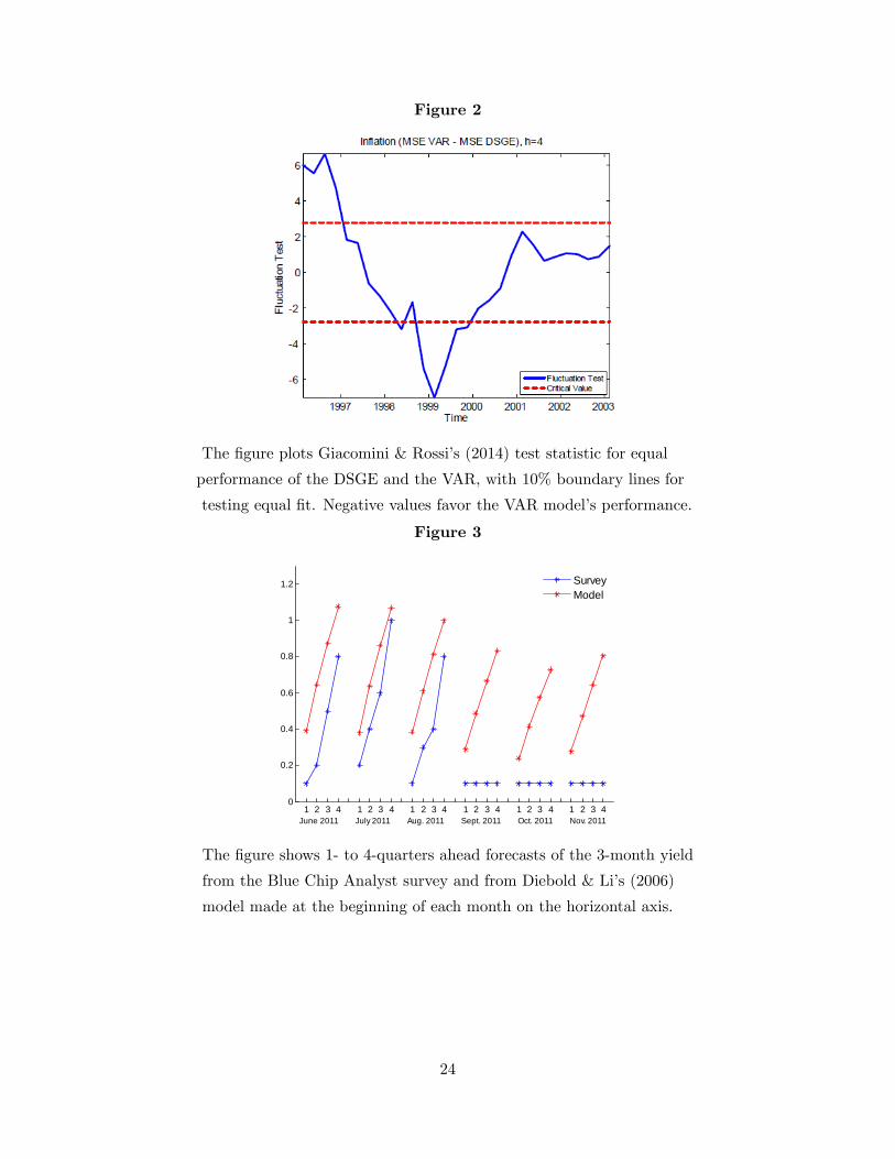
Figure 2
The �gure plots Giacomini & Rossi�s (2014) test statistic for equal
performance of the DSGE and the VAR, with 10% boundary lines for
testing equal �t. Negative values favor the VAR model�s performance.
Figure 3
1 2 3 4 1 2 3 4 1 2 3 4 1 2 3 4 1 2 3 4 1 2 3 40
0.2
0.4
0.6
0.8
1
1.2
June 2011 July 2011 Aug. 2011 Sept. 2011 Oct. 2011 Nov. 2011
SurveyModel
The �gure shows 1- to 4-quarters ahead forecasts of the 3-month yield
from the Blue Chip Analyst survey and from Diebold & Li�s (2006)
model made at the beginning of each month on the horizontal axis.
24

Table 1. Critical values (k�;�)
�
� 0.05 0.10
10% 3.176 2.928
20% 2.938 2.676
30% 2.770 2.482
40% 2.624 2.334
50% 2.475 2.168
60% 2.352 2.030
70% 2.248 1.904
80% 2.080 1.740
90% 1.975 1.600
Notes. The table shows the critical value for the informational e¢ ciency test described in Section 2.
25

References
Adolfson M, Linde J, Villani M. 2007. Forecasting performance of an open economy Dynamic
Stochastic General Equilibrium model. Econometric Reviews 26: 289�328.
Altavilla C, Giacomini R, Ragusa G. 2013. Anchoring the yield curve using survey expectations.
Centre for Microdata Methods and Practice. CeMMAP Working Paper 52/13. London: The
Institute for Fiscal Studies.
Amisano G, Giacomini R. 2007. Comparing density forecasts via weighted Likelihood ratio
tests. Journal of Business and Economic Statistics 25(2): 177�190.
Andrade P, Ghysels E, Idier J. 2012. Tails of in�ation forecasts and tales of monetary policy.
Banque of France Working Paper 407. Paris: Banque of France.
Andrews DWK. 1993. Tests for parameter instability and atructural change with unknown
xhange point. Econometrica 61(4): 821�856.
Andrews DWK, Ploberger W. 1994. Optimal tests when a nuisance parameter is present only
under the alternative. Econometrica 62(6): 1383�1414.
Bai J, Ng S. 2002. Determining the number of factors in approximate factor models. Econo-
metrica 70(1): 191�221.
Bai J, Perron P. 1998. Estimating and testing linear models with multiple structural changes.
Econometrica 66: 47�78.
Banbura M, Giannone D, Reichlin L. 2010. Large Bayesian vector auto regressions. Journal of
Applied Econometrics 25: 71�92.
Banerjee A, Marcellino M, Masten I. 2008. Forecasting macroeconomic variables using di¤usion
indexes in short samples with structural change. In: Forecasting in the Presence of Structural Breaks
and Model Uncertainty (Frontiers of Economics and Globalization), Vol. 3, ed. DE Rapach, ME
Wohar, pp. 149�194. Bingley (UK): Emerald Group Publishing Limited.
Bates B, Plagborg-Moller M, Stock J, Watson MW. 2013. Consistent factor estimation in
dynamic factor models with structural instability. Journal of Econometrics 177: 289�304.
Berkowitz, J. 2001. Testing density forecasts, with applications to risk management. Journal
of Business and Economic Statistics 19(4): 465�474.
Bianchi, F. 2013. Regime switches, agents�beliefs, and post-World War II U.S. macroeconomic
dynamics. Review of Economic Studies 80(2): 463�490.
Billio M, Casarin R, Ravazzolo F, Van Dijk H. 2013. Time-varying combinations of predictive
densities using nonlinear �ltering. Journal of Econometrics 177(2): 153�170.
Breitung J, Eickmeier S. 2011. Testing for structural breaks in dynamic factor models. Journal
of Econometrics 163(1): 71�84.
26

Brown R, Durbin J, Evans J. 1975. Techniques for testing the constancy of regression relation-
ships over time. Journal of the Royal Statistical Society Series B 37: 149�163.
Canova, F. 2006. Monetary policy and the evolution of the U.S. economy. Centre for Economics
Policy Research Working Paper 5467. London: CEPR.
Canova F, Ferroni F. 2011. Multiple �ltering devices for the estimation of cyclical DSGE models.
Journal of Quantitative Economics 2: 73�98.
Carriero A, Clark T, Marcellino M. 2011. Bayesian VARs: speci�cation choices and forecast
accuracy. FRB of Cleveland Working Paper 11�12. Cleveland (OH): Federal Reserve Bank of
Cleveland.
Chauvet M, Potter S. 2012. Forecasting output. In Handbook of Economic Forecasting, Vol. 2,
ed. G Elliott, A Timmermann, pp. 1�56. Amsterdam: Elsevier-North Holland.
Chun, A. 2008. Forecasting interest rates and in�ation: Blue Chip clairvoyants or econometrics?
Mimeo.
Clarida R, Galí J, Gertler M. 2000. Monetary policy rules and macroeconomic stability: evi-
dence and some theory. The Quarterly Journal of Economics 115(1): 147�180.
Clark, TE. 2011. Real-time density forecasts from Bayesian vector autoregressions with sto-
chastic volatility. Journal of Business and Economic Statistics 29(3): 327�341.
Cogley T, Sargent TJ. 2005. Drifts and volatilities: monetary policies and outcomes in the post
WWII U.S. Review of Economic Dynamics 8(2): 262�302.
Cogley T, Sbordone A. 2006. Trend in�ation and in�ation persistence in the new Keynesian
Phillips curve. FRB of New York Sta¤ Report 270. New York: Federal Reserve Bank of New York.
Coibion O, Gorodnichenko Y. 2012. What can survey forecasts tell us about informational
rigidities? Journal of Political Economy 120: 116�159.
Corradi V, Swanson NR. 2006. Predictive density evaluation. In Handbook of Economic Fore-
casting, Vol. 1, ed. G Elliott, CWJ Granger, A Timmermann, pp. 197�284. Amsterdam: Elsevier-
North Holland.
D�Agostino A, Gambetti L, Giannone D. 2013. Macroeconomic forecasting and structural
change. Journal of Applied Econometrics 28(1): 82-101.
Davig T, Leeper EM. 2007. Generalizing the Taylor principle. American Economic Review 97:
607�635.
De Mol C, Giannone D, Reichlin L. 2008. Forecasting using a large number of predictors: is
Bayesian shrinkage a valid alternative to principal components? Journal of Econometrics 146:
318�328.
Del Negro M, Schorfheide F. 2012. DSGE model-based forecasting. Federal Reserve Bank of
New York Sta¤ Report 554. New York: Federal Reserve Bank of New York.
Del Negro M, Giannoni M, chorfheide F. 2013. In�ation in the Great Recession and New
27

Keynesian models. Federal Reserve Bank of New York Sta¤ Report 618. New York: Federal
Reserve Bank of New York.
Diebold FX, Gunther TA, Tay AS. 1998. Evaluating density forecasts with applications to
�nancial risk management. International Economic Review 39(4): 863�883.
Diebold FX, Li C. 2006. Forecasting the term structure of government bond yields. Journal of
Econometrics 130: 337�364.
Diebold FX, Tay AS, Wallis KF. 1999. Evaluating density forecasts of in�ation: the survey of
professional forecasters. In Cointegration, Causality, and Forecasting: A Festschrift in Honour of
Clive W.J. Granger, ed. RF Engle, H White H, pp. 76�90. Oxford: Oxford University Press.
Diks C, Panchenko V, Van Dijk D. 2011. Likelihood-based scoring rules for comparing density
forecasts in tails. Journal of Econometrics 163(2): 215�230.
Edge RM, Gürkaynak RS. 2010. How useful are estimated DSGE model forecasts for central
bankers? Brookings Papers on Economic Activity 41: 209�259.
Eickmeier S, Lemke W, Marcellino M. 2011. Classical time-varying FAVARmodels - Estimation,
forecasting and structural analysis. Deutsche Bundesbank Discussion Paper 04-2011. Frankfurt:
Deutsche Bundesbank.
Elliott G, Müller U. 2006. E¢ cient tests for general persistent time variation in regression
coe¢ cients. Review of Economic Studies 73: 907�940.
Farmer R, Waggoner D, Zha T. 2009. Indeterminacy in a forward looking regime switching
model. International Journal of Economic Theory 5: 69�84.
Faust J, Wright JH. 2013. Forecasting in�ation. In Handbook of Economic Forecasting, Vol. 2,
ed. G Elliott, A Timmermann, pp. 3-56. Amsterdam: Elsevier-North Holland.
Fernández-Villaverde J, Rubio-Ramírez JF. 2008. How structural are structural parameters?
In NBER Macroeconomics Annual 2007, Vol. 22, ed. D Acemoglu, K Rogo¤, M Woodford, pp.
83�137. Chicago: University of Chicago Press.
Foerster A, Rubio-Ramirez J, Waggoner D, Zha T. 2013. Perturbation methods for Markov-
switching DSGE model. Federal Reserve Bank of Kansas City Research Working Paper 13-01.
Kansas City (Mo.): Federal Reserve Bank of Kansas City.
Forni M, Hallin M, Lippi M, Reichlin L. 2000. The generalized dynamic-factor model: Identi-
�cation and estimation. Review of Economics and Statistics 82(4): 540�554.
Giacomini, R. 2014. Economic theory and forecasting: lessons from the literature. Mimeo.
Giacomini R, Ragusa G. 2014. Theory-coherent forecasting. Journal of Econometrics 182:
145�155.
Giacomini R, Rossi B. 2009. Detecting and predicting forecast breakdown. Review of Economic
Studies 76(2): 669�705.
Giacomini R, Rossi B. 2010. Forecast comparisons in unstable environments. Journal of Applied
28

Econometrics 25(4): 595�620.
Giacomini R, Rossi B. 2014. Model comparisons in unstable environments. Barcelona Graduate
School of Economics Working Paper 784. Barcelona: Barcelona GSE.
Giacomini R, Rossi B. 2006. How stable is the forecasting performance of the yield curve for
output growth? Oxford Bulletin of Economics and Statistics 68(s1): 783-795.
Giannone D, Lenza M, Primiceri G. 2012. Prior selection for Vector Autoregressions. Review
of Economics and Statistics, In press.
Giraitis L, Kapetanios G, Price S. 2013. Adaptive forecasting in the presence of recent and
ongoing structural change. Journal of Econometrics 177(2): 153�170.
Groen JJJ, Paap R, Ravazzolo F. 2013. Real-time in�ation forecasting in a changing world.
Journal of Business and Economic Statistics 31(1): 29�44.
Gurkaynak R, K¬sac¬ko¼glu B, Rossi B. 2013. Do DSGE models forecast more accurately out-of-
sample than reduced-form models?. In VAR Models in Macroeconomics, Financial Econometrics,
and Forecasting - New Developments and Applications Essays in Honor of Christopher A. Sims,
Advances in Econometrics, Vol. 32, ed. T Fomby, L Kilian, A Murphy, pp. 27�80. Bingley UK:
Emerald Insight.
Hurwicz, L. 1962. On the structural form of interdependent systems. In Methodology and
Philosophy of Science. Proceedings of the 1960 International Congress, ed. L. Nagel, P Suppes, A
Tarski, pp. 232�239. Stanford (CA): Stanford University Press.
Ilut C, Schneider M. 2012. Ambiguous business cycles. National Bureau of Economic Research
Working Paper 17900. Cambridge (MA): NBER.
Inoue A. 2001. Testing for distributional change in time series. Econometric Theory 17(1):
156�187.
Inoue A, Kuo CH, Rossi B. 2014. Identifying the sources of model misspeci�cation. Centre for
Economic Policy Research Working Paper 10140. London: CEPR.
Inoue A, Rossi B. 2012. Out-of-sample forecast tests robust to the choice of window size.
Journal of Business and Economic Statistics 30(3): 432�453.
Inoue A, Rossi B. 2011. Identifying the sources of instabilities in macroeconomic �uctuations.
The Review of Economics and Statistics 93(4): 1186�1204.
Jore AS, Mitchell J, Vahey SP. 2010. Combining forecast densities from VARs with uncertain
instabilities. Journal of Applied Econometrics 25(4): 621�634.
Justiniano A, Primiceri G. 2008. The time-varying volatility of macroeconomic �uctuations.
American Economic Review 98: 604�41.
Kim, CJ, Nelson CR. 1999. Has the U.S. economy become more stable? A Bayesian approach
based on a Markov-switching model of the business cycle. Review of Economics and Statistics
81(4): 608�616.
29

Koop, G. 2013. Forecasting with medium and large Bayesian VARs. Journal of Applied Econo-
metrics 28(2): 177�203.
Koop G, Korobilis D. 2013. Large time-varying parameter VARs. Journal of Econometrics
177(2): 185�198.
Korobilis D, 2013. Assessing the transmission of monetary policy using time-varying parameter
dynamic factor models. Oxford Bulletin of Economics and Statistics 75(2): 157�179.
Manzan S, Zerom D. 2013. Are macroeconomic variables useful for forecasting the distribution
of U.S. in�ation? International Journal of Forecasting 29(3): 469�478.
McConnell MM, Pérez-Quirós G. 2000. Output �uctuations in the United States: What has
changed since the early 1980�s? American Economic Review 90(5): 1464�1476.
Mitchell J, Wallis KF. 2011. Evaluating density forecasts: Forecast combinations, model mix-
tures, calibration and sharpness. Journal of Applied Econometrics 26(6): 1023�1040.
Monti F. 2010. Combining judgment and models. Journal of Money, Credit and Banking 42:
1641-1662.
Müller U, Petalas PE. 2010. E¢ cient estimation of the parameter path in unstable time series
models. Review of Economic Studies 77: 1508�1539.
Ng S, Wright JH. 2013. Facts and challenges from the Great Recession for forecasting and
macroeconomic modeling. Journal of Economic Literature 51(4): 1120�1154.
Nyblom, J. 1989. Testing for the constancy of parameters over time. Journal of the American
Statistical Association 84: 223�230.
Pesaran MH, Pettenuzzo D, Timmermann A. 2006. Forecasting time series subject to multiple
structural breaks. The Review of Economic Studies 73(4): 1057�1084.
Pesaran MH, Pick A, Pranovich M. 2013. Optimal forecasts in the presence of structural breaks.
Journal of Econometrics 177(2): 134�152.
Pesaran MH, Timmermann A. 2007. Selection of estimation window in the presence of breaks.
Journal of Econometrics 137: 134�161.
Pesaran MH, Timmermann A. 2002. Market timing and return prediction under model insta-
bility. Journal of Empirical Finance 9(5): 495�510.
Ploberger W, Krämer W. 1992. The CUSUM Test with OLS residuals. Econometrica 60:
271�285.
Ploberger W, Krämer W, Kontrus K. 1989. A new test for structural stability in the linear
regression model. Journal of Econometrics 40: 307�318.
Primiceri G. 2005. Time varying structural Vector Autoregressions and monetary policy. Review
of Economic Studies 72(3): 821�852.
Robertson JC, Tallman EW, Whiteman CH. 2005. Forecasting using relative entropy. Journal
of Money, Credit and Banking 37: 383�401.
30

Rossi, B. 2013. Advances in forecasting under instabilities. In Handbook of Economic Forecast-
ing, Vol. 2, ed. G Elliott, A Timmermann, pp. 1203-1324. Amsterdam: Elsevier-North Holland.
Rossi B, Sekhposyan T. 2014. Evaluating predictive densities of US output growth and in�ation
in a large macroeconomic data set. International Journal of Forecasting 30(3): 662�682.
Rossi B, Sekhposyan T. 2014. Forecast rationality tests in the presence of instabilities, with
applications to Federal Reserve and survey forecasts. Journal of Applied Econometrics: In press.
Rossi B, Sekhposyan. 2013. Conditional predictive density evaluation in the presence of insta-
bilities. Journal of Econometrics 177(2): 199�212.
Rossi B, Sekhposyan T. 2010. Have economic models�forecasting performance for US output
growth and in�ation changed over time, and when? International Journal of Forecasting 26(4):
808�835.
Sims, C. 2003. Comment on Smets and Wouters. Princeton University. https://sims.princeton.edu/
yftp/Ottawa/SWcommentSlides.pdf
Sims C, Zha T. 2006. Were there regime switches in U.S. monetary policy? American Economic
Review 96(1): 54�81.
Smets F, Wouters R. 2007. Shocks and frictions in US business cycles: A Bayesian DSGE
approach. American Economic Review 97: 586�606.
Stock JH, Watson MW. 1996. Evidence on structural instability in macroeconomic time series
relations. Journal of Business and Economic Statistics 14(1): 11�30.
Stock JH, Watson MW. 2002. Forecasting using principal components from a large number of
predictors. Journal of the American Statistical Association 97(460): 1167�1179.
Stock JH, Watson MW. 2003. Has the business cycle changed and why? In NBER Macroeco-
nomics Annual 2002, Vol. 17, ed. M Gertler, K Rogo¤, pp. 159�230. Cambridge (MA): National
Bureau of Economic Research.
Stock JH, Watson MW. 2003. Forecasting output and in�ation: The role of asset prices. Journal
of Economic Literature 41(3): 788�829.
Stock JH, Watson MW. 2004. Combination forecasts of output growth in a seven country data
set. Journal of Forecasting 23(6): 405�430.
Stock JH, Watson MW. 2006. Forecasting with many predictors. In Handbook of Economic
Forecasting, Vol. 1, ed. G Elliott, CWJ Granger, A Timmermann, pp. 515�554. Amsterdam:
Elsevier-North Holland.
Stock JH, Watson MW. 2007. Has in�ation become harder to forecast? Journal of Money,
Credit and Banking 39(1): 3�33.
Stock JH, Watson MW. 2009. Forecasting in dynamic factor models subject to structural
instability. In The Methodology and Practice of Econometrics: A Festschrift in Honour of David
F. Hendry, ed. DF Hendry, J Castle, N Shephard, pp. 173�205. Oxford: Oxford University Press.
31

Timmermann A. 2006. Forecast combinations. In Handbook of Economic Forecasting, Vol. 1,
ed. G Elliott, CWJ Granger, A Timmermann, pp. 135�196. Amsterdam: Elsevier-North Holland.
Wieland V, Cwik T, Müller GJ, Schmidt S, Wolters MH. 2012. A new comparative approach
to macroeconomic modelling and policy analysis. Center for Financial Studies. Mimeo. Frankfurt:
CFS.
Wright, JH. 2009. Forecasting US in�ation by Bayesian model averaging. Journal of Forecasting
28(2): 131�144.
Wolden Bache I, So�e Jore A, Mitchell J, Vahey SP. 2011. Combining VAR and DSGE forecast
densities. Journal of Economic Dynamics and Control 35(10): 1659-1670.
32
Recommended