Graduate Theses and Dissertations Iowa State University Capstones, Theses andDissertations
2011
Floorplan-guided placement for large-scale mixed-size designsZijun YanIowa State University
Follow this and additional works at: https://lib.dr.iastate.edu/etd
Part of the Electrical and Computer Engineering Commons
This Dissertation is brought to you for free and open access by the Iowa State University Capstones, Theses and Dissertations at Iowa State UniversityDigital Repository. It has been accepted for inclusion in Graduate Theses and Dissertations by an authorized administrator of Iowa State UniversityDigital Repository. For more information, please contact [email protected].
Recommended CitationYan, Zijun, "Floorplan-guided placement for large-scale mixed-size designs" (2011). Graduate Theses and Dissertations. 12209.https://lib.dr.iastate.edu/etd/12209

Floorplan-guided placement for large-scale mixed-size designs
by
Zijun Yan
A dissertation submitted to the graduate faculty
in partial fulfillment of the requirements for the degree of
DOCTOR OF PHILOSOPHY
Major: Computer Engineering
Program of Study Committee:Chris C.-N. Chu, Major Professor
Randall L. GeigerSigurdur Olafsson
Akhilesh TyagiJoseph A. Zambreno
Iowa State University
Ames, Iowa
2011
Copyright c© Zijun Yan, 2011. All rights reserved.

ii
To my mom Shuxian Min,
and to the memory of
my uncle Dabao Min and my grandma Namei Li
. . .
(all is beyond words)
iii
TABLE OF CONTENTS
LIST OF TABLES . . . . . . . . . . . . . . . . . . . . . . . . . . . . . . . . . . . . . . . . . vii
LIST OF FIGURES . . . . . . . . . . . . . . . . . . . . . . . . . . . . . . . . . . . . . . . . ix
ACKNOWLEDGMENTS . . . . . . . . . . . . . . . . . . . . . . . . . . . . . . . . . . . . . xi
ABSTRACT . . . . . . . . . . . . . . . . . . . . . . . . . . . . . . . . . . . . . . . . . . . . xiii
CHAPTER 1 Introduction . . . . . . . . . . . . . . . . . . . . . . . . . . . . . . . . . . . 1
1.1 Modern Mixed-Size Placement . . . . . . . . . . . . . . . . . . . . . . . . . . . . . . 1
1.2 Previous Work . . . . . . . . . . . . . . . . . . . . . . . . . . . . . . . . . . . . . . . 2
1.3 New Algorithm Flow and Key Techniques . . . . . . . . . . . . . . . . . . . . . . . . 3
1.4 Dissertation Organization . . . . . . . . . . . . . . . . . . . . . . . . . . . . . . . . . 6
Note About Bibliography . . . . . . . . . . . . . . . . . . . . . . . . . . . . . . . . . . . . 6
CHAPTER 2 Fixed-Outline Floorplanning . . . . . . . . . . . . . . . . . . . . . . . . . . 8
2.1 Introduction . . . . . . . . . . . . . . . . . . . . . . . . . . . . . . . . . . . . . . . . 8
2.1.1 Previous Work . . . . . . . . . . . . . . . . . . . . . . . . . . . . . . . . . . 8
2.1.2 Our Contributions . . . . . . . . . . . . . . . . . . . . . . . . . . . . . . . . 10
2.2 Algorithm Flow of DeFer . . . . . . . . . . . . . . . . . . . . . . . . . . . . . . . . . 12
2.3 Generalized Slicing Tree . . . . . . . . . . . . . . . . . . . . . . . . . . . . . . . . . 15
2.3.1 Notion of Generalized Slicing Tree . . . . . . . . . . . . . . . . . . . . . . . 15
2.3.2 Extended Shape Curve Operation . . . . . . . . . . . . . . . . . . . . . . . . 16
2.3.3 Decision of Slice Line Direction for Terminal Propagation . . . . . . . . . . . 17
2.4 Whitespace-Aware Pruning . . . . . . . . . . . . . . . . . . . . . . . . . . . . . . . . 17
2.4.1 Motivation on WAP . . . . . . . . . . . . . . . . . . . . . . . . . . . . . . . . 17
iv
2.4.2 Problem Formulation of WAP . . . . . . . . . . . . . . . . . . . . . . . . . . 18
2.4.3 Solving WAP . . . . . . . . . . . . . . . . . . . . . . . . . . . . . . . . . . . 21
2.5 Enumerative Packing . . . . . . . . . . . . . . . . . . . . . . . . . . . . . . . . . . . 22
2.5.1 A Naive Approach of Enumeration . . . . . . . . . . . . . . . . . . . . . . . 22
2.5.2 Enumeration by Dynamic Programming . . . . . . . . . . . . . . . . . . . . . 23
2.5.3 Impact of EP on Packing . . . . . . . . . . . . . . . . . . . . . . . . . . . . . 24
2.5.4 High-Level EP . . . . . . . . . . . . . . . . . . . . . . . . . . . . . . . . . . 25
2.6 Block Swapping and Mirroring . . . . . . . . . . . . . . . . . . . . . . . . . . . . . . 27
2.7 Extension of DeFer . . . . . . . . . . . . . . . . . . . . . . . . . . . . . . . . . . . . 28
2.8 Implementation Details . . . . . . . . . . . . . . . . . . . . . . . . . . . . . . . . . . 30
2.9 Experimental Results . . . . . . . . . . . . . . . . . . . . . . . . . . . . . . . . . . . 32
2.9.1 Experiments on Fixed-Outline Floorplanning . . . . . . . . . . . . . . . . . . 32
2.9.2 Experiments on Classical Outline-Free Floorplanning . . . . . . . . . . . . . . 44
2.10 Conclusion . . . . . . . . . . . . . . . . . . . . . . . . . . . . . . . . . . . . . . . . 46
CHAPTER 3 General Floorplan-Guided Placement . . . . . . . . . . . . . . . . . . . . . 47
3.1 Introduction . . . . . . . . . . . . . . . . . . . . . . . . . . . . . . . . . . . . . . . . 47
3.2 Overview of FLOP . . . . . . . . . . . . . . . . . . . . . . . . . . . . . . . . . . . . 47
3.3 Block Formation and Floorplanning . . . . . . . . . . . . . . . . . . . . . . . . . . . 48
3.3.1 Usage of Exact Net Model . . . . . . . . . . . . . . . . . . . . . . . . . . . . 49
3.3.2 Block Formation . . . . . . . . . . . . . . . . . . . . . . . . . . . . . . . . . 50
3.3.3 Generation of Shape Curve for Blocks . . . . . . . . . . . . . . . . . . . . . . 51
3.4 Wirelength-Driven Shifting . . . . . . . . . . . . . . . . . . . . . . . . . . . . . . . . 51
3.5 Incremental Placement . . . . . . . . . . . . . . . . . . . . . . . . . . . . . . . . . . 52
3.6 MMS Benchmarks . . . . . . . . . . . . . . . . . . . . . . . . . . . . . . . . . . . . 52
3.7 Experimental Results . . . . . . . . . . . . . . . . . . . . . . . . . . . . . . . . . . . 57
3.8 Conclusion . . . . . . . . . . . . . . . . . . . . . . . . . . . . . . . . . . . . . . . . 61
CHAPTER 4 Hypergraph Clustering for Wirelength-Driven Placement . . . . . . . . . . 62
4.1 Introduction . . . . . . . . . . . . . . . . . . . . . . . . . . . . . . . . . . . . . . . . 62

v
4.1.1 Previous Work . . . . . . . . . . . . . . . . . . . . . . . . . . . . . . . . . . 62
4.1.2 Our Contributions . . . . . . . . . . . . . . . . . . . . . . . . . . . . . . . . 64
4.2 Safe Clustering . . . . . . . . . . . . . . . . . . . . . . . . . . . . . . . . . . . . . . 66
4.2.1 Concept of Safe Clustering . . . . . . . . . . . . . . . . . . . . . . . . . . . . 66
4.2.2 Safe Condition for Pair-Wise Clustering . . . . . . . . . . . . . . . . . . . . . 67
4.2.3 Selective Enumeration . . . . . . . . . . . . . . . . . . . . . . . . . . . . . . 69
4.3 Algorithm of SafeChoice . . . . . . . . . . . . . . . . . . . . . . . . . . . . . . . . . 76
4.3.1 Priority-Queue Based Framework . . . . . . . . . . . . . . . . . . . . . . . . 77
4.3.2 Operation Modes of SafeChoice . . . . . . . . . . . . . . . . . . . . . . . . . 77
4.4 Physical SafeChoice . . . . . . . . . . . . . . . . . . . . . . . . . . . . . . . . . . . . 79
4.4.1 Safe Condition for Physical SafeChoice . . . . . . . . . . . . . . . . . . . . . 79
4.4.2 Enumeration Size Reduction based on Physical Location . . . . . . . . . . . . 80
4.4.3 Cost Function for Physical SafeChoice . . . . . . . . . . . . . . . . . . . . . . 81
4.5 SafeChoice-Based Two-Phase Placement . . . . . . . . . . . . . . . . . . . . . . . . 81
4.6 Experimental Results . . . . . . . . . . . . . . . . . . . . . . . . . . . . . . . . . . . 83
4.6.1 Comparison of Clustering Algorithms . . . . . . . . . . . . . . . . . . . . . . 84
4.6.2 Comparison of Placement Algorithms . . . . . . . . . . . . . . . . . . . . . . 96
4.7 Conclusion . . . . . . . . . . . . . . . . . . . . . . . . . . . . . . . . . . . . . . . . 99
CHAPTER 5 Soft-Block Shaping in Floorplanning . . . . . . . . . . . . . . . . . . . . . . 100
5.1 Introduction . . . . . . . . . . . . . . . . . . . . . . . . . . . . . . . . . . . . . . . . 100
5.1.1 Previous Work . . . . . . . . . . . . . . . . . . . . . . . . . . . . . . . . . . 100
5.1.2 Our Contributions . . . . . . . . . . . . . . . . . . . . . . . . . . . . . . . . 101
5.2 Problem Formulation . . . . . . . . . . . . . . . . . . . . . . . . . . . . . . . . . . . 103
5.3 Basic Slack-Driven Shaping . . . . . . . . . . . . . . . . . . . . . . . . . . . . . . . 104
5.3.1 Target Soft Blocks . . . . . . . . . . . . . . . . . . . . . . . . . . . . . . . . 106
5.3.2 Shaping Scheme . . . . . . . . . . . . . . . . . . . . . . . . . . . . . . . . . 107
5.3.3 Flow of Basic Slack-Driven Shaping . . . . . . . . . . . . . . . . . . . . . . . 109
5.4 Optimality Conditions . . . . . . . . . . . . . . . . . . . . . . . . . . . . . . . . . . 111
vi
5.5 Flow of Slack-Driven Shaping . . . . . . . . . . . . . . . . . . . . . . . . . . . . . . 113
5.6 Experimental Results . . . . . . . . . . . . . . . . . . . . . . . . . . . . . . . . . . . 115
5.6.1 Experiments on MCNC Benchmarks . . . . . . . . . . . . . . . . . . . . . . . 116
5.6.2 Experiments on HB Benchmarks . . . . . . . . . . . . . . . . . . . . . . . . . 118
5.7 Conclusion . . . . . . . . . . . . . . . . . . . . . . . . . . . . . . . . . . . . . . . . 122
CHAPTER 6 Geometry Constraint Aware Floorplan-Guided Placement . . . . . . . . . 123
6.1 Introduction . . . . . . . . . . . . . . . . . . . . . . . . . . . . . . . . . . . . . . . . 123
6.2 Overview of FLOPC . . . . . . . . . . . . . . . . . . . . . . . . . . . . . . . . . . . 123
6.3 Enhanced Annealing-Based Floorplanning . . . . . . . . . . . . . . . . . . . . . . . . 124
6.3.1 Sequence Pair Generation from Given Layout . . . . . . . . . . . . . . . . . . 125
6.3.2 Sequence Pair Insertion with Location Awareness . . . . . . . . . . . . . . . . 129
6.3.3 Constraint Handling and Annealing Schedule . . . . . . . . . . . . . . . . . . 131
6.4 Experimental Results . . . . . . . . . . . . . . . . . . . . . . . . . . . . . . . . . . . 132
6.5 Conclusion . . . . . . . . . . . . . . . . . . . . . . . . . . . . . . . . . . . . . . . . 133
BIBLIOGRAPHY . . . . . . . . . . . . . . . . . . . . . . . . . . . . . . . . . . . . . . . . . 136
vii
LIST OF TABLES
Table 2.1 Comparison on # of ‘⊕’ operation. . . . . . . . . . . . . . . . . . . . . . . . 24
Table 2.2 Comparison on GSRC Hard-Block benchmarks. . . . . . . . . . . . . . . . . 35
Table 2.3 Comparison on GSRC Soft-Block benchmarks. . . . . . . . . . . . . . . . . 37
Table 2.4 Comparison on HB benchmarks. . . . . . . . . . . . . . . . . . . . . . . . . 40
Table 2.5 Comparison on HB+ benchmarks. . . . . . . . . . . . . . . . . . . . . . . . 43
Table 2.6 Comparison on linear combination of HPWL and area. . . . . . . . . . . . . 45
Table 2.7 Contributions of main techniques and runtime breakdown in DeFer. . . . . . 45
Table 3.1 Statistics of Modern Mixed-Size placement benchmarks. . . . . . . . . . . . 55
Table 3.2 Comparison with mixed-size placers on MMS benchmarks. . . . . . . . . . . 59
Table 3.3 Comparison with macro placers on modified ISPD06 benchmarks. . . . . . . 60
Table 4.1 Profile of selective enumeration for each circuit. . . . . . . . . . . . . . . . . 76
Table 4.2 Differences of three modes in SafeChoice. . . . . . . . . . . . . . . . . . . . 78
Table 4.3 S∗ for three modes in Physical SafeChoice. . . . . . . . . . . . . . . . . . . 81
Table 4.4 Comparison with FirstChoice and BestChoice. . . . . . . . . . . . . . . . . . 86
Table 4.5 Comparison with FirstChoice, BestChoice and NetCluster. . . . . . . . . . . 88
Table 4.6 Comparison with FirstChoice and BestChoice on various target γ. . . . . . . 90
Table 4.7 Comparison with multilevel mPL6. . . . . . . . . . . . . . . . . . . . . . . . 95
Table 4.8 Comparison with original multilevel mPL6. . . . . . . . . . . . . . . . . . . 96
Table 4.9 HPWL comparison with state-of-the-art placement algorithms. . . . . . . . . 98
Table 4.10 Runtime breakdown of SCPlace. . . . . . . . . . . . . . . . . . . . . . . . . 99
Table 5.1 Comparison with Young et al.’s algorithm on MCNC benchmarks. . . . . . . 117

viii
Table 5.2 Comparison with Lin et al.’s algorithm on MCNC benchmarks. . . . . . . . . 117
Table 5.3 Comparison on runtime complexity. . . . . . . . . . . . . . . . . . . . . . . 118
Table 5.4 Experimental results of SDS on HB benchmarks. . . . . . . . . . . . . . . . 120
Table 6.1 List of geometry constraints in MMS benchmarks. . . . . . . . . . . . . . . . 133
Table 6.2 Comparison with mixed-size placers on MMS benchmarks with constraints. . 134
ix
LIST OF FIGURES
Figure 1.1 Example of modern mixed-size circuit. . . . . . . . . . . . . . . . . . . . . . 2
Figure 1.2 Previous two-stage approach to handle mixed-size designs. . . . . . . . . . . 3
Figure 1.3 New algorithm flow for mixed-size placement. . . . . . . . . . . . . . . . . . 4
Figure 2.1 Pseudocode on algorithm flow of DeFer. . . . . . . . . . . . . . . . . . . . . 12
Figure 2.2 High-level slicing tree. . . . . . . . . . . . . . . . . . . . . . . . . . . . . . 13
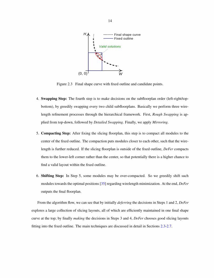
Figure 2.3 Final shape curve with fixed outline and candidate points. . . . . . . . . . . . 14
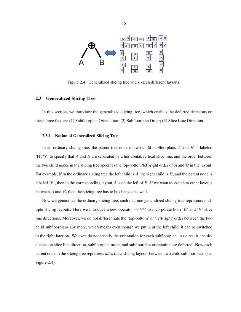
Figure 2.4 Generalized slicing tree and sixteen different layouts. . . . . . . . . . . . . . 15
Figure 2.5 Extended shape curve operation. . . . . . . . . . . . . . . . . . . . . . . . . 16
Figure 2.6 Generation of whitespace during curve combination. . . . . . . . . . . . . . 18
Figure 2.7 Calculation of Wpi and Wo. . . . . . . . . . . . . . . . . . . . . . . . . . . . 20
Figure 2.8 List of different slicing tree structures. . . . . . . . . . . . . . . . . . . . . . 23
Figure 2.9 Illustration of high-level EP. . . . . . . . . . . . . . . . . . . . . . . . . . . 26
Figure 2.10 One exception of identifying hTree. . . . . . . . . . . . . . . . . . . . . . . 27
Figure 2.11 Swapping and Mirroring. . . . . . . . . . . . . . . . . . . . . . . . . . . . . 28
Figure 2.12 Motivation on Rough Swapping. . . . . . . . . . . . . . . . . . . . . . . . . 28
Figure 2.13 Compacting invalid points into fixed outline. . . . . . . . . . . . . . . . . . . 29
Figure 2.14 Two strategies of identifying hRoot. . . . . . . . . . . . . . . . . . . . . . . 31
Figure 2.15 Tuned parameters at each run in DeFer. . . . . . . . . . . . . . . . . . . . . 31
Figure 2.16 Circuit n300 layouts generated by DeFer. . . . . . . . . . . . . . . . . . . . 34
Figure 2.17 Circuit ibm03 layouts generated by PATOMA, Capo 10.5 and DeFer. . . . . . 39
Figure 3.1 Generation of shape curves for blocks. . . . . . . . . . . . . . . . . . . . . . 51

x
Figure 3.2 Algorithm of analytical incremental placement. . . . . . . . . . . . . . . . . 53
Figure 3.3 Runtime breakdown of FLOP. . . . . . . . . . . . . . . . . . . . . . . . . . 58
Figure 4.1 Example of indirect connections between objects a and b. . . . . . . . . . . . 64
Figure 4.2 Simple examples of vertices that can be fixed. . . . . . . . . . . . . . . . . . 72
Figure 4.3 Flow of selective enumeration. . . . . . . . . . . . . . . . . . . . . . . . . . 75
Figure 4.4 Examples of three scenarios with square-shape region. . . . . . . . . . . . . 81
Figure 4.5 Simple two-phase placement flow in SCPlace. . . . . . . . . . . . . . . . . . 82
Figure 4.6 Experimental flow for clustering algorithm. . . . . . . . . . . . . . . . . . . 84
Figure 4.7 Average normalized clustering time to SC-R. . . . . . . . . . . . . . . . . . 93
Figure 4.8 Average normalized HPWL to flat-mPL6. . . . . . . . . . . . . . . . . . . . 94
Figure 4.9 Average normalized total time to flag-mPL6. . . . . . . . . . . . . . . . . . . 94
Figure 5.1 Flow of basic slack-driven shaping. . . . . . . . . . . . . . . . . . . . . . . . 110
Figure 5.2 Example of a non-optimal solution from basic SDS. . . . . . . . . . . . . . . 112
Figure 5.3 Examples of three optimal cases in L. . . . . . . . . . . . . . . . . . . . . . 113
Figure 5.4 Flow of slack-driven shaping. . . . . . . . . . . . . . . . . . . . . . . . . . . 114
Figure 5.5 Layout-height convergence graphs of four circuits. . . . . . . . . . . . . . . 121
Figure 6.1 Flow of enhanced annealing-based floorplanning. . . . . . . . . . . . . . . . 126
Figure 6.2 Divided eight chip regions around block b. . . . . . . . . . . . . . . . . . . . 127
Figure 6.3 Calculation of insertion range in S+c . . . . . . . . . . . . . . . . . . . . . . . 134
Figure 6.4 Calculation of insertion range in S−c . . . . . . . . . . . . . . . . . . . . . . . 135

xi
ACKNOWLEDGMENTS
I would like to take this opportunity to express my thanks to the people who helped me on every
aspect of conducting this research and supporting my daily study, work and life.
First of all, I would like to express my deepest thanks to my advisor, Prof. Chris Chu, not only
for his patient guidance and great support through this research as a mentor, but also for his sincere
personality as a friend. I am deeply impressed by his novel ideas and invaluable insight on VLSI
physical design, his dedication to work and research, and his passion and belief in God. His guidance
and ideas have been involved in every aspect of my research work, from research topic selection to
experimental results analysis, from algorithm design to code implementation, from paper organization
to paper revision, from slides preparation to conference presentation, etc. Prof. Chu always asks me to
aim higher. Without his endless encouragement and constructive criticisms, I would never achieve this
far. He also provided me ample opportunities to be exposed to both industrial and academic occasions,
e.g., Cadence Research Labs internship, IBM on-site visit, DAC summer school, IBM Ph.D. Fellowship
application, etc. It has been such a remarkable experience to work with him, as my advisor. Besides
that, Chris is also a truly friend to talk with. For so many times, we have had deep discussions on
various topics including human life, Christianity, courtesy and politeness, correct attitude on personal
achievement and public recognition, career goals, various hobbies (e.g., fishing and physical exercises)
and so on. Both my professional and personal life have immensely benefited from these discussions.
Thank you!
Secondly, I would like to thank Prof. Randall Geiger, Prof. Olafsson Sigurdur, Prof. Akhilesh Tyagi
and Prof. Joseph Zambreno for their time to serve in my Ph.D. committee and valuable comments on
my work. I especially thank Joe. It was a great time to work with him during my early graduate period.
He was a “life saver” in several occasions: 1) He helped me to fix a latex problem just a couple of

xii
minutes before one paper submission deadline; 2) He fixed one critical bug in my code, which I may
never be able to figure out by myself.
Thirdly, I am also grateful to the colleagues at other universities and industrial companies for their
sharp comments and kindly assistance on my research. They are, but not limited to, Prof. Wai-Kei Mak
and Prof. Ting-Chi Wang from National Tsing Hua University, Prof. Robert Dick and Prof. Igor Markov
from University of Michigan, Prof. Yao-Wen Chang from National Taiwan University, Prof. Evan-
geline Young from Chinese University of Hong Kong, Prof. Hai Zhou from Northwestern Univer-
sity, Prof. George Karypis from University of Minnesota, Dr. Charles Alpert, Dr. Gi-Joon Nam and
Dr. Natarajan Viswanathan from IBM Austin Research Labs, Dr. Philip Chong and Dr. Christian Szegedy
from Cadence Research Labs, Guojie Luo from University of California, Los Angeles, Logan Rakai
from University of Calgary. Special thanks goes to Natarajan. His work and effort on FastPlace3, the
analytical placement algorithm, play a critical role in my research work. I am also greatly appreciated
my colleagues at Cadence Design Systems, Dr. Chin-Chi Teng, Dr. Dennis Huang and Dr. Lu Sha for
their understanding and supporting me to finish up this dissertation, while I am a full-time employee.
Last but not least, I want to express my thanks to the fellow friends at Iowa State University, Wanyu
Ye, Jiang Lin, Song Sun, Bojian Xu, Song Lu, Jerry Cao, Yanheng Zhang, Yue Xu, Enlai Xu, Xin Zhao,
Willis Alexander, Brice Batemon, Genesis Lightbourne, Steve Luhmann, Ranran Fan, George Hatfield,
Mallory Parmerlee and many others. They made my life at Ames, my first stop in U.S., so wonderful
and memorable!
To each of the above person, I extend my deepest appreciation . . .
Sunnyvale, California
May 26, 2011

xiii
ABSTRACT
In the nanometer scale era, placement has become an extremely challenging stage in modern Very-
Large-Scale Integration (VLSI) designs. Millions of objects need to be placed legally within a chip
region, while both the interconnection and object distribution have to be optimized simultaneously. Due
to the extensive use of Intellectual Property (IP) and embedded memory blocks, a design usually con-
tains tens or even hundreds of big macros. A design with big movable macros and numerous standard
cells is known as mixed-size design. Due to the big size difference between big macros and standard
cells, the placement of mixed-size designs is much more difficult than the standard-cell placement.
This work 1 presents an efficient and high-quality placement tool to handle modern large-scale
mixed-size designs. This tool is developed based on a new placement algorithm flow. The main idea
is to use the fixed-outline floorplanning algorithm to guide the state-of-the-art analytical placer. This
new flow consists of four steps: 1) The objects in the original netlist are clustered into blocks; 2)
Floorplanning is performed on the blocks; 3) The blocks are shifted within the chip region to further
optimize the wirelength; 4) With big macro locations fixed, incremental placement is applied to place
the remaining objects. Several key techniques are proposed to be used in the first two steps. These
techniques are mainly focused on the following two aspects: 1) Hypergraph clustering algorithm that
can cut down the original problem size without loss of placement Quality of Results (QoR); 2) Fixed-
outline floorplanning algorithm that can provide a good guidance to the analytical placer at the global
level.
The effectiveness of each key technique is demonstrated by promising experimental results com-
pared with the state-of-the-art algorithms. Moreover, using the industrial mixed-size designs, the new
placement tool shows better performance than other existing approaches.
1This work was partially supported by IBM Faculty Award, NSF under grant CCF-0540998 and NSC under grant NSC99-2220-E-007-007.
1
CHAPTER 1 Introduction
A journey of a thousand miles starts with a single step and
if that step is the right step, it becomes the last step.
— Lao Tzu
1.1 Modern Mixed-Size Placement
In the nanometer scale era, placement has become an extremely challenging stage in modern VLSI
designs. Millions of objects need to be placed legally within a chip region, while both the intercon-
nection and object distribution have to be optimized simultaneously. As an early step of VLSI physical
design flow, the quality of the placement solution has significant impacts on both routing and manu-
facturing. In modern System-on-Chip (SoC) designs, the usage of IP and embedded memory blocks
becomes more and more popular. As a result, a design usually contains tens or even hundreds of big
macros which can be either movable or preplaced. A design with big macros and numerous standard
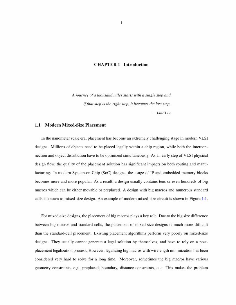
cells is known as mixed-size design. An example of modern mixed-size circuit is shown in Figure 1.1.
For mixed-size designs, the placement of big macros plays a key role. Due to the big size difference
between big macros and standard cells, the placement of mixed-size designs is much more difficult
than the standard-cell placement. Existing placement algorithms perform very poorly on mixed-size
designs. They usually cannot generate a legal solution by themselves, and have to rely on a post-
placement legalization process. However, legalizing big macros with wirelength minimization has been
considered very hard to solve for a long time. Moreover, sometimes the big macros have various
geometry constraints, e.g., preplaced, boundary, distance constraints, etc. This makes the problem
2
Figure 1.1 Example of modern mixed-size circuit, which contains 2177353 objects and 2228903 nets.The blue dots represent standard cells, and the white rectangular regions represent macros.
of mixed-size placement even harder. As existing placement algorithms simply cannot handle such
geometry constraints, the designer has to place these macros manually beforehand.
1.2 Previous Work
Most mixed-size placement algorithms place both the macros and the standard cells simultaneously.
Examples are the annealing-based placer Dragon [1], the partitioning-based placer Capo [2], and the
analytical placers FastPlace3 [3], APlace2 [4], Kraftwerk [5], mPL6 [6], and NTUplace3 [7]. The
analytical placers are the state-of-the-art placement algorithms. They can produce the best results in the
best runtime. However, the analytical approach has three problems. First, only an approximation (e.g.,
by log-sum-exp or quadratic function) of the HPWL is minimized. Second, the distribution of objects
is also approximated and that usually results in a substantial amount of overlaps. They have to rely on
a legalization step to resolve the overlaps. For mixed-size designs, such legalization process is very
difficult and is likely to significantly increase the wirelength. Third, analytical placers cannot optimize
macro orientations and handle various geometry constraints.
3
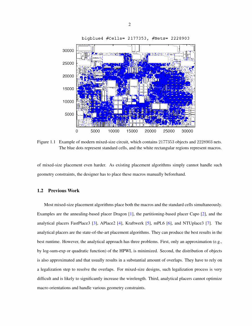
Macro Placer / Legalizer
Initial Placement
Standard-cell Placer
Stage 1 Stage 2
Figure 1.2 Previous two-stage approach to handle mixed-size designs.
Other researchers apply a two-stage approach as shown in Figure 1.2 to handle the mixed-size
placement. An initial wirelength-driven placement is first generated. Then a macro placement or legal-
ization algorithm is used to place only the macros, without considering the standard cells. After that,
the macros are fixed, and the standard cells are re-placed in the remaining whitespace from scratch.
As the macro placement is a crucial stage in this flow, people propose different techniques to improve
the QoR. Based on the MP-tree representation, Chen et al. [8] used a packing-based algorithm to place
the macros around the four corners of the chip region. In [9], a Transitive Closure Graph (TCG) based
technique was applied to enhance the quality of macro placement. One main problem with the above
two approaches is that the initial placement is produced with large amount of overlaps. Thus, the initial
solution may not provide good suggestions to the locations of objects. However, the following macro-
placement stage determines the macro locations by minimizing the displacement from the low-quality
initial placement.
Alternatively, Adya et al. [10] used an annealing-based floorplanner to directly minimize the HPWL
among the macros and clustered standard cells at the macro-placement stage. But, they still have to rely
on the illegal placement to determine the initial locations of macros and clusters. For all of the above
two-stage approaches, after fixing the macros, the initial positions of standard cells have to be discarded
to reduce the overlaps.
1.3 New Algorithm Flow and Key Techniques
In this dissertation, an efficient and high-quality placement tool is presented to effectively handle
the complexities of modern large-scale mixed-size placement. Such tool is developed based on a new
placement flow that integrates floorplanning and incremental placement algorithms. The main idea
of this flow is to use the fixed-outline floorplanner to guide the state-of-the-art analytical placer. As

4
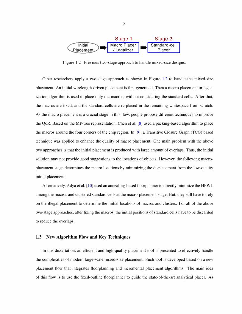
Block Formation
Wirelength-driven Shifting
Floorplanning
Incremental Placement
Figure 1.3 New algorithm flow for mixed-size placement.
floorplanners have a good capability of handling a small number of objects [2], we apply floorplan-
ning algorithm on the clustered circuit to generate a global overlap-free layout, and use it to guide the
subsequent placement algorithm.
The proposed new algorithm flow for mixed-size placement is as follows (see Figure 1.3).
1. Block Formation: The purpose of the first step is to cut down the problem size. We define
“small objects” as small macros and standard cells. The small objects are clustered into soft
blocks, while each big macro is treated as a single hard block.
2. Floorplanning: In this step, a floorplanner is applied on the blocks to directly minimize the exact
HPWL. Simultaneously, the objects are precisely distributed across the chip region to guarantee
an overlap-free layout.
3. Wirelength-Driven Shifting: In order to further optimize the HPWL, the blocks are shifted at the
floorplan level. After shifting, big macros are fixed. The remaining movable objects are assumed
to be at the center of the corresponding soft block.
4. Incremental Placement: Lastly, the placement algorithm will place the remaining objects. The
initial positions of such objects provided by the previous step are used to guide the incremental
placement.

5
Generally, there are several advantages of handling mixed-size placement at global level with floor-
planning technique. First, the problem size can be significantly reduced, so that the algorithm performs
more efficiently and effectively. Second, the exact HPWL can be minimized at floorplan level. Third,
precise object distribution can be achieved, so that the legalization in placement stage only needs to
handle minor overlaps among small objects. Last but not least, macro rotation and various placement
constraints can be addressed in the floorplanning stage. Comparing this new methodology with the
state-of-the-art analytical placers, we can see that it is superior in several aspects: 1) The exact HPWL
is optimized in Steps 1–3; 2) The objects are more precisely distributed in Step 2; 3) Placement con-
straints and macro orientation optimization can be handled in Step 2. Compared with the previous two-
stage approach, instead of starting from an illegal initial placement, we use the floorplanner to directly
generate a global overlap-free layout among the big macros, as well as between big macros and small
objects. In addition, the problem size has been significantly reduced by clustering. A good floorplanner
is able to produce a high-quality global layout for the subsequent incremental placer. Furthermore, the
initial positions of the small objects are not discarded. We keep such information as a starting point of
incremental placement. Since the big macros have already been fixed, the placer avoids the difficulty of
legalizing the big macros.
To implement an effective and high-quality floorplan-guided placement tool, we focus on devel-
oping creative components and key techniques used in the first two steps of the new flow shown in
Figure 1.3. Specifically, the developed key techniques are as follows.
• To produce a good initial layout at the global level, a high-quality and efficient floorplanning
algorithm is needed. We propose DeFer [11] [12] that is a fast, high-quality, non-stochastic and
scalable fixed-outline floorplanner.
• Based on DeFer, we implement a robust, efficient and high-quality floorplan-guided placer, called
FLOP [13]. It effectively handles the placement of mixed-size designs with all movable objects
including both macros and standard cells. FLOP can also optimize the macro orientation respect-
ing to packing and wirelength optimization.
• To cope with ever-increasing design complexity, we propose a completely new hypergraph clus-

6
tering algorithm, called SafeChoice [14] [15], to be used in the block formation step. This novel
clustering algorithm is capable of significantly cutting down the problem size, while guaranteeing
that clustering would not degrade the placement quality.
• An enhanced simulated annealing based framework is adopted as part of the fixed-outline floor-
planning step. One of the key enhancement we propose is a slack-driven block shaping algorithm,
call SDS [16]. SDS is an efficient, scalable and optimal shaping algorithm that is specifically for-
mulated for fixed-outline floorplanning.
• To handle various geometry constraints, we integrate SafeChoice and the enhanced annealing-
based floorplanning framework into FLOP, and implement the geometry constraint aware floorplan-
guided placement tool, called FLOPC. This ultimate tool can effectively handle large-scale mixed-
size designs with geometry constraints, such as preplaced, boundary and region constraints, etc.
The effectiveness of each key technique mentioned above is demonstrated by promising experimental
results compared with the state-of-the-art algorithms. The experiments are established based on the
benchmarks derived from modern industrial mixed-size designs.
1.4 Dissertation Organization
This section describes the organization of the remaining part of this dissertation.
Chapter 2 describes the fixed-outline floorplanner DeFer. Chapter 3 presents the FLOP algorithm
implemented to handle the mixed-size designs without geometry constraints. Chapter 4 describes the
hypergraph clustering algorithm SafeChoice. This is followed by Chapter 5 which presents the optimal
slack-driven block shaping algorithm SDS. Chapter 6 describes the geometry constraint aware mixed-
size placer FLOPC that is based on the proposed enhanced annealing-based floorplanning. Compre-
hensive experimental results of each key technique and the direction of future work are presented at the
end of the corresponding chapter.

7
Note About Bibliography
The following abbreviations have been used to refer to the conferences in which the reference papers
are published.
ASP-DAC Asia and South Pacific Design Automation Conference
DAC Design Automation Conference
DATE Design Automation and Test in Europe
ICCAD International Conference on Computer-Aided Design
ICCD International Conference on Computer Design
ISPD International Symposium on Physical Design
8
CHAPTER 2 Fixed-Outline Floorplanning
When it is not necessary to make a decision, it is necessary not to make a decision.
— Lord Falkland
2.1 Introduction
Floorplanning has become a very crucial step in modern VLSI designs. As the start of physical
design flow, floorplanning not only determines the top-level spatial structure of a chip, but also initially
optimizes the interconnections. Thus a good floorplan solution among circuit modules definitely has
a positive impact on the placement, routing and even manufacturing. In the nanometer scale era, the
ever-increasing complexity of ICs promotes the prevalence of hierarchical design. However, as pointed
out by Kahng [17], classical outline-free floorplanning [18] cannot satisfy such requirements of modern
designs. In contrast with this, fixed-outline floorplanning enabling the hierarchical framework is pre-
ferred by modern ASIC designs. Nevertheless, fixed-outline floorplanning has been shown to be much
more difficult, compared with classical outline-free floorplanning, even without considering wirelength
optimization [19].
2.1.1 Previous Work
Simulated annealing has been the most popular method of exploring good solutions on the fixed-
outline floorplanning problem. Using sequence pair representation, Adya et al. [20] modified the ob-
jective function, and proposed a few new moves based on slack computation to guide a better local
search. To improve the floorplanning scalability and initially optimize the interconnections, in [2] the
original circuit is first cut into multiple partitions by a min-cut partitioner. Simultaneously the chip
9
region is split into small bins. After that, the annealing-based floorplanner [20] performs fixed-outline
floorplanning on each partition within its associated bin. In [21], Chen et al. adopted the B*-tree [22]
representation to describe the geometric relationships among modules, and performed a novel 3-stage
cooling schedule to speed up the annealing process. In [23] a multilevel partitioning step is performed
beforehand on the original circuit. Different from [2], the annealing-based fixed-outline floorplanner
is performed iteratively at each level of the multilevel framework. By enumerating the positions in
sequence pairs, Chen et al. [24] applied Insertion after Remove (IAR) to accelerate the simulated an-
nealing. As a result, both the runtime and success rate1 are enhanced dramatically. Recently, using
Ordered Quadtree representation, He et al. [25] adopted quadratic equations to solve the fixed-outline
floorplanning problem.
All of the above techniques are based on simulated annealing. Generally the authors tried various
approaches to improve the algorithm efficiency. But one common drawback is that these techniques do
not have a good scalability. They become quite slow when the size of circuits grows large, e.g., 100
modules. Additionally the annealing-based techniques always have a hard time handling circuits with
soft modules, because they need to search a large solution space, which can be time-consuming.
Some researchers have adopted non-stochastic methods. In [26], a slicing tree is first built up by
recursively partitioning the original circuit until each leaf node contains at most 2 modules. Then
the authors rely on various heuristics to determine the geometry relationships among the modules and
output a final floorplan solution. Sassone et al. [27] proposed an algorithm containing two phases.
First the modules are grouped together only based on connectivity. Second the modules are packed
physically by a row-oriented block packing technique which organizes the modules by rows based
on their dimensions. But this technique cannot handle soft modules. In [28], Zhan et al. applied
a quadratic analytical approach similar to those used for placement problems. To generate a non-
overlapping floorplan, the quadratic approach relies on a legalization process. However, this legalization
is very difficult for circuits with big hard macros. Cong et al. [29] presented an area-driven look-ahead
floorplanner in a hierarchical framework. Two main techniques are used in their algorithm: the row-
oriented block packing (ROB) and zero-dead space (ZDS). To handle both hard and soft modules, ROB1Success rate is defined as the ratio of the number of runs resulting a layout within fixed-die, to the total number of runs.

10
is extended from [27]. ZDS is used to pack soft modules. But, ROB may generate a layout with large
whitespace when the module sizes in a subfloorplan are quite different from each other, e.g., a design
with big hard macros.
2.1.2 Our Contributions
This chapter presents a fast, high-quality, scalable and non-stochastic fixed-outline floorplanner
called DeFer. It can efficiently handle both hard and soft modules.
DeFer generates a final non-slicing floorplan by compacting a slicing floorplan. It has been proved
in [30] that any non-slicing floorplan can be generated by compacting a slicing floorplan. In traditional
annealing-based approaches, obtaining a good slicing floorplan usually takes a long time, because the
algorithms have to search many slicing trees. By comparison, DeFer considers only one single slicing
tree generated by recursive partitioning. However, to guarantee that a large solution space is explored,
we generalize the notion of slicing tree [18] based on the principle of Deferred Decision Making (DDM).
When two subfloorplans are combined at each node of the generalized slicing tree, DeFer does not
specify their orientations, the left-right/top-bottom order between them, and the slice line direction. For
small subfloorplan, DeFer even does not specify its slicing tree structure, i.e., the skeletal structure (not
including tree nodes) in the slicing tree. In other words, we are deferring the decisions on these four
factors correspondingly: (1) Subfloorplan Orientation; (2) Subfloorplan Order; (3) Slice Line Direction;
(4) Slicing Tree Structure. Because of DDM, one slicing tree actually represents a large number of
slicing floorplan solutions. In DeFer all of these solutions are efficiently maintained in a single shape
curve [31]. With the final shape curve, it is straightforward to choose a good slicing floorplan fitting
into the fixed outline. To realize the DDM idea, we propose the following techniques:
• Generalized Slicing Tree — To defer the decisions on these three factors: (1) Subfloorplan Orien-
tation; (2) Subfloorplan Order; (3) Slice Line Direction, we generalize the original slicing tree. In
the generalized slicing tree, one tree node can represent both orientations of its two child nodes,
both orders between them and both horizontal and vertical slice lines. Note that the work in [31]
and [32] only generalized the orientation for individual module and the slice line direction, re-
spectively. In order to carry out the combination of generalized slicing trees, we also extend
11
original shape curve operation to curve Flipping and curve Merging2.
• Enumerative Packing — To defer the decision on the slicing tree structure within small sub-
floorplan, we develop the Enumerative Packing (EP) technique. It enumerates all possible slicing
structures, and builds up one shape curve capturing all slicing layouts among the modules of
small subfloorplan. The naive enumeration is very expensive in terms of CPU time and memory
usage. But using the technique of dynamic programming, EP can be efficiently applied to up to
10 modules.
• Block Swapping and Mirroring — To make the decision on the subfloorplan order (left-right/top-
bottom), we adopt three techniques: Rough Swapping, Detailed Swapping [26], and Mirroring.
The motivation is to greedily optimize the wirelength. As far as we know, we are the first propos-
ing the Rough Swapping technique and showing that without Rough Swapping Detailed Swapping
may degrade the wirelength.
Additionally, we adopt the following three methods to enhance the robustness and quality of DeFer.
• Terminal Propagation — DeFer accounts for fixed pins by using Terminal Propagation (TP) [33]
during partitioning process.
• Whitespace-Aware Pruning (WAP) — A pruning method is proposed to systematically control
the number of points on each shape curve.
• High-Level EP — Based on EP, we propose the High-level EP technique to further improve the
packing quality.
By switching the strategy of selecting the points on the final shape curve, we extend DeFer to handle
other floorplanning problems, e.g., classical outline-free floorplanning,
For fixed-outline floorplanning, experimental results on GSRC Hard-Block, GSRC Soft-Block, HB
(containing both hard and soft modules), and HB+ (a hard version of HB) benchmarks show that DeFer
achieves the best success rate, the best wirelength and the best runtime on average, compared with
all other state-of-the-art floorplanners. The runtime difference between small and large circuits shows2In Chapter 2 all slicing trees and shape curve operation stand for the generalized version by default.

12
Algorithm Flow of DeFerBeginStep 1): Top-down recursive min-cut bisectioningStep 2): Bottom-up recursive shape curve combinationStep 3): Top-down tracing selected pointsStep 4): Top-down wirelength refinement by swappingStep 5): Slicing floorplan compactionStep 6): Greedy wirelength-driven shiftingEnd
Figure 2.1 Pseudocode on algorithm flow of DeFer.
DeFer’s good scalability. For classical outline-free floorplanning, using a linear combination of area
and wirelength as the objective, DeFer achieves 12% better cost value than Parquet 4.5 with 76× faster
runtime.
The rest of this chapter is organized as follows. Section 2.2 describes the algorithm flow. Sec-
tion 2.3 introduces the Generalized Slicing Tree. Section 2.4 describes the Whitespace-Aware Pruning.
Section 2.5 describes the Enumerative Packing technique. Section 2.6 illustrates the Block Swapping
and Mirroring. Section 2.7 introduces the extension of DeFer on other floorplanning problems. Sec-
tion 2.8 addresses the implementation details. Experimental results are presented in Section 2.9. Finally,
this chapter ends with a conclusion.
2.2 Algorithm Flow of DeFer
Essentially, DeFer has six steps as shown in Figure 2.1. The details of each step are as follows.
1. Partitioning Step: As the number of modules in one design becomes large, exploring all slicing
layout solutions among them is very expensive. Thus, the purpose of this step is to divide the
original circuit into several small subcircuits, and initially minimize the interconnections among
them. hMetis [34], the state-of-the-art hypergraph partitioner, is called to perform a recursive
bisectioning on the circuit, until every partition contains less than or equal to maxN modules
(maxN = 10 by default). Terminal Propagation (TP) is used in this step. Theoretically TP
can be applied at any cut. But as using TP degrades the packing quality (see Section 2.3.3), we
13
Subpartition(tree node)
Subcircuit(leaf node)
Original Circuit
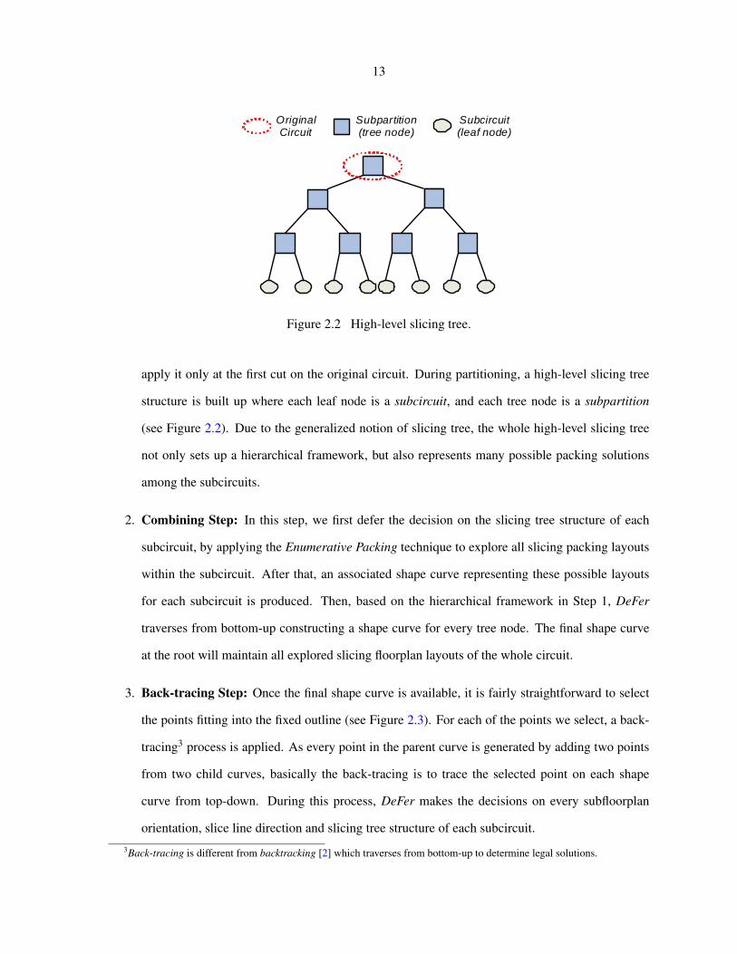
Figure 2.2 High-level slicing tree.
apply it only at the first cut on the original circuit. During partitioning, a high-level slicing tree
structure is built up where each leaf node is a subcircuit, and each tree node is a subpartition
(see Figure 2.2). Due to the generalized notion of slicing tree, the whole high-level slicing tree
not only sets up a hierarchical framework, but also represents many possible packing solutions
among the subcircuits.
2. Combining Step: In this step, we first defer the decision on the slicing tree structure of each
subcircuit, by applying the Enumerative Packing technique to explore all slicing packing layouts
within the subcircuit. After that, an associated shape curve representing these possible layouts
for each subcircuit is produced. Then, based on the hierarchical framework in Step 1, DeFer
traverses from bottom-up constructing a shape curve for every tree node. The final shape curve
at the root will maintain all explored slicing floorplan layouts of the whole circuit.
3. Back-tracing Step: Once the final shape curve is available, it is fairly straightforward to select
the points fitting into the fixed outline (see Figure 2.3). For each of the points we select, a back-
tracing3 process is applied. As every point in the parent curve is generated by adding two points
from two child curves, basically the back-tracing is to trace the selected point on each shape
curve from top-down. During this process, DeFer makes the decisions on every subfloorplan
orientation, slice line direction and slicing tree structure of each subcircuit.3Back-tracing is different from backtracking [2] which traverses from bottom-up to determine legal solutions.
14
Final shape curveFixed outline
W
H
(0, 0)
Valid solutions
Figure 2.3 Final shape curve with fixed outline and candidate points.
4. Swapping Step: The fourth step is to make decisions on the subfloorplan order (left-right/top-
bottom), by greedily swapping every two child subfloorplans. Basically we perform three wire-
length refinement processes through the hierarchical framework. First, Rough Swapping is ap-
plied from top-down, followed by Detailed Swapping. Finally, we apply Mirroring.
5. Compacting Step: After fixing the slicing floorplan, this step is to compact all modules to the
center of the fixed outline. The compaction puts modules closer to each other, such that the wire-
length is further reduced. If the slicing floorplan is outside of the fixed outline, DeFer compacts
them to the lower-left corner rather than the center, so that potentially there is a higher chance to
find a valid layout within the fixed outline.
6. Shifting Step: In Step 5, some modules may be over-compacted. So we greedily shift such
modules towards the optimal positions [35] regarding wirelength minimization. At the end, DeFer
outputs the final floorplan.
From the algorithm flow, we can see that by initially deferring the decisions in Steps 1 and 2, DeFer
explores a large collection of slicing layouts, all of which are efficiently maintained in one final shape
curve at the top; by finally making the decisions in Steps 3 and 4, DeFer chooses good slicing layouts
fitting into the fixed outline. The main techniques are discussed in detail in Sections 2.3-2.7.
15
A B
A B A B A B A B
A
B
A
B
AB
A
B
AB AB AB AB
A
BA
B
AB
A
B
Figure 2.4 Generalized slicing tree and sixteen different layouts.
2.3 Generalized Slicing Tree
In this section, we introduce the generalized slicing tree, which enables the deferred decisions on
these three factors: (1) Subfloorplan Orientation; (2) Subfloorplan Order; (3) Slice Line Direction.
2.3.1 Notion of Generalized Slicing Tree
In an ordinary slicing tree, the parent tree node of two child subfloorplans A and B is labeled
‘H’/‘V’ to specify that A and B are separated by a horizontal/vertical slice line, and the order between
the two child nodes in the slicing tree specifies the top-bottom/left-right order of A and B in the layout.
For example, if in the ordinary slicing tree the left child is A, the right child is B, and the parent node is
labeled ‘V’, then in the corresponding layout A is on the left of B. If we want to switch to other layouts
between A and B, then the slicing tree has to be changed as well.
Now we generalize the ordinary slicing tree, such that one generalized slicing tree represents mul-
tiple slicing layouts. Here we introduce a new operator — ‘⊕’ to incorporate both ‘H’ and ‘V’ slice
line directions. Moreover, we do not differentiate the ‘top-bottom’ or ‘left-right’ order between the two
child subfloorplans any more, which means even though we put A at the left child, it can be switched
to the right later on. We even do not specify the orientation for each subfloorplan. As a result, the de-
cisions on slice line direction, subfloorplan order, and subfloorplan orientation are deferred. Now each
parent node in the slicing tree represents all sixteen slicing layouts between two child subfloorplans (see
Figure 2.4).

16
W
A BH
Ch
W = H
W
H
C h
W = H
C v
W
H
C h
W = H
C v
(a) Addition (b) Flipping (c) Merging
k’k
C
Figure 2.5 Extended shape curve operation.
2.3.2 Extended Shape Curve Operation
To actualize the slicing tree combination we use the shape curve operation. The shape of each
subfloorplan is captured by its associated shape curve. In order to derive a compatible operation for the
new operator ‘⊕’, we develop three steps to combine two child curves A and B into one parent curve
C.
1. Addition: Firstly, we add two curves A and B horizontally to get curve Ch, on which each point
corresponds to a horizontal combination of two subfloorplan layouts from A and B, respectively
(see Figure 2.5 (a)).
2. Flipping: Next, we flip curve Ch symmetrically based on the W = H line to derive curve
Cv. The purpose of doing this is to generate the curve that contains the corresponding vertical
combination cases from the two subfloorplan layouts (see Figure 2.5 (b)).
3. Merging: The final step is to merge Ch and Cv into the parent curve C. Since the curve function
is a bijection from set W to set H , for a given height only one point can be kept. We choose the
point with a smaller width out of Ch and Cv, e.g., point k in Figure 2.5 (c), because such point
corresponds to smaller floorplan area.
As a result, we have derived three steps to actualize the operator ‘⊕’ in the slicing tree combination.
Now given two child curves corresponding to two child subfloorplans in the slicing tree, these three
steps are applied to combine the two curves into one parent curve, in which the entire slicing layouts
between the two child subfloorplans are captured.
17
2.3.3 Decision of Slice Line Direction for Terminal Propagation
Because all cut line directions in the high-level slicing tree are undetermined, we cannot apply Ter-
minal Propagation (TP) during partitioning. In order to enable TP, we pre-decide the cut line direction
based on the aspect ratio4 τp of the subpartition region. That is, if τp > 1, the subpartition will be
cut “horizontally”; otherwise, it will be cut “vertically”. In principle, we can use such strategy on all
cut lines in the high-level slicing tree. However, by doing this we restrict the combine direction in the
generalized slicing tree, which degrades the packing quality. To make a trade-off, we only apply TP at
the root, i.e., the first cut on the original circuit.
2.4 Whitespace-Aware Pruning
In this section, we present the Whitespace-Aware Pruning (WAP) technique, which systematically
prunes the points on the shape curve with whitespace awareness.
2.4.1 Motivation on WAP
In Figure 2.6 two subfloorplans A and B are combined into subfloorplan C. Shape curves Ca,
Cb and Cc contain various floorplan solutions of A, B and C, respectively. Because Cb has a gap
between points P2 and P3, during the combining process point P1 cannot find any point from Cb with
the matched height, and is forced to combined with P2. Due to the height difference between P1 and
P2, the resulted point P4 on curve Cc represents a layout with extra whitesapce. The bigger the gap is,
the more the whitespace is generated.
It is only an ideal situation that each point always had a matched point on another curve. Therefore,
in the hierarchical framework during the curve combining process, the whitespace will be generated and
accumulated to the top level. For a fixed-outline floorplanning problem, we have a budget/maximum
whitespace amount Wb. In order to avoid exceeding Wb, the whitespace generated in the curve combi-
nation needs to be minimized. One direct way to achieve this is to increase the number of points, such
that the sizes of gaps among the points are minimized. However, the more points we keep, the slower
the algorithm runs. This rises the question Whitespace-Aware Pruning (WAP) is trying to solve: How
4In this chapter, aspect ratio is defined as the ratio of height to width.

18
A
H
W
Ca Cb
B
HC c
No matched point Whitespace
P1
P4
P2
W
Gap
P3
Figure 2.6 Generation of whitespace during curve combination.
can we minimize the number of points on the shape curve, while guaranteeing that the total whitespace
would not exceed Wb?
2.4.2 Problem Formulation of WAP
WAP is to prune the points on the shape curve, while making sure that the gaps among the points are
small enough, such that we can guarantee the total whitespace would not exceed the budget Wb. WAP
is formulated as follows.
MinimizeM∑i=1
ki
subject toM∑i=1
Wpi +N∑j=1
Wcj +Wo ≤Wb
(2.1)
In Equation 2.1, suppose there are M subpartitions and N subcircuits in the high-level slicing tree (see
Figure 2.2). Before pruning, there are ki points on shape curve i of subpartition i. During the combine
process of generating shape curve i, the introduced whitespace in subpartition i is Wpi . The whitespace
inside subcircuit j isWcj . At the root, the whitespace between the floorplan outline and the fixed outline
is Wo.
To do pruning, we calculate a pruning parameter βi for shape curve i. In subpartition i, let the
corresponding width and height of point p (1 ≤ p ≤ ki) be wip and hip. On each shape curve, the points
are sorted based on the ascending order of the height. ∆Hp is defined for point p as follows.
∆Hp = βi · hip (2.2)
19
Within the distance of ∆Hp above point p, only the point that is the closest to hip + ∆Hp is kept, and
other points are pruned away. The intuition is that the gap within ∆Hp is small enough to guarantee
that no large whitespace will be generated. Such pruning method is applied only on every pair of child
curves of subpartitions in the high-level slicing tree, before they are combined into a parent curve. We
do not prune any point on the shape curves of subcircuits.
Now we rewrite Equation 2.1 into a form related with βi, such that by solving WAP we can get
the value of βi. Based on the above pruning, we have hip+1 ≤ (1 + βi) · hip. So approximately
hip+2 ≥ (1 + βi)hip. Thus, the relationship between the first point and point ki is:
hiki≥ (1 + βi)
ki−1
2 hi1 ⇒ ki ≤ 2 · (ln(hiki
/hi1)ln(1 + βi)
) + 1 (2.3)
Because of the Flipping (see Figure 2.5 (b)), each shape curve is symmetrical based on W = H line.
So in the implementation we only keep the lower half curve. In this case, the last point ki is actually
very close 5 to W = H line, so we have
wiki≈ hiki
⇒ hiki≈
√Ai (2.4)
where Ai is the area of subpartition i. It equals to the sum of total module area in subpartition i and
the accumulated whitesapce from the subcircuits at lower level. In Equation 2.3, hi1 is actually the
minimum height of the outlines on shape curve i. Suppose subpartition i contains Vi modules. The
width and height of module m are xim and yim.
hi1 = max(min(xi1, yi1), · · · ,min(xiVi
, yiVi)) (2.5)
In the following part, we explain the calculation of other terms in Equation 2.1.
• Calculation of Wpi
Suppose two child subpartitions Si1 and Si2 are combined into parent subpartition Si, where the
area of Si1, Si2 and Si are Ai1, Ai2 and Ai. The pruning parameter of Si is βi. As shown in
Figure 2.7 (a), the whitespace produced in the combining process is
Wpi = Ai ·Ai2 · βi
Ai1 +Ai2 +Ai2 · βi(2.6)
5If ki represents a outline of a square, it is on W = H line.

20
H
W
S1i
S2i
ßi
1
Wpi
W
H
(b)
S1
P1
Pd
W o
(a)
Figure 2.7 Calculation of Wpi and Wo.
Since the partitioner tries to balance the area of Si1 and Si2, we can assume Ai1 ≈ Ai2. Typically
βi � 2, so Ai1 +Ai2 +Ai2 · βi ≈ Ai. Thus,
Wpi = Ai1 · βi = Ai2 · βi = Ai ·βi2
(2.7)
• Calculation of Wcj
Before pruning, the shape curves of subcircuits have already been generated by EP. We choose the
minimum whitespace among all layouts of subcircuit j as the value of Wcj , so that∑N
j=1Wcj ≥
Wb can be prevented.
• Calculation of Wo
At the root, there is extra whitespace Wo between the floorplan outline and the fixed outline.
DeFer picks at most δ points (δ = 21 by default) for Back-tracing Step. So we assume there are
δ points enclosed into the fixed outline, and the first and last points P1, Pd out of δ are on the
right and top boundary of the fixed outline (see Figure 2.7 (b)). For various points/layouts, Wo is
different. We use the one of P1 to approximate Wo. As in pruning we always keep the point that
is the closest to (1 + βi)hip, here we can assume h1p+1 = (1 + β1)h1
p. So we have
Wo = A1 · ((1 + β1)δ−1 − 1) (2.8)
21
From Equations 2.3, 2.4, 2.7, 2.8, Equation 2.1 can be rewritten as:
MinimizeM∑i=1
ln(√Ai/h
i1)
ln(1 + βi)
subject toM∑i=1
Ai ·βi2
+N∑j=1
Wcj +Wo ≤Wb
Wo = A1 · ((1 + β1)δ−1 − 1)
βi ≥ 0 i = 1, . . . ,M
(2.9)
2.4.3 Solving WAP
To solve WAP (Equation 2.9), we relax the constraint related withWb by Lagrangian relaxation. Let
λ be the non-negative Lagrange multiplier, and W ′ = Wb −∑N
j=1Wcj −Wo.
Lλ(βi) =M∑i=1
ln(√Ai/h
i1)
ln(1 + βi)+ λ · (
M∑i=1
Ai ·βi2−W ′)
LRS : Minimize Lλ(βi)
subject to βi ≥ 0 i = 1, . . . ,M
LRS is the Lagrangian relaxation subproblem associated with λ. Let the function Q(λ) be the optimal
value of LRS. The Lagrangian dual problem (LDP) is defined as:
LDP : Maximize Q(λ)
subject to λ ≥ 0
As WAP is a convex problem, if λ is the optimal solution of LDP, then the optimal solution of LRS also
optimizes WAP. We differentiate Lλ(βi) based on βi and λ, respectively.
∂L
∂β1= λA1(
12
+ (δ − 1) · ((1 + β1)δ−2))− ln(√A1/h
11)
(1 + β1) · ln2(1 + β1)
∂L
∂βi=λAi
2− ln(
√Ai/h
i1)
(1 + βi) · ln2(1 + βi), i = 2, . . . ,M
∂L
∂λ=
M∑i=1
Ai ·βi2−W ′
To find the “saddle point” between LRS and LDP, we first set an arbitrary λ. Once λ is fixed, ∂L∂βi
(1 ≤ i ≤M ) is a univariate function that can be solved by Bisection Method to get βi. Then βi is used

22
to get the value of function ∂L∂λ . If ∂L
∂λ 6= 0, we adjust λ accordingly based on Bisection Method and do
another iteration of the above calculation, until ∂L∂λ = 0.
Eventually, the pruning parameters βi returned by WAP are used to systematically prune the points
on the shape curve of each subpartition i. Best of all, we do not need to worry about the over-pruning
and degradation of the packing quality.
2.5 Enumerative Packing
In order to defer the decision on the slicing tree structure, we propose the Enumerative Packing (EP)
technique that can efficiently enumerate all possible slicing layouts among a set of modules, and finally
keep all of them into one shape curve.
2.5.1 A Naive Approach of Enumeration
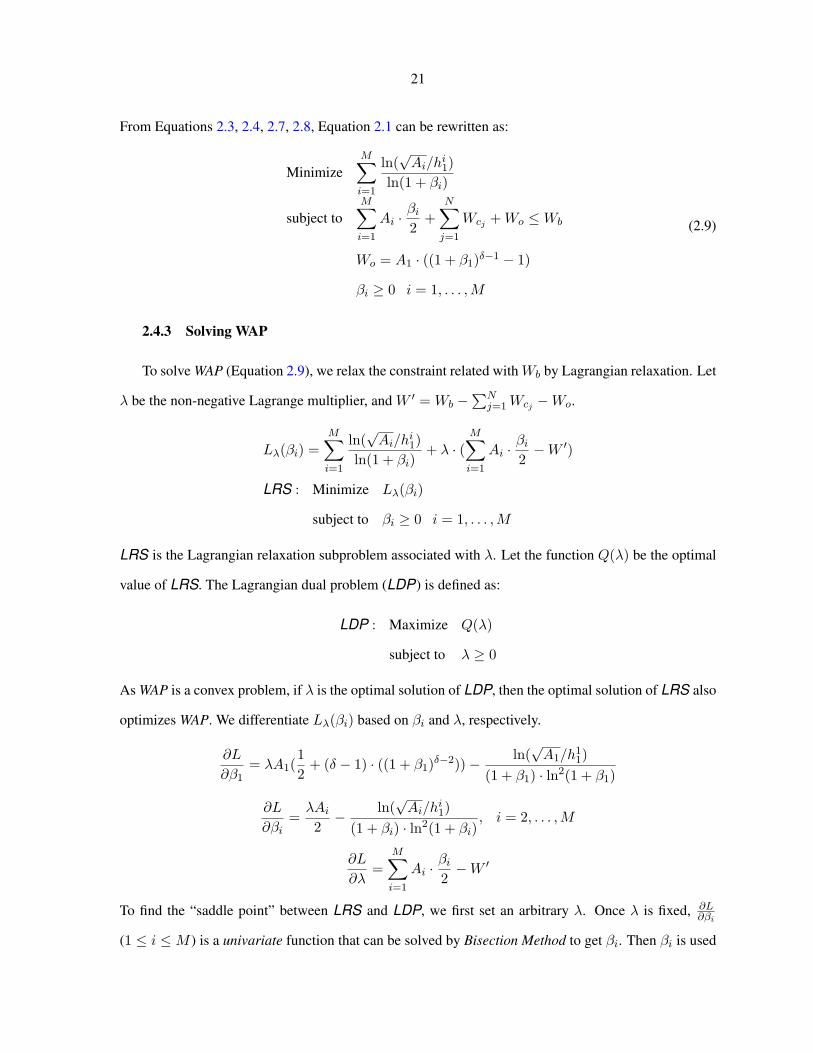
In this subsection, we plot out a naive way to enumerate all slicing packing solutions among n
modules. We first enumerate all slicing tree structures and then enumerate all permutations of the
modules. Let L(n) be the number of different slicing tree structures for n modules. So we have
L(n) =bn
2c∑
i=1
L(n− i) · L(i) (2.10)
All slicing tree structures for 3 to 6 modules are listed in Figure 2.8. Note that we are using the
generalized slicing tree which does not differentiate the left-right order between two child subtrees. As
we can see the number of different slicing tree structures is actually very limited.
To completely explore all slicing packing solutions among nmodules, for each slicing tree structure,
different permutations of the modules should also be considered. For example in Figure 2.8, in tree T4a
four modules A, B, C and D can be mapped to leaves “1− 2− 3− 4” by the order “A−B−C −D”
or “A−C−B−D”. Obviously these two orders derive two different layouts. However, again because
the generalized slicing tree does not differentiate the left-right order between two child subtrees which
share the same parent node, for example, orders “A−B −C −D” and “B −A−C −D” are exactly
the same in T4a. After pruning such redundancy, we have 4!2 = 12 non-redundant permutations for
mapping four modules to the four leaves in T4a. Therefore, for each slicing tree structure of n modules,
23
3
1 2
1 2
3
4
1 2 3 4
1 2
3
4
5
6
1 2 3 4
5
6
3
1 2
4 5
6
1 2
3
4 5 6
1 2 3 4
5 6 3
1 2
6
4 5
1 2
3
4
5
1 2 3 4
5
3
1 2
4 5
T4a T4b T5a T5b T5c
T6a T6b T6c T6d T6e T6f
T3
Figure 2.8 List of different slicing tree structures.
we first enumerate all non-redundant permutations, for each one of which a shape curve is produced.
And then we merge these curves into one curve associated with each slicing tree structure. Finally, these
curves from all slicing tree structures are merged into one curve that captures all possible slicing layouts
among these nmodules. To show the amount of computations in this process, we list the number of ‘⊕’
operations for different numbers of modules in the second column of Table 2.1.
2.5.2 Enumeration by Dynamic Programming
Table 2.1 shows that the naive approach can be very expensive in both runtime and memory usage.
Alternatively, we notice that the shape curve for a set of modules (M) can be defined recursively by
Equation 2.11 below.
S(M) = MERGEA⊂M,B=M−A
(S(A)⊕ S(B)) (2.11)
S(M) is the shape curve capturing all slicing layouts among modules in M , MERGE() is similar to the
Merging in Figure 2.5 (c), but operates on shape curves from different sets.
Based on Equation 2.11, we can use Dynamical Programming (DP) to implement the shape curve
generation. First of all, we generate the shape curve representing the outline(s) of each module. For hard
modules, there are two points6 in each curve. For soft modules, only several points from each original6One point if the hard module is a square.

24
Table 2.1 Comparison on # of ‘⊕’ operation.
n # of ⊕ # of ⊕by naive approach with DP
2 1 13 6 64 45 255 400 906 4,155 3017 49,686 9668 674,877 3,0259 10,295,316 9,330
10 174,729,015 28,501
curve are evenly sampled7. And then starting from the smallest subset of modules, we proceed to build
up the shape curves for the larger subsets step by step, until the shape curve S(M) is generated. Since
in this process the previously generated curves can be reused for building up the curves of larger subsets
of modules, many redundant computations are eliminated. After applying DP, the resulted numbers of
‘⊕’ operations are listed in the third column of Table 2.1.
2.5.3 Impact of EP on Packing
To control the quality of packing in EP, we can adjust the number of modules in the set. Con-
sequently the impact on packing is: The more modules a set contains, the more different slicing tree
structures we explore, the more slicing layout possibilities we have, and thus the better quality of pack-
ing we will gain at the top level.
However, if the set contains too many modules, two problems appear in EP: 1) The memory to
store results from subsets can be expensive; 2) Since the interconnections among the modules are not
considered, the wirelength may be increased. Due to these two concerns, in the first step of DeFer,
we apply hMetis to recursively cut the original circuit into multiple smaller subcircuits. This process
not only helps us to cut down the number of modules in each subcircuit, but initially optimizes the
wirelength as well. Later on as applying EP on each subcircuit, the wirelength would not become a
big concern, because this is only a locally packing exploration among a small number of modules. In
7The number of sampled points on the whole curve is determined by bAiA0ρc+ 4, where Ai is the area of soft block i, A0
is the total block area, and ρ is a constant (ρ = 10000 by default).

25
other words, in the spirit of DDM, instead of deferring the decision on the slicing tree structure among
all modules in the original circuit, first we fix the high-level slicing tree structure among the subcircuits
by partitioning, and then defer the decision on the slicing tree structure among the modules within each
subcircuit.
2.5.4 High-Level EP
In the modern SoC design, the usage of Intellectual Property (IP) becomes more and more popular.
As a result, a circuit usually contains numbers of big hard macros. Due to the big size differences from
other small modules, they may produce some large whitespace. For example in Figure 2.9 (a), after
partitioning, the original circuit has been cut into four subcircuitsA, B, C andD. A contains a big hard
macro. Respecting the slicing tree structure of T4b, you may find that no matter how hard EP explores
various packing layouts within A or B, there is always a large whitespace, such as Q, in the parent
subfloorplan. This is because the high-level slicing tree structure among subcircuits has been fixed by
partitioning, so that some small subcircuit is forced to combine with some big subcircuit. Thus, to solve
this problem, we need to explore other slicing tree structures among the subcircuits.
To do so, we apply EP on a set of subfloorplans, instead of a set of modules. As the input of EP
is actually a set of shape curves, and shape curves can represent the shape of both subfloorplans and
modules, it is capable of using EP to explore the layouts among subfloorplans. In Figure 2.9 (b), EP is
applied on the four shape curves coming from subfloorplans A, B, C and D, respectively. So all slicing
tree structures (T4a and T4b) and permutations among these subfloorplans can be completely explored.
Eventually one tightly-packed layout can be chosen during Back-tracing Step (see Figure 2.9 (c)).
Before we describe the criteria of triggering high-level EP, some concepts are introduced here:
• Big gap : Based on the definition of ∆Hp in Section 2.4, if hip+1 − hip > ω · ∆Hp (ω is “Gap
Ratio”, ω = 5 by default), then we say there is a “big gap” between points p and p+1. Intuitively,
if there is a big gap, most likely it would cause serious packing problem at upper level.
• hNode : In the high-level slicing tree, the tree node or leaf node that contains big gap(s).
• hTree : A subtree of the high-level slicing tree, where the high-level EP is applied. For example,
26
Big Macro
T4b T4a
Big Macro
AB
CD
A
B
C
D
High-LevelEP
T4aT4b
Big Macro
A
B C D(a) (b) (c)
Big Macro
Q
Figure 2.9 Illustration of high-level EP.
T4b is a hTree (see Figure 2.9 (a)).
• hRoot : The root node of hTree.
High-level EP is to solve the packing problem caused by big gaps, so we need to identify the hTree
that contains big gap. First we search for the big gap through the high-level slicing tree. If any shape
curve has a big gap, then the corresponding node becomes a hNode. After identifying all hNodes, each
hNode becomes a hRoot, and the subtree whose root node is hRoot becomes a hTree. But there is one
exception: as shown in Figure 2.10, if one hTree T2 is a subtree of another hTree T1, then T2 will not
become a hTree. Eventually, each hTree contains at least one big gap, which implies critical packing
problems. Thus, for every hTree we use high-level EP to further explore the various packing layouts
among the subfloorplans, i.e., leaves of hTree. If a hTree has more than 10 leaves, we will combine
them from bottom-up until the number of leaves becomes 10.
As mentioned in Section 2.5.3, EP only solves the packing issue, which may degrade the wirelength.
Therefore, to make a trade-off we apply high-level EP only if there is no point enclosed into the fixed
outline after Combining Step. If that is the case, then we will use the above criteria to trigger the
high-level EP, and reconstruct the final shape curve.

27
T2
T1T1
Tree node hRoot hTree
Figure 2.10 One exception of identifying hTree.
2.6 Block Swapping and Mirroring
After Back-tracing Step, the decision on subfloorplan order (left-right/top-bottom) has not been
made yet. Using such property, this section focuses on optimizing the wirelength.
In slicing structures switching the order (left-right/top-bottom) of two child subfloorplans would
not change the dimension of their parent floorplan outline, but it may actually improve the wirelength.
Basically, we adopt three techniques here: (1) Rough Swapping; (2) Detailed Swapping; (3) Mirroring.
Each of them is trying to switch the positions of two subfloorplans to improve the HPWL. Figure 2.11
illustrates the differences between Swapping and Mirroring. In Swapping we try to switch the left
and right subfloorplans, inside of which the relative positions among the modules are unchanged. In
Mirroring, instead of simply swapping two subfloorplans, we first figure out the symmetrical axis of the
outline at their parent floorplan, and then attempt to mirror them based on this axis. When calculating
the HPWL, in Rough Swapping we treat all internal modules to be at the center of their subfloorplan
outline. In Detailed Swapping we use the actual center coordinates of each module in calculating the
HPWL.
Rough Swapping is an essential step before Detailed Swapping. Without it, the results produced
by Detailed Swapping could degrade the wirelength. For example in Figure 2.12, when we try to swap
two subfloorplans A and B, two types of nets need to be considered: internal nets neti between A and
B, and external nets neto between the modules inside A or B and other outside modules or fixed pads.
Let C and D be two modules inside A and B, respectively. C and D are highly connected by netcd.
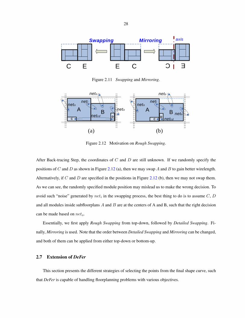
28
Swapping Mirroring
EC E C
EC
axis
Figure 2.11 Swapping and Mirroring.
A BC
D
neti
A BC
D
(a) (b)
neto
netcd
neto
neto neto
neto
neto
neti
netcd
Figure 2.12 Motivation on Rough Swapping.
After Back-tracing Step, the coordinates of C and D are still unknown. If we randomly specify the
positions of C andD as shown in Figure 2.12 (a), then we may swapA andB to gain better wirelength.
Alternatively, if C and D are specified in the positions in Figure 2.12 (b), then we may not swap them.
As we can see, the randomly specified module position may mislead us to make the wrong decision. To
avoid such “noise” generated by neti in the swapping process, the best thing to do is to assume C, D
and all modules inside subfloorplans A and B are at the centers of A and B, such that the right decision
can be made based on neto.
Essentially, we first apply Rough Swapping from top-down, followed by Detailed Swapping. Fi-
nally, Mirroring is used. Note that the order between Detailed Swapping and Mirroring can be changed,
and both of them can be applied from either top-down or bottom-up.
2.7 Extension of DeFer
This section presents the different strategies of selecting the points from the final shape curve, such
that DeFer is capable of handling floorplanning problems with various objectives.
29
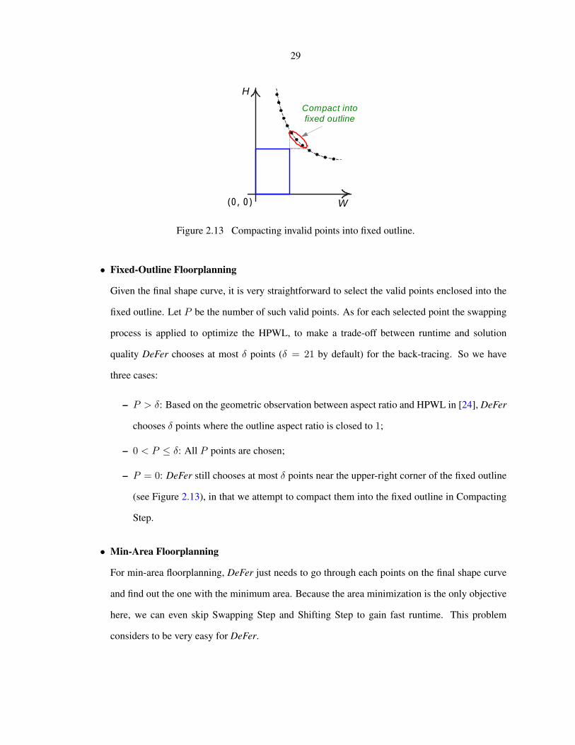
W
H
(0, 0)
Compact into fixed outline
Figure 2.13 Compacting invalid points into fixed outline.
• Fixed-Outline Floorplanning
Given the final shape curve, it is very straightforward to select the valid points enclosed into the
fixed outline. Let P be the number of such valid points. As for each selected point the swapping
process is applied to optimize the HPWL, to make a trade-off between runtime and solution
quality DeFer chooses at most δ points (δ = 21 by default) for the back-tracing. So we have
three cases:
– P > δ: Based on the geometric observation between aspect ratio and HPWL in [24], DeFer
chooses δ points where the outline aspect ratio is closed to 1;
– 0 < P ≤ δ: All P points are chosen;
– P = 0: DeFer still chooses at most δ points near the upper-right corner of the fixed outline
(see Figure 2.13), in that we attempt to compact them into the fixed outline in Compacting
Step.
• Min-Area Floorplanning
For min-area floorplanning, DeFer just needs to go through each points on the final shape curve
and find out the one with the minimum area. Because the area minimization is the only objective
here, we can even skip Swapping Step and Shifting Step to gain fast runtime. This problem
considers to be very easy for DeFer.

30
• Min-Area and Wirelength Floorplanning
This problem uses a linear combination of area and wirelength as the cost function. Compared
with the strategy of fixed-outline floorplanning, the only difference is that we just need to choose
the δ points with the minimum area, rather than within the fixed outline.
As shown above, DeFer is very easy to be switched to handle other floorplanning problems. Be-
cause once the final shape curve is available, DeFer has provided a large amount of floorplan candidates.
Given any objective function, e.g., that used in simulated annealing, we just need to evaluate the candi-
dates, and pick the one that gives the minimum cost.
2.8 Implementation Details
Sometimes DeFer cannot pack all modules into the fixed outline. This may occur because hMetis
generates a hard-to-pack partition result, or the packing strength is not strong enough. To enhance the
robustness of DeFer, we adaptively tune some parameters and try another run.
One effective way to improve the packing quality of DeFer is to enhance the packing strength in the
high-level EP, e.g., by decreasing the gap ratio ω. Also we can use different strategies to identify hRoot
(see Figure 2.14):
(a) Each hNode becomes a hRoot.
(b) Each hNode’s grandparent tree node becomes a hRoot.
Strategy (a) is the one we mentioned in Section 2.5.4. Apparently, if we adopt strategy (a), more hTrees
will be generated, and thus the high-level EP is used more often, which leads better packing. However,
this takes longer runtime.
Another way to improve the packing quality is to balance both the area and number of modules,
rather than only the area in each partition at Partitioning Step. Thus we have two methods to set the
weight for the module.
(a) Wgt = Am
(b) Wgt = Am + 0.6 ·Ap

31
Tree node hNode hRoot
( a ) ( b )
Figure 2.14 Two strategies of identifying hRoot.
S : hMetis Initial Seed, GR : Gap Ratio, HS : hRoot Strategy,W : Weight Setting Method**** Quit any run, once satisfy fixed-outline constraint ****Run 1: hMetis(S), GR = 5, HS = (b), W = (a)Run 2: hMetis(S++), GR = 5, HS = (b), W = (a)Run 3: GR = 5, HS = (a)Run 4: GR = 4, HS = (a)Run 5: GR = 3, HS = (a)Run 6: hMetis(S++), GR = 3, HS = (a), W = (b)Run 7: hMetis(S++), GR = 3, HS = (a), W = (b)Run 8: hMetis(S++), GR = 3, HS = (a), W = (b)
Figure 2.15 Tuned parameters at each run in DeFer.
where Wgt and Am are the weight and area for module m, Ap is the average module area in partition
p. In experiments we observe that method (b), which considers both the area and number of modules,
generates better packing results, yet sacrifices the wirelength.
Essentially, DeFer starts with the defaulted parameters for the first run. If failing to pack all modules
into the fixed outline, it will internally enhance the packing strength and try another run. By default
DeFer will try at most 8 runs. The tuned parameters for each run is listed in Figure 2.15. For Run 3–5
because they share the same partition result with Run 2, DeFer skips Partitioning Step in those runs.
Even though DeFer internally executes multiple runs, it still achieves the best runtime compared
with all other floorplanners. There are two reasons: (1) DeFer is so fast. Even it runs multiple times,
it is still much faster than other floorplanners. (2) DeFer has better packing quality. For most circuits,
32
DeFer can satisfy the fixed-outline constraint within Run 1.
2.9 Experimental Results
In this section, we present the experimental results. All experiments were performed on a Linux
machine with Intel Core Duo8 1.86 GHz CPU and 2GB memory. The wirelength is measured by
HPWL. We compare DeFer with all the best publicly available state-of-the-art floorplanners, of which
the binaries are the latest version. For the hMetis 1.5 parameters in DeFer, NRuns = 1, UBfactor = 10,
and others are defaulted.
2.9.1 Experiments on Fixed-Outline Floorplanning
In this subsection, we compare DeFer with other fixed-outline floorplanners. On GSRC [36] and
HB [37] benchmarks, for each circuit we choose 3 different fixed-outline aspect ratios: τ = 1, 2, 3. All
I/O pads are scaled to the according boundary. On HB+ benchmarks, we use the defaulted fixed outlines
and I/O pad locations. By default every floorplanner runs 100 times for each test case, and the results are
averaged over all successful runs. As PATOMA has internally fixed the hMetis seed, and produces the
same result no matter how many times it runs, we run it only once. For other floorplanners, the initial
seed is the same as the index of each run. Parquet 4.5 runs in wirelength minimization mode. The
parameters for other floorplanners are defaulted. For each type of benchmarks, we finally normalize all
results to DeFer’s results.
I. GSRC Hard-Block Benchmarks These circuits contain 100, 200 and 300 hard modules. De-
Fer compares with six floorplanners: Parquet 4.5[20], FSA[21], IMF[23], IARFP[24], PATOMA[29]
and Capo 10.5[2]. The maximum whitespace percentage γ = 10%. The results are summarized in
Table 2.2. For every test case DeFer reaches 100% success rate. DeFer generates 27%, 14%, 14%,
3%, 25% and 5% better HPWL in 181×, 558×, 158×, 64×, 15% and 222× faster runtime than Par-
quet 4.5, FSA, IMF, IARFP, PATOMA and Capo 10.5, respectively. DeFer consistently achieves the
best HPWL and best runtime on all 9 test cases, except for only one case (n100, τ = 3) DeFer gen-
erates 0.5% worse HPWL than IARFP. But for that one DeFer is 41× faster than IARFP with 100%8In the experiments, only one core was used.

33
success rate. Figures 2.16(a), 2.16(b) and 2.16(c) show the layouts produced by DeFer on circuit n300
with τ = 1, 2, 3.
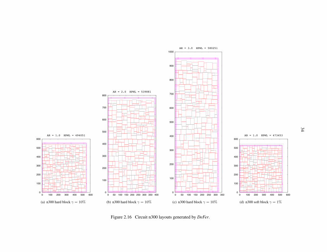
34
0
100
200
300
400
500
600
0 100 200 300 400 500 600
AR = 1.0 HPWL = 494051
(a) n300 hard block γ = 10%
0
100
200
300
400
500
600
700
800
0 50 100 150 200 250 300 350 400
AR = 2.0 HPWL = 539881
(b) n300 hard block γ = 10%
0
100
200
300
400
500
600
700
800
900
1000
0 50 100 150 200 250 300 350
AR = 3.0 HPWL = 580251
(c) n300 hard block γ = 10%
0
100
200
300
400
500
600
0 100 200 300 400 500 600
AR = 1.0 HPWL = 473453
(d) n300 soft block γ = 1%
Figure 2.16 Circuit n300 layouts generated by DeFer.

35
Table 2.2 Comparison on GSRC Hard-Block benchmarks (γ = 10%).
Circuit n100 n200 n300 Normal-Aspect Ratio 1 2 3 1 2 3 1 2 3 lized
Parquet 4.5 42% 43% 33% 26% 19% 17% 16% 16% 14% 0.25FSA 100% 0% 0% 100% 0% 0% 0% 0% 0% 0.22IMF 100% 100% 100% 100% 100% 100% 100% 100% 100% 1.00
Suc% IARFP 99% 100% 99% 100% 99% 63% 100% 100% 46% 0.90PATOMA 0% 0% 0% 0% 100% 0% 100% 100% 100% 0.44Capo 10.5 17% 17% 15% 0% 0% 2% 0% 1% 0% 0.06
DeFer 100% 100% 100% 100% 100% 100% 100% 100% 100% 1Parquet 4.5 248652 269191 289963 467627 506946 544621 686588 725833 781556 1.27
FSA 243823 — — 414777 — — — — — 1.14IMF 250680 251418 257935 438467 454231 482651 584578 617510 666245 1.14
HPWL IARFP 220269 230553 247283 386537 409208 433631 535850 567496 600438 1.03PATOMA — — — — 483110 — 653711 697740 680671 1.25Capo 10.5 227046 241789 261334 — — 444079 — 566998 — 1.05
DeFer 208650 229603 248567 372546 402155 431552 498909 538515 577209 1Parquet 4.5 10.85 10.58 10.27 44.43 44.47 41.96 95.02 87.03 86.31 181.49
FSA 39.78 — — 202.13 — — — — — 557.74IMF 7.65 10.82 9.29 41.21 43.59 38.71 74.74 71.48 71.72 157.91
Time(s) IARFP 4.44 4.50 4.52 16.51 15.48 14.22 29.30 29.48 30.03 64.33PATOMA — — — — 0.25 — 0.36 0.34 0.48 1.15Capo 10.5 122.64 125.18 160.07 — — 3054 — 8661 — 222.39
DeFer 0.13 0.11 0.11 0.25 0.23 0.22 0.35 0.33 0.33 1#Valid Point / #Total Point 3 / 617 4 / 621 3 / 621 3 / 670 2 / 672 2 / 672 6 / 869 5 / 869 4 / 869

36
II. GSRC Soft-Block Benchmarks These circuits contain 100, 200, and 300 soft modules. DeFer
compares with Parquet 4.5, Capo 10.5 and PATOMA, as only these floorplanners can handle soft mod-
ules. We add “-soft” to Parquet 4.5 command line. The maximum whitespace percentage γ = 1%,
which is almost zero whitespace requirements. As we can see from Table 2.3, after 100 runs both Par-
quet 4.5 and Capo 10.5 cannot pack all modules within the fixed outline. PATOMA and DeFer reach
100% success rate on every test case. Compared with PATOMA, DeFer generates 1% better wirelength
with 4× faster runtime. Figure 2.16(d) is the final layout generated by DeFer on circuit n300 with
τ = 1, which shows almost 0% whitespace is reached.
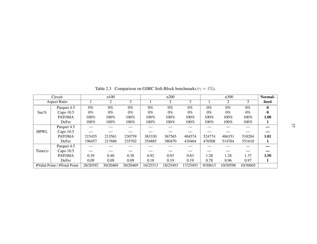
37
Table 2.3 Comparison on GSRC Soft-Block benchmarks (γ = 1%).
Circuit n100 n200 n300 Normal-Aspect Ratio 1 2 3 1 2 3 1 2 3 lized
Parquet 4.5 0% 0% 0% 0% 0% 0% 0% 0% 0% 0Suc% Capo 10.5 0% 0% 0% 0% 0% 0% 0% 0% 0% 0
PATOMA 100% 100% 100% 100% 100% 100% 100% 100% 100% 1.00DeFer 100% 100% 100% 100% 100% 100% 100% 100% 100% 1
Parquet 4.5 — — — — — — — — — —HPWL Capo 10.5 — — — — — — — — — —
PATOMA 215455 213561 230759 383330 367565 404574 524774 486351 518204 1.01DeFer 196457 217686 235702 354885 380470 410464 476508 514764 551610 1
Parquet 4.5 — — — — — — — — — —Time(s) Capo 10.5 — — — — — — — — — —
PATOMA 0.39 0.40 0.38 0.92 0.93 0.83 1.28 1.28 1.37 3.50DeFer 0.09 0.09 0.09 0.18 0.19 0.19 0.78 0.96 0.97 1
#Valid Point / #Total Point 28/20392 30/20469 30/20469 16/25513 18/25493 17/25493 9/30613 10/30598 10/30603
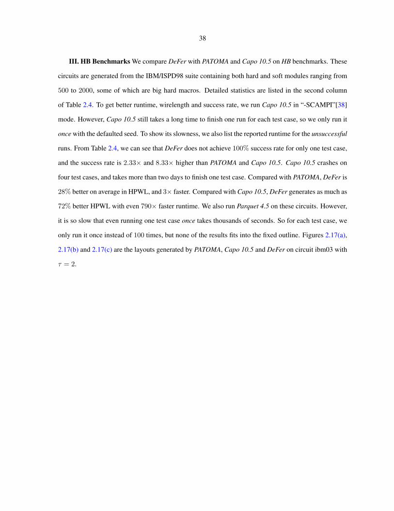
38
III. HB Benchmarks We compare DeFer with PATOMA and Capo 10.5 on HB benchmarks. These
circuits are generated from the IBM/ISPD98 suite containing both hard and soft modules ranging from
500 to 2000, some of which are big hard macros. Detailed statistics are listed in the second column
of Table 2.4. To get better runtime, wirelength and success rate, we run Capo 10.5 in “-SCAMPI”[38]
mode. However, Capo 10.5 still takes a long time to finish one run for each test case, so we only run it
once with the defaulted seed. To show its slowness, we also list the reported runtime for the unsuccessful
runs. From Table 2.4, we can see that DeFer does not achieve 100% success rate for only one test case,
and the success rate is 2.33× and 8.33× higher than PATOMA and Capo 10.5. Capo 10.5 crashes on
four test cases, and takes more than two days to finish one test case. Compared with PATOMA, DeFer is
28% better on average in HPWL, and 3× faster. Compared with Capo 10.5, DeFer generates as much as
72% better HPWL with even 790× faster runtime. We also run Parquet 4.5 on these circuits. However,
it is so slow that even running one test case once takes thousands of seconds. So for each test case, we
only run it once instead of 100 times, but none of the results fits into the fixed outline. Figures 2.17(a),
2.17(b) and 2.17(c) are the layouts generated by PATOMA, Capo 10.5 and DeFer on circuit ibm03 with
τ = 2.

39
0
500
1000
1500
2000
2500
3000
3500
4000
4500
5000
0 500 1000 1500 2000 2500
HPWL = 12.94e+06
HH
H H
H
H
H
H
H H
H HHH H H
H HHH H
HHH H
H
HH H HH HH HH HHHH HH H H H HH HH H HHH H HH HH H HHHH HH HHHH H HHH HH
HHH HH HH HHHH HH H HH HHH HH HHHHH HHHH H HH HH HHH HH HH HHHH HH
H H H HH H H HH H HH HHH HH HH HHHH HHH HH HH H HHHHH HH HHH HH HH H HH
HHH H HH HHHH HH HHH HHH H HH HH H
HH HH HH HH H HH HHH HHH HH H HHH H
H HH H HHH H HHHHHHH HH HH HH HH H
HH H HH HHH H HHH HH H HH HH H HH HH
H H HH H HH H H HHHH HH HH HH H H HHH
(a) by PATOMA
0
500
1000
1500
2000
2500
3000
3500
4000
4500
5000
0 500 1000 1500 2000 2500
HPWL = 12.78e+06
(b) by Capo 10.5
0
500
1000
1500
2000
2500
3000
3500
4000
4500
5000
0 500 1000 1500 2000 2500
HPWL = 8.81e+06
HH
H
H
H
H
H
H
H
H
H H
H
H
H
H
HH
H
H
H
HH
H HH
H
H
H
HH
H
HH
H
H
HH
H
H
HH
H
H
HH
H
H
H
H H
H
H
HH
H
H
H
H
H
H
HH
H
H
H
H
H
H
H
H H
H
H
HH
H
H
H
H
H
H
H
H
H
H
H
H
HH
H
HH
H
H
H
H
H H
H
H
H
H
H
H
HH
H
H
HH
H
H
H
HH
H
H
H
H
H
H
H
H
H
H
H
H
H
H
H
H
H
H
H H
H
H
HH
H
H
H
H
H
H
H
H
H
H
H
HH
HH
H
H
H
H H
H
H
HH
H
H
H
H
H
HHHH
HH
H
H
HH
H
H
H
H
H H
H
H
H
HH
H
H
H
HH
HH
H
H
H
H
HH
H
H
HH
H
HH
H
H
H
HH
H
HH
H
H
H
H
H
H
H
H
H
H
H
H
H
HH
H
H
H
H
HH
H
H
HH
H
HH
HH
H
HH
HH
H
HHH
HH
H
HH
HH
HH
HH
H
H
HH
HH
H
H
H
HHH
HHH
H
H
H
H
H
H
H
(c) by DeFer
Figure 2.17 Circuit ibm03 layouts generated by PATOMA, Capo 10.5 and DeFer (γ = 10% andτ = 2).

40
Table 2.4 Comparison on HB benchmarks (γ = 10%).
Circuit #Soft./#Hard. Aspect PATOMA[29] Capo 10.5[2] DeFer #Valid Point/#Net. Ratio Suc% WL(e6) Time(s) Suc% WL(e6) Time(s) Suc% WL(e6) Time(s) / #Total Point
665 1 100% 2.84 7.04 0% — 183 100% 2.66 1.44 16 / 1571ibm01 /246 2 0% — — 0% — 977 100% 2.70 1.28 11 / 1482
/4236 3 100% 5.60 1.66 0% — 696 100% 2.82 1.30 12 / 14901200 1 0% — — 0% — 456 85% 6.55 14.48 6 / 2348
ibm02 /271 2 0% — — — — > 2 days 100% 6.21 3.33 7 / 1161/7652 3 0% — — 0% — 3726 100% 6.29 3.52 10 / 1144999 1 100% 12.59 5.42 100% 10.70 566 100% 8.77 3.60 59 / 2684
ibm03 /290 2 100% 12.94 5.58 100% 12.01 1874 100% 8.89 3.49 40 / 2503/7956 3 0% — — 0% — 2028 100% 8.99 3.59 44 / 26301289 1 0% — — 0% — 2752 100% 8.94 3.04 4 / 1492
ibm04 /295 2 0% — — 100% 17.77 5253 100% 8.96 3.12 9 / 1514/10055 3 0% — — 100% 16.32 2262 100% 9.64 6.31 12 / 2685
564 1 100% 12.27 14.21 0% — 458 100% 12.61 3.55 46 / 3369ibm05 /0 2 100% 12.60 13.68 0% — 358 100% 12.73 3.52 46 / 3371
/7887 3 100% 13.19 13.85 0% — 411 100% 13.45 3.53 46 / 3371571 1 0% — — 0% — 235 100% 7.87 3.66 53 / 2187
ibm06 /178 2 0% — — 0% — 592 100% 7.76 3.66 41 / 2235/7211 3 0% — — 0% — 2831 100% 8.91 3.60 36 / 2196829 1 0% — — 0% — 1094 100% 13.81 3.87 12 / 1527
ibm07 /291 2 100% 24.64 7.85 0% — 1270 100% 13.91 4.48 22 / 1625/11109 3 100% 24.34 8.68 0% — 2274 100% 14.32 4.26 18 / 1590
968 1 0% — — 0% — 2527 100% 13.95 5.44 15 / 1333ibm08 /301 2 0% — — 0% — 1110 100% 14.16 5.40 17 / 1290
/11536 3 0% — — 0% — 1958 100% 14.43 5.55 19 / 1309860 1 0% — — 0% — 2273 100% 12.85 2.60 3 / 1495
ibm09 /253 2 0% — — 0% — 2670 100% 12.57 3.77 17 / 1486/11008 3 0% — — 100% 34.48 6652 100% 12.98 3.54 14 / 1486
41
Table 2.4 (Continued)
Comparison on HB benchmarks (γ = 10%).Circuit #Soft./#Hard. Aspect PATOMA[29] Capo 10.5[2] DeFer #Valid Point
/#Net. Ratio Suc% WL(e6) Time(s) Suc% WL(e6) Time(s) Suc% WL(e6) Time(s) / #Total Point
809 1 100% 48.47 21.71 0% — 2353 100% 33.25 11.63 9 / 2576ibm10 /786 2 0% — — crashed crashed crashed 100% 34.23 18.00 14 / 2897
/16334 3 0% — — 100% 53.64 2014 100% 36.59 16.52 9 / 27251124 1 100% 20.87 33.87 0% — 8070 100% 21.99 4.84 12 / 2218
ibm11 /373 2 0% — — 0% — 4732 100% 22.13 4.96 8 / 2207/16985 3 0% — — 0% — 2245 100% 22.83 4.67 7 / 2174
582 1 0% — — 0% — 3085 100% 29.72 10.95 20 / 2909ibm12 /651 2 0% — — 0% — 864 100% 31.53 7.71 18 / 3011
/11873 3 0% — — 0% — 19952 100% 32.16 4.59 8 / 1957530 1 0% — — 0% — 3401 100% 25.92 6.03 12 / 2553
ibm13 /424 2 100% 43.81 9.84 0% — 3662 100% 25.46 3.79 10 / 2048/14202 3 0% — — 0% — 3201 100% 26.47 3.83 8 / 20951021 1 100% 71.87 23.59 0% — 4253 100% 50.83 9.69 30 / 2976
ibm14 /614 2 100% 55.99 35.65 0% — 10373 100% 51.67 9.70 34 / 2971/26675 3 100% 61.65 35.12 0% — 4976 100% 53.71 9.70 36 / 29711019 1 0% — — 0% — 3634 100% 64.18 9.71 25 / 1651
ibm15 /393 2 0% — — 0% — 6827 100% 63.17 9.13 19 / 1580/28270 3 0% — — 0% — 2902 100% 66.06 9.46 20 / 1623
633 1 0% — — crashed crashed crashed 100% 56.88 16.79 18 / 3823ibm16 /458 2 100% 88.33 16.55 0% — 8928 100% 58.55 14.55 24 / 4833
/21013 3 100% 98.77 22.94 0% — 11675 100% 59.91 12.84 18 / 4093682 1 100% 102.45 41.75 crashed crashed crashed 100% 95.92 10.43 32 / 3253
ibm17 /760 2 100% 96.46 46.63 0% — 2250 100% 95.48 10.41 27 / 3252/30556 3 100% 98.18 42.45 crashed crashed crashed 100% 100.82 10.42 29 / 3252
658 1 100% 50.28 38.24 0% — 1083 100% 49.12 7.93 42 / 3106ibm18 /285 2 100% 49.74 39.15 0% — 4630 100% 49.29 7.97 41 / 3128
/21191 3 100% 52.26 36.97 0% — 5262 100% 51.39 7.97 41 / 3128Normalized 0.43 1.28 3.28 0.12 1.72 789.79 1 1 1

42
IV. HB+ Benchmarks DeFer compares with PATOMA and Capo 10.5 on HB+ benchmarks [38].
These circuits are generated from HB benchmarks, while the biggest hard macro is inflated by 100%
and the area of remaining soft macros are reduced to preserve the total cell area. As a result, the circuits
become even harder to handle. Due to the same reason, we set Capo 10.5 to “-SCAMPI” mode, and run
it only once. The results are shown in Table 2.5. DeFer achieves the 100% success rate on all circuits,
which is 1.89× better than PATOMA. Capo 10.5 also achieves 100% success rate, expect for one circuit
it takes more than two days to finish. In terms of the HPWL comparison, DeFer is 7% and 19% better
than PATOMA and Capo 10.5. DeFer is also 5× and 47× faster than PATOMA and Capo 10.5.
Both HB and HB+ benchmarks are considered to be very hard to handle, because these circuits not
only contain both hard and soft modules, but also big hard macros. As far as we know, only the above
floorplanners can handle these circuits. Obviously, DeFer reaches the best result. We also monitor the
memory usage of DeFer on such large-scale circuits, and observe that the peak memory usage in DeFer
is only 53 MB.

43
Table 2.5 Comparison on HB+ benchmarks.
Circuit White- Aspect PATOMA[29] Capo 10.5[2] DeFer #Valid Pointspace γ Ratio Suc% WL(e6) Time(s) Suc% WL(e6) Time(s) Suc% WL(e6) Time(s) / #Total Point
ibm01 26% 1 100% 4.67 4.44 — — > 2 days 100% 3.09 1.84 120 / 10860ibm02 25% 1 0% — — 100% 7.86 124 100% 6.17 15.28 45 / 3380ibm03 30% 1 0% — — 100% 12.75 343 100% 9.19 4.01 102 / 5020ibm04 25% 1 0% — — 100% 12.03 147 100% 10.26 14.15 63 / 5170ibm06 25% 1 0% — — 100% 10.09 155 100% 8.78 5.01 84 / 3560ibm07 25% 1 100% 16.38 23.41 100% 16.41 99 100% 15.48 4.55 12 / 3780ibm08 26% 1 0% — — 100% 18.29 284 100% 18.73 19.25 106 / 5070ibm09 25% 1 100% 16.62 25.45 100% 17.85 100 100% 16.66 4.22 12 / 3070ibm10 20% 1 0% — — 100% 81.27 1685 100% 45.12 6.32 27 / 6880ibm11 25% 1 100% 25.86 38.72 100% 28.26 149 100% 26.99 7.07 19 / 4150ibm12 26% 1 0% — — 100% 52.46 126 100% 50.17 5.54 69 / 6880ibm13 25% 1 100% 36.74 29.08 100% 40.22 299 100% 35.51 5.85 15 / 3860ibm14 25% 1 100% 68.30 51.79 100% 73.89 410 100% 64.50 12.01 36 / 7870ibm15 25% 1 0% — — 100% 92.79 474 100% 84.29 14.66 182 / 9900ibm16 25% 1 100% 95.97 47.14 100% 153.02 595 100% 98.66 8.08 10 / 5770ibm17 25% 1 100% 142.41 65.06 100% 146.03 440 100% 144.56 14.70 41 / 9540ibm18 25% 1 100% 73.76 47.71 100% 75.92 224 100% 71.86 11.30 44 / 9160
Normalized 0.53 1.07 4.76 1.00 1.19 46.66 1 1 1

44
V. Analysis of Points in DeFer In Tables 2.2–2.5, for each test case we list the number of valid
points (#VP) within the fixed outline and the total number of points (#FP) in the final shape curve. Both
#VP and #FP are averaged over all successful runs. We have three observations: (1) As the circuit size
grows, #FP increases. (2) For the same circuit with various τ , ideally #FP should be the same. But
they are actually different in some test cases. It is because high-level EP reconstructed the final shape
curve for some hard-to-pack instances. As you can see high-level EP can significantly increase #FP,
e.g., ibm12 in Table 2.4, which means it improves packing quite effectively. (3) Sometimes while other
algorithms cannot satisfy the fixed-outline constraint, #VP of DeFer is more than 100, e.g., ibm15 in
Table 2.5. This shows DeFer’s superior packing ability.
2.9.2 Experiments on Classical Outline-Free Floorplanning
For the classical outline-free floorplanning problem, as far as we know, only Parquet 4.5 can handle
GSRC benchmarks, so we compare it with DeFer on GSRC Hard-Block benchmarks. The results are
averaged over 100 runs. The objective function is a linear combination of the HPWL and area, which
are equally weighted. We add “-minWL” to the Parquet 4.5 command line. As shown in Table 2.6,
DeFer produces 32% less whitespace than Parquet 4.5, with 18% less wirelength. Overall, DeFer is
12% better in the total cost, and 76× faster than Parquet 4.5.

45
Table 2.6 Comparison on linear combination of HPWL and area.
Circuit Parquet 4.5 [20] DeFerArea Whitespace% HPWL Area+HPWL Time(s) Area Whitespace% HPWL Area+HPWL Time(s)
n100 194425 8.31% 235070 429495 13.66 191164 6.50% 209785 400949 0.33n200 191191 8.82% 438584 629775 54.84 187734 6.85% 374676 562410 0.74n300 298540 9.29% 628422 926962 108.70 291385 6.67% 503311 794696 0.96
Normalized 1.02 1.32 1.18 1.12 76.24 1 1 1 1 1
Table 2.7 Estimation on contributions of main techniques and runtime breakdown in DeFer.
Algorithm Step Partitioning Combining Back-tracing Swapping Compacting ShiftingMain Technique Min-Cut TP EP Combination — Rough Detailed Mirroring Compaction Shifting
Wirelength Improvement Major Minor — — — Major Minor Minor Minor MinorPacking Improvement Minor — Major Minor — — — — Minor —
GSRC Hard 29% 63% 0% 8% 0% 0%Runtime GSRC Soft 35% 37% 0% 28% 0% 0%
Breakdown HB 52% 4% 0% 44% 0% 0%HB+ 46% 3% 0% 51% 0% 0%

46
2.10 Conclusion
As the earliest stage of VLSI physical design, floorplanning has numerous impacts on the final
performance of ICs. In this chapter, we have proposed a fast, high-quality, scalable and non-stochastic
fixed-outline floorplanner DeFer.
Based on the principle of Deferred Decision Making, DeFer outperforms all other state-of-the-art
floorplanners in every aspect. It is hard to accurately calculate how much each technique in DeFer
contributes to the overall significant improvement. But we do have a rough estimation in Table 2.7, in
which we also show the runtime breakdown of DeFer for each set of benchmarks. Note that, the DDM
idea is the soul of DeFer. Without it, those techniques cannot be integrated in such a nice manner and
produce promising results.
Such a high-quality and efficient floorplanner is expected to handle the increasing complexity of
modern mixed-size designs. The source code of DeFer and all benchmarks are publicly available at [39].
47
CHAPTER 3 General Floorplan-Guided Placement
A thought is often original, though you have uttered it a hundred times.
— Oliver Wendell Holmes
3.1 Introduction
As mentioned in Chapter 1, in today’s VLSI design methodology mixed-size placement, as opposed
to standard-cell placement, is a much more complicated problem to solve. In this chapter, based on the
new algorithm flow proposed in Figure 1.3, we implement a robust, efficient and high-quality floorplan-
guided placer called FLOP. It can effectively handle mixed-size placement with all movable objects
including both macros and standard cells. FLOP can also optimize the macro orientation with respect
to both packing and wirelength optimization.
To show the effectiveness of FLOP, we derive the Modern Mixed-Size (MMS) placement bench-
marks from the original ISPD05/06 placement benchmarks [40, 41]. These new circuits can represent
the challenges of modern large-scale mixed-size placement.
The rest of this chapter is organized as follows. Section 3.2 describes the algorithm overview.
Section 3.3 introduces the block formation and floorplanning steps. Section 3.4 presents the wirelength-
driven shifting technique. Section 3.5 describes the incremental placement algorithm. Section 3.6
describes the MMS benchmarks. Section 3.7 presents the experimental results. Finally this paper ends
with the conclusion and future work.
3.2 Overview of FLOP
FLOP follows the same algorithm flow as shown in Figure 1.3.

48
1. Block Formation: The block formation step is done by recursive partitioning of the input circuit.
After partitioning, small objects in each partition are clustered into a soft block and each big
macro becomes one single hard block.
2. Floorplanning: In the floorplanning step, FLOP adopts a min-cut based fixed-outline floorplan-
ner similar to DeFer. In DeFer, a hierarchy of the blocks needs to be derived using recursive
partitioning. Because such a hierarchy has already been generated during the block formation
step, it will be passed down and will not be generated again. Another way to look at the flow of
FLOP is that the block formation step is merged into the floorplanning step as the first step of
DeFer.
3. Wirelength-Driven Shifting: We formulate the wirelength-driven shifting problem as a linear
programming (LP) problem. Therefore, we can find the optimal block position in terms of the
HPWL minimization among the blocks. In the LP-based shifting we only ignore the local netlist
among small objects within each soft block.
4. Incremental Placement: Because analytical placers have the best capability in placing a large
number of small objects, we use an analytical placer as the engine in the incremental placement
step.
3.3 Block Formation and Floorplanning
A high-quality and non-stochastic fixed-outline floorplanner DeFer was presented in Chapter 2. It
has been shown that, compared with other fixed-outline floorplanners, DeFer achieves the best success
rate, the best wirelength and the best runtime on average.
Here is a brief description of the algorithm flow of DeFer: Firstly the original circuit is partitioned
into several subcircuits, each of which contains at most 10 objects. After that, a high-level slicing tree
structure is built up. Secondly, for each subcircuit an associated shape curve is generated to represent
all possible slicing layouts within the subcircuit. Thirdly, the shape curves are combined from bottom-
up following the high-level slicing tree. In the final shape curve at the root the points within the fixed
outline are chosen for further HPWL optimization. At the end DeFer outputs a final layout.
49
In FLOP, we use DeFer in the floorplanning step. To make it more robust and efficient for mixed-
size placement, we propose some new techniques and strategies, which are described in Sections 3.3.1-
3.3.3.
3.3.1 Usage of Exact Net Model
We use the exact net model in [23] to improve the HPWL in partitioning. By applying this net model
in partitioning, the cut value becomes exactly the same as the placed HPWL, so that the partitioner can
directly minimize the HPWL instead of interconnections between two partitions. In FLOP at the first β
levels of the high-level slicing tree (β = 3 by default), we apply two cuts on the original partition. One
is horizontal cut, and another is vertical cut. We compare these two cuts and pick the one with less cost,
i.e. HPWL.
However, for a vertical/horizontal cut, the cut value returned by the net model is only equal the
horizontal/vertical component of HPWL. So for two cuts with different directions, it is incorrect to
decide a better cut direction based on the two cut values generated by these two cuts. The authors
in [23] avoided such comparison by fixing the cut direction based on the dimension of the partition
region. Nevertheless, this may potentially lose the better cut direction. Here we propose a simple
heuristic to solve the cut value comparison between the cuts from two different directions.
Suppose K is the total number of nets in one partition that we are going to cut. For the horizontal
cut (H-cut), LxHi/LyHi
is the horizontal/vertical component of the HPWL of net i, the same as LxViand
LyVifor the vertical cut (V-cut). So the total HPWL of the K nets in this partition are:
For H-cut : LH =K∑i=1
LxHi+
K∑i=1
LyHi
For V-cut : LV =K∑i=1
LxVi+
K∑i=1
LyVi
Thus, the correct way to make the comparison between H-cut and V-cut should be:
if LH ≥ LV ⇒ V-cut is better
if LH < LV ⇒ H-cut is better
As the net model only returns∑K
i=1 LyHi
for H-cut, and∑K
i=1 LxVi
for V-cut, we need find a way to
estimate∑K
i=1 LxHi
and∑K
i=1 LyVi
. Let the aspect ratio (i.e. height/width) of the partition region be γ.

50
When K becomes very big, based on statistics we can have the following assumption:
K∑i=1
LyHi
K∑i=1
LxHi
≈
K∑i=1
LyVi
K∑i=1
LxVi
≈ γ
Thus,
if LyH ≥ LxV · γ ⇒ V-cut is better
if LyH < LxV · γ ⇒ H-cut is better
Two reasons prevent us from applying the net model in lower levels (> β): 1) As partitioning
goes on, K becomes smaller and smaller, which makes the approximation of∑K
i=1 LxHi
and∑K
i=1 LyVi
inaccurate; 2) Using the net model, we restrict the combine direction in the Generalized Slicing Tree in
DeFer, which hurts the packing quality. To make a trade-off we only apply the net model in the first β
levels.
3.3.2 Block Formation
As mentioned earlier, since DeFer starts with a min-cut partitioning, FLOP combines the block for-
mation step with the floorplanning step. After the original circuit is partitioned into multiple subcircuits,
in each subcircuit we treat a big macro as a hard block, and cluster all small objects (i.e. small macros
and standard cells) into a soft block.
However, in DeFer the partitioning will not stop until each subcircuit contains less than or equal to
10 objects. If the same stopping criteria is used in FLOP, then most subcircuits will contain at most
10 standard cells, which means by clustering we can only cut down the problem size by at most 90%.
Nevertheless, for a typical placement problem with millions of objects, the resulted circuit size is still
too big for the floorplanning algorithm. So here we propose a more suitable stopping criteria. Let Ao
be the total area of all objects in the design. In one partition there are Np objects of which the total area
is Ap, α is the area bound (α = 0.15% by default). We will stop cutting this partition, if either one of
the following conditions is satisfied: 1) Ap
Ao≤ α; 2) Np ≤ 10.
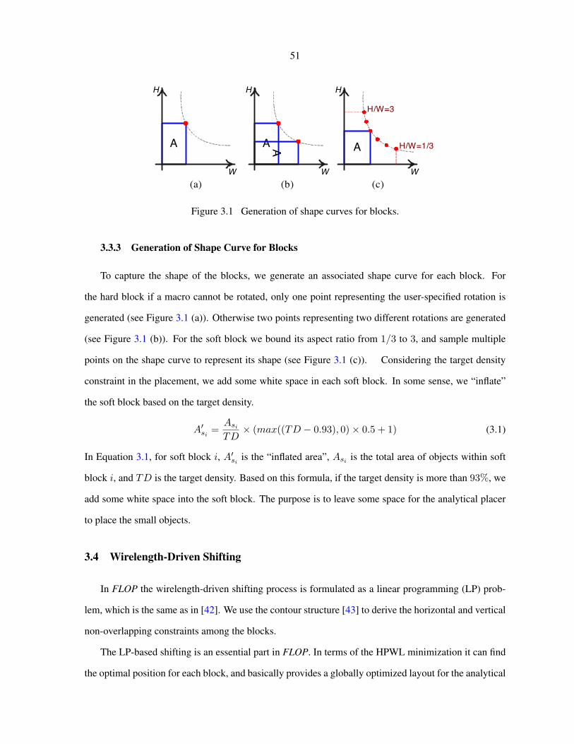
51
A
H
W
AA
H
W
A
H
W
H/W=3
H/W=1/3
(a) (b) (c)
Figure 3.1 Generation of shape curves for blocks.
3.3.3 Generation of Shape Curve for Blocks
To capture the shape of the blocks, we generate an associated shape curve for each block. For
the hard block if a macro cannot be rotated, only one point representing the user-specified rotation is
generated (see Figure 3.1 (a)). Otherwise two points representing two different rotations are generated
(see Figure 3.1 (b)). For the soft block we bound its aspect ratio from 1/3 to 3, and sample multiple
points on the shape curve to represent its shape (see Figure 3.1 (c)). Considering the target density
constraint in the placement, we add some white space in each soft block. In some sense, we “inflate”
the soft block based on the target density.
A′si=Asi
TD× (max((TD − 0.93), 0)× 0.5 + 1) (3.1)
In Equation 3.1, for soft block i, A′siis the “inflated area”, Asi is the total area of objects within soft
block i, and TD is the target density. Based on this formula, if the target density is more than 93%, we
add some white space into the soft block. The purpose is to leave some space for the analytical placer
to place the small objects.
3.4 Wirelength-Driven Shifting
In FLOP the wirelength-driven shifting process is formulated as a linear programming (LP) prob-
lem, which is the same as in [42]. We use the contour structure [43] to derive the horizontal and vertical
non-overlapping constraints among the blocks.
The LP-based shifting is an essential part in FLOP. In terms of the HPWL minimization it can find
the optimal position for each block, and basically provides a globally optimized layout for the analytical

52
placer. Since the LP-based shifting optimizes the HPWL at the floorplan level, it only ignores the local
nets among the small objects within each soft block. The smaller the soft block is, the less nets it
ignores, and the better the HPWL we will get at last. However, if the soft blocks become too small,
numerous nets will be considered in the shifting. This would slow down the whole algorithm. Because
of this, in the partition stopping criteria we set an area bound α, so that the soft blocks would not
become too small. On the other hand, we only need the shifting step to generate a globally good layout.
Regarding the local nets within the soft blocks, we believe the following analytical placer can handle
them very efficiently and effectively.
3.5 Incremental Placement
As mentioned before, the output of the wirelength-driven shifting step is a layout with legal, non-
overlapping locations for the big macros. These big macros are then fixed in place to prevent further
movement during any subsequent steps. But, there are multiple “soft blocks” in the layout, each con-
taining numerous “small objects”. These small objects are a combination of standard cells and small
macros. The floorplanning step assigns these small objects to the center of the corresponding soft block.
In this respect, the placement step has two key tasks: 1) Spread the small objects over the placement
region and obtain a final overlap free placement among all objects; 2) Use the initial locations of the
small objects as obtained by the shifting step.
To satisfy these two tasks, we use an efficient analytical incremental placement algorithm. The
incremental placement flow is as shown in Figure 3.2.
3.6 MMS Benchmarks
The only publicly available benchmarks for mixed-size designs are ISPD02 and ICCAD04 IBM-
MS [10, 46] that are derived from ISPD98 placement benchmarks. As pointed out in [40], these circuits
can no longer be representative of modern VLSI physical design. To continue driving the progress
of physical design for the academic community, two suites of placement benchmarks [40, 41] have
been released recently. They are directly derived from modern industrial ASICs design. Unfortunately,
however, in the original circuits most macros have been fixed due to the difficulty of handling movable

53
1: Phase 0: Physical and Netlist based clustering2: initial objects← number of small objects3: set locations of small objects to center of their soft blocks4: while number of clusters > target number of clusters do5: cluster netlist using Best-choice clustering [44]6: use physical locations of small objects in clustering score7: set cluster location← center of gravity of the objects within cluster8: end while9: end
10: Phase 1: Coarse global placement11: generate “fixing forces” for clusters based on their initial locations12: solve initial quadratic program (QP)13: repeat14: perform Cell Shifting [3] on coarse-grain clusters15: add spreading forces to QP formulation16: solve the quadratic program17: until placement is roughly even18: repeat19: perform Iterative Local Refinement [3] on coarse-grain clusters20: until placement is quite even21: uncluster movable macro-blocks22: legalize and fix movable macro-blocks23: end24: Phase 2: Refinement of fine-grain clusters25: while number of clusters < 0.5*number of small objects do26: uncluster netlist27: end while28: perform Iterative Local Refinement on fine-grain clusters29: end30: Phase 3: Refinement of flat netlist31: while number of clusters < number of small objects do32: uncluster netlist33: end while34: perform Iterative Local Refinement on flat netlist35: end36: Phase 4: Legalization and detailed placement37: Legalize the standard cells in the presence of fixed macros38: Perform detailed placement [45] to further improve wirelength39: end
Figure 3.2 Algorithm of analytical incremental placement.

54
macros for the existing placers. The authors in [8, 9] freed all fixed objects in ISPD06 benchmarks
and created new mixed-size placement circuits. But seven out of eight circuits do not have any fixed
I/O objects, which is not realistic in the real designs. In order to recover the complexities of modern
mixed-size designs, we modify the original ISPD05/06 benchmarks and derive the Modern Mixed-Size
(MMS) placement benchmarks (see Table 3.1).

55
Table 3.1 Statistics of Modern Mixed-Size placement benchmarks.
Circuit #Objects #Movable Objects #Standard Cells #Macros #Fixed I/O Objects #Net #Net Pins Target Density% λ
adaptec1 211447 210967 210904 63 480 221142 944053 100 70adaptec2 255023 254584 254457 127 439 266009 1069482 100 160adaptec3 451650 450985 450927 58 665 466758 1875039 100 650adaptec4 496054 494785 494716 69 1260 515951 1912420 100 460bigblue1 278164 277636 277604 32 528 284479 1144691 100 120bigblue2 557866 535741 534782 959 22125 577235 2122282 100 30bigblue3 1096812 1095583 1093034 2549 1229 1123170 3833218 100 470bigblue4 2177353 2169382 2169183 199 7970 2229886 8900078 100 550adaptec5 843128 842558 842482 76 570 867798 3493147 50 440newblue1 330474 330137 330073 64 337 338901 1244342 80 2000newblue2 441516 440264 436516 3748 1252 465219 1773855 90 190newblue3 494011 482884 482833 51 11127 552199 1929892 80 170newblue4 646139 642798 642717 81 3341 637051 2499178 50 400newblue5 1233058 1228268 1228177 91 4790 1284251 4957843 50 570newblue6 1255039 1248224 1248150 74 6815 1288443 5307594 80 650newblue7 2507954 2481533 2481372 161 26421 2636820 10104920 80 650
56
Essentially, we make the following changes on the original circuits.
I. Macros are freed from the original positions. In the GSRC Bookshelf format that the original
benchmarks use, both fixed macros and fixed I/O objects are treated as fixed objects. There is no extra
specification to differentiate them. So we have to distinguish them only based on the size differences.
Basically, if the area of one fixed object is more than λ× the average area of the whole circuit, we
will recognize it as a macro. Otherwise, it is a fixed I/O object. Because for each circuit the average
area is different, we need to use a different λ (see the last column in Table 3.1) to decide a reasonable
number and suitable threshold size for the macros. There is one exception: in both circuits bigblue2
and bigblue4, there is one macro that does not connect with any other objects. If this macro is freed, it
may cause some trouble for quadratic-based analytical placers. So we keep it fixed. Since this macro is
also very small compared with other macros, it would not affect circuit property.
II. The sizes of all I/O objects are set to zero. In MMS benchmarks there are two types of
I/Os: perimeter I/Os around the chip boundary and area-array I/Os spreading across the chip region.
Generally, the area-array I/Os are allowed to be overlapped with other movable objects in the design.
But existing placers treat all fixed I/Os as fixed objects, so that their algorithms internally do not allow
such overlaps during the legalization. Since the macros have already been freed in MMS benchmarks,
other placers should ignore the overlaps between fixed I/O objects and movable objects, and concentrate
on the legalization of movable objects. As we cannot change the code of other placers, one simple way
to enforce this is to set the sizes of all I/O objects to zero.
The target density constraints are the same as the original circuits. The same scoring function [41]
is used to get the scaled HPWL. But since the macros are movable in MMS, we need to modify the
script used in [41] to get the “scaled overflow factor”. The modification being: Any movable macro
that has a width or height greater than the bin dimension used for scaled overflow calculation, is now
treated as a fixed macro during scaled overflow calculation. Note that, this was the method employed
by the original script on newblue1, which is the only design that has big movable macros in the original
circuits. It is required to treat big movable macros as fixed, otherwise we will get an incorrect picture
of the placement density.
We have discussed the MMS benchmarks setup with the authors in [40, 41]. To keep the original
57
circuit properties as much as possible, the above changes are the best we can do without accessing the
original industrial data of the circuits. The MMS benchmarks are publicly available at [39].
3.7 Experimental Results
All experiments were performed on a Linux machine with AMD Opteron 2.6 GHz CPU and 8GB
memory. We use hMetis2.0 [47] as the partitioner and QSopt [48] as the LP solver. The seed of
hMetis2.0 is set to 5. Essentially, we set up four experiments.
I. To test the capability of handling the complexities in modern large-scale mixed-size placement,
we compare FLOP with five state-of-the-art mixed-size placers: APlace2, NTUplace3, mPL6, Capo10.5
and Kraftwerk on MMS benchmarks. Before the experiments, we contacted the developers of each
placer above, and they provided us their best-available binary for MMS benchmarks. In Table 3.2, for
the ISPD06 circuits (adaptec5 - newblue7) the reported HPWL is the scaled HPWL. FLOP is the default
mode of FLOP with all macros rotatable, and FLOP-NR restricts the rotation on every macro. APlace2
crashed on every circuit, so we do not show its results. For the default mode, FLOP generates 8%, 2%,
44% and 26% better HPWL compared with NTUplace3, mPL6, Capo10.5 and Kraftwerk, respectively.
About the runtime, FLOP is 6× and 3× faster than Capo10.5 and mPL6. Also FLOP achieves legal
solution on every circuit. Compared with FLOP-NR, FLOP generates 4% better HPWL by rotating the
macros.
II. To show the importance of respecting the initial positions of small objects in the incremental
placement step, we generate the results of FLOP-NI, which discards the such information and places
all small objects from scratch. As shown in Table 3.2, FLOP-NI produces 5% worse HPWL and 20%
slower than FLOP.
III. We compare FLOP with three leading macro placers, CG, MPT and XDP. Due to the IP issues,
we cannot get their binaries. But the authors sent us their benchmarks used in [9]. So the other placers’
results in Table 3.3 are cited from [9]. These benchmarks allow the rotation of macros, and do not
consider the target density. Also only one circuit has boundary I/Os, others do not have any I/Os at all.
As we can see, FLOP achieves 1%, 12%, 7% and 14% better HPWL compared with CG, MPT, XDP
and NTUplace3, respectively. We also use NTUplace3 to substitute the incremental placer in FLOP,
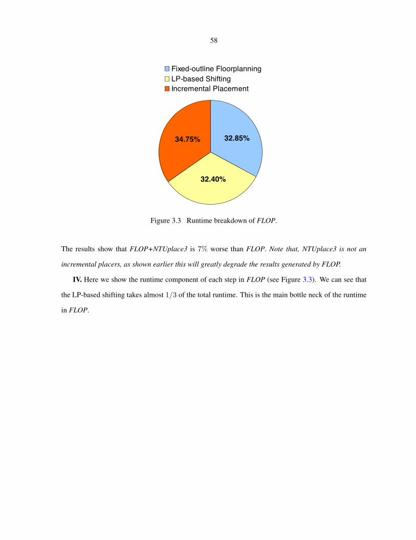
58
34.75%
32.40%
32.85%
Fixed-outline FloorplanningLP-based ShiftingIncremental Placement
Figure 3.3 Runtime breakdown of FLOP.
The results show that FLOP+NTUplace3 is 7% worse than FLOP. Note that, NTUplace3 is not an
incremental placers, as shown earlier this will greatly degrade the results generated by FLOP.
IV. Here we show the runtime component of each step in FLOP (see Figure 3.3). We can see that
the LP-based shifting takes almost 1/3 of the total runtime. This is the main bottle neck of the runtime
in FLOP.

59
Table 3.2 Comparison with mixed-size placers on MMS benchmarks (* compared with scaled HPWL),HPWL(×10e6).
Circuit NTUplace3[7] mPL6[6] Capo10.5[2] Kraftwerk[49] FLOP-NR FLOP-NI FLOPHPWL Time(s) HPWL Time(s) HPWL Time(s) HPWL Time(s) HPWL Time(s) HPWL Time(s) HPWL Time(s)
adaptec1 80.45 630 77.84 2404 84.77 5567 86.73 285 77.18 722 85.27 961 76.83 824adaptec2 136.46 1960 88.40 2870 92.61 7373 108.61 408 87.17 1219 86.72 1394 84.14 1192adaptec3 illegal – 180.64 5983 202.37 16973 272.76 773 182.21 1943 173.07 2394 175.99 2116adaptec4 177.23 1896 162.02 5971 202.38 17469 260.96 962 166.55 2398 175.67 2753 161.68 2427bigblue1 95.11 955 99.36 2829 112.58 8458 130.78 348 95.45 1776 98.91 2245 94.92 2007bigblue2 144.42 1661 144.37 12202 149.54 17647 abort – 150.66 2373 162.40 3830 153.02 3110bigblue3 illegal – 319.63 9548 583.37 69921 417.73 2369 372.79 7037 394.75 6959 346.24 5437bigblue4 764.72 8182 804.00 23868 915.73 109785 969.03 6000 807.53 13816 839.53 22788 777.84 19671
adaptec5* abort – 376.30 22636 565.88 23957 402.21 1653 381.83 5048 385.07 4067 357.83 3293newblue1* 60.73 875 66.93 3171 110.54 3133 76.22 481 73.36 1368 71.69 1302 67.97 1012newblue2* abort – 179.18 6044 303.25 8156 272.67 615 231.94 2646 190.50 2998 187.40 2414newblue3* abort – 415.86 17623 1282.19 73339 374.54 578 344.71 2336 355.07 3389 345.99 2757newblue4* abort – 277.69 9732 300.69 6589 291.45 1266 256.91 2575 268.46 3579 256.54 2455newblue5* abort – 515.49 24806 570.32 16548 503.13 2639 516.71 8801 536.38 11010 510.83 9163newblue6* abort – 482.44 13112 609.16 18076 651.34 2726 502.24 9450 506.99 11195 493.64 9563newblue7* abort – 1038.66 31680 1481.45 43386 illegal – 1113.07 18765 1101.07 26979 1078.18 25104
Norm 1.08 0.78 1.02 2.95 1.44 6.56 1.26 0.35 1.04 1.00 1.05 1.17 1 1
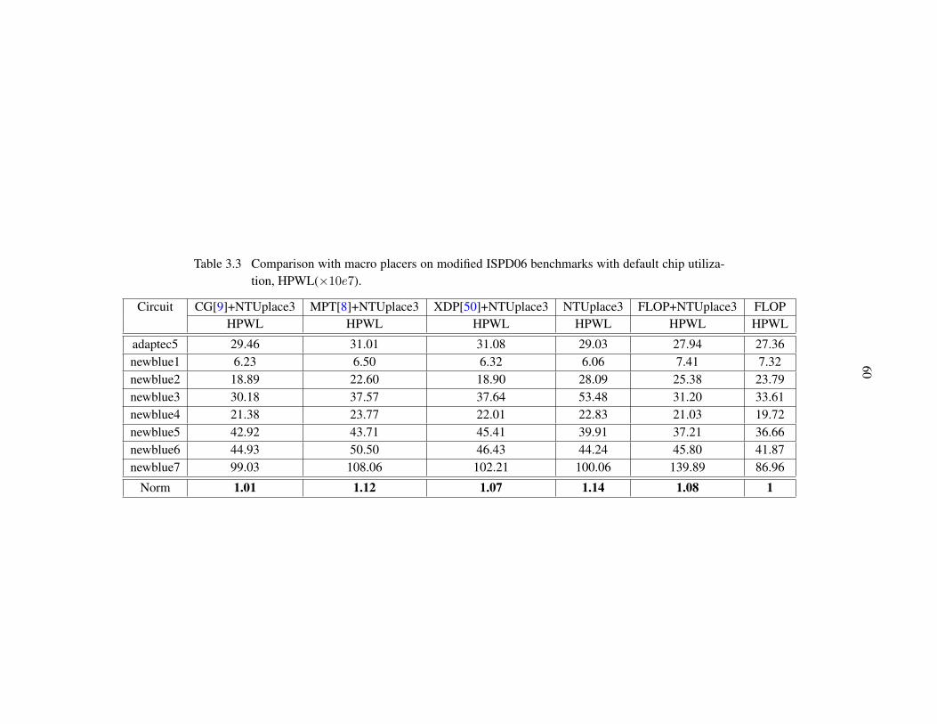
60
Table 3.3 Comparison with macro placers on modified ISPD06 benchmarks with default chip utiliza-tion, HPWL(×10e7).
Circuit CG[9]+NTUplace3 MPT[8]+NTUplace3 XDP[50]+NTUplace3 NTUplace3 FLOP+NTUplace3 FLOPHPWL HPWL HPWL HPWL HPWL HPWL
adaptec5 29.46 31.01 31.08 29.03 27.94 27.36newblue1 6.23 6.50 6.32 6.06 7.41 7.32newblue2 18.89 22.60 18.90 28.09 25.38 23.79newblue3 30.18 37.57 37.64 53.48 31.20 33.61newblue4 21.38 23.77 22.01 22.83 21.03 19.72newblue5 42.92 43.71 45.41 39.91 37.21 36.66newblue6 44.93 50.50 46.43 44.24 45.80 41.87newblue7 99.03 108.06 102.21 100.06 139.89 86.96
Norm 1.01 1.12 1.07 1.14 1.08 1
61
3.8 Conclusion
In this chapter, we presented a high-quality mixed-size placer FLOP. Compared with the state-
of-the-art mixed-size placers and leading macro placers, FLOP achieves the best HPWL, and easily
produces the overlap-free layout for every circuit.
We believe there is room to further improve the QoR of FLOP. First, we can use the min-cost
flow algorithm to substitute the linear programming formulation in order to speed up the shifting step.
Second, we observe that the partitioning takes around 80% of the total runtime in the floorplanning.
Thus a stand-alone clustering algorithm is needed in the block formation to cut down the problem size
before partitioning. This will definitely improve both the runtime and HPWL. Third, by enhancing
the floorplanning framework, FLOP can also be extended to handle other problems, e.g. mixed-size
placement with geometry constraints. All of the above three issues will be addressed in Chapter 6.

62
CHAPTER 4 Hypergraph Clustering for Wirelength-Driven Placement
Our first mission is to ask if they are safe.
— Maureen Blaha
4.1 Introduction
For modern VLSI designs, placement is the most critical stage in the physical synthesis flow. It has
significant impacts on timing, routing and even manufacturing. In the nanometer scale era, a circuit
typically contains millions of objects. It is extremely challenging for a modern placer to be reasonably
fast, yet still be able to produce good solutions. Clustering cuts down the problem size via combining
highly connected objects, so that the placers can perform more efficiently and effectively on a smaller
problem. It is an attractive solution to cope with the ever-increasing design complexity. Therefore, as
an essential approach to improve both the runtime and quality of result, various clustering algorithms
have been adopted in the state-of-the-art placement algorithms [7, 2, 51, 4, 6, 3, 52, 13].
4.1.1 Previous Work
Clustering is a traditional problem in VLSI Computer-Aided Design (CAD) area. The clustering
algorithms proposed long time ago were described in [53]. In the last several years, various new algo-
rithms were proposed to continue improving the clustering quality. In [54] Karypis et al. proposed edge
coarsening (EC) clustering. In EC objects are randomly visited. Each object is clustered with the most
highly-connected unvisited neighbor object. The connectivity between two objects is computed as the
total weight of all edges connecting them with hyperedges represented by a clique model. FirstChoice
(FC) clustering was developed in [34] and is very similar to EC. The only difference between them is
63
that for each object in FC, all of its neighbor objects are considered for clustering. FC has been used
in placers NTUplace3 [7] and Capo [2]. However, neither EC nor FC considers the impact of cluster
size on the clustering quality. Alpert et al. [55] and Chan et al. [56] improved EC and FC respectively,
by considering the area of clusters, i.e., clusters with smaller area are preferred to be generated. Cong
et al. [57] proposed an edge separability-based clustering (ESC). Unlike previous methods, ESC uses
edge separability to guide the clustering process. To explore global connectivity information, all edges
are ranked via a priority queue (PQ) based on the edge separability. Without violating the cluster size
limit, the two objects in the highest ranking edge are clustered. Hu et al. [58] developed fine granularity
(FG) clustering. The difference between FG and ESC is that for FG the order in the PQ is based on edge
contraction measured by a mutual contraction metric. FG has been used in placer mFAR [51]. Nam et
al. [59] proposed BestChoice (BC) clustering which has been widely used in the top-of-the-line placers
APlace [4], mPL6 [6], FastPlace3 [3], RQL [52] and FLOP [13]. Instead of ranking the edges, BC
maintains a PQ based on a pair of objects, i.e., each object and its best neighbor object. A score func-
tion considering both hyperedge weight and object area is derived to calculate the score between two
objects. For each object, the best neighbor object is the neighbor object with the highest score. The two
objects at the top of the PQ are clustered iteratively. But updating such a PQ is quite time-consuming.
Hence, the authors proposed a lazy-update technique to make a trade-off between the clustering runtime
and quality.
All of the above clustering algorithms either explicitly or implicitly transform a hyperedge into
a clique model, so that they can handle pair-wise clustering, i.e., cluster two objects at each time.
Recently, Li et al. [60] presented NetCluster (NC) that can handle hyperedges directly and cluster more
than two objects at one time. In NC, initial clusters are first generated by FM algorithm [61]. Then a
score is assigned to each net. The objects in the net with the highest score are clustered.
For all previous clustering algorithms, none of them specifically aims at improving the placement
quality. They proposed a variety of heuristics, e.g., different score functions, to measure the direct con-
nectivity among the objects, so that the most highly directly connected objects are clustered. Of course,
the benefit is a reduction of problem size. But, clustering such objects may not help the placer to pro-
duce better solution. This is because clustering forces some objects to stay together during placement,
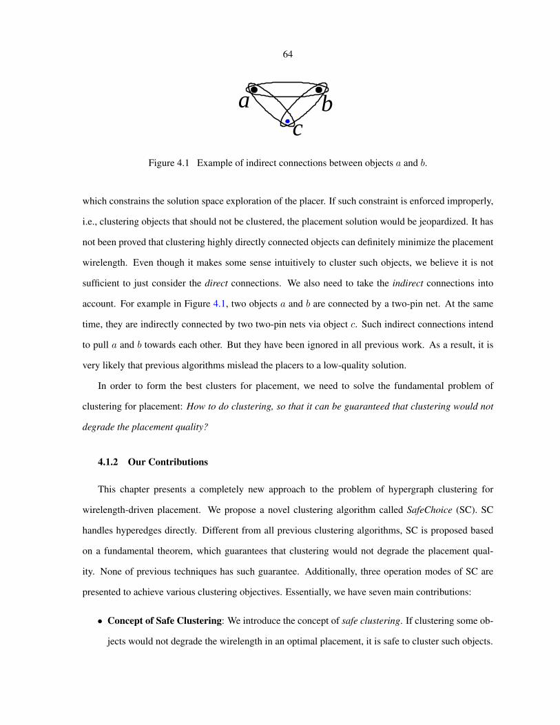
64
a bc
Figure 4.1 Example of indirect connections between objects a and b.
which constrains the solution space exploration of the placer. If such constraint is enforced improperly,
i.e., clustering objects that should not be clustered, the placement solution would be jeopardized. It has
not been proved that clustering highly directly connected objects can definitely minimize the placement
wirelength. Even though it makes some sense intuitively to cluster such objects, we believe it is not
sufficient to just consider the direct connections. We also need to take the indirect connections into
account. For example in Figure 4.1, two objects a and b are connected by a two-pin net. At the same
time, they are indirectly connected by two two-pin nets via object c. Such indirect connections intend
to pull a and b towards each other. But they have been ignored in all previous work. As a result, it is
very likely that previous algorithms mislead the placers to a low-quality solution.
In order to form the best clusters for placement, we need to solve the fundamental problem of
clustering for placement: How to do clustering, so that it can be guaranteed that clustering would not
degrade the placement quality?
4.1.2 Our Contributions
This chapter presents a completely new approach to the problem of hypergraph clustering for
wirelength-driven placement. We propose a novel clustering algorithm called SafeChoice (SC). SC
handles hyperedges directly. Different from all previous clustering algorithms, SC is proposed based
on a fundamental theorem, which guarantees that clustering would not degrade the placement qual-
ity. None of previous techniques has such guarantee. Additionally, three operation modes of SC are
presented to achieve various clustering objectives. Essentially, we have seven main contributions:
• Concept of Safe Clustering: We introduce the concept of safe clustering. If clustering some ob-
jects would not degrade the wirelength in an optimal placement, it is safe to cluster such objects.
65
• Safe Condition: Based on the concept of safe clustering, we derive the fundamental theorem —
safe condition for pair-wise clustering. We prove that if any two objects satisfy the safe condition,
clustering them would not degrade the wirelength.
• Selective Enumeration: To check the safe condition for pair-wise clustering, we propose selec-
tive enumeration. With such method, we can efficiently find out the safe clusters in a circuit.
• SafeChoice: We present SafeChoice algorithm that globally ranks potential clusters via a PQ
based on their safeness and area. Iteratively the cluster at the top of the PQ will be formed.
• Smart Stopping Criterion: A smart stopping criterion is proposed based on a simple heuristic.
So it can automatically stop clustering once generating more clusters would start to degrade the
placement wirelength. As far as we know, none of previous algorithms has such feature.
• Physical SafeChoice: We extend SafeChoice to do clustering if the physical locations of some
objects are given. In this way, SafeChoice can make use of such location information, e.g., an
initial placement or fixed I/O object locations, and thus produces even better clusters.
• SCPlace: To demonstrate the effectiveness of Physical SafeChoice, we propose a simple and
high-quality two-phase placement algorithm called SCPlace. SCPlace is simple in the sense that
it has only one clustering level and two placement phases. But, it produces significantly better
results than all other state-of-the-art placement algorithms.
We compare SC with three state-of-the-art clustering algorithms FC, BC and NC. The results show that
the clusters produced by SC consistently helps the placer to generate the best wirelength. Compared
with the state-of-the-art placement algorithms, SCPlace is able to generate the best HPWL.
The rest of this chapter is organized as follows. Section 4.2 describes the safe clustering. Section 4.3
introduces the algorithm of SafeChoice. Section 4.4 presents the Physical SafeChoice. Section 4.5
introduces the algorithm of SCPlace. Experimental results are presented in Section 4.6. Finally, this
chapter ends with a conclusion and the direction of future work.

66
4.2 Safe Clustering
In this section, we first introduce the concept of safe clustering. Then based on this concept we de-
rive the safe condition for pair-wise clustering. Finally we propose selective enumeration to practically
check the safe condition for any two objects in the circuit.
First of all, we introduce some notations used in the discussion. The original netlist is modeled by
a hypergraph G(V,E), where V is the set of vertices and E is the set of hyperedges. Given v ∈ V ,
Ev is the set of hyperedges incident to v, and Ev = E − Ev. Let P be the set of all possible legalized
placements of the vertices in V . The wirelength is measured by weighted HPWL.
4.2.1 Concept of Safe Clustering
The concept of safe clustering is defined as follows.
Definition 1. Safe Clustering: For a set of vertices Vc ⊆ V (|Vc| ≥ 2), if the optimal wirelength of the
netlist generated by clustering Vc is the same as the optimal wirelength of the original netlist, then it is
safe to cluster the vertices in Vc.
The placement problem is NP-hard. In practice we cannot find the optimal wirelength for a real
circuit. So we present a more practical definition below.
Definition 2. Safe Clustering?: ∀p ∈ P , if a set of vertices Vc ⊆ V (|Vc| ≥ 2) can be moved to the
same location without increasing the wirelength, then it is safe to cluster the vertices in Vc.
Definition 2 is established based an assumption that the area of every vertex in Vc is zero, so that we
can move them in a legalized placement and ignore the overlap issue. In other words, we only consider
clustering zero-area objects. Definition 2 shows that when safe clustering is performed on any legalized
(zero-overlap) placement p, it does not increase the total wirelength of p. But, the clustering algorithm
is not a placement algorithm and thus does not specify how any overlap incurred by the clustering is
to be removed. Therefore, we assume that the clusters are small enough, i.e., zero area, compared to
the total area of place-able objects in the clustered netlist, such that any wirelength increase incurred by
any displacement needed to remove overlap incurred by the clustering does not exceed the wirelength
decrease induced by the clustering. This assumption is reasonable, even though there is no zero-area

67
object in the real circuits. This is because for a typical clustering ratio 1, the size of each cluster is
always much smaller than the total area of objects in the circuit. Note that, however, such assumption
may not be applicable when some complex floorplan geometry is presented, e.g., when a big cluster
is placed in a narrow channel between two big fixed objects. In this case, the displacement needed to
remove overlap incurred by the clustering may be quite big.
As you can see, Definition 2 is stronger than Definition 1. If Vc is safe for clustering based on
Definition 2, it is also safe under Definition 1. In the rest of this chapter, we employ Definition 2
for discussion. Based on Definition 2, we derive the definitions for horizontally and vertically safe
clustering as follows.
Definition 3. Horizontally/Vertically Safe Clustering: ∀p ∈ P , if a set of vertices Vc ⊆ V (|Vc| ≥ 2)
can be horizontally/vertically moved to the same x/y coordinate without increasing the wirelength in
x/y direction, then it is horizontally/vertically safe to cluster the vertices in Vc.
Now we show that if vertices in Vc are both horizontally and vertically safe for clustering, then
it is safe to cluster them under Definition 2. Given any initial placement p ∈ P , firstly we move
those vertices horizontally to the same x coordinate. Secondly, we move them vertically to the same
y coordinate. Consequently, the vertices in Vc are moved to the same location. Based on Definition 3
the wirelength would not increase during the movements. So it is safe to cluster the vertices in Vc by
Definition 2.
In the remaining part of Section 4.2, we consider only x direction and horizontally safe cluster-
ing. Analogically, the theoretical proof and mathematical derivation for y direction and vertical safe
clustering can be done in a similar way.
4.2.2 Safe Condition for Pair-Wise Clustering
From Definition 2 we derive a condition to mathematically determine whether it is safe to cluster
the vertices in Vc. Firstly, we define two key functions for the derivation. For the sake of simplicity, we
always assume Vc contains only two vertices a and b (i.e., Vc = {a, b}), and a is on the left of b.
1The clustering ratio is defined as the ratio of the number of objects in the clustered circuit to the number of objects in theoriginal circuit.

68
Definition 4. Wirelength Gradient Function: Given a placement p ∈ P and a hyperedge e ∈ E, we
define
∆a(p, e) : Gradient function of wirelength of e, if a is moving towards b.
∆b(p, e) : Gradient function of wirelength of e, if b is moving towards a.
Let we(we ≥ 0) be the weight of e. From Definition 4 we have
∆a(p, e) =
we if a is the rightmost vertex of e
−we if a is the only leftmost vertex of e
0 otherwise
∆b(p, e) =
we if b is the leftmost vertex of e
−we if b is the only rightmost vertex of e
0 otherwise
Considering a is moving towards b in p, if ∆a(p, e) > 0, it means the wirelength of e will increase; if
∆a(p, e) < 0, then the wirelength of e will decrease; otherwise the wirelength of e will not change.
Definition 5. Total wirelength Gradient Function: Given a placement p ∈ P and Vc = {a, b}, we
define
Fab(p) = min(∑e∈Ea
∆a(p, e),∑e∈Eb
∆b(p, e))
In p if both a and bmove towards each other,Fab(p) first calculates the total wirelength change of all
hyperedges for moving a and b, respectively. Then it returns the one with smaller change. For example,
if Fab(p) =∑
e∈Ea∆a(p, e) ≤ 0, it means moving a towards b would not increase the total wirelength;
if Fab(p) > 0, then moving either a or b towards each other would increase the total wirelength. Next,
we use this function to derive the safe condition for a and b.
Theorem 1. Safe Condition for Vc = {a, b}
It is safe to cluster a and b if ∀p ∈ P,Fab(p) ≤ 0
Proof. Given an initial placement p0 ∈ P with total wirelength l0. Because ∀p ∈ P,Fab(p) ≤ 0,
we have Fab(p0) ≤ 0. Suppose Fab(p0) =∑
e∈Ea∆a(p0, e) ≤ 0. This means by moving a a small
distance towards b, the total wirelength of all hyperedges would not increase. After such movement, we

69
get another placement p1 with total wirelength l1, where l0 ≥ l1. For p1 we still have Fab(p1) ≤ 0.
Suppose this time Fab(p1) =∑
e∈Eb∆b(p1, e) ≤ 0. This means moving b a small distance towards a
would not increase the total wirelength. Again, after such movement, we get another placement p2 with
total wirelength l2, where l1 ≥ l2. We keep moving either a or b towards each other until they reach the
same location. Suppose the final total wirelength is ln. Because after each movement we always have
Fab(p) ≤ 0, which means the total wirelength would not increase, eventually we have l0 ≥ ln.
As a result, given any initial placement p0 we can gradually move a and b to the same location
without increasing the wirelength. So based on Definition 2, it is safe to cluster vertices a and b.
4.2.3 Selective Enumeration
To check whether it is safe to cluster a and b, Theorem 1 shows that we need to generate all place-
ments in P . To do so, we have to enumerate all possible positions for all vertices in V . Apparently this
is not a practical approach. In this section, we show that in order to check Theorem 1, it is sufficient to
consider only a small subset of placements. Selective enumeration technique is proposed to enumerate
such necessary placements.
Selective enumeration is motivated by the following principle: Given two placements p1, p2 ∈ P , if
we know Fab(p1) ≤ Fab(p2), then p1 can be ignored in the enumeration. This is because Theorem 1
shows that the safe condition is only determined by the placement with the maximum Fab(p) value. So
the basic idea of selective enumeration is to find out the relationship of Fab(p) values among different
placements, so that in the enumeration process we can ignore the placements with smaller or equal
Fab(p) values. Placements in P are generated by different positions of different vertices. Our goal is to
identify some vertices in V , such that some or even all of their possible positions can be ignored.
We first classify the vertices in V into two categories Vab and Vab (Vab ∪ Vab ∪ {a, b} = V ). Then
we discuss the enumeration of their positions separately. ∀v ∈ V , xv denotes the x coordinate of v.
1. Vab: vertices connecting with neither a nor b.
2. Vab: vertices connecting with at least one of a and b.
Lemma 1. Given a placement p ∈ P , by moving vertex v ∈ Vab to any other position, another place-
ment p′ ∈ P is generated. We have Fab(p) = Fab(p′).

70
Proof. Since ∀v ∈ Vab, v connects with neither a nor b, changing the position of v would not change
the leftmost or rightmost vertex of any hyperedge connecting with a or b. Therefore,
∀e ∈ Ea, ∆a(p, e) = ∆a(p′, e)
∀e ∈ Eb, ∆b(p, e) = ∆b(p′, e)
Thus, Fab(p) = Fab(p′).
Based on Lemma 1, in the enumeration we can simply ignore all vertices in Vab.
Lemma 2. Given a placement p ∈ P , vertex v ∈ Vab and xv = k1. After moving v to xv = k2, another
placement p′ ∈ P is generated. We have Fab(p) = Fab(p′) if any one of the following conditions is
satisfied: (1) k1 ≤ xa and k2 ≤ xa; (2) k1 ≥ xb and k2 ≥ xb; (3) xa < k1 < xb and xa < k2 < xb.
Proof. Suppose condition (1) holds, i.e., v is on the left of a in both p and p′. ∀e ∈ Ev, we consider
two2 possible values of ∆a(p, e):
• ∆a(p, e) = we
This means a is the rightmost vertex of e in p. After moving v to k2, because k2 ≤ xa, a is still
the rightmost vertex of e in p′. Thus, ∆a(p′, e) = we = ∆a(p, e).
• ∆a(p, e) = 0
This means a is neither the only leftmost nor the rightmost vertex of e in p. After moving v to k2,
because k2 ≤ xa, v is still on the left of a in p′. Thus, ∆a(p′, e) = 0 = ∆a(p, e).
So ∀e ∈ Ev, ∆a(p, e) = ∆a(p′, e). Similarly we have ∀e ∈ Ev, ∆b(p, e) = ∆b(p′, e). Therefore,
∀e ∈ Ea,∆a(p, e) = ∆a(p′, e)
∀e ∈ Eb,∆b(p, e) = ∆b(p′, e)
Thus, Fab(p) = Fab(p′). Analogically, the cases for conditions (2) and (3) can be proved as well.
Lemma 2 shows that ∀v ∈ Vab, instead of enumerating all possible positions, we only need to
consider three possibilities: (1) v is on the left of a (xv ≤ xa); (2) v is on the right of b (xv ≥ xb); (3) v
is between a and b (xa < xv < xb).2Because v is on the left of a, a would not be the only leftmost vertex of e. Thus, ∆a(p, e) 6= −we.
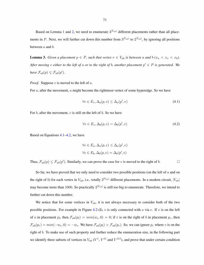
71
Based on Lemma 1 and 2, we need to enumerate 3|Vab| different placements rather than all place-
ments in P . Next, we will further cut down this number from 3|Vab| to 2|Vab|, by ignoring all positions
between a and b.
Lemma 3. Given a placement p ∈ P , such that vertex v ∈ Vab is between a and b (xa < xv < xb).
After moving v either to the left of a or to the right of b, another placement p′ ∈ P is generated. We
have Fab(p) ≤ Fab(p′).
Proof. Suppose v is moved to the left of a.
For a, after the movement, a might become the rightmost vertex of some hyperedge. So we have
∀e ∈ Ev,∆a(p, e) ≤ ∆a(p′, e) (4.1)
For b, after the movement, v is still on the left of b. So we have
∀e ∈ Ev,∆b(p, e) = ∆b(p′, e) (4.2)
Based on Equations 4.1–4.2, we have
∀e ∈ Ea,∆a(p, e) ≤ ∆a(p′, e)
∀e ∈ Eb,∆b(p, e) = ∆b(p′, e)
Thus, Fab(p) ≤ Fab(p′). Similarly, we can prove the case for v is moved to the right of b.
So far, we have proved that we only need to consider two possible positions (on the left of a and on
the right of b) for each vertex in Vab, i.e., totally 2|Vab| different placements. In a modern circuit, |Vab|
may become more than 1000. So practically 2|Vab| is still too big to enumerate. Therefore, we intend to
further cut down this number.
We notice that for some vertices in Vab, it is not always necessary to consider both of the two
possible positions. For example in Figure 4.2-(I), v is only connected with a via e. If v is on the left
of a in placement pl, then Fab(pl) = min(we, 0) = 0; if v is on the right of b in placement pr, then
Fab(pr) = min(−we, 0) = −we. We have Fab(pl) > Fab(pr). So, we can ignore pr where v is on the
right of b. To make use of such property and further reduce the enumeration size, in the following part
we identify three subsets of vertices in Vab (V I , V II and V III ), and prove that under certain condition

72
a b
ve
( I )
a b
ve
( II )
a b
ve
( III )
u
Figure 4.2 Simple examples of vertices that can be fixed.
the positions of those vertices can be fixed in the enumeration. Let Na denote the set of vertices sharing
at least one hyperedge with vertex a, and Na = V −Na. Similarly, we can define Nb and N b.
I. V I = Na ∩N b ( e.g., in Figure 4.2-(I) vertex v ∈ V I )
II. V II = Na ∩Nb ( e.g., in Figure 4.2-(II) vertex v ∈ V II )
III. V III = {v|v ∈ Vab s.t. (Ev ∩ (Ea ∪ Eb)) ⊂ (Ea ∩ Eb)} ( e.g., in Figure 4.2-(III) vertices
v, u ∈ V III )
Lemma 4. Given a placement p ∈ P , such that vertex v ∈ V I is on the left of a. After moving v to the
right of b, another placement p′ ∈ P is generated. We have Fab(p) ≥ Fab(p′).
Proof. Let Ev∩ab = Ev ∩ (Ea ∪ Eb).
• In placement p, ∀e ∈ Ev∩ab, we consider two cases:
– ∃ vertex c ∈ e(c 6= a, c 6= v), s.t. xc ≥ xb
Because xv ≤ xa and xc ≥ xb, xv ≤ xa ≤ xc. a is neither the only leftmost nor the
rightmost vertex of e. So ∆a(p, e) = 0.
– 6 ∃ vertex c ∈ e(c 6= a, c 6= v), s.t. xc ≥ xb
Because xv ≤ xa and no other vertices in e are on the right of b, a is the rightmost vertex
of e. So ∆a(p, e) = we.
Thus, ∀e ∈ Ev∩ab,∆a(p, e) ≥ 0.
• In placement p′, ∀e ∈ Ev∩ab, we consider two cases:
73
– ∃ vertex c ∈ e(c 6= a, c 6= v), s.t. xc ≤ xa
Because x′v ≥ xb and xc ≤ xa, xc ≤ xa ≤ x′v. a is neither the only leftmost nor the
rightmost vertex of e. So ∆a(p′, e) = 0.
– 6 ∃ vertex c ∈ e(c 6= a, c 6= v), s.t. xc ≤ xa
Because x′v ≥ xb and no other vertices in e are on the left of a, a is the only leftmost vertex
of e. So ∆a(p, e) = −we.
Thus, ∀e ∈ Ev∩ab,∆a(p′, e) ≤ 0.
So ∀e ∈ Ev∩ab,∆a(p, e) ≥ ∆a(p′, e). Also ∀v ∈ V I , v does not connect with b, so ∀e ∈ Ev∩ab,∆b(p, e) =
∆b(p′, e). Therefore,
∀e ∈ Ea,∆a(p, e) ≥ ∆a(p′, e)
∀e ∈ Eb,∆b(p, e) = ∆b(p′, e)
Thus, Fab(p) ≥ Fab(p′).
From Lemma 4, ∀v ∈ V I we can fix v on the left of a. As V II is symmetrical with V I , similarly we
can prove that ∀v ∈ V II we can fix v on the right of b.
Lemma 5. Given a placement p ∈ P , such that vertex v ∈ V III is on the left of a, vertex u ∈ V III is
on the right of b, and Ev ∩ (Ea ∪ Eb) = Eu ∩ (Ea ∪ Eb). After moving either one or both of them to
another position, i.e., moving v to the right of b and u to the left of a, another placement p′ is generated.
We have Fab(p) ≥ Fab(p′).
Proof. Let Ev−u = Ev ∩ (Ea ∪ Eb) = Eu ∩ (Ea ∪ Eb). We consider all three possible movements of
v and u.
• v moved to the right of b, u did not move
In placement p′, ∀e ∈ Ev−u we consider two cases:
– ∃ vertex c ∈ e(c 6= a), s.t. xc ≤ xa
In this case, a is neither the only leftmost nor the rightmost vertex in e, and b is neither the
leftmost nor the only rightmost vertex in e. So ∆a(p′, e) = 0, ∆b(p′, e) = 0.

74
– 6 ∃ vertex c ∈ e(c 6= a), s.t. xc ≤ xa
In this case, a is the only leftmost vertex in e, and b is neither the leftmost nor the only
rightmost vertex in e. So ∆a(p′, e) = −we, ∆b(p′, e) = 0.
• u moved to the left of a, v did not move
In placement p′, ∀e ∈ Ev−u we consider two cases:
– ∃ vertex c ∈ e(c 6= b), s.t. xc ≥ xb
In this case, a is neither the only leftmost nor the rightmost vertex in e, and b is neither the
leftmost nor the only rightmost vertex in e. So ∆a(p′, e) = 0, ∆b(p′, e) = 0.
– 6 ∃ vertex c ∈ e(c 6= b), s.t. xc ≥ xb
In this case, b is the only rightmost vertex in e, and a is neither the only leftmost nor the
rightmost vertex in e. So ∆a(p′, e) = 0, ∆b(p′, e) = −we.
• v moved to the right of b, u moved to the left of a
In this case, a is neither the only leftmost nor the rightmost vertex in e, and b is neither the
leftmost nor the only rightmost vertex in e. So ∀e ∈ Ev−u, ∆a(p′, e) = 0, ∆b(p′, e) = 0.
For all of the above cases, ∆a(p′, e) ≤ 0 and ∆b(p′, e) ≤ 0. In placement p, ∀e ∈ Ev−u because a is
neither the only leftmost nor the rightmost vertex in e, and b is neither the leftmost nor the only rightmost
vertex in e, we have ∆a(p, e) = ∆b(p, e) = 0. As a result, we have ∀e ∈ Ev−u, ∆a(p, e) ≥ ∆a(p′, e),
∆b(p, e) ≥ ∆b(p′, e), Therefore,
∀e ∈ Ea,∆a(p, e) ≥ ∆a(p′, e)
∀e ∈ Eb,∆b(p, e) ≥ ∆b(p′, e)
Thus, Fab(p) ≥ Fab(p′).
Lemma 5 shows that if ∃v, u ∈ V III and Ev ∩ (Ea ∪ Eb) = Eu ∩ (Ea ∪ Eb), then we can fix v to
the left of a and u to the right of b.
In all, we have identified three subsets of vertices in Vab. If certain condition is satisfied, those
vertices can be fixed in the enumeration. Note that those three subsets may not include all vertices that
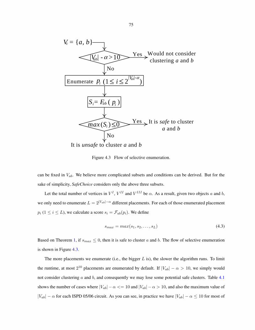
75
V = {a, b}
|V | - >10abYes Would not consider
clustering a and b
No
Enumerate
No
Yes It is safe to cluster a and b
It is unsafe to cluster a and b
c
α
pi (1 i )≤≤ 2 ab|V |- α
S = F ( p )i ab i
(S ) 0max ≤i
Figure 4.3 Flow of selective enumeration.
can be fixed in Vab. We believe more complicated subsets and conditions can be derived. But for the
sake of simplicity, SafeChoice considers only the above three subsets.
Let the total number of vertices in V I , V II and V III be α. As a result, given two objects a and b,
we only need to enumerate L = 2|Vab|−α different placements. For each of those enumerated placement
pi (1 ≤ i ≤ L), we calculate a score si = Fab(pi). We define
smax = max(s1, s2, . . . , sL) (4.3)
Based on Theorem 1, if smax ≤ 0, then it is safe to cluster a and b. The flow of selective enumeration
is shown in Figure 4.3.
The more placements we enumerate (i.e., the bigger L is), the slower the algorithm runs. To limit
the runtime, at most 210 placements are enumerated by default. If |Vab| − α > 10, we simply would
not consider clustering a and b, and consequently we may lose some potential safe clusters. Table 4.1
shows the number of cases where |Vab|−α <= 10 and |Vab|−α > 10, and also the maximum value of
|Vab| − α for each ISPD 05/06 circuit. As you can see, in practice we have |Vab| − α ≤ 10 for most of

76
Table 4.1 Profile of selective enumeration for each circuit.
Circuit Number of Cases Number of Cases Maximum|Vab| − α <= 10 (%) |Vab| − α > 10 (%) |Vab| − α
adaptec1 3079149 (94%) 205937 (6%) 78adaptec2 2834333 (92%) 252967 (8%) 110adaptec3 5568171 (90%) 591043 (10%) 191adaptec4 6362256 (93%) 448166 (7%) 110bigblue1 3677691 (94%) 218500 (6%) 154bigblue2 6941283 (95%) 351816 (5%) 1582bigblue3 12136725 (95%) 592998 (5%) 205bigblue4 22954456 (92%) 2104452 (8%) 1102adaptec5 9935184 (90%) 1058753 (10%) 278newblue1 4610210 (97%) 159220 (3%) 608newblue2 4058091 (98%) 73838 (2%) 144newblue3 6758853 (93%) 489111 (7%) 1016newblue4 9215574 (95%) 530334 (5%) 331newblue5 12046236 (94%) 744213 (6%) 372newblue6 15996670 (91%) 1527619 (9%) 1316newblue7 26414433 (94%) 1700947 (6%) 1151
the pairs (i.e., more than 90% of the pairs). Even if the unconsidered pairs are all safe, we would only
lose a very small portion of safe clusters.
4.3 Algorithm of SafeChoice
In the previous section, we have described a practical method of checking the safe condition for
pair-wise clustering. As shown in Definition 3, the safe condition has to be checked both horizontally
and vertically. However, without considering fixed vertices, e.g., I/O objects, if vertices in Vc are hori-
zontally safe for clustering, then they are always vertically safe for clustering as well. This is because a
vertical movement in a placement p is the same as a horizontal movement in another placement obtained
by rotating p by 90◦. If a set of vertices is horizontally safe for clustering, it is also vertically safe for
clustering, which means it is sufficient to check the safe condition only in x direction. Therefore, in
this section we ignore the fixed objects by treating them the same as movable ones, apply selective enu-
meration in a PQ-based algorithm flow and propose SafeChoice algorithm. To satisfy various clustering
objectives, we present three operation modes for SafeChoice.
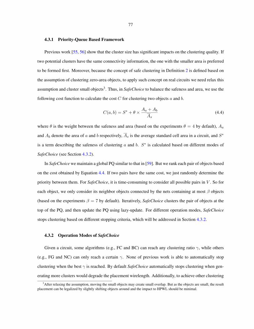
77
4.3.1 Priority-Queue Based Framework
Previous work [55, 56] show that the cluster size has significant impacts on the clustering quality. If
two potential clusters have the same connectivity information, the one with the smaller area is preferred
to be formed first. Moreover, because the concept of safe clustering in Definition 2 is defined based on
the assumption of clustering zero-area objects, to apply such concept on real circuits we need relax this
assumption and cluster small objects3. Thus, in SafeChoice to balance the safeness and area, we use the
following cost function to calculate the cost C for clustering two objects a and b.
C(a, b) = S∗ + θ × Aa +Ab
As(4.4)
where θ is the weight between the safeness and area (based on the experiments θ = 4 by default), Aa
and Ab denote the area of a and b respectively, As is the average standard cell area in a circuit, and S∗
is a term describing the safeness of clustering a and b. S∗ is calculated based on different modes of
SafeChoice (see Section 4.3.2).
In SafeChoice we maintain a global PQ similar to that in [59]. But we rank each pair of objects based
on the cost obtained by Equation 4.4. If two pairs have the same cost, we just randomly determine the
priority between them. For SafeChoice, it is time-consuming to consider all possible pairs in V . So for
each object, we only consider its neighbor objects connected by the nets containing at most β objects
(based on the experiments β = 7 by default). Iteratively, SafeChoice clusters the pair of objects at the
top of the PQ, and then update the PQ using lazy-update. For different operation modes, SafeChoice
stops clustering based on different stopping criteria, which will be addressed in Section 4.3.2.
4.3.2 Operation Modes of SafeChoice
Given a circuit, some algorithms (e.g., FC and BC) can reach any clustering ratio γ, while others
(e.g., FG and NC) can only reach a certain γ. None of previous work is able to automatically stop
clustering when the best γ is reached. By default SafeChoice automatically stops clustering when gen-
erating more clusters would degrade the placement wirelength. Additionally, to achieve other clustering3After relaxing the assumption, moving the small objects may create small overlap. But as the objects are small, the result
placement can be legalized by slightly shifting objects around and the impact to HPWL should be minimal.
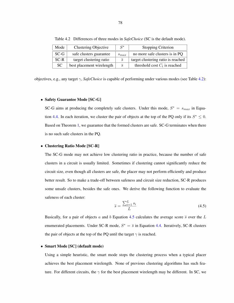
78
Table 4.2 Differences of three modes in SafeChoice (SC is the default mode).
Mode Clustering Objective S∗ Stopping Criterion
SC-G safe clusters guarantee smax no more safe clusters is in PQSC-R target clustering ratio s target clustering ratio is reached
SC best placement wirelength s threshold cost Ct is reached
objectives, e.g., any target γ, SafeChoice is capable of performing under various modes (see Table 4.2):
• Safety Guarantee Mode [SC-G]
SC-G aims at producing the completely safe clusters. Under this mode, S∗ = smax in Equa-
tion 4.4. In each iteration, we cluster the pair of objects at the top of the PQ only if its S∗ ≤ 0.
Based on Theorem 1, we guarantee that the formed clusters are safe. SC-G terminates when there
is no such safe clusters in the PQ.
• Clustering Ratio Mode [SC-R]
The SC-G mode may not achieve low clustering ratio in practice, because the number of safe
clusters in a circuit is usually limited. Sometimes if clustering cannot significantly reduce the
circuit size, even though all clusters are safe, the placer may not perform efficiently and produce
better result. So to make a trade-off between safeness and circuit size reduction, SC-R produces
some unsafe clusters, besides the safe ones. We derive the following function to evaluate the
safeness of each cluster:
s =∑L
i=1 siL
(4.5)
Basically, for a pair of objects a and b Equation 4.5 calculates the average score s over the L
enumerated placements. Under SC-R mode, S∗ = s in Equation 4.4. Iteratively, SC-R clusters
the pair of objects at the top of the PQ until the target γ is reached.
• Smart Mode [SC] (default mode)
Using a simple heuristic, the smart mode stops the clustering process when a typical placer
achieves the best placement wirelength. None of previous clustering algorithms has such fea-
ture. For different circuits, the γ for the best placement wirelength may be different. In SC, we

79
set a threshold cost Ct, and use the same cost function as in SC-R. During the clustering pro-
cess, SC would not terminate until the cost reaches Ct. Based on the experimental results, we set
Ct = 21 by default. With this simple heuristic, SC is able to automatically stop when generating
more clusters starts to degrade the placement wirelength.
4.4 Physical SafeChoice
In this section, we extend SafeChoice to do clustering while considering the object physical loca-
tions, i.e., physical clustering.
Compared with non-physical clustering algorithms, physical clustering is to do clustering based on
both the netlist connectivity information and the object physical locations. Such physical locations can
be obtained from an initial placement or existing fixed objects. It has been shown in [51, 3, 62, 52]
that the physical clustering can significantly improve the clustering quality. For SafeChoice, it is very
natural to be extended to physical clustering. This is because SafeChoice applies selective enumeration
to enumerate different placements. If an initial placement is given, many more placements can be
ignored in the enumeration. This simplifies the enumeration process by pruning away the placements
that would not be possibly generated.
In the following subsections, we first introduce the safe condition for Physical SafeChoice. After
that, we present how to further reduce the enumeration size based on the given physical information.
Finally, we show the corresponding changes of cost functions in different modes of Physical SafeChoice.
4.4.1 Safe Condition for Physical SafeChoice
Because in Physical SafeChoice the fixed objects are taken into account, horizontally safe may
not always imply vertically safe. Therefore, we need to consider the safe condition for both x and y
directions in Physical SafeChoice.
Definitions 4 and 5 are defined for x direction. But they can be easily extended to y direction. Based
on Theorem 1, we present the safe condition for Physical SafeChoice as follows.
Theorem 2. Safe Condition for Vc = {a, b} in Physical SafeChoice
It is safe to cluster a and b, if ∀p ∈ P,Fxab(p) ≤ 0 and Fyab(p) ≤ 0
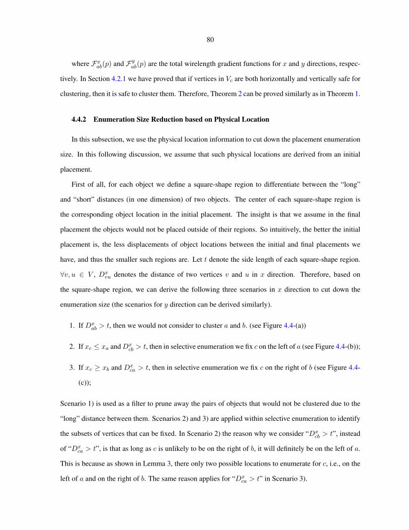
80
where Fxab(p) and Fyab(p) are the total wirelength gradient functions for x and y directions, respec-
tively. In Section 4.2.1 we have proved that if vertices in Vc are both horizontally and vertically safe for
clustering, then it is safe to cluster them. Therefore, Theorem 2 can be proved similarly as in Theorem 1.
4.4.2 Enumeration Size Reduction based on Physical Location
In this subsection, we use the physical location information to cut down the placement enumeration
size. In this following discussion, we assume that such physical locations are derived from an initial
placement.
First of all, for each object we define a square-shape region to differentiate between the “long”
and “short” distances (in one dimension) of two objects. The center of each square-shape region is
the corresponding object location in the initial placement. The insight is that we assume in the final
placement the objects would not be placed outside of their regions. So intuitively, the better the initial
placement is, the less displacements of object locations between the initial and final placements we
have, and thus the smaller such regions are. Let t denote the side length of each square-shape region.
∀v, u ∈ V , Dxvu denotes the distance of two vertices v and u in x direction. Therefore, based on
the square-shape region, we can derive the following three scenarios in x direction to cut down the
enumeration size (the scenarios for y direction can be derived similarly).
1. If Dxab > t, then we would not consider to cluster a and b. (see Figure 4.4-(a))
2. If xc ≤ xa andDxcb > t, then in selective enumeration we fix c on the left of a (see Figure 4.4-(b));
3. If xc ≥ xb and Dxca > t, then in selective enumeration we fix c on the right of b (see Figure 4.4-
(c));
Scenario 1) is used as a filter to prune away the pairs of objects that would not be clustered due to the
“long” distance between them. Scenarios 2) and 3) are applied within selective enumeration to identify
the subsets of vertices that can be fixed. In Scenario 2) the reason why we consider “Dxcb > t”, instead
of “Dxca > t”, is that as long as c is unlikely to be on the right of b, it will definitely be on the left of a.
This is because as shown in Lemma 3, there only two possible locations to enumerate for c, i.e., on the
left of a and on the right of b. The same reason applies for “Dxca > t” in Scenario 3).
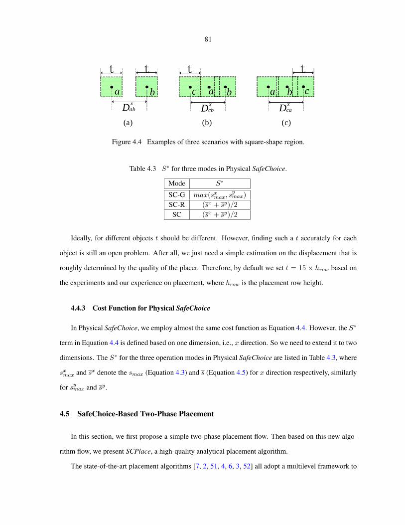
81
(a)
t t
Dabx
Dcbx
t
Dcax
t
(b) (c)
a b c a b a b c
Figure 4.4 Examples of three scenarios with square-shape region.
Table 4.3 S∗ for three modes in Physical SafeChoice.
Mode S∗
SC-G max(sxmax, symax)
SC-R (sx + sy)/2SC (sx + sy)/2
Ideally, for different objects t should be different. However, finding such a t accurately for each
object is still an open problem. After all, we just need a simple estimation on the displacement that is
roughly determined by the quality of the placer. Therefore, by default we set t = 15 × hrow based on
the experiments and our experience on placement, where hrow is the placement row height.
4.4.3 Cost Function for Physical SafeChoice
In Physical SafeChoice, we employ almost the same cost function as Equation 4.4. However, the S∗
term in Equation 4.4 is defined based on one dimension, i.e., x direction. So we need to extend it to two
dimensions. The S∗ for the three operation modes in Physical SafeChoice are listed in Table 4.3, where
sxmax and sx denote the smax (Equation 4.3) and s (Equation 4.5) for x direction respectively, similarly
for symax and sy.
4.5 SafeChoice-Based Two-Phase Placement
In this section, we first propose a simple two-phase placement flow. Then based on this new algo-
rithm flow, we present SCPlace, a high-quality analytical placement algorithm.
The state-of-the-art placement algorithms [7, 2, 51, 4, 6, 3, 52] all adopt a multilevel framework to

82
Global PlacementClustered Netlist
Non-Physical Clustering
Original NetlistUnclustering
Physical Clustering
Incremental Placement
Clustered Netlist
Original NetlistUnclustering
Detailed Placement
Phase 1
Phase 2
SafeChoice
Flat-mPL6
SafeChoice
Flat-mPL6+FastDP
FastDP
Figure 4.5 Simple two-phase placement flow in SCPlace.
cope with the ever-increasing complexities of modern VLSI placement. At each hierarchical level of the
coarsening phase, the placers first do clustering on the netlist passed from previous level, and then do
placement of the clustered netlist. Such a multilevel clustering-placement process does not stop, until
the original circuit is reduced to a reasonably smaller size. Subsequently, a corresponding multilevel
unclustering-placement process is applied at the uncoarsening phase. Typically, modern placers contain
at least four levels of clustering and placement.
Different from previous work, we propose a simple two-phase placement flow shown in Figure 4.5.
It is simple in the sense that this flow contains only one level of clustering and two phases of placement.
The goal of the first phase is to generate an initial placement, and to provide the physical location
information for the physical clustering in the next phase. Then at the second phase, we apply physical
clustering on the original netlist rather than the clustered netlist from previous clustering. This is the
key difference between our physical clustering scheme and the ones in [51, 3, 62, 52]. The reason
for doing this is that non-physical clustering may produce some low-quality clusters due to the lack of
physical information. In order to correct such mistake in non-physical clustering, in physical clustering
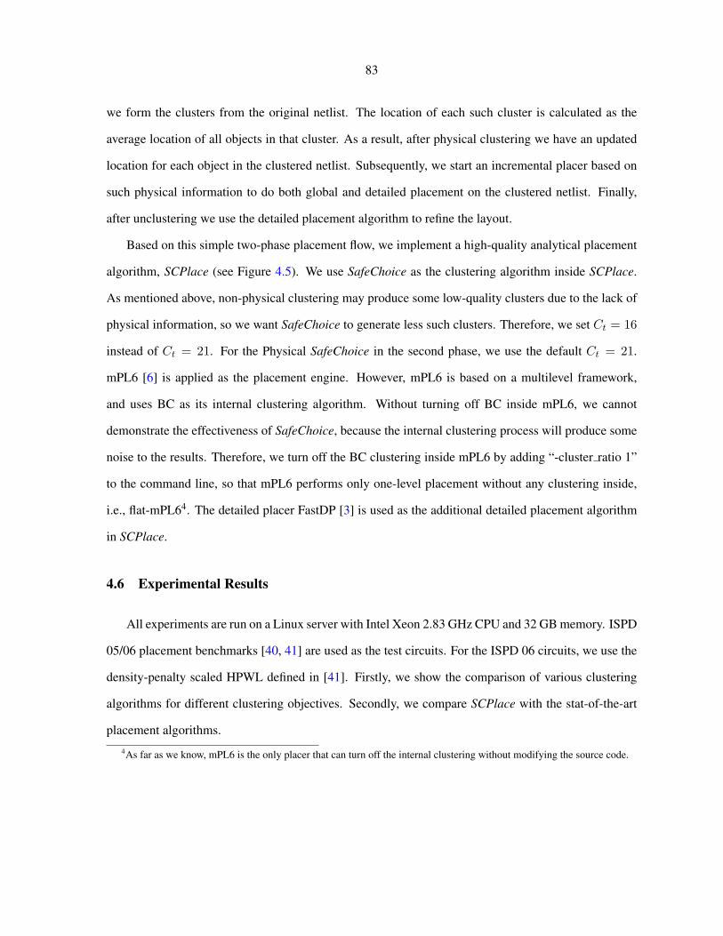
83
we form the clusters from the original netlist. The location of each such cluster is calculated as the
average location of all objects in that cluster. As a result, after physical clustering we have an updated
location for each object in the clustered netlist. Subsequently, we start an incremental placer based on
such physical information to do both global and detailed placement on the clustered netlist. Finally,
after unclustering we use the detailed placement algorithm to refine the layout.
Based on this simple two-phase placement flow, we implement a high-quality analytical placement
algorithm, SCPlace (see Figure 4.5). We use SafeChoice as the clustering algorithm inside SCPlace.
As mentioned above, non-physical clustering may produce some low-quality clusters due to the lack of
physical information, so we want SafeChoice to generate less such clusters. Therefore, we set Ct = 16
instead of Ct = 21. For the Physical SafeChoice in the second phase, we use the default Ct = 21.
mPL6 [6] is applied as the placement engine. However, mPL6 is based on a multilevel framework,
and uses BC as its internal clustering algorithm. Without turning off BC inside mPL6, we cannot
demonstrate the effectiveness of SafeChoice, because the internal clustering process will produce some
noise to the results. Therefore, we turn off the BC clustering inside mPL6 by adding “-cluster ratio 1”
to the command line, so that mPL6 performs only one-level placement without any clustering inside,
i.e., flat-mPL64. The detailed placer FastDP [3] is used as the additional detailed placement algorithm
in SCPlace.
4.6 Experimental Results
All experiments are run on a Linux server with Intel Xeon 2.83 GHz CPU and 32 GB memory. ISPD
05/06 placement benchmarks [40, 41] are used as the test circuits. For the ISPD 06 circuits, we use the
density-penalty scaled HPWL defined in [41]. Firstly, we show the comparison of various clustering
algorithms for different clustering objectives. Secondly, we compare SCPlace with the stat-of-the-art
placement algorithms.4As far as we know, mPL6 is the only placer that can turn off the internal clustering without modifying the source code.

84
Unclustering
Flat-mPL6Placement
Detailed Placement
Clustered Netlist
Clustering
Original Netlist
Figure 4.6 Experimental flow for clustering algorithm.
4.6.1 Comparison of Clustering Algorithms
We compare SC with three clustering algorithms FC [56], BC [59] and NC [60]. We implemented
FC and BC by ourselves and obtained the binary of NC from the authors [60]. For BC the lazy-
update [59] is used to speed up its runtime.
In the experiments, the clustering algorithm is applied as a pre-processing step before placement
(see Figure 4.6). We adopt mPL6 [6] as the placer. Due to the same reason mentioned in Section 4.5,
we use flat-mPL6 here. In Figure 4.6 after unclustering, we arrange the objects inside each cluster in
one row. The order among those objects are random. Subsequently the locations of all objects are
sent to flat-mPL6 for detailed placement. Because of the random order of objects within each cluster,
flat-mPL6 detailed placer alone may not be enough to generate a good result. So we apply the detailed
placer FastDP [3] to further refine the layout after flat-mPL6 detailed placement.
We normalize the results of flat-mPL6 with various pre-processing clustering to the results of flat-
mPL6 without any pre-processing clustering. For fair comparison, FastDP is applied to further refine
the output layouts from the flat-mPL6 without pre-processing clustering. We conduct five sets of exper-
iments.
I. Clustering Targeting at Safe Cluster: We compare SC-G with FC and BC. FC’s and BC’s target
γ is set the same as SC-G’s. Table 4.4 shows that SC-G’s HPWL is 2% worse than BC’s and 1% better

85
than FC’s. For both clustering time and total time, SC-G is the fastest. Note that the cost C of some
unsafe (i.e., Smax > 0) clusters may be better than some safe clusters. But unfortunately SC-G does
not form any unsafe clusters. This makes SC-G’s HPWL worse than BC’s.

86
Table 4.4 Comparison with FirstChoice and BestChoice based on SC-G’s clustering ratio (* compari-son of scaled HPWL).
Circuit Flat-mPL6 Clustering Clustering Time (s) Normalized HPWL to Flat-mPL6 Normalized Total Time to Flat-mPL6HPWL (×10e6) Time (s) Ratio (γ) FC BC SC-G FC BC SC-G FC BC SC-G
adaptec1 78.91 1197 0.80 1 2 8 1.00 1.00 1.00 1.61 1.47 1.24adaptec2 90.71 1241 0.77 2 4 10 0.99 0.99 1.00 1.73 1.63 1.43adaptec3 210.34 3923 0.71 6 23 33 1.00 0.99 0.99 1.38 1.51 1.17adaptec4 188.39 3463 0.62 9 24 38 1.00 0.99 0.98 1.76 1.70 1.28bigblue1 96.73 1424 0.77 2 4 11 0.99 0.99 1.00 1.61 1.46 1.60bigblue2 146.98 3988 0.73 142 605 101 1.00 0.99 0.99 1.57 1.54 1.52bigblue3 419.56 9486 0.58 35 123 91 0.91 0.88 0.90 1.01 1.00 1.04bigblue4 812.89 10543 0.64 273 1529 287 1.00 0.99 0.99 1.47 1.41 1.34
adaptec5* 731.47 7892 0.68 60 263 95 0.87 0.74 0.81 1.04 1.20 1.14newblue1* 109.85 17305 0.78 48 294 53 0.98 0.93 1.00 1.25 1.41 1.07newblue2* 197.44 4396 0.68 19 62 57 1.00 0.99 0.99 1.04 0.95 1.06newblue3* 320.63 10200 0.65 337 2393 228 0.94 0.96 0.95 1.29 1.65 1.67newblue4* 438.99 7779 0.71 30 137 48 0.92 0.88 0.95 0.89 0.85 0.90newblue5* 836.62 10124 0.66 363 1728 112 0.99 0.83 0.91 1.46 1.44 1.10newblue6* 520.95 7575 0.74 572 3487 204 0.99 0.98 0.98 1.78 2.14 1.42newblue7* 1076.36 19219 0.64 124 367 181 0.98 0.97 0.97 1.20 1.23 1.15
Average Normalized 1.006 5.303 1 0.974 0.944 0.963 1.381 1.413 1.258

87
II. Clustering Targeting at NetCluster’s Clustering Ratio: In this set of experiments, we compare
SC-R with FC, BC and NC based on NC’s γ. Since NC terminates when no more clusters can be formed,
it cannot reach any γ as the users desire. For each circuit the target γ of other algorithms is set the same
as NC’s. As shown in Table 4.5, SC-R consistently generates the best HPWL for all 16 test cases, except
for one case (bigblue3) where SC-R is 1% worse than BC. On average SC-R generates 4%, 1% and 5%
better HPWL than FC, BC and NC, respectively. In terms of clustering time, SC-R is 2.5× faster than
BC, while 45% and 19% slower than FC and NC, respectively. For the total time, SC-R is 1% and 7%
faster than FC and BC, while 5% slower than NC.

88
Table 4.5 Comparison with FirstChoice, BestChoice and NetCluster based on NetCluster’s clusteringratio (* comparison of scaled HPWL).
Circuit Flat-mPL6 Clustering Clustering Time (s) Normalized HPWL to Flat-mPL6 Normalized Total Time to Flat-mPL6HPWL (×10e6) Time (s) Ratio (γ) FC BC NC SC-R FC BC NC SC-R FC BC NC SC-R
adaptec1 78.91 1197 0.6381 1 3 69 20 1.00 1.00 1.01 0.99 0.92 0.91 1.15 1.04adaptec2 90.71 1241 0.5764 2 6 63 30 1.01 1.00 1.00 0.99 1.22 1.11 1.11 1.28adaptec3 210.34 3923 0.5677 7 24 62 98 1.02 0.99 0.99 0.99 1.15 1.09 1.00 1.04adaptec4 188.39 3463 0.5382 8 26 58 86 1.01 1.00 0.98 0.98 1.19 1.13 1.07 1.15bigblue1 96.73 1424 0.6128 2 5 66 23 0.99 0.98 0.98 0.98 1.19 1.08 1.21 1.13bigblue2 146.98 3988 0.5977 195 814 64 181 1.02 1.00 0.99 0.99 0.98 1.11 0.89 0.86bigblue3 419.56 9486 0.5074 36 144 53 163 0.92 0.87 0.89 0.88 0.81 0.81 0.74 0.76bigblue4 812.89 10543 0.5617 315 1696 58 588 1.01 0.99 0.99 0.99 1.21 1.27 1.10 1.19
adaptec5* 731.47 7892 0.5569 81 335 60 284 0.87 0.73 0.79 0.69 0.98 0.98 0.90 0.92newblue1* 109.85 17305 0.5674 90 472 62 125 0.93 0.90 1.03 0.86 0.82 0.88 0.77 0.83newblue2* 197.44 4396 0.5886 22 65 65 92 1.02 1.00 1.10 1.00 0.74 0.81 0.69 0.77newblue3* 320.63 10200 0.5462 427 2440 63 342 0.93 0.93 1.15 0.93 1.04 1.39 0.99 1.04newblue4* 438.99 7779 0.6357 34 159 68 109 0.92 0.86 0.93 0.85 0.63 0.62 0.59 0.58newblue5* 836.62 10124 0.5505 481 1860 58 214 0.92 0.81 0.84 0.79 1.08 1.07 0.95 1.13newblue6* 520.95 7575 0.5836 868 4871 64 755 0.99 0.97 0.97 0.97 1.14 1.78 1.01 1.05newblue7* 1076.36 19219 0.5634 142 423 60 519 0.99 0.97 0.99 0.97 0.89 0.87 0.89 0.98
Average Normalized 0.545 2.475 0.813 1 0.971 0.937 0.978 0.928 1.000 1.056 0.940 0.985

89
III. Clustering Targeting at Various Clustering Ratios: We compare SC-R with FC and BC on
five target clustering ratios γ = 0.2, 0.3, 0.4, 0.5, 0.6. In Tables 4.6 the results are organized based on
the circuits. We have two observations: (1) As γ goes lower, the clustering time increases but the total
time generally decreases; (2) To improve the HPWL, for some circuits (e.g., adaptec5) it is good to
cluster more objects. But for some circuits (e.g., newblue2) low γ degrades the HPWL. Figures 4.9, 4.8
and 4.9 shows the average normalized clustering time, HPWL and total time over all circuits for each
γ. For clustering time, SC-R is faster than BC for all γ, except for γ = 0.2 where SC-R is 12% slower.
For all γ, SC-R consistently produces the best HPWL compared with both FC and BC. Regarding the
total time SC-R is consistently faster than BC. Even though SC-R is slower than FC on clustering time,
SC-R’s total time is very comparable with FC’s, which means clusters produced by SC-R are preferred
by the placer. Furthermore, considering the significant HPWL improvements over FC and the small
percentage of clustering time over total time, we believe such slow down is acceptable.

90
Table 4.6 Comparison with FirstChoice and BestChoice on target γ = 0.2, 0.3, 0.4, 0.5, 0.6 (* com-parison of scaled HPWL).
Circuit Flat-mPL6 Clustering Clustering Time (s) Normalized HPWL to Flat-mPL6 Normalized Total Time to Flat-mPL6HPWL (×10e6) Time (s) Ratio (γ) FC BC SC-R FC BC SC-R FC BC SC-R
0.2 4 8 187 1.12 1.06 1.03 0.94 0.80 0.880.3 3 6 121 1.05 1.02 1.00 0.90 0.80 0.92
adaptec1 78.91 1197 0.4 2 5 51 1.01 1.00 0.99 0.93 0.86 1.000.5 2 4 35 1.00 1.00 0.99 0.95 0.92 0.910.6 2 3 24 1.00 0.99 0.99 1.04 1.02 1.040.2 8 16 238 1.08 1.02 1.00 1.03 0.82 1.010.3 5 12 144 1.05 0.99 0.98 1.35 1.20 1.22
adaptec2 90.71 1241 0.4 4 9 59 1.03 1.01 0.98 1.38 1.19 1.230.5 3 7 39 1.01 1.00 0.98 1.43 1.19 1.280.6 3 6 26 1.00 0.99 0.98 1.45 1.24 1.200.2 19 46 572 1.15 1.02 1.02 0.77 0.70 0.760.3 14 38 390 1.08 1.00 0.99 0.79 0.72 0.81
adaptec3 210.34 3923 0.4 11 32 162 1.04 1.00 0.99 0.94 0.74 0.730.5 9 26 114 1.04 1.00 0.98 1.28 1.16 1.170.6 7 23 80 1.01 1.00 0.98 1.35 1.21 1.230.2 16 49 403 1.08 0.99 0.99 0.81 0.70 0.790.3 13 42 276 1.04 0.98 0.98 0.82 0.74 0.77
adaptec4 188.39 3463 0.4 11 35 130 1.02 0.99 0.98 0.83 0.75 0.850.5 9 30 89 1.01 0.99 0.98 1.28 1.26 1.180.6 7 22 59 1.00 0.99 0.99 1.16 1.29 1.180.2 8 15 297 1.05 1.01 1.02 0.86 0.68 0.980.3 5 12 179 1.02 0.98 0.99 0.85 0.95 0.98
bigblue1 96.73 1424 0.4 4 9 66 1.01 0.98 0.98 0.91 0.86 0.910.5 3 7 39 1.00 0.97 0.98 1.01 0.85 0.890.6 2 6 23 1.00 0.98 0.98 1.09 1.17 1.180.2 395 1749 1162 1.15 1.07 1.05 0.84 1.05 0.920.3 344 1516 667 1.07 1.01 1.01 0.86 1.16 0.91
bigblue2 146.98 3988 0.4 302 1295 359 1.04 1.00 0.99 0.88 1.14 0.900.5 244 1005 226 1.03 0.99 0.99 0.95 1.18 0.920.6 194 796 159 1.01 1.00 0.99 1.09 1.11 0.99

91
Table 4.6 (Continued)
Comparison with FirstChoice and BestChoice on target γ = 0.2, 0.3, 0.4, 0.5, 0.6 (* comparison of scaled HPWL).Circuit Flat-mPL6 Clustering Clustering Time (s) Normalized HPWL to Flat-mPL6 Normalized Total Time to Flat-mPL6
HPWL (×10e6) Time (s) Ratio (γ) FC BC SC-R FC BC SC-R FC BC SC-R0.2 69 264 800 0.92 0.82 0.85 0.52 0.49 0.570.3 55 221 492 0.92 0.87 0.83 0.78 0.76 0.75
bigblue3 419.56 9486 0.4 46 174 241 0.92 0.84 0.85 0.90 0.81 0.820.5 36 146 158 0.93 0.88 0.88 0.93 0.95 0.910.6 30 116 89 0.91 0.88 0.89 1.00 1.01 0.910.2 633 2907 3262 1.12 1.01 1.02 1.06 1.17 1.190.3 534 2576 2220 1.06 1.00 0.99 1.19 1.44 1.24
bigblue4 812.89 10543 0.4 451 2169 1145 1.03 0.99 0.99 1.16 1.45 1.140.5 368 1819 733 1.01 0.99 0.99 1.24 1.35 1.230.6 288 1453 434 1.01 0.99 0.99 1.27 1.38 1.220.2 165 569 1424 0.77 0.63 0.62 0.52 0.56 0.660.3 139 503 984 0.83 0.66 0.63 0.52 0.52 0.62
adaptec5* 731.47 7892 0.4 114 419 456 0.84 0.68 0.65 0.61 0.58 0.590.5 93 358 324 0.86 0.72 0.69 1.07 1.29 1.070.6 73 311 204 0.88 0.73 0.70 1.23 1.32 1.150.2 169 806 781 0.91 0.88 0.81 0.13 0.24 0.230.3 149 718 527 0.91 0.86 0.80 0.23 0.49 0.41
newblue1* 109.85 17305 0.4 127 630 226 0.91 0.87 0.81 0.30 0.57 0.390.5 104 538 141 0.93 0.89 0.84 0.91 1.30 0.960.6 84 434 93 0.94 0.90 0.86 1.05 1.31 1.040.2 43 200 415 2.16 1.58 1.44 0.74 0.69 0.810.3 37 181 278 1.29 1.11 1.11 0.86 0.88 0.76
newblue2* 197.44 4396 0.4 32 164 155 1.07 1.03 1.03 0.82 0.89 0.860.5 26 128 116 1.02 1.01 1.01 1.04 0.88 0.970.6 21 65 84 1.01 1.00 1.00 0.90 0.89 0.900.2 931 3789 1010 0.98 0.89 0.89 0.50 0.76 0.500.3 783 3480 692 0.93 0.89 0.90 0.90 1.60 1.00
newblue3* 320.63 10200 0.4 630 3041 407 0.92 0.90 0.91 0.95 1.56 1.140.5 487 2546 326 0.92 0.93 0.93 1.00 1.34 1.150.6 362 2299 256 0.94 0.95 0.95 1.05 1.41 1.23

92
Table 4.6 (Continued)
Comparison with FirstChoice and BestChoice on target γ = 0.2, 0.3, 0.4, 0.5, 0.6 (* comparison of scaled HPWL).Circuit Flat-mPL6 Clustering Clustering Time (s) Normalized HPWL to Flat-mPL6 Normalized Total Time to Flat-mPL6
HPWL (×10e6) Time (s) Ratio (γ) FC BC SC-R FC BC SC-R FC BC SC-R0.2 77 334 981 0.94 0.88 0.81 0.46 0.57 0.490.3 66 302 643 0.91 0.88 0.80 0.50 0.64 0.60
newblue4* 438.99 7779 0.4 55 267 275 0.91 0.86 0.81 0.59 0.72 0.620.5 46 221 188 0.92 0.86 0.81 0.53 0.61 0.570.6 37 168 114 0.93 0.85 0.83 0.62 0.59 0.630.2 1093 3948 1483 0.94 0.70 0.78 0.64 1.02 0.620.3 877 2863 935 0.95 0.73 0.74 0.71 0.95 0.69
newblue5* 836.62 10124 0.4 693 2124 392 0.96 0.77 0.77 1.09 1.10 1.010.5 532 1903 237 0.94 0.78 0.77 1.04 1.10 0.980.6 399 1713 155 0.92 0.82 0.80 1.04 1.10 0.940.2 1941 8229 4058 1.05 0.99 0.97 1.16 1.95 1.190.3 1641 7415 2793 1.01 0.97 0.96 1.11 1.77 1.31
newblue6* 520.95 7575 0.4 1343 6558 1378 1.00 0.97 0.96 1.27 1.88 1.280.5 1082 5391 890 0.99 0.97 0.97 1.14 1.64 1.070.6 824 4535 639 0.99 0.98 0.97 1.17 1.66 1.160.2 290 948 2704 1.07 0.99 1.00 0.90 0.98 0.810.3 238 738 1774 1.02 0.97 0.97 0.78 0.80 0.93
newblue7* 1076.36 19219 0.4 197 605 891 1.00 0.97 0.97 0.79 0.74 0.950.5 159 472 596 0.99 0.97 0.97 0.76 0.72 1.000.6 126 380 422 0.98 0.97 0.97 0.93 1.00 1.03
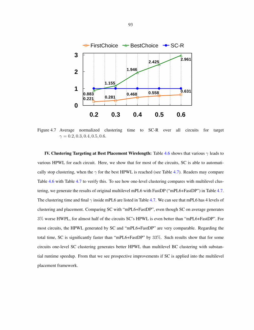
93
0.6310.5580.4680.2810.221
2.9612.425
1.946
1.155
0.883
0
1
2
3
0.2 0.3 0.4 0.5 0.6
FirstChoice BestChoice SC-R
Figure 4.7 Average normalized clustering time to SC-R over all circuits for targetγ = 0.2, 0.3, 0.4, 0.5, 0.6.
IV. Clustering Targeting at Best Placement Wirelength: Table 4.6 shows that various γ leads to
various HPWL for each circuit. Here, we show that for most of the circuits, SC is able to automati-
cally stop clustering, when the γ for the best HPWL is reached (see Table 4.7). Readers may compare
Table 4.6 with Table 4.7 to verify this. To see how one-level clustering compares with multilevel clus-
tering, we generate the results of original multilevel mPL6 with FastDP (“mPL6+FastDP”) in Table 4.7.
The clustering time and final γ inside mPL6 are listed in Table 4.7. We can see that mPL6 has 4 levels of
clustering and placement. Comparing SC with “mPL6+FastDP”, even though SC on average generates
3% worse HWPL, for almost half of the circuits SC’s HPWL is even better than “mPL6+FastDP”. For
most circuits, the HPWL generated by SC and “mPL6+FastDP” are very comparable. Regarding the
total time, SC is significantly faster than “mPL6+FastDP” by 33%. Such results show that for some
circuits one-level SC clustering generates better HPWL than multilevel BC clustering with substan-
tial runtime speedup. From that we see prospective improvements if SC is applied into the multilevel
placement framework.

94
1.093
0.9710.9760.983
1.008
0.9390.9340.9280.933
0.971
0.9230.9150.918 0.930
0.957
0.9
0.95
1
1.05
1.1
0.2 0.3 0.4 0.5 0.6
Flat-mPL6 FirstChoiceBestChoice SC-R
Figure 4.8 Average normalized HPWL to flat-mPL6 over all circuits for targetγ = 0.2, 0.3, 0.4, 0.5, 0.6.
1.091.03
0.90
0.820.74
1.171.11
0.990.96
0.82
1.07
1.020.90
0.87
0.78
0.7
0.8
0.9
1
1.1
1.2
0.2 0.3 0.4 0.5 0.6
Flat-mPL6 FirstChoiceBestChoice SC-R
Figure 4.9 Average normalized total time to flag-mPL6 over all circuits for targetγ = 0.2, 0.3, 0.4, 0.5, 0.6.

95
Table 4.7 Comparison with multilevel mPL6 (* comparison of scaled HPWL).
Circuit HPWL (×10e6) Total Time (s) SC Clustering Info. BC Clustering Info. inside mPL6Flat-mPL6 SC mPL6+FastDP Flat-mPL6 SC mPL6+FastDP Time (s) γ Time (s) Final γ # of levels
adaptec1 78.91 78.51 76.47 1197 1238 1807 76 0.33 29 0.006 4adaptec2 90.71 88.51 89.19 1241 2064 2032 73 0.36 47 0.006 4adaptec3 210.34 207.27 206.00 3923 3732 6187 228 0.33 87 0.006 4adaptec4 188.39 184.33 187.51 3463 3227 5687 208 0.31 67 0.007 4bigblue1 96.73 95.31 95.14 1424 1319 2208 109 0.32 42 0.008 4bigblue2 146.98 146.07 146.57 3988 4183 5992 458 0.36 81 0.045 4bigblue3 419.56 357.56 331.70 9486 10516 8842 420 0.30 131 0.005 4bigblue4 812.89 803.43 806.83 10543 15460 19457 1622 0.33 468 0.008 4
adaptec5* 731.47 461.99 429.97 7892 5919 10796 697 0.32 149 0.005 4newblue1* 109.85 88.10 64.72 17305 7490 2567 368 0.31 44 0.005 4newblue2* 197.44 198.35 198.90 4396 6303 7141 91 0.58 61 0.007 4newblue3* 320.63 287.76 283.25 10200 14986 9644 683 0.30 66 0.029 4newblue4* 438.99 351.02 301.89 7779 6053 9481 421 0.33 93 0.010 4newblue5* 836.62 624.26 526.98 10124 8405 16220 625 0.34 251 0.008 4newblue6* 520.95 498.44 516.43 7575 11081 13566 2059 0.33 255 0.009 4newblue7* 1076.36 1042.97 1070.08 19219 21049 32561 1159 0.34 278 0.014 4
Normalized 1 0.910 0.879 1 1.086 1.412
96
Table 4.8 Comparison with original multilevel mPL6 (* comparison of scaled HPWL).
HPWL (×10e6) Total Time (s) Clustering Info. inside SCPlaceCircuit SafeChoice Physical SafeChoice
mPL6 SCPlace mPL6 SCPlace Time (s) γ Time (s) γ # of levelsadaptec1 78.05 76.50 1769 937 54 0.43 109 0.34 1adaptec2 91.76 86.30 1940 1504 52 0.44 101 0.36 1adaptec3 214.29 204.10 5949 2981 167 0.42 192 0.34 1adaptec4 194.25 183.20 5487 2652 150 0.40 213 0.32 1bigblue1 96.75 93.58 2158 1182 60 0.43 136 0.33 1bigblue2 152.33 144.39 5842 3345 333 0.43 313 0.36 1bigblue3 343.89 336.01 8382 7682 288 0.39 302 0.31 1bigblue4 829.42 790.76 18590 12486 1219 0.42 1233 0.33 1
adaptec5* 430.42 419.72 10714 5528 459 0.41 263 0.32 1newblue1* 73.21 77.27 2489 10798 218 0.41 55 0.36 1newblue2* 201.63 194.66 7109 4642 54 0.70 79 0.61 1newblue3* 284.04 281.59 9508 13736 577 0.39 337 0.33 1newblue4* 302.04 295.98 9410 4272 288 0.43 64 0.38 1newblue5* 536.29 522.71 16085 10149 407 0.43 201 0.37 1newblue6* 521.28 494.10 13457 10877 1481 0.42 1113 0.34 1newblue7* 1083.66 1035.15 32372 23356 1003 0.43 932 0.34 1
Normalized 1.036 1 1.549 1
4.6.2 Comparison of Placement Algorithms
In this subsection, we compare SCPlace with the state-of-the-art placement algorithms.
I. Firstly, we compare SCPlace with mPL6. We run both algorithms on the same machine. The
results and the clustering information inside SCPlace are shown in Table 4.8. In terms of the HPWL,
SCPlace is consistently better than mPL6, except for one circuit (i.e., newblue1). On average, SCPlace
generates 4% better HPWL than mPL6. Regarding the total runtime, SCPlace is 55% faster than mPL6.
As mentioned in Section 4.5, in the first phase of SCPlace we set Ct = 16 rather than Ct = 21 for
non-physical SafeChoice, so that the non-physical SafeChoice will stop clustering earlier to generate
less low-quality clusters.
II. Secondly, we compare SCPlace with all other placement algorithms. Because some of the plac-
ers’ binaries are not publicly available, instead of running every placer on the same machine, we directly
cite the results from [52]. As far as we know, RQL [52] is the latest published placement algorithm in
academic area, and it generates the best results on average compared with all previous placers. The
experimental results are shown in Table 4.9. The “Previously Best” column shows the previously
best HPWL achieved by other placers for each circuit. The results are quite promising. Regarding

97
the HPWL, SCPlace is 2%, 25%, 9%, 6%, 3%, 21%, 6% and 1% better than NTUplace3, Capo10.5,
mFAR, APlace, mPL6, Dragon, Kraftwerk and RQL, respectively. Even though SCPlace is 1% worse
than the previously best approach, for 11 out of 16 circuits, SCPlace generates better results, which
means SCPlace has broken the records for 11 circuits. All of the placers here, except for Kraftwerk,
have at least four levels of placement. Using only one level of clustering and two phases of placement,
SCPlace is able to beat all of them.

98
Table 4.9 HPWL comparison with state-of-the-art placement algorithms (* comparison of scaledHPWL, † results are tuned for each circuit, the results of all other placers (except Kraftwerk2)are cited from [52] and — denotes unavailable results in [52]).
Circuit NTUplace3 [7] Capo10.5 [2] mFAR [51] APlace [4] mPL6 [6] Dragon [1] Kraftwerk2 [5] RQL [52] Previously Best SCPlace
adaptec1 80.93 91.28 — 78.35 77.91 — 82.43 77.82 77.82 76.50adaptec2 89.95 100.75 91.53† 87.31† 91.96 94.72† 92.85 88.51 87.31 86.30adaptec3 214.20 228.47 — 218.52 214.05 — 227.22 210.96 210.96 204.10adaptec4 193.74 208.35 190.84† 187.65† 194.23 200.88† 199.43 188.86 187.65 183.20bigblue1 97.28 108.60 97.70† 94.64† 96.79 102.39† 97.67 94.98 94.64 93.58bigblue2 152.20 162.92 168.70† 143.82† 152.33 159.71† 154.74 150.03 143.82 144.39bigblue3 348.48 398.49 379.95† 357.89† 344.37 380.45† 343.32 323.09 323.09 336.01bigblue4 829.16 965.30 876.28† 833.21† 829.35 903.96† 852.40 797.66 797.66 790.76
adaptec5* 448.58 494.64 476.28 520.97 431.14 500.74 449.48 443.28 431.14 419.72newblue1* 61.08 98.48 77.54 73.31 67.02 80.77 66.19 64.43 61.08 77.27newblue2* 203.39 309.53 212.90 198.24 200.93 260.83 206.53 199.60 198.24 194.66newblue3* 278.89 361.25 303.91 273.64 287.05 524.58 279.57 269.33 269.33 281.59newblue4* 301.19 362.40 324.40 384.12 299.66 341.16 309.44 308.75 299.66 295.98newblue5* 509.54 659.57 601.27 613.86 540.67 614.23 563.15 537.49 509.54 522.71newblue6* 521.65 668.66 535.96 522.73 518.70 572.53 537.59 515.69 515.69 494.10newblue7* 1099.66 1518.75 1153.76 1098.88 1082.92 1410.54 1162.12 1057.79 1057.79 1035.15
Normalized 1.02 1.25 1.09 1.06 1.03 1.21 1.06 1.01 0.99 1

99
Table 4.10 Runtime breakdown of SCPlace.
Steps in SCPlace Runtime%
Non-Physical Clustering 6%Global Placement 39%
Physical Clustering 6%Incremental Placement 45%
Detailed Placement 4%
The runtime breakdown of SCPlace is presented in Table 4.10. It shows that the total runtime
is dominated by two steps, i.e., global placement and incremental placement. Both non-physical and
physical clustering contribute only 6% of the total runtime.
4.7 Conclusion
In this chapter, we have presented SafeChoice, a novel high-quality clustering algorithm. We aim
at solving the fundamental problem — How to form safe clusters for placement. The clusters produced
by SafeChoice are definitely essential for the placer to produce a good placement. Comprehensive
experimental results show that SafeChoice is capable of producing the best clusters for the placer. Based
on SafeChoice, we derived Physical SafeChoice, and integrated it into a high-quality analytical placer,
SCPlace. Promisingly, by a simple two-phase of placement, SCPlace significantly outperforms all
state-of-the-art placement algorithms.
Our future work includes three directions: 1) To derive the safe condition for more than two vertices;
2) To develop our own placer based on SafeChoice, rather than feeding the clustered netlist to flat-mPL6
binary; 3) To integrate SafeChoice into other algorithms, e.g., hypergraph partitioning. Regarding the
last point, we can simply integrate SafeChoice into existing partitioner. Or more interestingly, we can
propose a safe condition for hypergraph partitioning, e.g., what is the safe condition to do a partition?
Finally, the source code of SafeChoice is publicly available at [39].

100
CHAPTER 5 Soft-Block Shaping in Floorplanning
Sometimes the questions are complicated and the answers are simple.
— Dr. Seuss
5.1 Introduction
Floorplanning is a very crucial step in modern VLSI designs. A good floorplan solution has a
positive impact on the placement, routing and even manufacturing. In floorplanning step, a design
contains two types of blocks, hard and soft. A hard block is a circuit block with both area and aspect
ratio 1 fixed, while a soft one has fixed area, yet flexible aspect ratio. Shaping such soft blocks plays
an important role in determining the top-level spatial structure of a chip, because the shapes of blocks
directly affect the packing quality and the area of a floorplan. However, due to the ever-increasing
complexity of ICs, the problem of shaping soft blocks is not trivial.
5.1.1 Previous Work
In slicing floorplan, researchers proposed various soft-block shaping algorithms. Stockmeyer [31]
proposed the shape curve representation used to capture different shapes of a subfloorplan. Based on
the shape curve, it is straightforward to choose the floorplan solution with the minimum cost, e.g.,
minimum floorplan area. In [32], Zimmermann extended the shape curve representation by considering
both slicing line directions when combining two blocks. Yan et al. [12] generalized the notion of slicing
tree [18] and extended the shape curve operations. Consequently, one shape curve captures significantly
more shaping and floorplan solutions.1The aspect ratio is defined as the ratio of the block height to the block width.

101
Different from slicing floorplan, the problem of shaping soft blocks to optimize the floorplan area
in non-slicing floorplan is much more complicated. Both Pan et al. [63] and Wang et al. [64] tried
to extend the slicing tree and shape curve representations to handle non-slicing floorplan. But, their
extensions are limited to some specific non-slicing structures. Instead of using the shape curve, Kang et
al. [65] adopted the bounded sliceline grid structure [66] and proposed a greedy heuristic algorithm to
select different shapes for each soft block, so that total floorplan area was minimized. Moh et al. [67]
formulated the shaping problem as a geometric programming and searched for the optimal floorplan
area using standard convex optimization. Following the same framework as in [67], Murata et al. [68]
improved the algorithm efficiency via reducing the number of variables and functions. But the algorithm
still took a long time to find a good solution. In [69], Young et al. showed that the shaping problem
for minimum floorplan area can be solved optimally by Lagrangian relaxation technique. Lin et al. [70]
changed the problem objective to minimizing the half perimeter of a floorplan, and solved it optimally
by the min-cost flow and trust region method.
For non-slicing floorplan, all previous shaping algorithms were targeting at classical floorplanning,
i.e., minimizing the floorplan area. None of them considered a predefined fixed outline in the problem
formulation. But, in the nanometer scale era classical floorplanning cannot satisfy the requirements of
hierarchical design. In contrast, fixed-outline floorplanning [17] enabling the hierarchical framework
is preferred by modern ASIC designs. Therefore, it is necessary to design a shaping algorithm in non-
slicing floorplan which can satisfy the fixed-outline constraint.
5.1.2 Our Contributions
This chapter presents an efficient, scalable and optimal slack-driven shaping (SDS) algorithm for
soft blocks in non-slicing floorplan. SDS is specifically formulated for fixed-outline floorplanning.
Given a fixed upper bound on the layout width, SDS minimizes the layout height by only shaping the
soft blocks in the design. If such upper bound is set as the width of a predefined fixed outline, SDS
is capable of optimizing the area for fixed-outline floorplanning. As far as we know, none of previous
work in non-slicing floorplan considers the fixed-outline constraint in the problem formulation. In SDS,
soft blocks are shaped iteratively. At each iteration, we shape some soft blocks to minimize the layout

102
height, with the guarantee that the layout width would not exceed the given upper bound. The amount
of change on each block is determined by globally distributing the total amount of slack to individual
block. During the whole shaping process, the layout height is monotonically reducing, and eventually
converges to an optimal solution. Essentially, we have three main contributions.
• Basic Slack-Driven Shaping: The basic slack-driven shaping algorithm is a very simple shaping
technique. Iteratively, it identifies some soft blocks, and shapes them by a slack-based shaping
scheme. The algorithm stops until there is no identified soft block. The runtime complexity in
each iteration is linear time. The basic SDS can achieve an optimal layout height for most cases.
• Optimality Conditions: To check the optimality of the shaping solution returned by the basic
SDS, two optimality conditions are proposed. We prove that if either one of the two conditions is
satisfied, the solution returned by the basic SDS is optimal.
• Slack-Driven Shaping (SDS): Based on the basic SDS and the optimality conditions, we propose
the slack-driven shaping algorithm. In SDS, a geometric programming method is applied to
improve the non-optimal solution produced by the basic SDS. SDS always returns an optimal
shaping solution.
To show the efficiency of SDS, we compare it with the two shaping algorithms in [69] and [70] on
MCNC benchmarks. Even though both of them claim their algorithms can achieve the optimal solution,
experimental results show that SDS consistently generates better solution on each circuit with signif-
icantly better runtime. On average SDS is 253× and 33× faster than [69] and [70] respectively, to
produce solutions of similar quality. We also run SDS on HB benchmarks. Experimental results show
that on average after 6%, 10%, 22% and 47% of the total iterations, the layout height is within 10%,
5%, 1% and 0.1% difference from the optimal solution, respectively.
The rest of this chapter is organized as follows. Section 5.2 describes the problem formulation.
Section 5.3 introduces the basic slack-driven shaping algorithm. Section 5.4 discusses the optimality of
a shaping solution and presents two optimality conditions. Section 5.5 describes the algorithm flow of
SDS. Experimental results are presented in Section 5.6. Finally, this chapter ends with a conclusion and
the direction of future work.

103
5.2 Problem Formulation
In the design, suppose we are given n blocks. Each block i (1 ≤ i ≤ n) has fixed area Ai.
Let wi and hi denote the width and height of block i respectively. The range of wi and hi are given
as Wmini ≤ wi ≤ Wmax
i and Hmini ≤ hi ≤ Hmax
i . If block i is a hard block, then Wmini =
Wmaxi and Hmin
i = Hmaxi . Let xi and yi denote the x and y coordinates of the bottom-left corner of
block i respectively. To model the geometric relationship among the blocks, we use the horizontal and
vertical constraint graphsGh andGv, where the vertices represent the blocks and the edges between two
vertices represent the non-overlapping constraints between the two corresponding blocks. In Gh, we
add two dummy vertices 0 and n+ 1 that represent the left-most and right-most boundary of the layout
respectively. Similarly, in Gv we add two dummy vertices 0 and n + 1 that represent the bottom-most
and top-most boundary of the layout respectively. The area of the dummy vertices is 0. We have x0 = 0
and y0 = 0. Vertices 0 and n+ 1 are defined as the source and the sink in the graphs respectively. Thus,
in both Gh and Gv, we add one edge from the source to each vertex that does not have any incoming
edge, and add one edge from each vertex that does not have any outgoing edge to the sink.
In our problem formulation, we assume the constraint graphs Gh and Gv are given. Given an upper
bound on the layout width as W , we want to minimize the layout height yn+1 by only shaping the
soft blocks in the design, such that the layout width xn+1 ≤ W . Such problem can be mathematically
formulated as follows:

104
Problem 1. Height Minimization with Fixed Upper-Bound Width
Minimize yn+1
subject to xn+1 ≤W
xj ≥ xi + wi, ∀(i, j) ∈ Gh
yj ≥ yi + hi, ∀(i, j) ∈ Gv
Wmini ≤ wi ≤Wmax
i , 1 ≤ i ≤ n
Hmini ≤ hi ≤ Hmax
i , 1 ≤ i ≤ n
wihi = Ai, 1 ≤ i ≤ n
x0 = 0
y0 = 0
It is clear that if W is set as the width of a predefined fixed outline, Problem 1 can be applied in
fixed-outline floorplanning.
5.3 Basic Slack-Driven Shaping
In this section, we present the basic slack-driven shaping algorithm, which solves Problem 1 opti-
mally for most cases.
First of all, we introduce some notations used in the discussion. Given the constraint graphs and the
shape of the blocks, we can pack the blocks to four lines, i.e., the left (LL), right (RL), bottom (BL)
and top (TL) lines. LL, RL, BL and TL are set as “x = 0”, “x = W ”, “y = 0” and “y = yn+1”,
respectively. Let ∆xi denote the difference of xi when packing block i to RL and LL. Similarly,
∆yi denotes the difference of yi when packing block i to TL and BL. For block i (1 ≤ i ≤ n), the
horizontal slack shi and vertical slack svi are calculated as follows:
shi = max(0,∆xi)
svi = max(0,∆yi)
In Gh, given any path 2 from the source to the sink, if for all blocks on this path, their horizontal slacks
are equal to zero, then we define such path as a horizontal critical path (HCP). The length of one HCP2By default, all paths mentioned in this chapter are from the source to the sink in the constraint graph.
105
is the summation of the width of blocks on this path. Similarly, we can define the vertical critical path
(VCP) and the length of one VCP is the summation of the height of blocks on this path. Note that,
because we set RL as the “x = W ” line, if xn+1 < W , then there is no HCP in Gh.
The algorithm flow of the basic SDS is simple and straightforward. The soft blocks are shaped
iteratively. At each iteration, we apply the following operations:
1. Shape the soft blocks on all VCPs by increasing the width and decreasing the height. This reduces
the lengths of the VCPs.
2. Shape the soft blocks on all HCPs by decreasing the width and increasing the height. This reduces
the lengths of the HCPs.
The purpose of the first operation is to minimize the layout height yn+1 by decreasing the lengths of
all VCPs. As mentioned previously, if xn+1 < W then there is no HCP. Thus, the second operation
is applied only if xn+1 = W . This operation seems to be unnecessary, yet actually is critical for the
proof of the optimality conditions. The purpose of this operation will be explained in Section 5.4. At
each iteration, we first globally distribute the total amount of slack reduction to the soft blocks, and then
locally shape each individual soft block on the cirtical paths based on the allocated amount of slack
reduction. The algorithm stops until we cannot find any soft block to shape on the critical paths. During
the whole shaping process, the layout height yn+1 is monotonically decreasing and thus the algorithm
always converges.
In the following subsections, we first identify which soft blocks to be shaped (which we called target
soft blocks) at each iteration. Secondly, we mathematically derive the shaping scheme on the target soft
blocks. Finally, we present the algorithm flow of the basic slack-driven shaping.

106
5.3.1 Target Soft Blocks
For a given shaping solution, the set of n blocks can be divided into the following seven disjoint
subsets (I–VII).
Subset I = {block i is hard}
Subset II = {block i is soft} ∩ {shi 6= 0, svi 6= 0}
Subset III = {block i is soft} ∩ {shi = 0, svi = 0}
Subset IV = {block i is soft} ∩ {shi 6= 0, svi = 0} ∩ {wi 6= Wmaxi }
Subset V = {block i is soft} ∩ {shi 6= 0, svi = 0} ∩ {wi = Wmaxi }
Subset VI = {block i is soft} ∩ {shi = 0, svi 6= 0} ∩ {hi 6= Hmaxi }
Subset VII = {block i is soft} ∩ {shi = 0, svi 6= 0} ∩ {hi = Hmaxi }
Based on the definitions of critical paths, we have the following observations.
Observation 1. If block i ∈ subset II, then i is not on any HCP nor VCP.
Observation 2. If block i ∈ subset III, then i is on both HCP and VCP, i.e., at the intersection of some
HCP and some VCP.
Observation 3. If block i ∈ subset IV or V, then i is on some VCP but not on any HCP.
Observation 4. If block i ∈ subset VI or VII, then i is on some HCP but not on any VCP.
As mentioned previously, yn+1 can be minimized by reducing the height of the soft blocks on the
vertical cricital paths, and such block-height reduction will result in a decrease on the horizontal slacks
of those soft blocks. From the above observations, only soft blocks in subsets III, IV and V are on the
vertical critical paths. However, for block i ∈ subset III, shi = 0, which means its horizontal slack
cannot be further reduced. And for block i ∈ subset V, wi = Wmaxi , which means its height cannot
be further reduced. As a result, to minimize yn+1 we can only shape blocks in subset IV. Similarly, we
conclude that whenever we need to reduce xn+1 we can only shape blocks in subset VI. For the hard
blocks in subset I, they cannot be shaped anyway.
Therefore, the target soft blocks are blocks in subsets IV and VI.
107
5.3.2 Shaping Scheme
Let δhi denote the amount of increase on wi for block i ∈ subset IV, and δvi denote the amount of
increase on hi for block i ∈ subset VI. In the remaining part of this subsection, we present the shaping
scheme to shape the target soft block i ∈ subset IV by setting δhi . Similar shaping scheme is applied to
shape the target soft block i ∈ subset VI by setting δvi . By default, all blocks mentioned in the following
part are referring to the target soft blocks in subset IV.
We use “i ∈ p” to denote that block i is on a path p in Gh. Suppose the maximum horizontal slack
over all blocks on p is spmax. Basically, spmax gives us a budget on the total amount of increase on the
block width along this path. If∑
i∈p δhi > spmax, then after shaping, we have xn+1 > W , which violates
the “xn+1 ≤ W ” constraint. Therefore, we have to set δhi accordingly, such that∑
i∈p δhi ≤ spmax for
all p in Gh.
To determine the value of δhi , we first define a distribution ratio αpi (αpi ≥ 0) for block i ∈ p. We
assign the value of αpi , such that ∑i∈p
αpi = 1
Lemma 6. For any path p in Gh, we have
∑i∈p
αpi shi ≤ spmax
Proof. Because spmax = MAXi∈p(shi ), this lemma can be proved as follows:
∑i∈p
αpi shi ≤
∑i∈p
αpi spmax = spmax
∑i∈p
αpi = spmax
Based on Lemma 6, for a single path p, it is obvious that if δhi ≤ αpi shi (i ∈ p), then we can guarantee∑
i∈p δhi ≤ s
pmax.
More generally, if there are multiple paths going through block i (1 ≤ i ≤ n), then δhi needs to
satisfy the following inequality:
δhi ≤ αpi shi ,∀p ∈ P hi (5.1)

108
where P hi is the set of paths in Gh going through block i. Inequality 5.1 is equivalent to the following
inequality.
δhi ≤ MINp∈Ph
i
(αpi )shi (5.2)
Essentially, Inequality 5.2 gives an upper bound on the amount of increase onwi for block i ∈ subset IV.
For block i ∈ p, the distribution ratio is set as follows:
αpi =
0 i is the source or the sink
Wmaxi −wiP
k∈p(Wmaxk −wk) otherwise
(5.3)
The insight is that if we allocate more slack reduction to the blocks that have potentially more room to
be shaped, the algorithm will converge faster. And we allocate zero amount of slack reduction to the
dummy blocks at the source and the sink in Gh. Based on Equation 5.3, Inequality 5.2 can be rewritten
as follows (1 ≤ i ≤ n):
δhi ≤(Wmax
i − wi)shiMAXp∈Ph
i
(∑
k∈p(Wmaxk − wk))
(5.4)
From the above inequality, to calculate the upper bound of δhi , we need to obtain the value of three
terms, (Wmaxi −wi), shi and MAXp∈Ph
i(∑
k∈p(Wmaxk −wk)). The first term can be obtained in constant
time. Using the longest path algorithm, shi for all i can be calculated in linear time. A trivial approach
to calculate the third term is via traversing each path in Gh. This takes exponential time, which is not
practical. Thus, we propose a dynamic programming (DP) based approach, which takes linear time to
get MAXp∈Phi
(∑
k∈p(Wmaxk − wk)).
In Gh, suppose vertex i (0 ≤ i ≤ n + 1) has in-coming edges coming from the vertices in the set
V ini , and out-going edges going to the vertices in the set V out
i . Let P ini denote the set of paths that
start at the source and end at vertex i in Gh, and P outi denote the set of paths that start at vertex i and
end at the sink in Gh. For the source of Gh, we have V in0 = φ and P in0 = φ. For the sink of Gh,
we have V outn+1 = φ and P outn+1 = φ. We notice that MAXp∈Ph
i(∑
k∈p(Wmaxk − wk)) can be calculated

109
recursively by the following equations.
MAXp∈P in
0
(∑k∈p
(Wmaxk − wk)) = 0
MAXp∈P out
n+1
(∑k∈p
(Wmaxk − wk)) = 0
MAXp∈P in
i
(∑k∈p
(Wmaxk − wk)) = MAX
j∈V ini
(MAXp∈P in
j
(∑k∈p
(Wmaxk − wk)))
+(Wmaxi − wi) (5.5)
MAXp∈P out
i
(∑k∈p
(Wmaxk − wk)) = MAX
j∈V outi
(MAXp∈P out
j
(∑k∈p
(Wmaxk − wk))
+(Wmaxi − wi) (5.6)
MAXp∈Ph
i
(∑k∈p
(Wmaxk − wk)) = MAX
p∈P ini
(∑k∈p
(Wmaxk − wk))
+MAXp∈P out
i
(∑k∈p
(Wmaxk − wk))
−(Wmaxi − wi) (5.7)
Based on the equations above, the DP-based approach can be applied as follows (1 ≤ i ≤ n):
1. Firstly, we apply topological sort algorithm on Gh.
2. Secondly, we scan the sorted vertices from the source to the sink, and calculate MAXp∈P ini
(∑
k∈p(Wmaxk −
wk)) by Equation 5.5.
3. Thirdly, we scan the sorted vertices from the sink to the source, and calculate MAXp∈P outi
(∑
k∈p(Wmaxk −
wk)) by Equation 5.6.
4. Finally, MINp∈Phi
(∑
k∈p(Wmaxk − wk)) is obtained by Equation 5.7.
It is clear that by the DP-based approach, the whole process of calculating the upper bound of δhi for all
i takes linear time.
5.3.3 Flow of Basic Slack-Driven Shaping
The algorithm flow of basic slack-driven shaping is shown in Figure 5.1.
In the algorithm flow shown in Figure 5.1, for each block i in the design, we set its initial width
wi = Wmini (1 ≤ i ≤ n). Based on the input Gh, Gv and initial block shape, we can calculate an initial

110
Basic Slack-Driven ShapingInput: wi = Wmin
i (∀1 ≤ i ≤ n);Gh and Gv;upper-bound width W .
Output: optimized yn+1, wi and hi.Begin1. Set LL, BL and RL to “x = 0”, “y = 0” and “x = W ”.2. Pack blocks to LL and use longest path algorithm to get xn+1.3. If xn+1 > W ,4. Return no feasible solution.5. Else,6. Repeat7. Pack blocks to BL and use longest path algorithm to get yn+1.8. Set TL to “y = yn+1”.9. Pack blocks to LL, RL and TL, respectively.10. Calculate shi and svi .11. Find target soft blocks.12. If there are target soft blocks,13. ∀j ∈ subset IV, increase wj by δhj = MINp∈Ph
j(αpj )s
hj ;
14. ∀j ∈ subset VI, increase hj by δvj = β ×MINp∈P vj(αpj )s
vj .
15. Until there is no target soft block.End
Figure 5.1 Flow of basic slack-driven shaping.
111
value of xn+1. If this initial value is already bigger than W , then Problem 1 is not feasible. At each
iteration we set δvj = β ×MINp∈P vj
(αpj )svj for target soft block j ∈ subset VI. By default, β = 100%,
which means we use up all available vertical slacks every time. One potential problem with this strategy
is that the layout height yn+1 may remain the same, i.e., never decreasing. This is because after one
iteration of shaping, the length of some non-critical vertical path increases, and consequently its length
may become equivalent to the length of the VCP in the previous iteration. To solve this issue, in the
implementation whenever we detect that yn+1 does not change for more than two iterations, we will set
β = 90%. That is we only allocate part of the available slacks to the soft blocks. For δhj , we always set
it at its upper bound.
Because in each iteration the total increase on width or height of the target soft blocks would not
exceed the budget, we can guarantee that the layout would not be outside of the four lines after shaping.
As iteratively we set TL to the updated “y = yn+1” line, yn+1 will be monotonically decreasing during
the whole shaping process. Different from TL, because we set RL to the fixed “x = W ” line, during
the shaping process xn+1 may be bouncing i.e., sometimes increasing and sometimes decreasing, yet
always no more than W . The shaping process stops when there is no target soft block.
5.4 Optimality Conditions
For most cases, in the basic SDS the layout height yn+1 will converge to an optimal solution of
Problem 1. However, sometimes the solution may be non-optimal as the one shown in Figure 5.2-(a).
The layout in Figure 5.2-(a) contains four soft blocks 1, 2, 3 and 4, where Ai = 4, Wmini = 1 and
Wmaxi = 4 (1 ≤ i ≤ 4). The given upper-bound width W = 5. In the layout, w1 = w3 = 4 and
w2 = w4 = 1. There is no target soft block on any one of the four critical paths (i.e., two HCPs and
two VCPs), so the basic SDS returns yn+1 = 5. But the optimal layout height should be 3.2, when
w1 = w2 = w3 = w4 = 2.5 as shown in Figure 5.2-(b). In this section, we will look into this issue
and present the optimality conditions for the shaping solution returned by the basic SDS.
Let L represent a shaping solution generated by the basic SDS in Figure 5.1. All proof in this
section are established based on the fact that the only remaining soft blocks that could be shaped to
possibly improve L are the ones in subset III. This is because L is the solution returned by the basic
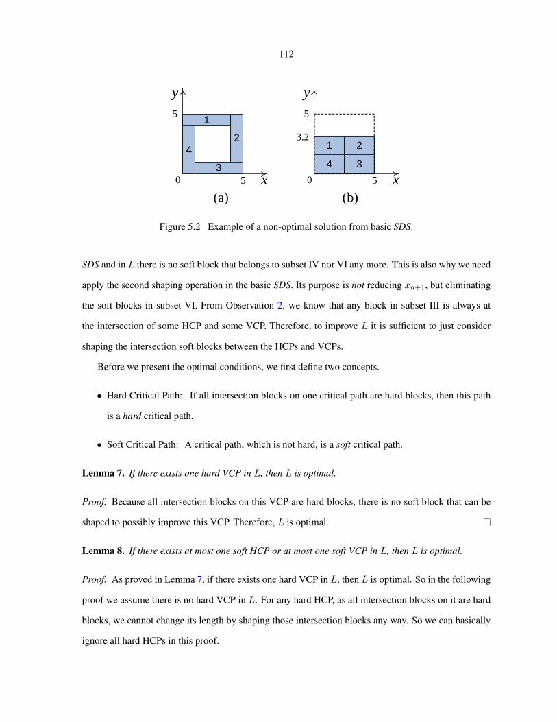
112
42
x5
y5
0
(a)
4
x5
y5
0
(b)
1
3
23.2
3
1
Figure 5.2 Example of a non-optimal solution from basic SDS.
SDS and in L there is no soft block that belongs to subset IV nor VI any more. This is also why we need
apply the second shaping operation in the basic SDS. Its purpose is not reducing xn+1, but eliminating
the soft blocks in subset VI. From Observation 2, we know that any block in subset III is always at
the intersection of some HCP and some VCP. Therefore, to improve L it is sufficient to just consider
shaping the intersection soft blocks between the HCPs and VCPs.
Before we present the optimal conditions, we first define two concepts.
• Hard Critical Path: If all intersection blocks on one critical path are hard blocks, then this path
is a hard critical path.
• Soft Critical Path: A critical path, which is not hard, is a soft critical path.
Lemma 7. If there exists one hard VCP in L, then L is optimal.
Proof. Because all intersection blocks on this VCP are hard blocks, there is no soft block that can be
shaped to possibly improve this VCP. Therefore, L is optimal.
Lemma 8. If there exists at most one soft HCP or at most one soft VCP in L, then L is optimal.
Proof. As proved in Lemma 7, if there exists one hard VCP in L, then L is optimal. So in the following
proof we assume there is no hard VCP in L. For any hard HCP, as all intersection blocks on it are hard
blocks, we cannot change its length by shaping those intersection blocks any way. So we can basically
ignore all hard HCPs in this proof.
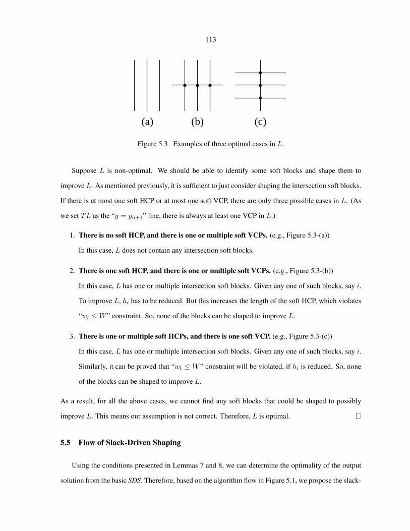
113
(a) (b) (c)
Figure 5.3 Examples of three optimal cases in L.
Suppose L is non-optimal. We should be able to identify some soft blocks and shape them to
improve L. As mentioned previously, it is sufficient to just consider shaping the intersection soft blocks.
If there is at most one soft HCP or at most one soft VCP, there are only three possible cases in L. (As
we set TL as the “y = yn+1” line, there is always at least one VCP in L.)
1. There is no soft HCP, and there is one or multiple soft VCPs. (e.g., Figure 5.3-(a))
In this case, L does not contain any intersection soft blocks.
2. There is one soft HCP, and there is one or multiple soft VCPs. (e.g., Figure 5.3-(b))
In this case, L has one or multiple intersection soft blocks. Given any one of such blocks, say i.
To improve L, hi has to be reduced. But this increases the length of the soft HCP, which violates
“wl ≤W ” constraint. So, none of the blocks can be shaped to improve L.
3. There is one or multiple soft HCPs, and there is one soft VCP. (e.g., Figure 5.3-(c))
In this case, L has one or multiple intersection soft blocks. Given any one of such blocks, say i.
Similarly, it can be proved that “wl ≤ W ” constraint will be violated, if hi is reduced. So, none
of the blocks can be shaped to improve L.
As a result, for all the above cases, we cannot find any soft blocks that could be shaped to possibly
improve L. This means our assumption is not correct. Therefore, L is optimal.
5.5 Flow of Slack-Driven Shaping
Using the conditions presented in Lemmas 7 and 8, we can determine the optimality of the output
solution from the basic SDS. Therefore, based on the algorithm flow in Figure 5.1, we propose the slack-

114
driven shaping algorithm shown in Figure 5.4. SDS always returns an optimal solution for Problem 1.
Slack-Driven ShapingInput: wi = Wmin
i (∀1 ≤ i ≤ n);Gh and Gv;upper-bound width W .
Output: optimal yn+1, wi and hi.Begin1. Set LL, BL and RL to “x = 0”, “y = 0” and “x = W ”.2. Pack blocks to LL and use longest path algorithm to get xn+1.3. If xn+1 > W ,4. Return no feasible solution.5. Else,6. Repeat7. Pack blocks to BL and use longest path algorithm to get yn+1.8. Set TL to “y = yn+1”.9. Pack blocks to LL, RL and TL, respectively.10. Calculate shi and svi .11. Find target soft blocks.12. If there are target soft blocks,13. ∀j ∈ subset IV, increase wj by δhj = MINp∈Ph
j(αpj )s
hj ;
14. ∀j ∈ subset VI, increase hj by δvj = β ×MINp∈P vj(αpj )s
vj .
15. Else,16. If Lemma 7 or 8 is satisfied,17. L is optimal.18. Else,19. Improve L by a single step of geometric programming.20. If no optimal solution is obtained,21. Go to Line 7.22. Else,23. L is optimal.24. Until L is optimal.End
Figure 5.4 Flow of slack-driven shaping.
The differences between SDS and the basic version are starting from line 15 in Figure 5.4. When
there is not target soft block, instead of terminating the algorithm, SDS will first check the optimality of
L, and if it is not optimal, L will be improved via geometric programming. The algorithm stops when
an optimal solution is obtained.
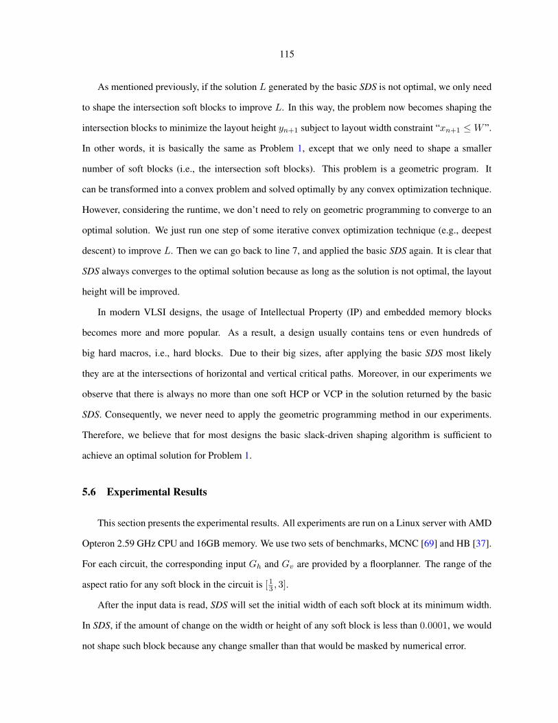
115
As mentioned previously, if the solution L generated by the basic SDS is not optimal, we only need
to shape the intersection soft blocks to improve L. In this way, the problem now becomes shaping the
intersection blocks to minimize the layout height yn+1 subject to layout width constraint “xn+1 ≤W ”.
In other words, it is basically the same as Problem 1, except that we only need to shape a smaller
number of soft blocks (i.e., the intersection soft blocks). This problem is a geometric program. It
can be transformed into a convex problem and solved optimally by any convex optimization technique.
However, considering the runtime, we don’t need to rely on geometric programming to converge to an
optimal solution. We just run one step of some iterative convex optimization technique (e.g., deepest
descent) to improve L. Then we can go back to line 7, and applied the basic SDS again. It is clear that
SDS always converges to the optimal solution because as long as the solution is not optimal, the layout
height will be improved.
In modern VLSI designs, the usage of Intellectual Property (IP) and embedded memory blocks
becomes more and more popular. As a result, a design usually contains tens or even hundreds of
big hard macros, i.e., hard blocks. Due to their big sizes, after applying the basic SDS most likely
they are at the intersections of horizontal and vertical critical paths. Moreover, in our experiments we
observe that there is always no more than one soft HCP or VCP in the solution returned by the basic
SDS. Consequently, we never need to apply the geometric programming method in our experiments.
Therefore, we believe that for most designs the basic slack-driven shaping algorithm is sufficient to
achieve an optimal solution for Problem 1.
5.6 Experimental Results
This section presents the experimental results. All experiments are run on a Linux server with AMD
Opteron 2.59 GHz CPU and 16GB memory. We use two sets of benchmarks, MCNC [69] and HB [37].
For each circuit, the corresponding input Gh and Gv are provided by a floorplanner. The range of the
aspect ratio for any soft block in the circuit is [13 , 3].
After the input data is read, SDS will set the initial width of each soft block at its minimum width.
In SDS, if the amount of change on the width or height of any soft block is less than 0.0001, we would
not shape such block because any change smaller than that would be masked by numerical error.

116
5.6.1 Experiments on MCNC Benchmarks
Using the MCNC benchmarks we compare SDS with the two shaping algorithms in [69] and [70].
All blocks in these circuits are soft blocks. The source codes of [69] and [70] are obtained from the
authors.
In fact, these three shaping algorithms cannot be directly compared, because their optimization
objectives are all different:
• [69] is minimizing the layout area xn+1yn+1;
• [70] is minimizing the layout half perimeter xn+1 + yn+1;
• SDS is minimizing the layout height yn+1, s.t. xn+1 ≤W .
Still, to make some meaningful comparisons as best as we can, we setup the experiment in the following
way.
• We do two groups of experiment: 1) SDS v.s. [69]; 2) SDS v.s. [70].
• As the circuit size are all very small, to do some meaningful comparison on the runtime, in each
group we run both shaping algorithms 1000 times with the same input data.
• For group 1, we run [69] first, and use the returned final width from [69] as the input upper-bound
width W for SDS. Similar procedure is applied for group 2.
• For groups 1 and 2, we compare the final results based on [69]’s and [70]’s objective respectively.
Table 5.1 shows the results on group 1. The column “ws(%)” gives the white space percentage
over the total block area in the final layout. For all five circuits SDS achieves significantly better results
on the floorplan area. On average, SDS achieves 394× smaller white space and 23× faster runtime
than [69]. In the last column, we report the runtime SDS takes to converge to a solution that is better
than [69]. To just get a slightly better solution than [69], on average SDS uses 253× faster runtime.
As pointed out by [70], [69] does not transform the problem into a convex problem before applying
Lagrangian relaxation. Hence, the algorithm [69] may not converge to an optimal solution.
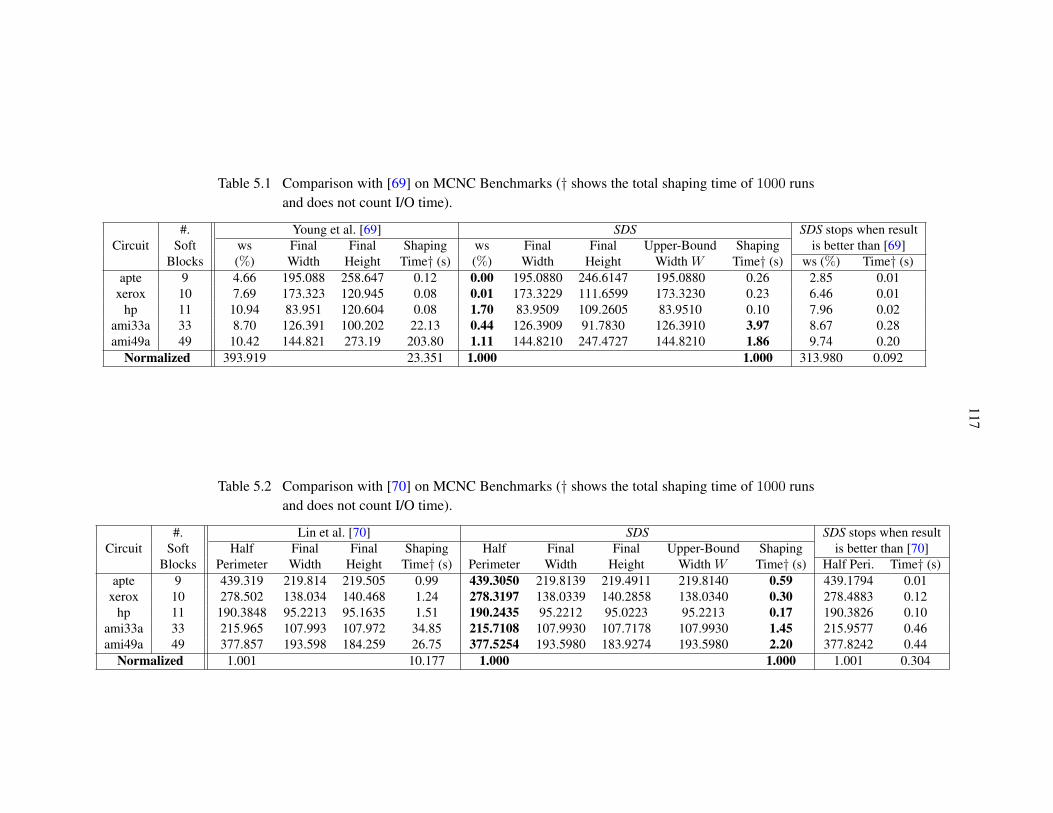
117
Table 5.1 Comparison with [69] on MCNC Benchmarks († shows the total shaping time of 1000 runsand does not count I/O time).
#. Young et al. [69] SDS SDS stops when resultCircuit Soft ws Final Final Shaping ws Final Final Upper-Bound Shaping is better than [69]
Blocks (%) Width Height Time† (s) (%) Width Height Width W Time† (s) ws (%) Time† (s)apte 9 4.66 195.088 258.647 0.12 0.00 195.0880 246.6147 195.0880 0.26 2.85 0.01
xerox 10 7.69 173.323 120.945 0.08 0.01 173.3229 111.6599 173.3230 0.23 6.46 0.01hp 11 10.94 83.951 120.604 0.08 1.70 83.9509 109.2605 83.9510 0.10 7.96 0.02
ami33a 33 8.70 126.391 100.202 22.13 0.44 126.3909 91.7830 126.3910 3.97 8.67 0.28ami49a 49 10.42 144.821 273.19 203.80 1.11 144.8210 247.4727 144.8210 1.86 9.74 0.20
Normalized 393.919 23.351 1.000 1.000 313.980 0.092
Table 5.2 Comparison with [70] on MCNC Benchmarks († shows the total shaping time of 1000 runsand does not count I/O time).
#. Lin et al. [70] SDS SDS stops when resultCircuit Soft Half Final Final Shaping Half Final Final Upper-Bound Shaping is better than [70]
Blocks Perimeter Width Height Time† (s) Perimeter Width Height Width W Time† (s) Half Peri. Time† (s)apte 9 439.319 219.814 219.505 0.99 439.3050 219.8139 219.4911 219.8140 0.59 439.1794 0.01
xerox 10 278.502 138.034 140.468 1.24 278.3197 138.0339 140.2858 138.0340 0.30 278.4883 0.12hp 11 190.3848 95.2213 95.1635 1.51 190.2435 95.2212 95.0223 95.2213 0.17 190.3826 0.10
ami33a 33 215.965 107.993 107.972 34.85 215.7108 107.9930 107.7178 107.9930 1.45 215.9577 0.46ami49a 49 377.857 193.598 184.259 26.75 377.5254 193.5980 183.9274 193.5980 2.20 377.8242 0.44
Normalized 1.001 10.177 1.000 1.000 1.001 0.304
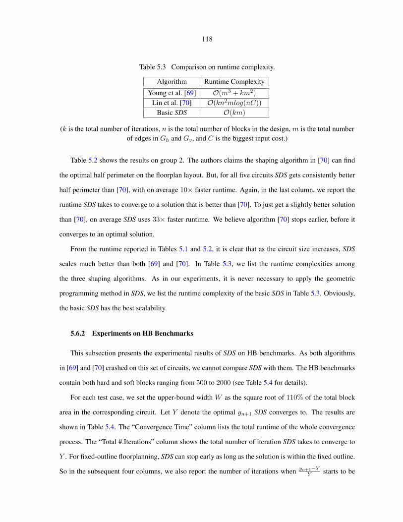
118
Table 5.3 Comparison on runtime complexity.
Algorithm Runtime Complexity
Young et al. [69] O(m3 + km2)Lin et al. [70] O(kn2mlog(nC))
Basic SDS O(km)
(k is the total number of iterations, n is the total number of blocks in the design, m is the total numberof edges in Gh and Gv, and C is the biggest input cost.)
Table 5.2 shows the results on group 2. The authors claims the shaping algorithm in [70] can find
the optimal half perimeter on the floorplan layout. But, for all five circuits SDS gets consistently better
half perimeter than [70], with on average 10× faster runtime. Again, in the last column, we report the
runtime SDS takes to converge to a solution that is better than [70]. To just get a slightly better solution
than [70], on average SDS uses 33× faster runtime. We believe algorithm [70] stops earlier, before it
converges to an optimal solution.
From the runtime reported in Tables 5.1 and 5.2, it is clear that as the circuit size increases, SDS
scales much better than both [69] and [70]. In Table 5.3, we list the runtime complexities among
the three shaping algorithms. As in our experiments, it is never necessary to apply the geometric
programming method in SDS, we list the runtime complexity of the basic SDS in Table 5.3. Obviously,
the basic SDS has the best scalability.
5.6.2 Experiments on HB Benchmarks
This subsection presents the experimental results of SDS on HB benchmarks. As both algorithms
in [69] and [70] crashed on this set of circuits, we cannot compare SDS with them. The HB benchmarks
contain both hard and soft blocks ranging from 500 to 2000 (see Table 5.4 for details).
For each test case, we set the upper-bound width W as the square root of 110% of the total block
area in the corresponding circuit. Let Y denote the optimal yn+1 SDS converges to. The results are
shown in Table 5.4. The “Convergence Time” column lists the total runtime of the whole convergence
process. The “Total #.Iterations” column shows the total number of iteration SDS takes to converge to
Y . For fixed-outline floorplanning, SDS can stop early as long as the solution is within the fixed outline.
So in the subsequent four columns, we also report the number of iterations when yn+1−YY starts to be

119
less than 10%, 5%, 1% and 0.1%, respectively. The average total convergence time is 1.18 second. SDS
takes average 1901 iterations to converge to Y . The four percentage numbers in the last row shows
that on average after 6%, 10%, 22% and 47% of the total number of iterations, SDS converges to the
layout height that is within 10%, 5%, 1% and 0.1% difference from Y , respectively. In order to show
the convergence process more intuitively, we plot out the convergence graphs of yn+1 for four circuits
in Figure 5.5(a)-5.5(d). In the curves, the four blue arrows point to the four points when yn+1 becomes
less than 10%, 5%, 1% and 0.1% difference from Y , respectively.
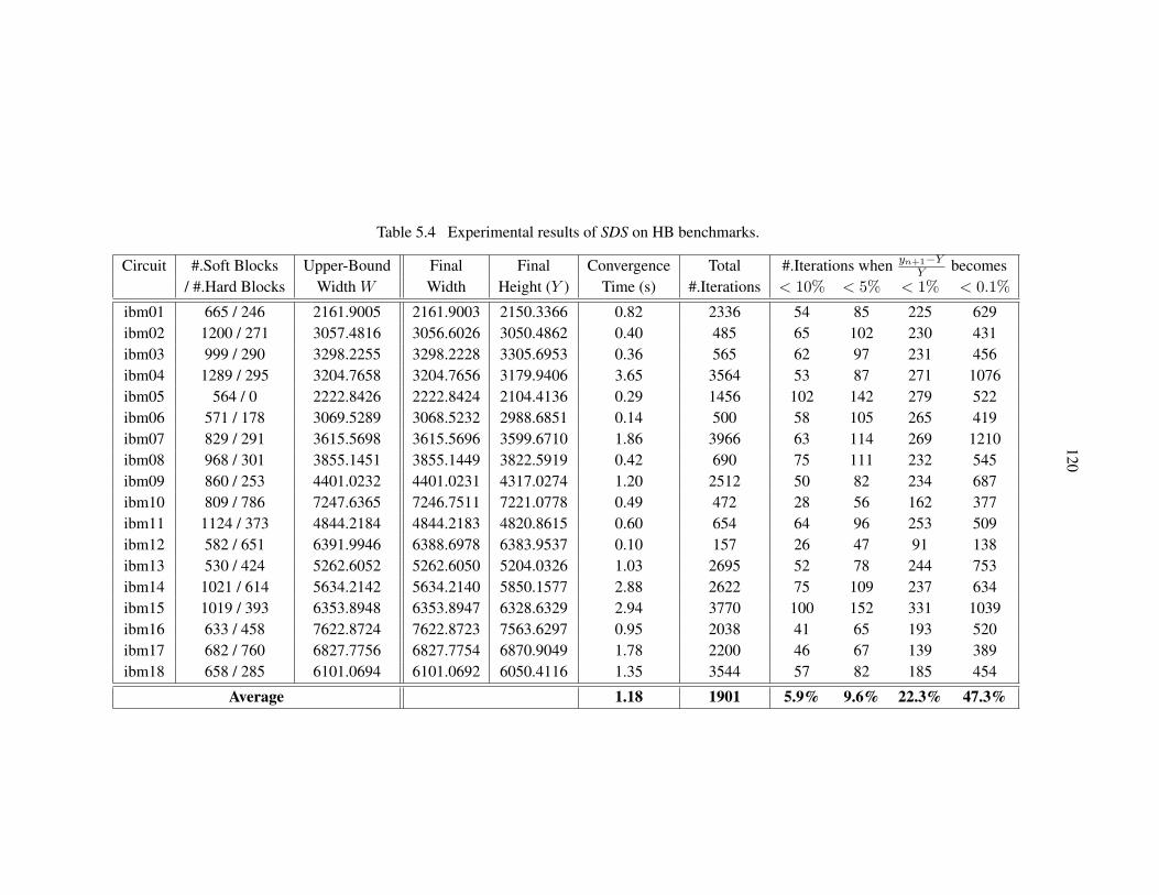
120
Table 5.4 Experimental results of SDS on HB benchmarks.
Circuit #.Soft Blocks Upper-Bound Final Final Convergence Total #.Iterations when yn+1−YY becomes
/ #.Hard Blocks Width W Width Height (Y ) Time (s) #.Iterations < 10% < 5% < 1% < 0.1%
ibm01 665 / 246 2161.9005 2161.9003 2150.3366 0.82 2336 54 85 225 629ibm02 1200 / 271 3057.4816 3056.6026 3050.4862 0.40 485 65 102 230 431ibm03 999 / 290 3298.2255 3298.2228 3305.6953 0.36 565 62 97 231 456ibm04 1289 / 295 3204.7658 3204.7656 3179.9406 3.65 3564 53 87 271 1076ibm05 564 / 0 2222.8426 2222.8424 2104.4136 0.29 1456 102 142 279 522ibm06 571 / 178 3069.5289 3068.5232 2988.6851 0.14 500 58 105 265 419ibm07 829 / 291 3615.5698 3615.5696 3599.6710 1.86 3966 63 114 269 1210ibm08 968 / 301 3855.1451 3855.1449 3822.5919 0.42 690 75 111 232 545ibm09 860 / 253 4401.0232 4401.0231 4317.0274 1.20 2512 50 82 234 687ibm10 809 / 786 7247.6365 7246.7511 7221.0778 0.49 472 28 56 162 377ibm11 1124 / 373 4844.2184 4844.2183 4820.8615 0.60 654 64 96 253 509ibm12 582 / 651 6391.9946 6388.6978 6383.9537 0.10 157 26 47 91 138ibm13 530 / 424 5262.6052 5262.6050 5204.0326 1.03 2695 52 78 244 753ibm14 1021 / 614 5634.2142 5634.2140 5850.1577 2.88 2622 75 109 237 634ibm15 1019 / 393 6353.8948 6353.8947 6328.6329 2.94 3770 100 152 331 1039ibm16 633 / 458 7622.8724 7622.8723 7563.6297 0.95 2038 41 65 193 520ibm17 682 / 760 6827.7756 6827.7754 6870.9049 1.78 2200 46 67 139 389ibm18 658 / 285 6101.0694 6101.0692 6050.4116 1.35 3544 57 82 185 454
Average 1.18 1901 5.9% 9.6% 22.3% 47.3%
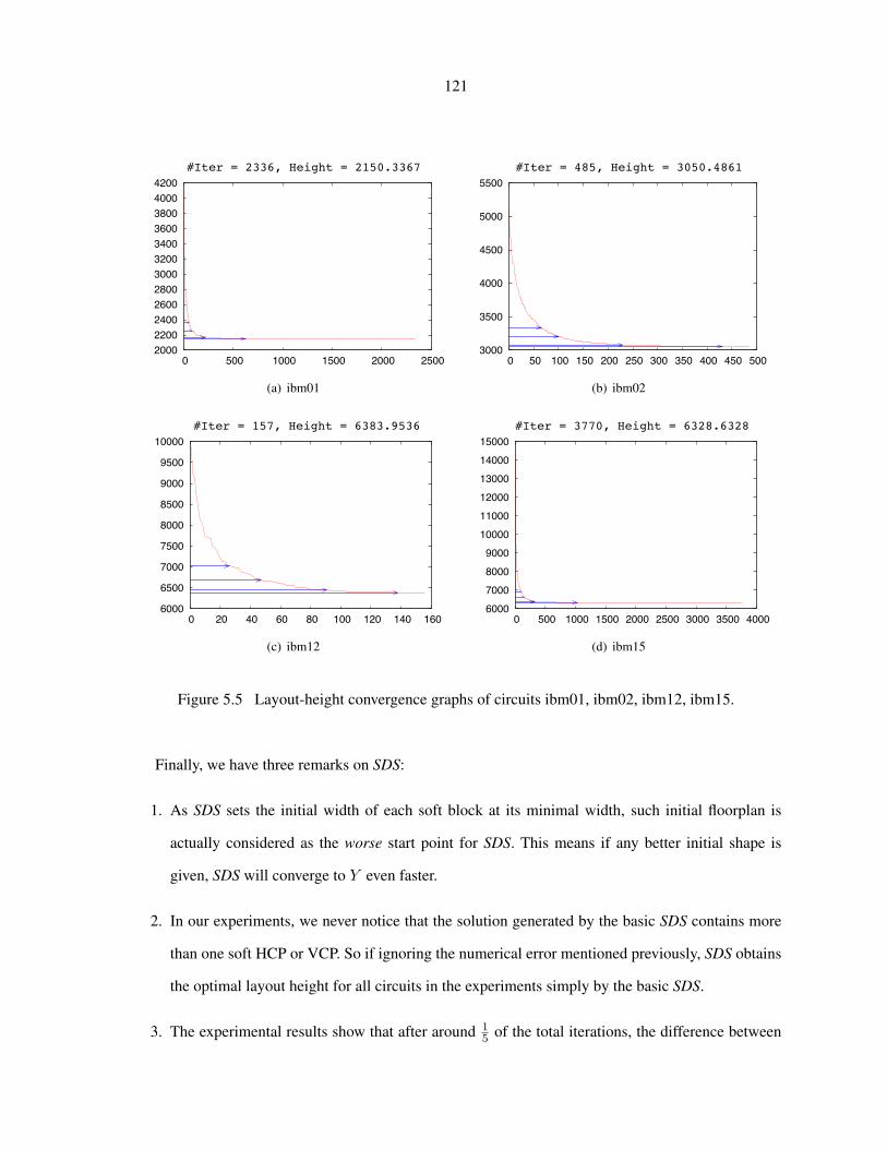
121
2000 2200 2400 2600 2800 3000 3200 3400 3600 3800 4000 4200
0 500 1000 1500 2000 2500
#Iter = 2336, Height = 2150.3367
(a) ibm01
3000
3500
4000
4500
5000
5500
0 50 100 150 200 250 300 350 400 450 500
#Iter = 485, Height = 3050.4861
(b) ibm02
6000
6500
7000
7500
8000
8500
9000
9500
10000
0 20 40 60 80 100 120 140 160
#Iter = 157, Height = 6383.9536
(c) ibm12
6000 7000 8000 9000
10000 11000 12000 13000 14000 15000
0 500 1000 1500 2000 2500 3000 3500 4000
#Iter = 3770, Height = 6328.6328
(d) ibm15
Figure 5.5 Layout-height convergence graphs of circuits ibm01, ibm02, ibm12, ibm15.
Finally, we have three remarks on SDS:
1. As SDS sets the initial width of each soft block at its minimal width, such initial floorplan is
actually considered as the worse start point for SDS. This means if any better initial shape is
given, SDS will converge to Y even faster.
2. In our experiments, we never notice that the solution generated by the basic SDS contains more
than one soft HCP or VCP. So if ignoring the numerical error mentioned previously, SDS obtains
the optimal layout height for all circuits in the experiments simply by the basic SDS.
3. The experimental results show that after around 15 of the total iterations, the difference between
122
yn+1 and Y is already considered quite small, i.e., less than 1%. So in practice if it is not
necessary to obtain an optimal solution, we can basically set a threshold value on the amount of
change on yn+1 as the stopping criterion. For example, if the amount of change on yn+1 is less
than 1% during the last 10 iterations, then SDS will stop.
5.7 Conclusion
In this chapter, we have proposed an efficient, scalable and optimal slack-driven shaping algorithm
for soft blocks in non-slice floorplan. Unlike previous work, we formulate the problem in a way, such
that it can be applied for fixed-outline floorplanning. For all cases in our experiments, the basic SDS is
sufficient to obtain an optimal solution. Both the efficiency and effectiveness of SDS have been validated
by comprehensive experimental results. In the future, we will modify SDS so that it can also be applied
for classical floorplanning. We also believe the slack-driven shaping algorithm can be modified and
applied on buffer/wire sizing in timing optimization.

123
CHAPTER 6 Geometry Constraint Aware Floorplan-Guided Placement
One never notices what has been done; one can only see what remains to be done.
— Marie Curie
6.1 Introduction
In Chapter 3, we present FLOP that can effectively handle large-scale mixed-side designs with all
movable objects. In this chapter, we propose several key techniques to be improve FLOP, and imple-
ment an ultimate geometry constraint aware floorplan-guided placer, namely FLOPC. The main focus of
these techniques is to enable an efficient annealing-based floorplanning framework to handle the geom-
etry constraints. To further improve the QoR of FLOPC, we apply SafeChoice as the stand-alone clus-
tering algorithm applied in the block formation step to cut down the problem size. Moreover, a min-cost
flow algorithm is used to substitute the linear programming formulation in the shifting step to speedup
the runtime. FLOPC can efficiently handle mixed-size designs with various geometry constraints, e.g.,
preplaced, range and boundary constraints, etc. To demonstrate the effectiveness of FLOPC, we derived
another version of Modern Mixed-Size (MMS) placement benchmarks with geometry constraints.
The rest of this chapter is organized as follows. Section 6.2 gives the overview of FLOPC. Sec-
tion 6.3 describes the enhanced annealing-based floorplanning framework. The experimental results are
presented in Section 6.4. Finally, this chapter ends with a conclusion in Section 6.5.
6.2 Overview of FLOPC
Essentially, FLOPC follows the same algorithm flow in Figure 1.3.

124
1. Block Formation: In this step, SafeChoice is first applied to cluster the small objects in the
circuit. To further cut down the problem size after clustering, we still perform partitioning on the
clustered netlist. At the end, small objects in each partition are clustered into a soft block and
each big macro becomes one single hard block.
2. Floorplanning: Different from FLOP, in this step we adopt an enhanced annealing-based floor-
planning framework. Due to the inherent slowness of annealing, we are not completely relying on
it to produce a good floorplan. Basically, we first apply DeFer to generate a floorplan containing
only the blocks without geometry constraints, i.e., non-constraint blocks. Secondly, we physically
insert the constraint blocks into this floorplan and obtain an initial legal floorplan containing all
blocks in the circuit. After such insertion, the constraint blocks are close to their locations spec-
ified in the geometry constraints, and most non-constraint blocks also maintain their previous
locations generated by DeFer. Thus, this initial floorplan gives the annealing-based floorplan-
ner a good start point. Finally, we apply the annealing process to further optimize the complete
block-level netlist with geometry constraint awareness, and output a final legal floorplan.
3. Wirelength-Driven Shifting: We use the min-cost flow based algorithm in [42] to substitute the
LP-based shifting process in FLOP. This significantly cuts down the runtime of the shifting step,
while obtaining the same optimal layout solution.
4. Incremental Placement: In the last step, we apply the same analytical placement algorithm as
in Figure 3.2 to further optimize the location of the small objects.
6.3 Enhanced Annealing-Based Floorplanning
In this section, we present the enhanced annealing-based floorplanning adopted in the floorplan-
ning step in FLOPC. We use the sequence pair to represent a floorplan layout in the annealing-based
framework. Let S(S+, S−) denote the sequence pair, where S+ is the positive sequence and S− is the
negative sequence. To model the geometry relationship among the blocks, the horizontal and vertical
constraint graphs are derived from a given sequence pair. In the constraint graph, the vertex represents
the block and the edge between two vertices represents the non-overlapping constraint between the two
125
corresponding blocks. Using the longest path algorithm, the block locations can be calculated from the
given constraint graphs.
The algorithm flow of the enhanced annealing-based floorplanning is shown in Figure 6.1. Comparing
this flow with the flow of traditional annealing-based floorplanner, the main difference is the generation
of initial floorplan. Rather than starting from a random initial floorplan, which the traditional approach
does, as shown in Figure 6.1 we start the annealing process based on an initial floorplan linit generated
from a high-quality sequence pair, i.e., Sinit. Sinit is produced by inserting the sequence pair containing
only constraint blocks (i.e., Sc) into the sequence pair containing only non-constraint blocks (i.e., Sc).
It is a high-quality sequence pair in the following two aspects:
• In the initial legal floorplan linit generated from Sinit, the constraint blocks are placed close to
the physical locations specified in the geometry constraints.
• The initial locations of non-constraint blocks are generated by the high-quality floorplanner De-
Fer with both wirelength and packing awareness. Although after insertion some of their locations
may be disturbed, most non-constraint blocks still hold their initial positions.
As a result, the initial floorplan linit gives the annealing process a much better solution to start with.
This significantly improves both the efficiency and quality of the annealing-based floorplanning. In
order to generate a high-quality initial sequence pair Sinit, we propose two key techniques: 1) A simple
and efficient sequence pair generation algorithm that produces a sequence pair from a given legal layout;
2) A location aware sequence pair insertion algorithm that inserts one sequence pair into another while
maintaining the block physical locations as much as possible. These two techniques are described in
the subsequent two subsections.
6.3.1 Sequence Pair Generation from Given Layout
Since the sequence pair representation was introduced in [71], a lot of previous work have been
focusing on efficiently generating a legal layout from a given sequence pair. Few algorithm has been
proposed to solve the problem of generating a sequence pair from a given legal layout. In [71], Murata
et al. used the Gridding method via drawing the up-right and down-left step-lines to derive a sequence

126
Generate sequence pair
Block-level netlist
Non-constraintblocks
Constraintblocks
DeFer Generate sequence pair
Optimized Legal Layout
Sc
Sc-
Insert intoSc Sc-
Sinit
Generate initial floorplan l init
Set initial temperature
Perturb floorplan l new
Accept ?
Continue at currenttemperature ?
= l newl
Reduce temperature
Cold enough ?
Final floorplan
Y N
Y
N
N
Y
Figure 6.1 Flow of enhanced annealing-based floorplanning.

127
bL R
U
B
UL UR
BL BR
Figure 6.2 Divided eight chip regions around block b.
pair from a layout. However, this method is not intuitive for implementation. In this subsection, we
propose a very simple and efficient O(n2) algorithm to solve this problem.
To construct a sequence pair S(S+, S−) from a given legal layout, we apply the following three
steps:
1. First, based on the physical location information in the layout, we determine the relative orders
of every two blocks in both S+ and S−.
2. Second, two directed acyclic graphsG+ andG− are constructed. InG+, each vertex corresponds
to a block in the design and each direct edge between two vertices represents the relative order of
the corresponding two blocks in S+. G− is constructed in a similar way for S−.
3. Finally, by applying topological sort on G+ and G−, we can generate S+ and S−, respectively.
In the following part, we use two blocks a and b as an example to demonstrate how to determine their
relative orders in S+ and S−.
In the layout, we divide the part of whole chip region, which is not occupied by block b, into the
following eight regions, left (L), right (R), upper (U ), bottom (B), upper-left (UL), upper-right (UR),
bottom-left (BL) and bottom-right (BR) regions (see Figure 6.2). Given another block a, there are
the following eight 1 possible location relations between a and b in the layout.
1. a is on the left of b, if a overlaps with L region.1Since the given layout is legal, a and b would not overlap with each other.

128
2. a is on the right of b, if a overlaps with R region.
3. a is above b, if a overlaps with U region.
4. a is below b, if a overlaps with B region.
5. a is on the left of and above b, if a only overlaps with UL region.
6. a is on the right of and above b, if a only overlaps with UR region.
7. a is on the left of and below b, if a only overlaps with BL region.
8. a is on the right of and below b, if a only overlaps with BR region.
As we know, a sequence pair S(S+, S−) containing a and b imposes the following horizontal and
vertical relations between a and b in the layout:
• Horizontal Relation
If a is before b in S+ and before b in S−, a is on the left of b in the layout.
If a is after b in S+ and after b in S−, a is on the right of b in the layout.
• Vertical Relation
If a is after b in S+ and before b in S−, a is below b in the layout.
If a is before b in S+ and after b in S−, a is above b in the layout.
Based on the above statements, if the horizontal and vertical relations between a and b are known, we
can trace back to the sequence pair and find out their relative orders in S+ and S−. Therefore, for the
eight possible location relations mentioned previously, their corresponding relative orders between a
and b in S+ and S− are determined as follows.
1. If a is on the left of b, a is before b in S+ and before b in S−.
2. If a is on the right of b, a is after b in S+ and after b in S−.
3. If a is above b, a is before b in S+ and after b in S−.
4. If a is below b, a is after b in S+ and before b in S−.

129
5. If a is on the left of and above b, a is before b in S+.
6. If a is on the right of and above b, a is after b in S−
7. If a is on the left of and below b, a is before b in S−.
8. If a is on the right of and below b, a is after b in S+.
Using the above eight conditions, we can determine the relative order of any two blocks in S.
Now we construct two directed acyclic graphs G+ and G− to capture the relative order information
for every pair of blocks in S+ and S−. For example, G+ can be build up in the following manner. Each
vertex in G+ represents a block in the design. Given any two blocks a and b, if a is before b in S+,
then a direct edge from a to b is added; if a is after b in S+, then a direct edge from b to a is added;
otherwise, no edge is added between a and b. G− can be build up in the similar manner for every pair
of blocks in S−.
Finally, we apply topological sort on these two graphs G+ and G−. After sorting, the resulted
sequences from G+ and G− are basically S+ and S−, respectively.
As you can see, the process of sequence pair generation takesO(n2) time, as we traverse every pair
of blocks in the design. Nevertheless, sometimes it is not necessary consider every pair of blocks. For
example, given three blocks a, b and c, in the layout if a is on the left of b and b is on the left of c, it is
certain that a is on the left of c, which means we do not need to consider the relative order between a and
c in both S+ and S−. In order to capture such transitive relation, more sophisticated data structure is
needed, and thus potentially the algorithm complexity can be cut down to O(n log n). Because during
the whole annealing flow in Figure 6.1 we only apply the sequence pair generation technique twice,
i.e., generating Sc and Sc, the potential runtime improvement from O(n2) to O(n log n) would not be
significant.
6.3.2 Sequence Pair Insertion with Location Awareness
In Figure 6.1, two sequence pairs Sc and Sc are combined to generate Sinit that contains all blocks in
the design, such that the following two goals are achieved: 1) The locations of constraint blocks in linit
should be close to the locations specified in the geometry constraints; 2) The locations of non-constraint

130
blocks in linit should be close to the locations generated by DeFer in the previous step. To achieve these
two goals, in this subsection we propose a location aware sequence pair insertion technique that inserts
Sc(S+c , S
−c ) into Sc(S+
c , S−c ). The resulted sequence pair after the insertion is Sinit.
Practically, the constraint block can be inserted at any position in the sequence pair. However, in
order to produce minimal disturbance on the original block locations, it is obvious that during the inser-
tion the relative orders of blocks in both Sc and Sc should not be changed. Moreover, for each constraint
block there should be a corresponding range of the possible insertion positions in the sequence pair. We
call such range insertion range. For each block to be inserted, the insertion range specifies the left-most
and right-most possible insertion positions in the sequence pair.
The main idea of the insertion technique we propose is to use block packing to find the insertion
range in both S+c and S−c for each constraint block. For example, given a constraint block i, we want to
find its right-most insertion position in S−c . Based on the horizontal and vertical relations imposed by
the sequence pair, the blocks before i in S−c should be either on the left or below i in the layout. Thus,
we traverse the blocks in S−c from left to right and pack them one by one to the bottom-left corner of the
chip region, until we find any block in S−c , say block j, is neither on the left nor below i. This means
block j has to be after block i in S−c . Thus, the position before block j in S−c is basically the right-most
insertion position for block i.
Before we present the detailed algorithm of calculating the insertion range in S+c and S−c , we first
introduce some notations. Let Cul, Cur, Cbl and Cbr denote the upper-left, upper-right, bottom-left, and
bottom-right corners of the chip region, respectively. Assuming the index of the non-constraint blocks
are 1, 2, . . . ,m, and index of the constraint blocks are 1, 2, . . . , n. Let S+[i] denote the index of the
block at the ith position in S+, similarly we can define S−[i]. We define (L+i , R
+i ) as the insertion
range in S+c for block i, where L+
i and R+i denote the left-most and right-most insertion positions,
respectively. Similarly, the insertion range in S−c for block i is defined as (L−i , R−i ).
The pseudocode of calculating the insertion range in S+c and S−c are shown in Figure 6.3 and 6.4,
respectively. Before calculating the insertion range, it is first initialized as spanning the whole sequence,
i.e., the left-most and right-most insertion positions are the start and end position of the final sequence,
respectively. This initial range is considered to be loose, which basically implies the constraint block
131
can be inserted at any position. As the algorithm moves forward, a tighter range will be determined
based on packing. After the insertion range is determined for each constraint block, the middle position
between the left-most and right-most insertion positions is used as the final insertion position.
6.3.3 Constraint Handling and Annealing Schedule
Essentially, we adopt a similar annealing-based method as in [72] to handle various geometry con-
straints. Specifically, in FLOPC we consider the following three kinds of geometry constraints:
• Preplaced Constraint: This constraint is imposed, when some block has to be preplaced and
fixed at some location in the chip region.
• Range Constraint: This constraint specifies that some block has to be within a certain coordi-
nates range in either horizontal or vertical direction. If both horizontal and vertical range con-
straints are imposed on the same block, then this constraint is the same as region constraint.
• Boundary Constraint: This constraint specifies that some block has to be placed along either
one of the four boundaries of the chip region.
The above three geometry constraints are the most commonly considered ones in modern mixed-size
placement. Based on the framework proposed in [72], FLOPC can be easily extended to handle other
geometry constraints.
As shown in Figure 6.1, after the initial floorplan linit is generated, we apply the annealing process to
optimize both the total HPWL and packing among the blocks, while satisfying the geometry constraints.
Therefore, the following cost function is used to evaluate a floorplan in annealing.
C = W + αPo + βPc
In the above cost function, W is the term of average HPWL over all nets in the block-level netlist, Po
is the penalty term if the blocks are placed outside of the chip region, and Pc is the penalty term for the
geometry constraints. α and β are the weight among the three terms (by default, α = 2 and β = 4). In
each annealing iteration we first apply one of the following four moves to change the existing floorplan
l.
132
• Switch two random blocks in one sequence pair
• Rotate random hard blocks
• Switch two random blocks on the horizontal or vertical critical path
• Rotate random hard bocks on the horizontal or vertical critical path
To shape the soft blocks in the floorplan, we use the shaping algorithm SDS proposed in Chapter 5.
Because SDS is always applied on some existing floorplan where the soft blocks have reasonably good
shape, we do not need to stop SDS until it converges. We basically run at most γ iterations of shaping
inside each annealing iteration (γ = 100 by default). The output of SDS is the new floorplan lnew
obtained. Then we will compare the cost between lnew and l to determine whether we should accept
this move or not.
6.4 Experimental Results
In this section, we first describe the construction of the MMS benchmarks with geometry con-
straints. Then we present the experimental results of FLOPC on this new set of benchmarks. All
experiments are run on a Linux server with AMD Opteron 2.59 GHz CPU and 16GB memory.
In Chapter 3, we construct the Modern Mixed-Size (MMS) placement benchmarks based on ISPD05/06
benchmarks. But, in MMS benchmarks all objects are movable except the I/O objects. In order to show
the effectiveness of FLOPC, for each circuit in MMS benchmarks we add some geometry constraints
on some hard macros. Basically, we add three kinds of geometry constraints, preplaced, range and
boundary constraints. The list of various geometry constraints in each circuit is shown in Table 6.1.
The experimental results on MMS benchmarks with geometry constraints are shown in Table 6.2.
It is clear that FLOPC is able to efficiently and successfully satisfy all geometry constraints on all 16
circuits. As all other mixed-size placers can only handle preplaced constraints, we can only compare
with them on 6 circuits. Basically, we compare FLOPC with mPL6 and Capo10.5. Even for the
circuit with only preplaced constraints, it is still every difficult for mPL6 and Capo10.5 to produce
a legal solution. For example, mPL6 failed to generate a legal solution on 4 circuits. On average,

133
Table 6.1 List of geometry constraints in Modern Mixed-Size placement benchmarks.
Geometry ConstraintsCircuit #. Preplaced #. Range #. Boundary Total #.
Constraints Constraints Constraints Constraintsadaptec1 4 - - 4adaptec2 2 1 - 3adaptec3 6 - - 6adaptec4 1 1 1 3bigblue1 2 5 3 10bigblue2 4 - - 4bigblue3 2 6 - 8bigblue4 4 - - 4adaptec5 2 - - 2newblue1 1 2 - 3newblue2 - - 8 8newblue3 - - 18 18newblue4 2 4 4 10newblue5 4 - - 4newblue6 - 8 - 8newblue7 - 8 - 8
FLOPC generates 1% and 8% of better wirelength than mPL6 and Capo10.5 respectively. Regarding
the runtime, FLOPC is 7× and 6% faster than Capo10.5 and mPL6 respectively.
6.5 Conclusion
Based on the algorithm flow of FLOP, in this chapter we have presented FLOPC that can efficiently
handle large-scale mixed-size designs with various geometry constraints. FLOPC adopts an annealing-
based floorplanning framework to handle various geometry constraints. Several key techniques are
proposed to improve the efficiency of such annealing-based framework. Promising experimental results
are shown to demonstrate the effectiveness of FLOPC. Such high-quality and effective placement tool
is expected to handle the challenges and complexities of modern large-scale mixed-size placements.

134
Table 6.2 Comparison with mixed-size placers on MMS benchmarks with constraints (* circuit withonly preplaced constraints).
Circuit mPL6[6] Capo10.5[2] FLOPCHPWL (×10e6) Time (s) HPWL (×10e6) Time (s) HPWL (×10e6) Time (s)
adaptec1* 99.28 2410 100.13 4988 98.11 2267adaptec2 – – – – 159.38 1021
adaptec3* illegal – 252.64 15322 207.56 2093adaptec4 – – – – 195.14 1572bigblue1 – – – – 103.37 1209
bigblue2* illegal – illegal – 167.80 4360bigblue3 – – – – 540.14 8101
bigblue4* illegal – 912.72 102460 SEGV SEGVadaptec5* illegal – 385.86 34277 355.05 4170newblue1 – – – – 80.75 1862newblue2 – – – – 342.25 5887newblue3 – – – – 552.90 3482newblue4 – – – – 250.33 2501
newblue5* illegal – 550.69 66594 546.80 7454newblue6 – – – – 531.02 13177newblue7 – – – – 2178.60 9075
Norm 1.01 1.06 1.08 6.67 1 1
Begin1. Initialize L+
i = 1, 1 ≤ i ≤ n2. k = n.3. For j = m to 14. b = S+
c [j].5. Pack block b to Cbr.6. For i = k to 17. bc = S+
c [i].8. If b is neither on the right of nor below bc,9. L+
bc= j + 1.
10. k = k − 1.11. j = j + 1.12. Break.End
(a) Left-most insertion position calculation
Begin1. Initialize R+
i = m+ n, 1 ≤ i ≤ n2. k = n.3. For j = 1 to m4. b = S+
c [j].5. Pack block b to Cul.6. For i = 1 to k7. bc = S+
c [i].8. If b is neither on the left of nor above bc,9. R+
bc= j − 1.
10. k = k + 1.11. j = j − 1.12. Break.End
(b) Right-most insertion position calculation
Figure 6.3 Calculation of insertion range in S+c .

135
Begin1. Initialize L−i = 1, 1 ≤ i ≤ n2. k = n.3. For j = m to 14. b = S−c [j].5. Pack block b to Cur.6. For i = k to 17. bc = S−c [i].8. If b is neither on the right of nor above bc,9. L−bc = j + 1.10. k = k − 1.11. j = j + 1.12. Break.End
(a) Left-most insertion position calculation
Begin1. Initialize R−i = m+ n, 1 ≤ i ≤ n2. k = n.3. For j = 1 to m4. b = S−c [j]5. Pack block b to Cbl.6. For i = 1 to k7. bc = S−c [i].8. If b is neither on the left of nor below bc,9. R−bc = j − 1.10. k = k + 1.11. j = j − 1.12. Break.End
(b) Right-most insertion position calculation
Figure 6.4 Calculation of insertion range in S−c .

136
BIBLIOGRAPHY
[1] T. Taghavi, X. Yang, B.-K. Choi, M. Yang, and M. Sarrafzadeh. Dragon2006: Blockage-aware
congestion-controlling mixed-size placer. In Proc. ISPD, pages 209–211, 2006.
[2] J. A. Roy, S. N. Adya, D. A. Papa, and I. L. Markov. Min-cut floorplacement. IEEE Trans. on
Computer-Aided Design, 25(7):1313–1326, July 2006.
[3] N. Viswanathan, M. Pan, and C. Chu. Fastplace 3.0: A fast multilevel quadratic placement algo-
rithm with placement congestion control. In Proc. ASP-DAC, pages 135–140, 2007.
[4] A. B. Kahng and Q. Wang. A faster implementation of APlace. In Proc. ISPD, pages 218–220,
2006.
[5] P. Spindler, U. Schlichtmann, and F. M. Johannes. Kraftwerk2 – A fast force-directed quadratic
placement approach using an accurate net model. IEEE Trans. on Computer-Aided Design,
27(8):1398–1411, August 2008.
[6] T. Chan, J. Cong, J. Shinnerl, K. Sze, and M. Xie. mPL6: Enhanced multilevel mixed-sized
placement. In Proc. ISPD, pages 212–214, 2006.
[7] T.-C. Chen, Z.-W. Jiang, T.-C. Hsu, H.-C. Chen, and Y.-W. Chang. A high-quality mixed-size
analytical placer considering preplaced blocks and density constraints. In Proc. ICCAD, pages
187–192, 2006.
[8] T.-C. Chen, P.-H. Yuh, Y.-W. Chang, F.-J. Huang, and D. Liu. MP-tree: A packing-based macro
placement algorithm for mixed-size designs. In Proc. DAC, pages 447–452, 2007.
[9] H.-C. Chen, Y.-L. Chuang, Y.-W. Chang, and Y.-C. Chang. Constraint graph-based macro place-
ment for modern mixed-size circuit designs. In Proc. ICCAD, pages 218–223, 2008.

137
[10] S. Adya and I. Markov. Consistent placement of macro-blocks using floorplanning and standard-
cell placement. In Proc. ISPD, pages 12–17, 2002.
[11] J. Z. Yan and C. Chu. DeFer: Deferred decision making enabled fixed-outline floorplanner. In
Proc. DAC, pages 161–166, 2008.
[12] J. Z. Yan and C. Chu. DeFer: Deferred decision making enabled fixed-outline floorplanning
algorithm. IEEE Trans. on Computer-Aided Design, 43(3):367–381, March 2010.
[13] J. Z. Yan, N. Viswanathan, and C. Chu. Handling complexities in modern large-scale mixed-size
placement. In Proc. DAC, pages 436–441, 2009.
[14] J. Z. Yan, C. Chu, and W. K. Mak. SafeChoice: A novel clustering algorithm for wirelength-driven
placement. In Proc. ISPD, pages 185–192, 2010.
[15] J. Z. Yan, C. Chu, and W. K. Mak. SafeChoice: A novel approach to hypergraph clustering for
wirelength-driven placement. IEEE Trans. on Computer-Aided Design, 30(7), July 2011.
[16] J. Z. Yan and C. Chu. Optimal slack-driven block shaping algorithm in fixed-outline floorplanning.
submitted to ICCAD 2011.
[17] A. B. Kahng. Classical floorplanning harmful? In Proc. ISPD, pages 207–213, 2000.
[18] R. H. J. M. Otten. Efficient floorplan optimization. In Proc. ICCD, pages 499–502, 1983.
[19] S. N. Adya and I. L. Markov. Fixed-outline floorplanning through better local search. In Proc.
ICCD, pages 328–334, 2001.
[20] S. N. Adya and I. L. Markov. Fixed-outline floorplanning: Enabling hierarchical design. IEEE
Trans. on VLSI Systems, 11(6):1120–1135, December 2003.
[21] T.-C. Chen and Y.-W. Chang. Modern floorplanning based on B*-trees and fast simulated anneal-
ing. IEEE Trans. on Computer-Aided Design, 25(4):637–650, April 2006.
[22] Y. C. Wang, Y. W. Chang, G. M. Wu, and S. W. Wu. B*-Tree: A new representation for non-slicing
floorplans. In Proc. DAC, pages 458–463, 2000.

138
[23] T.-C. Chen, Y.-W. Chang, and S.-C. Lin. A new multilevel framework for large-scale interconnect-
driven floorplanning. IEEE Trans. on Computer-Aided Design, 27(2):286–294, February 2008.
[24] S. Chen and T. Yosihmura. Fixed-outline floorplanning: Enumerating block positions and a new
objective function for calculating area costs. IEEE Trans. on Computer-Aided Design, 27(5):858–
871, May 2008.
[25] O. He, S. Dong, J. Bian, S. Goto, and C.-K. Cheng. A novel fixed-outline floorplanner with zero
deadspace for hierarchical design. In Proc. ICCAD, pages 16–23, 2008.
[26] A. Ranjan, K. Bazargan, S. Ogrenci, and M. Sarrafzadeh. Fast floorplanning for effective predic-
tion and construction. IEEE Trans. on VLSI Systems, 9(2):341–352, April 2001.
[27] P. G. Sassone and S. K. Lim. A novel geometric algorithm for fast wire-optimized floorplanning.
In Proc. ICCAD, pages 74–80, 2003.
[28] Y. Zhan, Y. Feng, and S. S. Sapatnekar. A fixed-die floorplanning algorithm using an analytical
approach. In Proc. ASP-DAC, pages 771–776, 2006.
[29] J. Cong, M. Romesis, and J. R. Shinnerl. Fast floorplanning by look-ahead enabled recursive
bipartitioning. IEEE Trans. on Computer-Aided Design, 25(9):1719–1732, September 2006.
[30] M. Lai and D. F. Wong. Slicing tree is a complete floorplan representation. In Proc. DATE, pages
228–232, 2001.
[31] L. Stockmeyer. Optimal orientations of cells in slicing floorplan designs. Information and Control,
57:91–101, May/June 1983.
[32] G. Zimmermann. A new area and shape function estimation technique for VLSI layouts. In Proc.
DAC, pages 60–65, 1988.
[33] A. E. Dunlop and B. W. Kernighan. A procedure for placement of standard-cell VLSI circuits.
IEEE Trans. on Computer-Aided Design, 4(1):92–98, January 1985.
[34] G. Karypis and V. Kumar. Multilevel k-way hypergraph partitioning. In Proc. DAC, pages 343–
348, 1999.

139
[35] S. Goto. An efficient algorithm for the two-dimensional placement problem in electrical circuit
layout. IEEE Trans. on Circuits and Systems, CAS-28(1):12–18, January 1981.
[36] GSRC floorplan benchmarks.
http://vlsicad.eecs.umich.edu/BK/GSRCbench/.
[37] HB floorplan benchmarks.
http://cadlab.cs.ucla.edu/cpmo/HBsuite.html.
[38] A. Ng, I. L. Markov, R. Aggarwai, and V. Ramachandran. Solving hard instances of floorplace-
ment. In Proc. ISPD, pages 170–177, 2006.
[39] Source Code and Benchmarks Download.
http://www.public.iastate.edu/˜zijunyan/.
[40] G.-J. Nam, C. J. Alpert, P. Villarrubia, B. Winter, and M. Yildiz. The ISPD2005 placement contest
and benchmarks suite. In Proc. ISPD, pages 216–220, 2005.
[41] G.-J. Nam. ISPD 2006 placement contest: Benchmark suite and results. In Proc. ISPD, pages
167–167, 2006.
[42] X. Tang, R. Tian, and M. D. F. Wong. Minimizing wire length in floorplanning. IEEE Trans. on
Computer-Aided Design, 25(9):1744–1753, September 2006.
[43] P.-N. Guo, C.-K. Cheng, and T. Yoshimura. An O-tree representation of non-slicing floorplan and
its applications. In Proc. DAC, pages 268–273, 1999.
[44] G.-J. Nam, S. Reda, C. J. Alpert, P. G. Villarrubia, and A. B. Kahng. A fast hierarchical quadratic
placement algorithm. IEEE Trans. on Computer-Aided Design, 25(4):678–691, April 2006.
[45] M. Pan, N. Viswanathan, and C. Chu. An efficient and effective detailed placement algorithm. In
Proc. ICCAD, pages 48–55, 2005.
[46] S. Adya, S. Chaturvedi, J. Roy, D. Papa, and I. Markov. Unification of partitioning, placement and
floorplanning. In Proc. ICCAD, pages 550–557, 2004.

140
[47] hMetis2.0.
http://glaros.dtc.umn.edu/gkhome/.
[48] QSopt LP Solver.
http://www.isye.gatech.edu/˜wcook/qsopt/.
[49] P. Spindler and F. M. Johannes. Fast and robust quadratic placement combined with an exact linear
net model. In Proc. ICCAD, pages 179–186, 2006.
[50] J. Cong and M. Xie. A robust detailed placement for mixed-size IC designs. In Proc. ASP-DAC,
pages 188–194, 2006.
[51] B. Hu and M. Marek-Sadowska. Multilevel fixed-point-addition-based VLSI placement. IEEE
Trans. on Computer-Aided Design, 24(8):1188–1203, August 2005.
[52] N. Viswanathan, G.-J. Nam, C. Alpert, P. Villarrubia, H. Ren, and C. Chu. RQL: Global placement
via relaxed quadratic spreading and linearization. In Proc. DAC, pages 453–458, 2007.
[53] C. J. Alpert and A. B. Kahng. Recent developments in netlist partitioning: A survey. Integration,
the VLSI Journal, 19(1-2):1–81, August 1995.
[54] G. Karypis, R. Aggarwal, V. Kumar, and S. Shekhar. Multilevel hypergraph partitioning: Appli-
cation in VLSI domain. In Proc. DAC, pages 526–529, 1997.
[55] C. J. Alpert, J.-H. Huang, and A. B. Kahng. Multilevel k-way hypergraph partitioning. In Proc.
DAC, pages 530–533, 1997.
[56] T. Chan, J. Cong, and K. Sze. Multilevel generalized force-directed method for circuit placement.
In Proc. ISPD, pages 185–192, 2005.
[57] J. Cong and S. K. Lim. Edge separability-based circuit clustering with application to multilevel
circuit partitioning. IEEE Trans. on Computer-Aided Design, 23(3):346–357, March 2004.
[58] B. Hu and M. Marek-Sadowska. Fine granularity clustering-based placement. IEEE Trans. on
Computer-Aided Design, 23(4):527–536, April 2004.

141
[59] G.-J. Nam, S. Reda, C. J. Alpert, P. G. Villarrubia, and A. B. Kahng. A fast hierarchical quadratic
placement algorithm. IEEE Trans. on Computer-Aided Design, 25(4):678–691, April 2006.
[60] J. Li, L. Behjat, and J. Huang. An effective clustering algorithm for mixed-size placement. In
Proc. ISPD, pages 111–118, 2007.
[61] C. M. Fiduccia and R. M. Mattheyses. A linear-time heuristic for improving network partitions.
In Proc. DAC, pages 175–181, 1982.
[62] H. Chen, C.-K. Cheng, N.-C. Chou, A. B. Kahng, J. F. MacDonald, P. Suaris, B. Yao, and Z. Zhu.
An algebraic multigrid solver for analytical placement with layout based clustering. In Proc. DAC,
pages 794–799, 2003.
[63] P. Pan and C. L. Liu. Area minimization for floorplans. IEEE Trans. on Computer-Aided Design,
14(1):129–132, January 1995.
[64] T. C. Wang and D. F. Wong. Optimal floorplan area optimization. IEEE Trans. on Computer-Aided
Design, 11(8):992–1001, August 1992.
[65] M. Kang and W. W. M. Dai. General floorplanning with L-shaped, T-shaped and soft blocks based
on bounded slicing grid structure. In Proc. ASP-DAC, pages 265–270, 1997.
[66] S. Nakatake, K. Fujiyoshi, H. Murata, and Y. Kajitani. Module placement on BSG-structure and
IC layout applications. In Proc. ICCAD, pages 484–491, 1996.
[67] T. S. Moh, T. S. Chang, and S. L. Hakimi. Globally optimal floorplanning for a layout problem.
IEEE Trans. on Circuits and Systems I, 43:713–720, September 1996.
[68] H. Murata and E. S. Kuh. Sequence-pair based placement method for hard/soft/pre-placed mod-
ules. In Proc. ISPD, pages 167–172, 1998.
[69] F. Y. Young, C. C. N. Chu, W. S. Luk, and Y. C. Wong. Handling soft modules in general
non-slicing floorplan using Lagrangian relaxation. IEEE Trans. on Computer-Aided Design,
20(5):687–692, May 2001.

142
[70] C. Lin, H. Zhou, and C. Chu. A revisit to floorplan optimization by Lagrangian relaxation. In
Proc. ICCAD, pages 164–171, 2006.
[71] H. Murata, K. Fujiyoshi, S. Nakatake, and Y. Kajitani. VLSI module placement based on
rectangle-packing by the sequence-pair. IEEE Trans. on Computer-Aided Design, 15(12):1518–
1524, December 1996.
[72] E. F. Y. Young, C. C. N. Chu, and M. L. Ho. Placement constraints in floorplan design. IEEE
Trans. on VLSI Systems, 12(7):735–745, July 2004.
Recommended