Fall 2013 Biostat 511 1
(Biostatistics 511)
Week 7 Discussion Section
Lisa Brown
Medical Biometry I

Fall 2013 Biostat 511 2
The Normal Distribution
Many “Real world” measurements, such as IQ and height can be modeled was normal random variables (RVs).
Some RVs can have distributions that are approximately normal (provided certain conditions apply)• Binomial(n, p) • Poisson(l)
The central limit theorem: with large enough sample size, the distribution of sample means and sample proportions are approximately normal.

Fall 2013 Biostat 511 3
Skills and Concepts• The standard normal distribution and z-scores
• Finding probabilities
• Finding quantiles, given probabilties
• Word problems
• Using the normal approximation of the binomial distribution.
• Distribution of sample means and the central limit theorem
• Forming Confidence intervals for population means

Fall 2013 Biostat 511 4
The normal distribution or “bell-shaped” curve has two parameters.
• = the mean of X• = the standard deviation of X
Normal Distribution
• Notation: X ~ N(, )
• Cumulative distribution function (CDF) : P(X< c)
• Standard normal distribution Z ~ N(0,1)
P(Z<1.65)
Fall 2013 Biostat 511 5
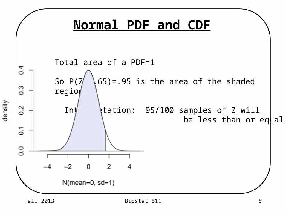
Normal PDF and CDF
Total area of a PDF=1
So P(Z<1.65)=.95 is the area of the shaded region.
Interpretation: 95/100 samples of Z will be less than or equal to 1.65

Fall 2013 Biostat 511 6
Obtaining values of standard normal CDF P(Z<c)
STATA: disp normal(1.65).95052853
Or use normal probability tables (e.g. back of Baldi and Moore)

Fall 2013 Biostat 511 7
We want:P(Z<1.65)

Fall 2013 Biostat 511 8
Probability rules: complementary events
= 1-
P(Z>1.65)=1-P(Z<1.65)=1-.95=.05

Fall 2013 Biostat 511 9
Symmetry property of standard normal RVs
=
P(Z<-1.65)=P(Z>1.65)=.05

Fall 2013 Biostat 511 10
Probabilities of intervals
=
P(-1.65<Z<1.65)=P(Z<1.65) - P(Z<-1.65) = .95-.05=.90For a standard normal RV, 90% of values fall between -1.65 and 1.65
-

Fall 2013 Biostat 511 11
P[Z < 1.65] = 0.9505
P[Z > 0.5] = 1-P[Z < 0.5] = 0.3085
P[-1.96 < Z < 1.96] = P[Z < 1.96] - P[Z < -1.96] = .95
P[-0.50 < Z < 2.0] = P[Z < 2.0] - P[Z < -0.50]
Standard Normal Probabilities: more practice
-0.50 2.0 -0.502.0
Why?
Fall 2013 Biostat 511 12
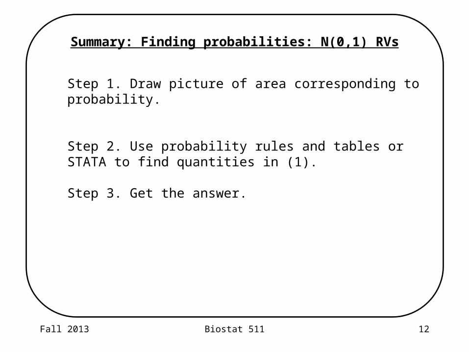
Step 1. Draw picture of area corresponding to probability.
Step 2. Use probability rules and tables or STATA to find quantities in (1).
Step 3. Get the answer.
Summary: Finding probabilities: N(0,1) RVs

Fall 2013 Biostat 511 13
Q: This solves the problem for the N(0,1) case. How do we do calculate normal probabilities when the mean is not 0 and the standard deviation is not equal to 1?
A: Any normal random variable can be transformed to N(0,1)
E(X- ) = 0
V(X- ) = V(X) = 2
V( (X- )/ ) =(1/2)*V(X)=1
Linear transformations of normal random variables are still normal. So
Z = (X-m)/s ~ N ( 0 , 1 )
Converting to Standard Normal: Z scores
Fall 2013 Biostat 511 14
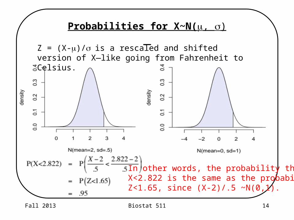
Probabilities for X~N(, )
Z = (X-m)/ s is a rescaled and shifted version of X—like going from Fahrenheit to Celsius.
In other words, the probability thatX<2.822 is the same as the probability Z<1.65, since (X-2)/.5 ~N(0,1).

Fall 2013 Biostat 511 15
Step 0. Draw picture of area corresponding to probability.
Step 1. Re-express probability statement about X as statement about Z by standardizing.
Step 2. Use probability rules and tables or STATA to find quantities in (1).
Step 3. Get the answer.
Summary: Finding probabilities: X~N( ,m s) RVs
Fall 2013 Biostat 511 16
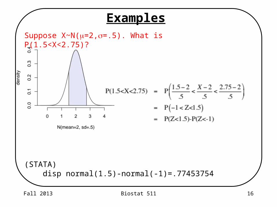
ExamplesSuppose X~N(m=2,s=.5). What is P(1.5<X<2.75)?
(STATA) disp normal(1.5)-normal(-1)=.77453754

Fall 2013 Biostat 511 17
Define the random variable in words.
Is it normally distributed? What is the mean and standard deviation?
What is the event and corresponding probability statement?
Draw picture of area corresponding to probability.
Re-express probability statement about X as statement about Z by standardizing.
Use probability rules and tables or STATA to find probabilities.
Get the answer.
Word Problems: approach

Fall 2013 Biostat 511 18
Suppose a clinically accepted value for mean systolic blood pressure in females, aged 65-74 is 133 mmHg and the standard deviation is 20 mmHg. If a 70-year-old- woman is selected at random from the population, what is the probability that her systolic blood pressure is equal to or less than 120 mmHg?
X = systolic BP in woman age 65-74.
= 133
= 20
What is P(X< 133)?
Word problem: BP in older women

Fall 2013 Biostat 511 19
Example Suppose a clinically accepted value for mean systolic blood pressure in females, aged 65-74 is 133 mmHg and the standard deviation is 20 mmHg. If a 70-year-old- woman is selected at random from the population, what is the probability that her systolic blood pressure is equal to or less than 120 mmHg?
STATA: display normal(-0.65)
Systolic BP

Fall 2013 Biostat 511 20
Normal quantiles
P(Z<1.65)=.95
The .95 quantile of a standard normal RV, z.95, is 1.65.
In general, P(Z<zp)=p

Fall 2013 Biostat 511 21
Normal quantiles: example
Suppose Z~N(0,1).
What is the .8 quantile (or 80th percentile) of Z?
P(Z<z.80)=.8
STATA: display invnorm(.8)
.84162123
Interpretation: There is an 80% chance that a randomly chosen Z~N(0,1)will fall below .84.

Fall 2013 Biostat 511 22
Normal quantiles: tables
P(Z<z.80)=.8…Find values of z with p closest to .8
From the table, P(Z<.84)=.7995 and P(Z<.85)=.8023So the .8th quantile is approximately .845.
Fall 2013 Biostat 511 23
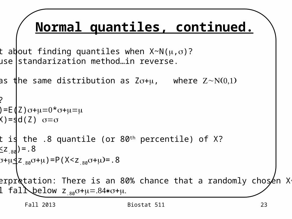
Normal quantiles, continued.
What about finding quantiles when X~N(m,s)?We use standarization method…in reverse.
X has the same distribution as Z +s m, where ~ (0,1)Z N
Why? E(Z)=E(Z) + =0s m * + =s m msd(X)=sd(Z) =s s
What is the .8 quantile (or 80th percentile) of X?P(Z<z.80)=.8P(Z +s m<z.80 +s m)=P(X<z.80 + )s m =.8
Interpretation: There is an 80% chance that a randomly chosen X~N(m,s)will fall below z.80 + =.84* + .s m s m
Fall 2013 Biostat 511 24
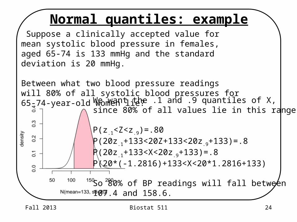
Normal quantiles: example Suppose a clinically accepted value for mean systolic blood pressure in females, aged 65-74 is 133 mmHg and the standard deviation is 20 mmHg.
Between what two blood pressure readings will 80% of all systolic blood pressures for 65-74-year-old women lie?
We want the .1 and .9 quantiles of X, since 80% of all values lie in this range.
P(z.1<Z<z.9)=.80P(20z.1+133<20Z+133<20z.9+133)=.8P(20z.1+133<X<20z.9+133)=.8P(20*(-1.2816)+133<X<20*1.2816+133)
So 80% of BP readings will fall between107.4 and 158.6.
Fall 2013 Biostat 511 25
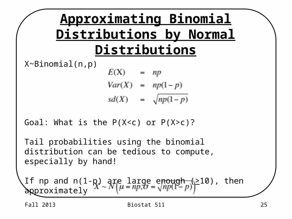
Approximating Binomial Distributions by Normal Distributions
X~Binomial(n,p)
Goal: What is the P(X<c) or P(X>c)?
Tail probabilities using the binomial distribution can be tedious to compute, especially by hand!
If np and n(1-p) are large enough (>10), then approximately

Fall 2013 Biostat 511 26
Example If np and n(1-p) are large enough (>10), then approximately
X~Binomial(n=200, p=.4). What is P(X<70)?
200*.4>10 and 200*.6>10, so, approximately
Exact calculation P(X<70)=.0843 STATA disp binomial(20,12,.5)
Fall 2013 Biostat 511 27
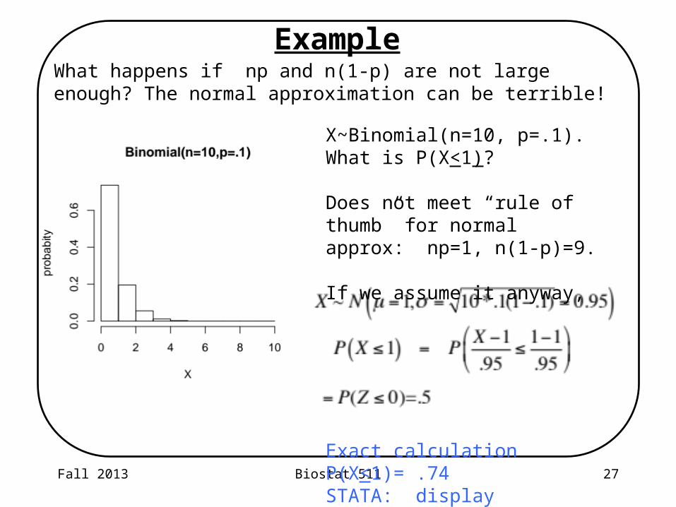
Example What happens if np and n(1-p) are not large enough? The normal approximation can be terrible!
X~Binomial(n=10, p=.1). What is P(X<1)?
Does not meet “rule of thumb” for normal approx: np=1, n(1-p)=9.
If we assume it anyway,
Exact calculation P(X<1)= .74STATA: display binomial(10,1,.1)

Fall 2013 Biostat 511 28
Sampling distribution of meansAssume that X1, X2,...,Xn are an independent, identically distributed sample of RVsfrom a distribution with mean m and variance s2 (sd ) .s
The sample mean is another random variable
So as n gets, bigger, the standard deviation of the sample mean goes down. If sd(X) =10, what is the sd of the the sample mean when n=100?
Fall 2013 Biostat 511 29
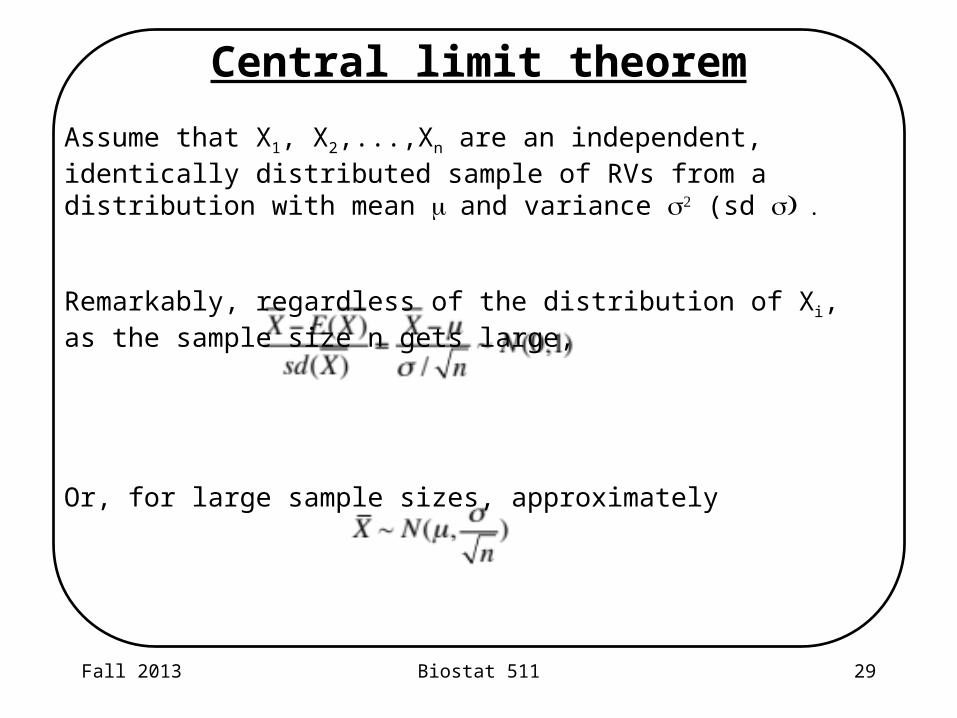
Central limit theorem
Assume that X1, X2,...,Xn are an independent, identically distributed sample of RVs from a distribution with mean m and variance s2 (sd ) .s
Remarkably, regardless of the distribution of Xi, as the sample size n gets large,
Or, for large sample sizes, approximately

Fall 2013 Biostat 511 30
Central limit theorem at work
The CLT is very powerful: no matter how skewed the distribution of X, the distribution of a sample mean will approach normality with increasing n.
How large does n need to be for the normal approximation to be good?
It depends on the distribution of X.
Distribution of sample mean for different N
Fall 2013 Biostat 511 31
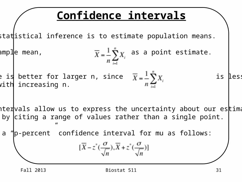
Confidence intervals
One goal of statistical inference is to estimate population means.
We use the sample mean, as a point estimate.
This estimate is better for larger n, since is less variable andcloser to m with increasing n.
Confidence intervals allow us to express the uncertainty about our estimate of the mean, by citing a range of values rather than a single point.
We construct a “p-percent” confidence interval for mu as follows:
Fall 2013 Biostat 511 32
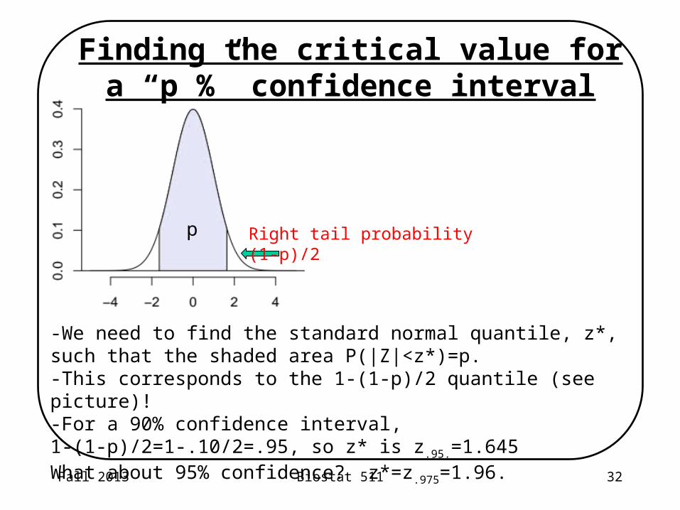
Finding the critical value for a “p %” confidence interval
-We need to find the standard normal quantile, z*, such that the shaded area P(|Z|<z*)=p.-This corresponds to the 1-(1-p)/2 quantile (see picture)!-For a 90% confidence interval, 1-(1-p)/2=1-.10/2=.95, so z* is z.95.=1.645What about 95% confidence? z*=z.975=1.96.
That is, each of the tail regions have area(1-p)/2. So z* corresponds to the1-(1-p)/2 quantile of the standard normal Distribution.
p Right tail probability(1-p)/2
Fall 2013 Biostat 511 33
Confidence intervals: interpretation
For a given sample, the (for example) 95% confidence interval
either contains the population mean m or it doesn’t!!!
So it doesn’t make sense to to say that there is “a 95% probability that this interval contains .”m
Rather, with repeated samples, a 95% confidence interval constructed with this method will contain 95% m of the time.
Fall 2013 Biostat 511 34
Confidence interval ExampleYour goal is to estimate the mean of systolic BP in a population of women 65-75. You collect a sample of 100 women. Suppose you know that the standard deviation for systolic BP in the population is 20. The mean BP in your sample is 125.
Construct and interpret a 95% confidence interval for the population mean BP.For a 95% CI, the critical value z*=1.96
95% Confidence interval: [125-1.96*20/10, 125+1.96*20/10]=[121.08, 128.92].
Interpretation: with repeated samples, 95% of intervals formed with this method would contain the true mean BP.

Fall 2013 Biostat 511 35
Confidence interval: discussion
What affects the width of the confidence interval?
Confidence intervals depend on the CLT and normal approximation for the sample mean’s distribution. For small n, is this still a good approach?
Recommended