HAL Id: halshs-00658495https://halshs.archives-ouvertes.fr/halshs-00658495
Submitted on 10 Jan 2012
HAL is a multi-disciplinary open accessarchive for the deposit and dissemination of sci-entific research documents, whether they are pub-lished or not. The documents may come fromteaching and research institutions in France orabroad, or from public or private research centers.
L’archive ouverte pluridisciplinaire HAL, estdestinée au dépôt et à la diffusion de documentsscientifiques de niveau recherche, publiés ou non,émanant des établissements d’enseignement et derecherche français ou étrangers, des laboratoirespublics ou privés.
Extreme Value at Risk and Expected Shortfall duringFinancial Crisis
L. Kourouma, D. Dupre, G. Sanfilippo, O. Taramasco
To cite this version:L. Kourouma, D. Dupre, G. Sanfilippo, O. Taramasco. Extreme Value at Risk and Expected Shortfallduring Financial Crisis. Cahier de recherche du CERAG 2011-03 E2. 2011. <halshs-00658495>
Extreme Value at Risk and Expected Shortfall during Financial Crisis
Lanciné Kourouma
Denis Dupre
Gilles Sanfilippo
Ollivier Taramasco
CAHIER DE RECHERCHE n°2011-03 E2
Unité Mixte de Recherche CNRS / Université Pierre Mendès France Grenoble 2
150 rue de la Chimie – BP 47 – 38040 GRENOBLE cedex 9
Tél. : 04 76 63 53 81 Fax : 04 76 54 60 68
2
Extreme Value at Risk and Expected Shortfall during
Financial Crisis
Lanciné Kourouma1, Denis Dupre2, Gilles Sanfilippo3, Ollivier Taramasco4 CERAG UMR5820 – Doctoral School of Management
University of Grenoble - France
April 2011
Abstract
This paper investigates Value at Risk and Expected Shortfall for CAC 40, S&P 500,
Wheat and Crude Oil indexes during the 2008 financial crisis. We show an underestimation
of the risk of loss for the unconditional VaR models as compared with the conditional models.
This underestimation is stronger using the historical VaR approach than when using the
extreme values theory VaR model. Even in 2008 financial crisis, the conditional EVT model
is more accurate and reliable for predicting the asset risk losses. Banks have no interest in
using it because the Basel II agreement penalizes banks using accuracy models like the
conditional EVT model, and this is the case for the assets being studied in this paper.
JEL classification: C22; G10; G21
Keywords: Market risk, Value at Risk, EVT, GARCH, Financial crisis, Basel requirements
1 IAE of Grenoble – CERAG UMR CNRS 5820 (CERAG, 150, rue de la chimie, BP 47, 38040 Grenoble cedex). E-mail : [email protected]; 2 IAE of Grenoble – CERAG UMR CNRS 5820 (CERAG, 150, rue de la chimie, BP 47, 38040 Grenoble cedex). E-mail : Denis.Dupré@upmf-grenoble.fr 3 IAE of Grenoble – CERAG UMR CNRS 5820 (CERAG, 150, rue de la chimie, BP 47, 38040 Grenoble cedex). E-mail : [email protected] 4 ENSIMAG of Grenoble – CERAG UMR CNRS 5820 (CERAG, 150, rue de la chimie, BP 47, 38040 Grenoble cedex). E-mail : [email protected]
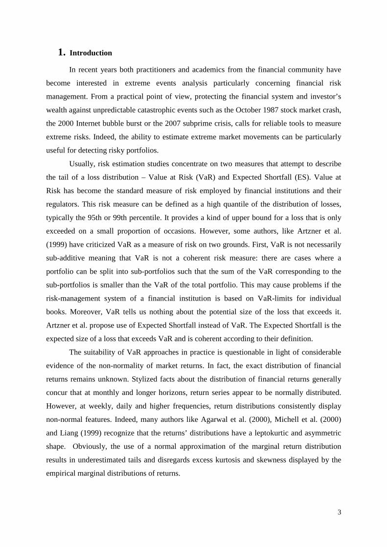
3
1. Introduction
In recent years both practitioners and academics from the financial community have
become interested in extreme events analysis particularly concerning financial risk
management. From a practical point of view, protecting the financial system and investor’s
wealth against unpredictable catastrophic events such as the October 1987 stock market crash,
the 2000 Internet bubble burst or the 2007 subprime crisis, calls for reliable tools to measure
extreme risks. Indeed, the ability to estimate extreme market movements can be particularly
useful for detecting risky portfolios.
Usually, risk estimation studies concentrate on two measures that attempt to describe
the tail of a loss distribution – Value at Risk (VaR) and Expected Shortfall (ES). Value at
Risk has become the standard measure of risk employed by financial institutions and their
regulators. This risk measure can be defined as a high quantile of the distribution of losses,
typically the 95th or 99th percentile. It provides a kind of upper bound for a loss that is only
exceeded on a small proportion of occasions. However, some authors, like Artzner et al.
(1999) have criticized VaR as a measure of risk on two grounds. First, VaR is not necessarily
sub-additive meaning that VaR is not a coherent risk measure: there are cases where a
portfolio can be split into sub-portfolios such that the sum of the VaR corresponding to the
sub-portfolios is smaller than the VaR of the total portfolio. This may cause problems if the
risk-management system of a financial institution is based on VaR-limits for individual
books. Moreover, VaR tells us nothing about the potential size of the loss that exceeds it.
Artzner et al. propose use of Expected Shortfall instead of VaR. The Expected Shortfall is the
expected size of a loss that exceeds VaR and is coherent according to their definition.
The suitability of VaR approaches in practice is questionable in light of considerable
evidence of the non-normality of market returns. In fact, the exact distribution of financial
returns remains unknown. Stylized facts about the distribution of financial returns generally
concur that at monthly and longer horizons, return series appear to be normally distributed.
However, at weekly, daily and higher frequencies, return distributions consistently display
non-normal features. Indeed, many authors like Agarwal et al. (2000), Michell et al. (2000)
and Liang (1999) recognize that the returns’ distributions have a leptokurtic and asymmetric
shape. Obviously, the use of a normal approximation of the marginal return distribution
results in underestimated tails and disregards excess kurtosis and skewness displayed by the
empirical marginal distributions of returns.
4
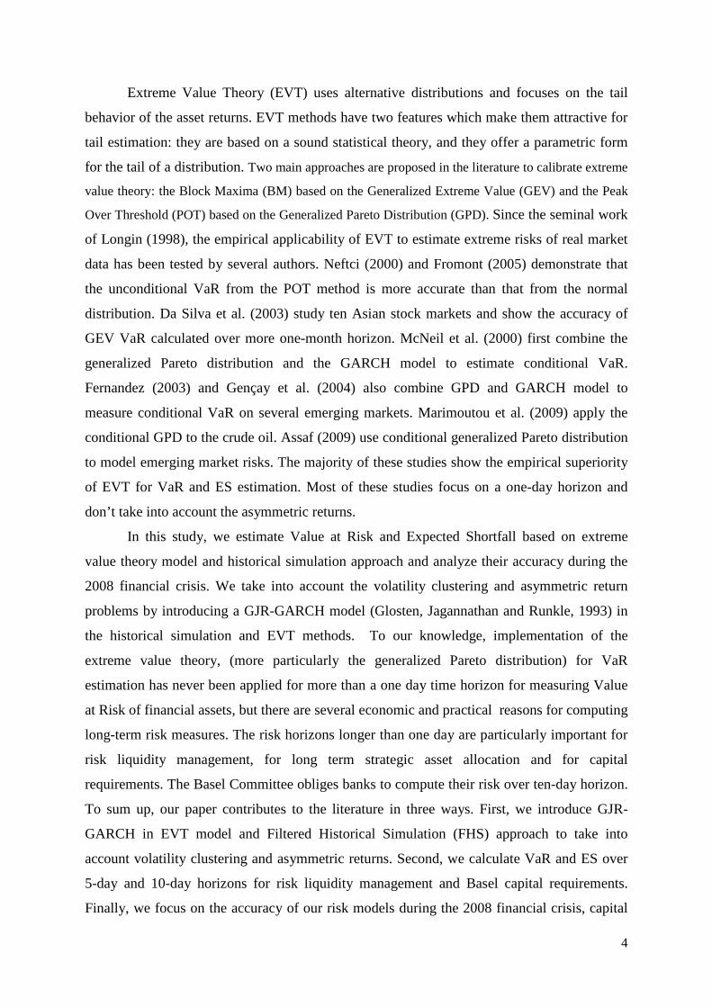
Extreme Value Theory (EVT) uses alternative distributions and focuses on the tail
behavior of the asset returns. EVT methods have two features which make them attractive for
tail estimation: they are based on a sound statistical theory, and they offer a parametric form
for the tail of a distribution. Two main approaches are proposed in the literature to calibrate extreme
value theory: the Block Maxima (BM) based on the Generalized Extreme Value (GEV) and the Peak
Over Threshold (POT) based on the Generalized Pareto Distribution (GPD). Since the seminal work
of Longin (1998), the empirical applicability of EVT to estimate extreme risks of real market
data has been tested by several authors. Neftci (2000) and Fromont (2005) demonstrate that
the unconditional VaR from the POT method is more accurate than that from the normal
distribution. Da Silva et al. (2003) study ten Asian stock markets and show the accuracy of
GEV VaR calculated over more one-month horizon. McNeil et al. (2000) first combine the
generalized Pareto distribution and the GARCH model to estimate conditional VaR.
Fernandez (2003) and Gençay et al. (2004) also combine GPD and GARCH model to
measure conditional VaR on several emerging markets. Marimoutou et al. (2009) apply the
conditional GPD to the crude oil. Assaf (2009) use conditional generalized Pareto distribution
to model emerging market risks. The majority of these studies show the empirical superiority
of EVT for VaR and ES estimation. Most of these studies focus on a one-day horizon and
don’t take into account the asymmetric returns.
In this study, we estimate Value at Risk and Expected Shortfall based on extreme
value theory model and historical simulation approach and analyze their accuracy during the
2008 financial crisis. We take into account the volatility clustering and asymmetric return
problems by introducing a GJR-GARCH model (Glosten, Jagannathan and Runkle, 1993) in
the historical simulation and EVT methods. To our knowledge, implementation of the
extreme value theory, (more particularly the generalized Pareto distribution) for VaR
estimation has never been applied for more than a one day time horizon for measuring Value
at Risk of financial assets, but there are several economic and practical reasons for computing
long-term risk measures. The risk horizons longer than one day are particularly important for
risk liquidity management, for long term strategic asset allocation and for capital
requirements. The Basel Committee obliges banks to compute their risk over ten-day horizon.
To sum up, our paper contributes to the literature in three ways. First, we introduce GJR-
GARCH in EVT model and Filtered Historical Simulation (FHS) approach to take into
account volatility clustering and asymmetric returns. Second, we calculate VaR and ES over
5-day and 10-day horizons for risk liquidity management and Basel capital requirements.
Finally, we focus on the accuracy of our risk models during the 2008 financial crisis, capital
5
requirement measures and the opportunity of banks to choose a reliable model. The remainder
of this paper is organized as follows. In Section 2 we present our data sample and its
descriptive statistics. We present generalized Pareto distribution parameter estimate in section
3. We also check the adequacy between the empirical and theoretical generalized Pareto
distributions. Section 4 explains relevant back-testing procedures for testing the accuracy of
VaR and ES estimates. In section 5, our empirical results from the Historical Simulation
method and EVT model are presented. Finally, Section 6 concludes and gives some
suggestions for future research.
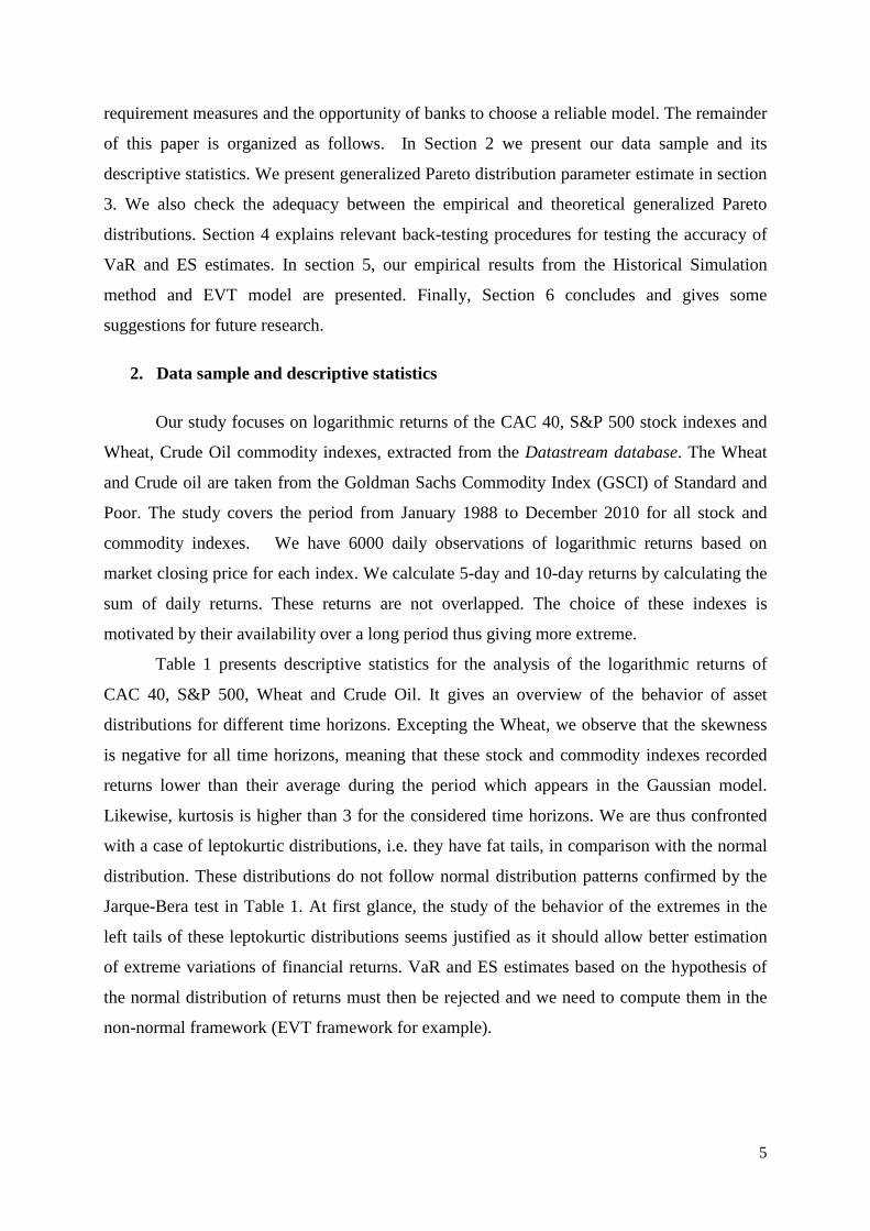
2. Data sample and descriptive statistics
Our study focuses on logarithmic returns of the CAC 40, S&P 500 stock indexes and
Wheat, Crude Oil commodity indexes, extracted from the Datastream database. The Wheat
and Crude oil are taken from the Goldman Sachs Commodity Index (GSCI) of Standard and
Poor. The study covers the period from January 1988 to December 2010 for all stock and
commodity indexes. We have 6000 daily observations of logarithmic returns based on
market closing price for each index. We calculate 5-day and 10-day returns by calculating the
sum of daily returns. These returns are not overlapped. The choice of these indexes is
motivated by their availability over a long period thus giving more extreme.
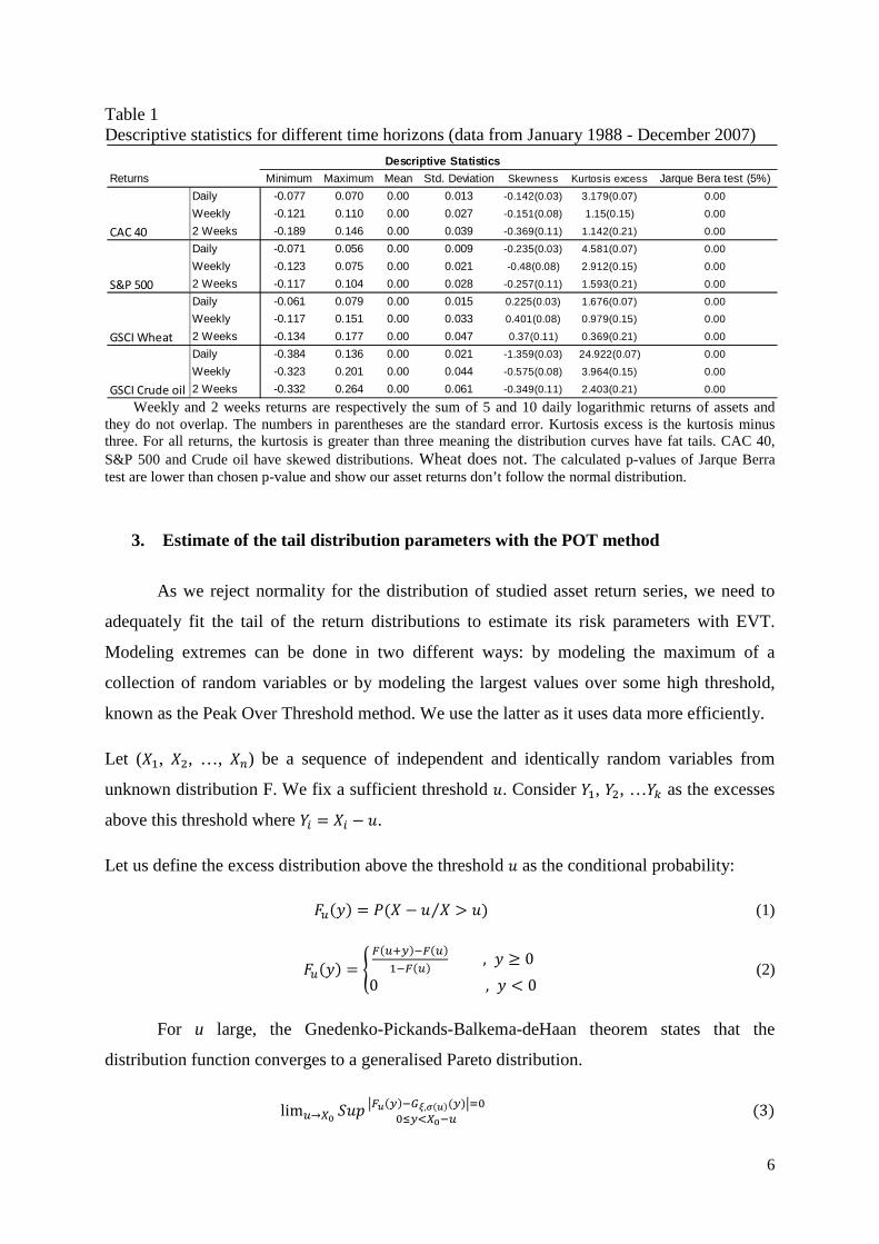
Table 1 presents descriptive statistics for the analysis of the logarithmic returns of
CAC 40, S&P 500, Wheat and Crude Oil. It gives an overview of the behavior of asset
distributions for different time horizons. Excepting the Wheat, we observe that the skewness
is negative for all time horizons, meaning that these stock and commodity indexes recorded
returns lower than their average during the period which appears in the Gaussian model.
Likewise, kurtosis is higher than 3 for the considered time horizons. We are thus confronted
with a case of leptokurtic distributions, i.e. they have fat tails, in comparison with the normal
distribution. These distributions do not follow normal distribution patterns confirmed by the
Jarque-Bera test in Table 1. At first glance, the study of the behavior of the extremes in the
left tails of these leptokurtic distributions seems justified as it should allow better estimation
of extreme variations of financial returns. VaR and ES estimates based on the hypothesis of
the normal distribution of returns must then be rejected and we need to compute them in the
non-normal framework (EVT framework for example).
6
Table 1 Descriptive statistics for different time horizons (data from January 1988 - December 2007)
Weekly and 2 weeks returns are respectively the sum of 5 and 10 daily logarithmic returns of assets and they do not overlap. The numbers in parentheses are the standard error. Kurtosis excess is the kurtosis minus three. For all returns, the kurtosis is greater than three meaning the distribution curves have fat tails. CAC 40, S&P 500 and Crude oil have skewed distributions. Wheat does not. The calculated p-values of Jarque Berra test are lower than chosen p-value and show our asset returns don’t follow the normal distribution.
3. Estimate of the tail distribution parameters with the POT method
As we reject normality for the distribution of studied asset return series, we need to
adequately fit the tail of the return distributions to estimate its risk parameters with EVT.
Modeling extremes can be done in two different ways: by modeling the maximum of a
collection of random variables or by modeling the largest values over some high threshold,
known as the Peak Over Threshold method. We use the latter as it uses data more efficiently.
Let (��, ��, …, ��) be a sequence of independent and identically random variables from
unknown distribution F. We fix a sufficient threshold �. Consider ��, ��, …�� as the excesses
above this threshold where �� �� �.
Let us define the excess distribution above the threshold � as the conditional probability:
�� �� � � � � � �� ⁄ (1)
�� �� � � ������ ����� �� , � � 00 , � � 0� (2)
For u large, the Gnedenko-Pickands-Balkema-deHaan theorem states that the
distribution function converges to a generalised Pareto distribution.
lim�!"# $�% &�' ���(),* '� ��&+,,-�."#�� 3�
Minimum Maximum Mean Std. Deviation Skewness Kurtosis excess Jarque Bera test (5%)
Daily -0.077 0.070 0.00 0.013 -0.142(0.03) 3.179(0.07) 0.00
Weekly -0.121 0.110 0.00 0.027 -0.151(0.08) 1.15(0.15) 0.00
2 Weeks -0.189 0.146 0.00 0.039 -0.369(0.11) 1.142(0.21) 0.00
Daily -0.071 0.056 0.00 0.009 -0.235(0.03) 4.581(0.07) 0.00
Weekly -0.123 0.075 0.00 0.021 -0.48(0.08) 2.912(0.15) 0.00
2 Weeks -0.117 0.104 0.00 0.028 -0.257(0.11) 1.593(0.21) 0.00
Daily -0.061 0.079 0.00 0.015 0.225(0.03) 1.676(0.07) 0.00
Weekly -0.117 0.151 0.00 0.033 0.401(0.08) 0.979(0.15) 0.00
2 Weeks -0.134 0.177 0.00 0.047 0.37(0.11) 0.369(0.21) 0.00
Daily -0.384 0.136 0.00 0.021 -1.359(0.03) 24.922(0.07) 0.00
Weekly -0.323 0.201 0.00 0.044 -0.575(0.08) 3.964(0.15) 0.00
2 Weeks -0.332 0.264 0.00 0.061 -0.349(0.11) 2.403(0.21) 0.00
S&P 500
GSCI Wheat
GSCI Crude oil
Descriptive Statistics
Returns
CAC 40
7
where 01,2 is the generalized Pareto distribution and given by:
01,2 �� 31 1 5 1�2 ��� 16 , 7 8 01 exp< � =6 > , 7 0� (4)
where � � 0 for ξ � 0 and 0 @ � @ =/ξ for ξ � 0.
The parameter ξ determines the shape of the distribution, and in particular the decay of the
left tail or heavy tailed behaviour. The parameter σ is a scale parameter and the location
parameter u will be the threshold value. The generalized Pareto distribution subsumes three
other distributions under its parameterization. So, when shape parameter 7 0, we obtain a
type 1 distribution (tails decrease exponentially) like the normal distribution. If 7 � 0, we
have a type 2 distribution (tails are finite) like a beta distribution. For 7 � 0, we obtain a type
3 distribution (tails decrease polynomially) as student’s t distribution. Assuming a GPD
function for the tail distribution, analytical expressions for VaR and ES can be defined as a
function of GPD parameters.
BCDEF � 5 2G1H IJ KK' 1 ��L�1H 1M (6)
N is the number of observations in the left tail and N� is the number of excesses beyond the threshold �.
The Expected Shortfall based on the GPD approach is defined as:
O$EF BCDEF 5 P�Q RSTUG�����Q RSTUG��Q 5 P�Q���Q (7)
3.1. Conditional Generalized Pareto Distribution modelling
To take into account the volatility clustering in our studied assets we combine the POT
method and GARCH model as first suggested by McNeil and Frey (2000). GJR-GARCH type
(Glosten, Jagannathan and Runkle, 1993) is used to model the conditional VaR. The
advantage of this GARCH-EVT combination lies in its ability to capture conditional
heteroscedascity in the data through the GARCH framework, while at the same time modeling
the extreme tail behavior through the EVT method. GARCH models explicitly model the
conditional volatility as a function of past conditional volatilities and returns. We assume that
the dynamics of the return series follows the stochastic process of GJR-GARCH(1,1):
8
�V WV 5 XV Y, 5 Y��V�� 5 ZV=[,V (8)
WV Y, 5 Y��V�� (9)
=[,V� \, 5 \�XV��� 5 ] _`ab.,XV��� 5 \�=[,V��� (10)
where _`ab 0 if XV�� � 0 and _`ab 1 otherwise, that allows to take into account the sign
of the residuals’ disturbance. WV represents the conditional mean, XV the residuals, ZV the
standardized residuals, =[,V� the variance and Y�, \� are the parameters of the estimation.
The combined approach, denoted as conditional GPD, has the following steps:
• Step 1: Fit a GJR-GARCH model to the return data by quasi-maximum likelihood.
That is, maximize the log-likelihood function of the sample assuming normal
innovations. Estimate WV and =[,V from the fitted model and extract the standardized
residuals ZV. • Step 2: Consider the standardized residuals computed in step 1 to be realizations of a
white noise process, and estimate the tails of the innovations using extreme value
theory. Next, compute the quantiles of the innovations.
• Step 3: Construct VaR from parameters estimated in steps one and two. VaR is
computing with le same formula in Eq. (6). The conditional Expected Shortfall is
given by:
O$EF u 5 σe fBCDEF1 ξ 5 σ ξ�1 ξ g 11�
where σe is forecasted volatility from GJR-GARCH modeling.
By first filtering the returns with a GJR-GARCH model, we essentially get i.i.d. series on
which it is straightforward to apply the EVT technique. The main advantage of the
conditional generalized Pareto distribution is that it produces a VaR which reflects the current
volatility background.
3.2.Threshold choice for EVT
To apply the GPD, we need to choose a reasonable threshold �, which determines the
number of observations, N�, in excess of threshold value. The choice of the threshold � is an
important issue: on one hand, if � is too high, it results in too few excesses and consequently
9
high variance estimators and on the other hand, if � too small, it provides biased estimators
and the approximation to a GPD is not feasible. It is possible to choose an asymptotically
optimal threshold by a quantification of a bias versus variance trade-off. So far, no automatic
algorithm with satisfactory performance for the selection of the threshold u is available. For
example, Gavin (2000) and Neftci (2000) arbitrarily chose to retain respectively 10 % and 5
% of the sample while McNeil and Frey (2000) use the mean excess plot. (ME plot), defined
in the following way:
h u, ei u��, Xi:i � � � X�:il (12)
m� �� �K� ∑ K��+� �o ��� (13)
where X�:i et Xi:i are respectively the maximums and the minimums of the sample and
m� ��, the sum of the excesses over the threshold � divided by the number N� of data which
exceed �. It is necessary to note that the mean excess function (ME) of the generalized Pareto
distribution is:
m� �� 2�1���1 , ξ � 1 (14)
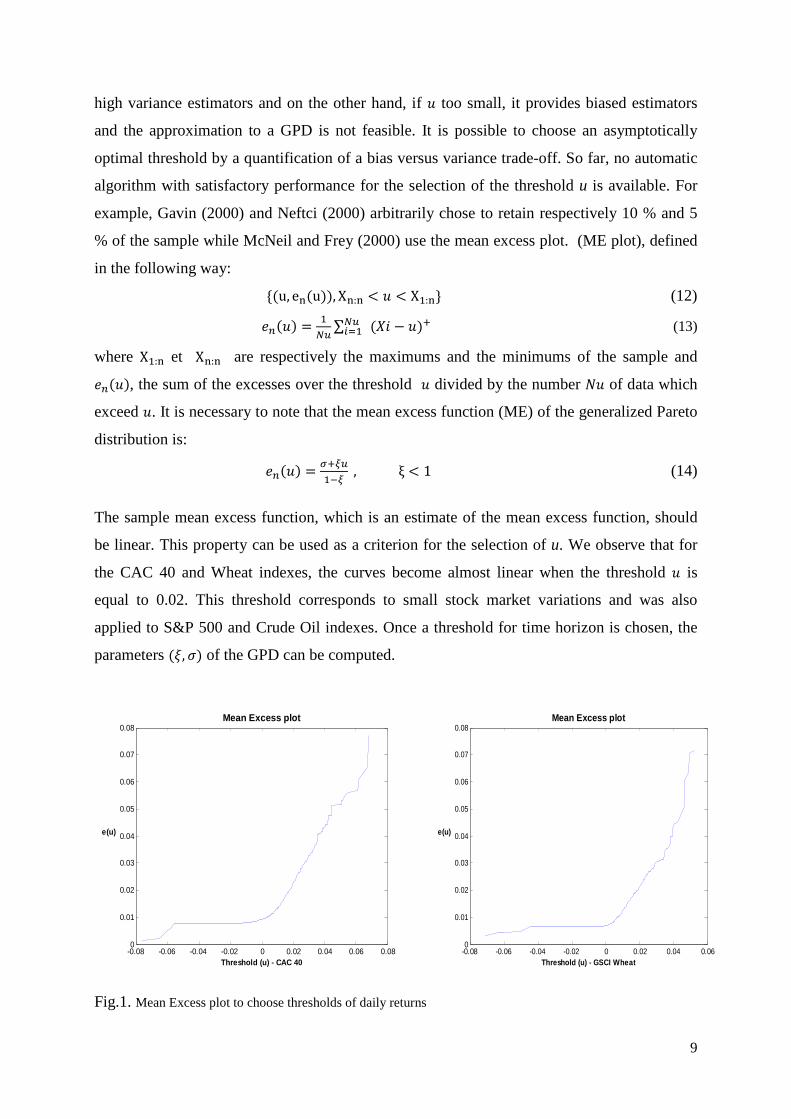
The sample mean excess function, which is an estimate of the mean excess function, should
be linear. This property can be used as a criterion for the selection of u. We observe that for
the CAC 40 and Wheat indexes, the curves become almost linear when the threshold � is
equal to 0.02. This threshold corresponds to small stock market variations and was also
applied to S&P 500 and Crude Oil indexes. Once a threshold for time horizon is chosen, the
parameters 7, =� of the GPD can be computed.
Fig.1. Mean Excess plot to choose thresholds of daily returns
-0.08 -0.06 -0.04 -0.02 0 0.02 0.04 0.060
0.01
0.02
0.03
0.04
0.05
0.06
0.07
0.08
Threshold (u) - GSCI Wheat
e(u)
Mean Excess plot
-0.08 -0.06 -0.04 -0.02 0 0.02 0.04 0.06 0.080
0.01
0.02
0.03
0.04
0.05
0.06
0.07
0.08
Threshold (u) - CAC 40
e(u)
Mean Excess plot
10
Different methods can be used to estimate the parameters of the GPD. In this paper we
use the maximum likelihood estimation method. For a sample y = {y1, ..., yn} the log-
likelihood function L(ξ, σ | y) for the GPD is the logarithm of the joint density of the n
observations :
(15)
We compute the values ξ and σ that maximize the log-likelihood function for the sample
defined by the observations exceeding the threshold u.
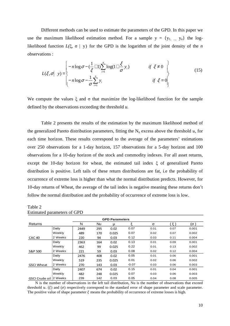
Table 2 presents the results of the estimation by the maximum likelihood method of
the generalized Pareto distribution parameters, fitting the Nu excess above the threshold �, for
each time horizon. These results correspond to the average of the parameters’ estimations
over 250 observations for a 1-day horizon, 157 observations for a 5-day horizon and 100
observations for a 10-day horizon of the stock and commodity indexes. For all asset returns,
except the 10-day horizon for wheat, the estimated tail index ξ of generalized Pareto
distribution is positive. Left tails of these return distributions are fat, i.e the probability of
occurrence of extreme loss is higher than what the normal distribution predicts. However, for
10-day returns of Wheat, the average of the tail index is negative meaning these returns don’t
follow the normal distribution and the probability of occurrence of extreme loss is low.
Table 2 Estimated parameters of GPD
N is the number of observations in the left tail distribution, Nu is the number of observations that exceed threshold �. (7) and (=) respectively correspond to the standard error of shape parameter and scale parameter. The positive value of shape parameter 7 means the probability of occurrence of extreme losses is high.
N Nu µ ξ σ ( ξ ) (σ )Daily 2449 295 0.02 0.07 0.01 0.07 0.001
Weekly 489 170 0.025 0.07 0.02 0.07 0.002
2 Weeks 220 94 0.03 0.12 0.03 0.11 0.004
Daily 2363 164 0.02 0.13 0.01 0.09 0.001
Weekly 462 99 0.025 0.22 0.01 0.13 0.002
2 Weeks 221 59 0.03 0.08 0.02 0.12 0.004
Daily 2476 408 0.02 0.05 0.01 0.06 0.001
Weekly 519 235 0.025 0.01 0.02 0.06 0.002
2 Weeks 270 143 0.03 -0.07 0.03 0.06 0.003
Daily 2407 674 0.02 0.15 0.01 0.04 0.001
Weekly 482 248 0.025 0.07 0.03 0.06 0.003
2 Weeks 239 142 0.03 0.05 0.04 0.08 0.005
S&P 500
GSCI Wheat
GSCI Crude oil
Returns
CAC 40
GPD Parameters
=−−
≠++−−=
∑
∑
=
=
01
log
0)1log()11
(log
),(
1
1
ξσ
σ
ξσξ
ξσ
σξifyn
ifyn
yLn
ii
n
ii
11
To validate the previous results, we have to test the adequacy of the estimated asymptotic
distributions to represent the behavior of the extreme returns of the considered assets. For that
purpose, we use a graphical tool and a statistical test.
3.3. Goodness of fit test
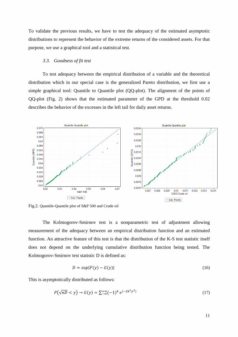
To test adequacy between the empirical distribution of a variable and the theoretical
distribution which in our special case is the generalized Pareto distribution, we first use a
simple graphical tool: Quantile to Quantile plot (QQ-plot). The alignment of the points of
QQ-plot (Fig. 2) shows that the estimated parameter of the GPD at the threshold 0.02
describes the behavior of the excesses in the left tail for daily asset returns.
Fig.2. Quantile-Quantile plot of S&P 500 and Crude oil
The Kolmogorov-Smirnov test is a nonparametric test of adjustment allowing
measurement of the adequacy between an empirical distribution function and an estimated
function. An attractive feature of this test is that the distribution of the K-S test statistic itself
does not depend on the underlying cumulative distribution function being tested. The
Kolmogorov-Smirnov test statistic D is defined as:
p q�%|� �� 0 ��| (16)
This is asymptotically distributed as follows:
�<√tp � �> ! 0 �� ∑ 1���u�u m ���v�v� (17)
12
Where � �� and 0 �� represent the empirical distribution function and estimated function of
the generalized Pareto distribution. The hypothesis regarding the distributional form is
rejected if the test statistic D is greater than the critical value.
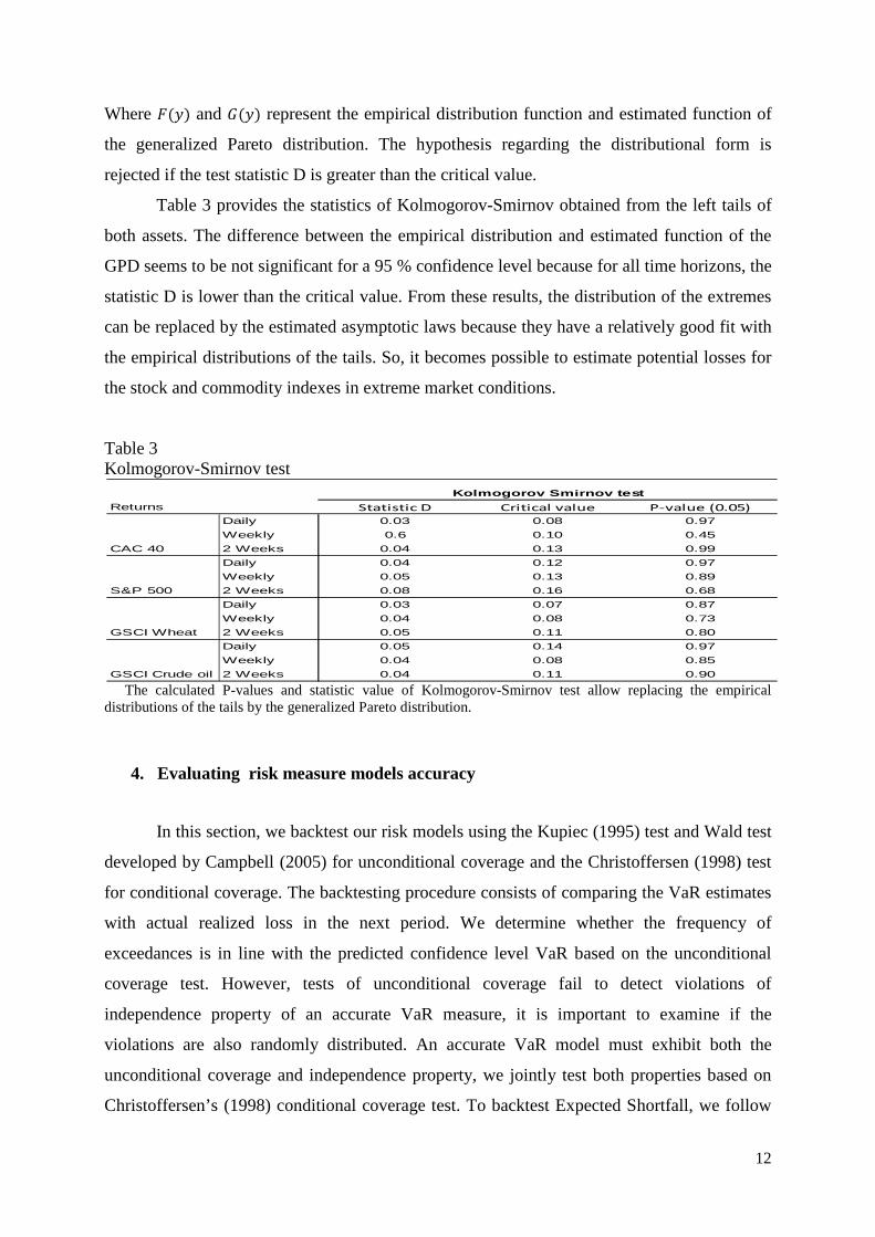
Table 3 provides the statistics of Kolmogorov-Smirnov obtained from the left tails of
both assets. The difference between the empirical distribution and estimated function of the
GPD seems to be not significant for a 95 % confidence level because for all time horizons, the
statistic D is lower than the critical value. From these results, the distribution of the extremes
can be replaced by the estimated asymptotic laws because they have a relatively good fit with
the empirical distributions of the tails. So, it becomes possible to estimate potential losses for
the stock and commodity indexes in extreme market conditions.
Table 3 Kolmogorov-Smirnov test
The calculated P-values and statistic value of Kolmogorov-Smirnov test allow replacing the empirical distributions of the tails by the generalized Pareto distribution.
4. Evaluating risk measure models accuracy
In this section, we backtest our risk models using the Kupiec (1995) test and Wald test
developed by Campbell (2005) for unconditional coverage and the Christoffersen (1998) test
for conditional coverage. The backtesting procedure consists of comparing the VaR estimates
with actual realized loss in the next period. We determine whether the frequency of
exceedances is in line with the predicted confidence level VaR based on the unconditional
coverage test. However, tests of unconditional coverage fail to detect violations of
independence property of an accurate VaR measure, it is important to examine if the
violations are also randomly distributed. An accurate VaR model must exhibit both the
unconditional coverage and independence property, we jointly test both properties based on
Christoffersen’s (1998) conditional coverage test. To backtest Expected Shortfall, we follow
Returns Statistic D Critical value P-value (0.05)
Daily 0.03 0.08 0.97
Weekly 0.6 0.10 0.45
2 Weeks 0.04 0.13 0.99
Daily 0.04 0.12 0.97
Weekly 0.05 0.13 0.89
2 Weeks 0.08 0.16 0.68
Daily 0.03 0.07 0.87
Weekly 0.04 0.08 0.73
2 Weeks 0.05 0.11 0.80
Daily 0.05 0.14 0.97
Weekly 0.04 0.08 0.85
2 Weeks 0.04 0.11 0.90
CAC 40
S&P 500
GSCI Wheat
GSCI Crude oil
Kolmogorov Smirnov test
13
the backtesting procedure used by Embrechts et al. (2005) in calculating a measure evaluating
ES performance when returns are violating the corresponding VaR measure.
4.1. Unconditional coverage test
Let N ∑ V��wV+� be the number of days over a T period that the portfolio loss was larger than the VaR estimate, where V�� is a sequence of VaR violations that can be described as:
V�� x1, oy �V�� � BCDV��/z0, oy �V�� � BCDV��/z{ (18)
We use a likelihood ratio test developed by Kupiec (1995). This test examines whether the failure rate Y is statistically equal to the expected one. If the total number of such trials is T, the number of failure N can be modeled with a binomial distribution with probability of
occurrence equaling Y. The correct null and alternative hypothesis are, respectively |, : Kw Y and |� : Kw 8 Y.
The appropriate likelihood ratio statistic is:
}D�~ 2 �log fJKwLK J1 KwLw�Kg log YK 1 Y�w�K�� , }D�~ �! �� 1� (19)
}D�~ �! �� 1� under |, of good specification. Note that this backtesting procedure is a two-sided test. Therefore, a model is rejected if it generates too many or too few violations, but based on it, the risk manager can accept a model that generates dependent exceptions.
The Kupiec test doesn’t indicate if the risk model underestimates or overestimates the risk losses. To remedy that, we apply the Wald test which is defined by its statistic z:
Z √� YG Y��Y 1 Y� , � �! N 0,1� 20�
Where YG is the risk level estimated by the model, Y is the chosen risk level and T the size of
retained backtesting window.
The hypothesis of unconditional coverage is rejected when statistic z is different from 0 or
higher than the critical value of normal distribution associated with a certain confidence level.
If the statistic is raised and negative, it means that the considered model significantly
overestimates the risk of the asset while a positive value indicates an underestimation of the
risk. Statistic z equal to zero indicates that the real number of VaR violations is identical at
the risk level fixed for the calculation of the VaR. In this last scenario, it is considered that the
model reliably allows in estimating asset risk.
14
4.2.Conditional coverage test
The unconditional coverage test may fail to detect VaR measures that exhibit correct
unconditional coverage but exhibit dependent VaR violations. So, we turn to a Christoffersen
test, which jointly investigates if the VaR failure process is independently distributed through
time. This test provides an opportunity to detect VaR measures which are deficient in one way
or another. Under the null hypothesis that the failure process is independent and the expected
proportion of violations is equal to Y, the appropriate likelihood ratio is:
}D~~ 2�log YK 1 Y�w�K�� (21)
52�log 1 �,���##�,��#b� 1 �����b#����bb� , }�� �! �� 2�
Where t�� is the number of observations with value o followed by �, for o, � 0,1 and ��� ���∑ ���� are the corresponding probabilities. The values o, � 1 denote that a violation has
been made, while o, � 0 indicates the opposite. The main advantage of this test is that it can reject a VaR model that generates either too many or too few clustered violations.
4.3. Expected Shortfall backtesting
To backtest the ES forecasts, we calculate the average difference between the realized returns and the forecasted ES’s, conditional on having a (negative) returns exceeding the corresponding VaR estimate.
The test statistic is defined as follows:
B ∑ �V O$V,��� "`.RST`,��V+� ∑ "`.RST`,��V+� 22�
Given this formula, the negative value of the statistic indicates the underestimation of risk
losses and the positive value, the risk losses’ overestimation. ES measures are accurate when
the value of the B tends to zero.
We choose to test the risk models over 250 days for a 1-day horizon, over 157 weeks
for a 5-day horizon and over 100 2-weeks for a 10-day horizon. This time window of 250
working days was recommended by the Basel committee as a backtesting window for the
validation of internal models of market risk measure. Besides, in the document "Risk
Management: In practical Guides" of the RiskMetrics group, this window is fixed at 90 days
15
minimum to obtain significant results. These periods includes the time of the Lehman
Brothers5 bankruptcy corresponding to the bottom of the 2008 financial crisis.
5. Empirical results
Our empirical analysis differs from previous empirical research in two respects. First,
most previous research has analyzed only VaR at the 95% and 99% confidence levels. To
better reflect the extreme market conditions of this research we consider confidence levels for
VaR and ES of 95%, 99% and 99.5%. The accuracy of our measures is assessed using 5,216
observations for a 1-day horizon, 1,042 observations for a 5-day horizon and 499 observations
for a 10-day horizon. Second, to take into account for market liquidity constraints and Basel
regulations we consider a 5-day and 10-day risk horizons in addition to the more typical 1-day
horizon. That allows calculating VaR over 10-day horizon without multiplying by the square
root of 10. This rule is problematic for VaR measurement using the EVT model. According to
the extreme value theory, to compute VaR over a time horizon, the daily VaR must be
multiplied by the time horizon exponent of the tail index value of the generalized Pareto
distribution which is less than 0.5 for financial assets. Following this rule, the VaR measures
of the EVT model will underestimate financial risks. Each time VaR and ES are estimated,
they are based on revised parameter estimates using the most recent estimation window of
5,216 days, 1,042 weeks and 499 10-days for different time horizon. At the end of each risk
horizon we calculate actual profit and loss for the trading portfolio. An exceedance occurs if
the loss is greater than the estimated VaR or ES for that horizon. These exceedances are
imputs to the tests of unconditional coverage, conditional coverage and ES backtest. Tables 4
and 5 present results for the unconditional and conditional Historical Simulation and EVT
methods.
Clearly the unconditional HS method performs no better in tests of unconditional
coverage (column (i.d) and column (i.e)) and of conditional coverage (column (i.f)). The
performance in measuring ES (column (i.g)) is poor for different time horizons. The Wald test
on the unconditional HS method indicates a strong underestimation for stock and commodity
indexes over 1-day horizon. These underestimations decrease when the time horizon
increases.
5 Lehman Brothers was an Investment bank in the USA which went bankrupt on September 15th, 2008 during the 2008 financial crisis.
16
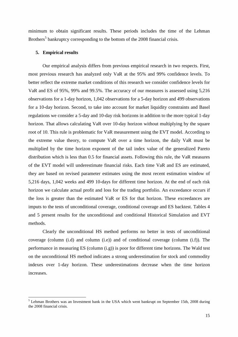
Table 4 Unconditional risk models backtesting
(a) The trading portfolio used for the analysis. (b) The confidence level at which VaR and ES are calculated. (c) The number of times that VaR is exceeded by real losses. (d) and (e) Test of null hypothesis that the actual number of violations is equal to the expected number of violations. (f) Joint test of the null hypothesis that violations spread evenly over time. (g) Test the underestimation or the overestimation of losses beyond the VaR. The back-testing runs from January, 2008 to December, 2008 for the 1-day horizon, from January, 2008 to December, 2010 for the 5-day horizon and from Mars, 2007 to December, 2010 for the 10-day horizon. The values in the parentheses correspond at the p-value which must compare to Y for columns (c) and (d) concerning respectively VaR violations and the Wald test. For Kupiec and Christoffersen tests, p-value has to compare to 5%.
Considering the unconditional EVT model, its backtesting results in Table 4 shows a
slight underestimation of risk losses for our stock and commodity indexes at a 1-day horizon.
However, according to Wald, Kupiec and Christoffersen tests, the unconditional EVT model
performs better over 5-day and 10-day horizons. The Expected Shortfall based on the EVT
model is poor but less than that of the Historical Simulation method. That is, the ES (ES6 test
statistic in column (i.g) and (ii.g) of Table 4) underestimate the true potential losses beyond
the VaR. The unconditional EVT model performs better in backtesting test than the
unconditional Historical Simulation method. The EVT model has advantages to be modeled
on the extreme left tail of asset returns. However, both models underestimate risk losses at a
1-day horizon. This underestimation can be explained in part by the presence of the clustering
volatility. To take into account this clustering volatility, we introduce in our risk models the
GJR-GARCH modeling to compute the conditional VaR and ES’ measures. Moreover, this
6 The negative values of ES test statistic indicate the real losses are superior to the expected shortfall value. Embrechts et al. (2005) take the absolute of this statistic to appreciate the model accuracy. Don’t take the absolute value make sense to know about model underestimation or model overestimation.
Assets 1-α (i) Unconditional HS (ii) Unconditional EVT(a) (b)
VaR violations
Wald test
statistic
Kupiec test
statistic
Christoffersen
test statistic
ES test
statistic VaR violations
Wald test
statistic
Kupiec test
statistic
Christoffersen
test statistic
ES test
statistic
( c ) (d) ( e ) ( f ) ( g ) ( c ) (d) ( e ) ( f ) ( g )
1 -day horizon
CAC 40 95.00 40(0.00) 7.98(0.00) 41.37(0.00) 41.37(0.00) -0.0098 26(0.00) 3.92(0.00) 11.87(0.00) 11.87(0.00) -0.0104
99.00 19(0.00) 9.22(0.00) 37.04(0.00) 37.04(0.00) -0.0089 13(0.00) 6.67(0.00) 22.32(0.00) 22.32(0.00) -0.0052
99.50 13(0.00) 10.54(0.00) 37.95(0.00) 37.95(0.00) -0.0062 9(0.00) 6.95(0.00) 20.28(0.00) 20.78(0.00) -0.0024
S&P 500 95.00 50(0.00) 10.88(0.00) 69.89(0.00) 69.89(0.00) -0.0131 39(0.00) 7.69(0.00) 38.82(0.00) 38.82(0.00) -0.0113
99.00 27(0.00) 15.57(0.00) 82.01(0.00) 82.01(0.00) -0.0115 18(0.00) 9.85(0.00) 41.06(0.00) 41.27(0.00) -0.0105
99.50 21(0.00) 17.71(0.00) 80.61(0.00) 80.61(0.00) -0.0082 13(0.00) 10.54(0.00) 37.95(0.00) 38.98(0.00) -0.0074
GSCI Wheat 95.00 60(0.00) 13.78(0.00) 103.44(0.00) 103.44(0.00) -0.0109 43(0.00) 8.85(0.00) 49.35(0.00) 49.35(0.00) -0.0106
99.00 33(0.00) 19.39(0.00) 113.22(0.00) 113.22(0.00) -0.0068 25(0.00) 14.30(0.00) 72.24(0.00) 72.24(0.00) -0.0040
99.50 24(0.00) 20.40(0.00) 98.48(0.00) 98.48(0.00) -0.0052 18(0.00) 15.02(0.00) 63.67(0.00) 63.67(0.00) -0.0015
GSCI Crude Oil 95.00 36(0.00) 6.82(0.00) 31.57(0.00) 31.57(0.00) -0.0078 25(0.00) 3.63(0.00) 10.33(0.00) 12.30(0.00) -0.0023
99.00 17(0.00) 9.22(0.00) 37.04(0.00) 37.04(0.00) 0.0097 6(0.01) 2.22(0.01) 3.56(0.06) 3.56(0.17) 0.0051
99.50 7(0.00) 5.16(0.00) 12.75(0.00) 14.32(0.00) 0.0154 4(0.01) 2.47(0.01) 3.84(0.05) 3.84(0.15) 0.0150
5 -day horizon
CAC 40 99.00 6(0.00) 3.55(0.00) 7.36(0.01) 7.37(0.03) -0.0249 3(0.07) 1.15(0.13) 1.04(0.31) 1.04(0.59) -0.0566
S&P 500 99.00 7(0.00) 4.36(0.00) 10.26(0.00) 10.91(0.00) -0.0058 3(0.07) 1.15(0.13) 1.04(0.31) 5.52(0.63) -0.0227
GSCI Wheat 99.00 12(0.00) 8.37(0.00) 28.67(0.00) 28.67(0.00) -0.0086 7(0.00) 4.35(0.00) 10.26(0.00) 10.91(0.00) -0.0150
GSCI Crude Oil 99.00 5(0.01) 2.75(0.00) 4.80(0.03) 6.91(0.03) -0.0031 2(0.21) 0.35(0.37) 0.11(0.74) 0.11(0.95) -0.0360
10 -day horizon
CAC 40 99.00 3(0.02) 2.01(0.02) 2.63(0.11) 2.63(0.27) -0.0495 2(0.08) 1.01(0.16) 0.78(0.38) 0.78(0.68) -0.0547
S&P 500 99.00 4(0.00) 3.02(0.00) 5.18(0.02) 5.19(0.08) -0.0362 2(0.08) 1.01(0.16) 0.78(0.38) 0.78(0.68) -0.0957
GSCI Wheat 99.00 4(0.00) 3.01(0.00) 5.18(0.02) 5.19(0.08) -0.0385 2(0.08) 1.01(0.16) 0.78(0.38) 0.78(0.68) -0.0809
GSCI Crude Oil 99.00 3(0.02) 2.01(0.02) 2.63(0.11) 6.22(0.27) -0.0046 1(0.26) 0.00(0.50) 0.00(1.00) 0.00(0.99) -0.0749
17
GARCH type takes into account the sign of residuals disturbance which has an impact on the
volatility. After taking into account volatility and asymmetric problems in our risk models, we
backtest them in the same way as the previous unconditional risk models.
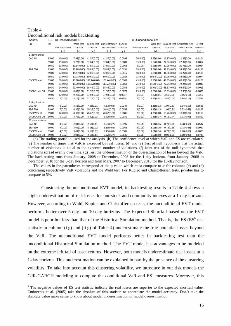
Turning to the conditional Historical Simulation (or Filtered Historical Simulation -
FHS) method presented in Table 5, we observe that while modeling heteroscedasticity
improves performance, especially in terms of unconditional coverage (columns (i.d) and (i.e))
and conditional coverage (column (i.f)). There are slight underestimate according to the
positive values of the Wald test. The Filtered Historical Simulation method performance is
rejected by the backtesting procedure on the Wheat index at a 1-day horizon. The ES statistic
(column (i.g) in Table 5) show that the conditional ES slightly underestimates risk losses.
However, it performs better than its unconditional estimate at a 1-day horizon.
Table 5 Conditional risk models backtesting
(a) The trading portfolio used for the analysis. (b) The confidence level at which VaR and ES are calculated. (c) The number of times that VaR is exceeded by real losses. (d) and (e) Test of null hypothesis that the actual number of violations is equal to the expected number of violations. (f) Joint test of the null hypothesis that violations spread evenly over time. (g) Test the underestimation or the overestimation of losses beyond the VaR. The back-testing runs from January, 2008 to December, 2008 for the 1-day horizon, from January, 2008 to December, 2010 for the 5-day horizon and from Mars, 2007 to December, 2010 for the 10-day horizon. The values in the parentheses correspond at the p-value which must compare to Y for columns (c) and (d) concerning respectively VaR violations and the Wald test. For Kupiec and Christoffersen tests, p-value has to compare to 5%.
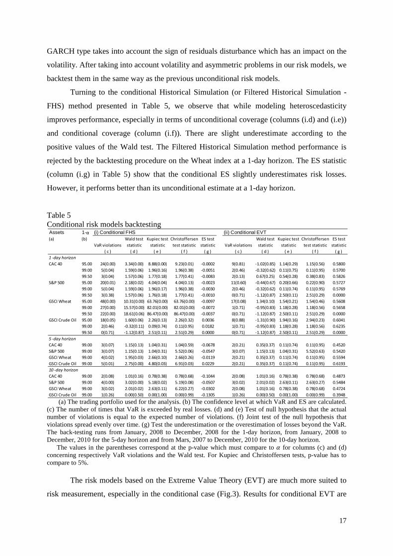
The risk models based on the Extreme Value Theory (EVT) are much more suited to
risk measurement, especially in the conditional case (Fig.3). Results for conditional EVT are
Assets 1-α (i) Conditional FHS (ii) Conditional EVT(a) (b)
VaR violations
Wald test
statistic
Kupiec test
statistic
Christoffersen
test statistic
ES test
statistic VaR violations
Wald test
statistic
Kupiec test
statistic
Christoffersen
test statistic
ES test
statistic
( c ) ( d ) ( e ) ( f ) ( g ) ( c ) ( d ) ( e ) ( f ) ( g )
1 -day horizon
CAC 40 95.00 24(0.00) 3.34(0.00) 8.88(0.00) 9.23(0.01) -0.0002 9(0.81) -1.02(0.85) 1.14(0.29) 1.15(0.56) 0.5800
99.00 5(0.04) 1.59(0.06) 1.96(0.16) 1.96(0.38) -0.0051 2(0.46) -0.32(0.62) 0.11(0.75) 0.11(0.95) 0.5700
99.50 3(0.04) 1.57(0.06) 1.77(0.18) 1.77(0.41) -0.0083 2(0.13) 0.67(0.25) 0.54(0.28) 0.38(0.83) 0.5826
S&P 500 95.00 20(0.01) 2.18(0.02) 4.04(0.04) 4.04(0.13) -0.0023 11(0.60) -0.44(0.67) 0.20(0.66) 0.22(0.90) 0.5727
99.00 5(0.04) 1.59(0.06) 1.96(0.17) 1.96(0.38) -0.0030 2(0.46) -0.32(0.62) 0.11(0.74) 0.11(0.95) 0.5769
99.50 3(0.38) 1.57(0.06) 1.76(0.18) 1.77(0.41) -0.0010 0(0.71) -1.12(0.87) 2.50(0.11) 2.51(0.29) 0.0000
GSCI Wheat 95.00 48(0.00) 10.31(0.00) 63.76(0.00) 63.76(0.00) -0.0097 17(0.08) 1.34(0.10) 1.54(0.21) 1.54(0.46) 0.5608
99.00 27(0.00) 15.57(0.00) 82.01(0.00) 82.01(0.00) -0.0072 1(0.71) -0.95(0.83) 1.18(0.28) 1.18(0.56) 0.5658
99.50 22(0.00) 18.61(0.06) 86.47(0.00) 86.47(0.00) -0.0037 0(0.71) -1.12(0.87) 2.50(0.11) 2.51(0.29) 0.0000
GSCI Crude Oil 95.00 18(0.05) 1.60(0.06) 2.26(0.13) 2.26(0.32) 0.0036 8(0.88) -1.31(0.90) 1.94(0.16) 2.94(0.23) 0.6041
99.00 2(0.46) -0.32(0.11) 0.09(0.74) 0.11(0.95) 0.0182 1(0.71) -0.95(0.83) 1.18(0.28) 1.18(0.56) 0.6235
99.50 0(0.71) -1.12(0.87) 2.51(0.11) 2.51(0.29) 0.0000 0(0.71) -1.12(0.87) 2.50(0.11) 2.51(0.29) 0.0000
5 -day horizon
CAC 40 99.00 3(0.07) 1.15(0.13) 1.04(0.31) 1.04(0.59) -0.0678 2(0.21) 0.35(0.37) 0.11(0.74) 0.11(0.95) 0.4520
S&P 500 99.00 3(0.07) 1.15(0.13) 1.04(0.31) 5.52(0.06) -0.0547 3(0.07) 1.15(0.13) 1.04(0.31) 5.52(0.63) 0.5420
GSCI Wheat 99.00 4(0.02) 1.95(0.03) 2.66(0.10) 2.66(0.26) -0.0119 2(0.21) 0.35(0.37) 0.11(0.74) 0.11(0.95) 0.5594
GSCI Crude Oil 99.00 5(0.01) 2.75(0.00) 4.80(0.03) 6.91(0.03) 0.0229 2(0.21) 0.35(0.37) 0.11(0.74) 0.11(0.95) 0.6193
10 -day horizon
CAC 40 99.00 2(0.08) 1.01(0.16) 0.78(0.38) 0.78(0.68) -0.1044 2(0.08) 1.01(0.16) 0.78(0.38) 0.78(0.68) 0.4873
S&P 500 99.00 4(0.00) 3.02(0.00) 5.18(0.02) 5.19(0.08) -0.0507 3(0.02) 2.01(0.02) 2.63(0.11) 2.63(0.27) 0.5484
GSCI Wheat 99.00 3(0.02) 2.01(0.02) 2.63(0.11) 6.22(0.27) -0.0302 2(0.08) 1.01(0.16) 0.78(0.38) 0.78(0.68) 0.4724
GSCI Crude Oil 99.00 1(0.26) 0.00(0.50) 0.00(1.00) 0.00(0.99) -0.1305 1(0.26) 0.00(0.50) 0.00(1.00) 0.00(0.99) 0.3948
18
presented in panel (ii) of Table 5. In all the cases we cannot reject the unconditional and
conditional coverages. We find that the conditional Expected Shortfall (positive ES statistic
value in Table 5, column (ii.g)) based on the EVT performs better than that of the conditional
Historical Simulation approach. The negative values of the Wald test statistic indicate slight
overestimation of risk losses. The conditional EVT risk model for VaR measurement is
accurate according to all backtesting procedures for all assets and time horizons. We note,
however, that the Expected Shortfall based on the conditional EVT largely overestimate the
potential losses beyond the VaR.
Fig.3. Backtesting results of the conditional EVT model and the Historical Simulation approach on CAC 40,
S&P 500, Wheat and Crude Oil. Backtesting window is 250 days and the VaR are calculated at 99% confidence level and over 1-day horizon.
Coming back to banking supervision in which the Capital adequacy Directive defined
in 1996 concerning market risks is still in force today. Our calculated values of risk
measurement have to be multiplied by the multiplicative factor: “Each bank must meet, on a
daily basis, a capital requirement expressed as the higher of its previous day's value-at-risk
number measured according to the parameters specified in this section and an average of the
daily value-at-risk measures on each of the preceding sixty business days, multiplied by a
multiplicative factor. The multiplicative factor will be set by individual supervisory
Jan08 Apr08 Jul08 Oct08 Jan09-0.2
-0.15
-0.1
-0.05
0
0.05
0.1
0.15
Dates
P&
L an
d V
aR(1
-day
,99%
)
S&P 500
P&L
VaR-FHSVaR-EVT
Jan08 Apr08 Jul08 Oct08 Jan09-0.15
-0.1
-0.05
0
0.05
0.1
Dates
P&
L an
d V
aR(1
-day
,99%
)
GSCI Wheat
P&L
VaR-FHSVaR-EVT
Jan08 Apr08 Jul08 Oct08 Jan09-0.2
-0.15
-0.1
-0.05
0
0.05
0.1
0.15
Dates
P&
L an
d V
aR(1
-day
,99%
)
GSCI Crude Oil
P&L
VaR-FHSVaR-EVT
Jan08 Apr08 Jul08 Oct08 Jan09-0.2
-0.15
-0.1
-0.05
0
0.05
0.1
0.15
Dates
P&
L an
d V
aR(1
-day
,99%
)
CAC 40
P&L
VaR-FHSVaR-EVT
19
authorities on the basis of their assessment of the quality of the bank's risk management
system, subject to an absolute minimum of 3.”
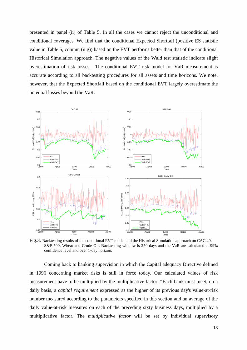
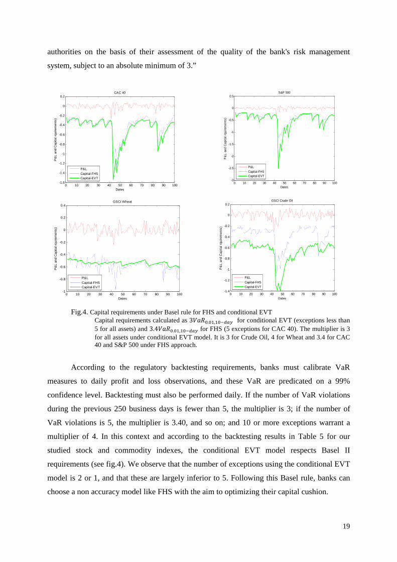
Fig.4. Capital requirements under Basel rule for FHS and conditional EVT Capital requirements calculated as 3BCD,.,�,�,��S� for conditional EVT (exceptions less than 5 for all assets) and 3.4BCD,.,�,�,��S� for FHS (5 exceptions for CAC 40). The multiplier is 3 for all assets under conditional EVT model. It is 3 for Crude Oil, 4 for Wheat and 3.4 for CAC 40 and S&P 500 under FHS approach.
According to the regulatory backtesting requirements, banks must calibrate VaR
measures to daily profit and loss observations, and these VaR are predicated on a 99%
confidence level. Backtesting must also be performed daily. If the number of VaR violations
during the previous 250 business days is fewer than 5, the multiplier is 3; if the number of
VaR violations is 5, the multiplier is 3.40, and so on; and 10 or more exceptions warrant a
multiplier of 4. In this context and according to the backtesting results in Table 5 for our
studied stock and commodity indexes, the conditional EVT model respects Basel II
requirements (see fig.4). We observe that the number of exceptions using the conditional EVT
model is 2 or 1, and that these are largely inferior to 5. Following this Basel rule, banks can
choose a non accuracy model like FHS with the aim to optimizing their capital cushion.
0 10 20 30 40 50 60 70 80 90 100-3
-2.5
-2
-1.5
-1
-0.5
0
0.5
Dates
P&
L an
d C
apita
l rqu
irem
ents
)
S&P 500
P&L
Capital-FHSCapital-EVT
0 10 20 30 40 50 60 70 80 90 100-1
-0.8
-0.6
-0.4
-0.2
0
0.2
0.4
Dates
P&
L an
d C
apita
l rqu
irem
ents
)
GSCI Wheat
P&L
Capital-FHSCapital-EVT
0 10 20 30 40 50 60 70 80 90 100-1.4
-1.2
-1
-0.8
-0.6
-0.4
-0.2
0
0.2
Dates
P&
L an
d C
apita
l rqu
irem
ents
)
GSCI Crude Oil
P&L
Capital-FHSCapital-EVT
0 10 20 30 40 50 60 70 80 90 100-1.6
-1.4
-1.2
-1
-0.8
-0.6
-0.4
-0.2
0
0.2
Dates
P&
L an
d C
apita
l rqu
irem
ents
)
CAC 40
P&L
Capital-FHSCapital-EVT
20
6. Conclusion
The estimation of the generalized Pareto distribution fitting the extreme returns allows
us to bring to light the existence of fat tails. So, the risk of extreme loss on stock and
commodity indexes is higher than the occurrence of expected gains. The study reveals that the
tails index of the generalized Pareto distribution on returns are generally positive. These
results particularly confirm the previous research results over 1-day horizon. We also find that
these results are valid over 5-day and 10-day horizons. The last time horizon allows
computing capital requirement over 10-day horizon.
Through backtesting procedures, the unconditional Historical Simulation fails to
accurately measure risk losses on the studied assets (CAC 40, S&P 500, Wheat and Crude
Oil). We observe strong underestimation of VaR and Expected Shortfall measures using
Historical Simulation approach. Comparatively, the unconditional EVT model performs better
at 5-day and 10-day horizons but less well at a 1-day horizon. For both the unconditional risk
models, the number of VaR violations decreases when the confidence level increases. The
underestimation also decreases when the time horizon rises.
We demonstrate in this study that introducing GJR-GARCH modeling in the EVT
model to compute conditional VaR is more reliable for measuring financial risks in normal
and abnormal market conditions. The backtesting results in panel (ii) of Table 5 show the
accuracy of our conditional EVT VaR measures for all studied assets. We note, however, a
strong overestimation for the Expected ShortFall measures based on the conditional EVT
model. Even in the 2008 financial crisis, the conditional EVT model is more accurate and
reliable for predicting the asset risk losses. We note the rules relating the capital multiplier to
the number of exceptions are arbitrary, and there are concerns that the high scaling factor
could discourage banks from developing and implementing best practices.
For future research, it would be interesting to broaden this study to multivariate EVT
modeling by taking into account asset correlation problems. Modeling stress testing using
EVT model is a challenging area in respect to the Basel III perspective.
21
Appendix A: standard Historical Simulation method
Let ��, ��, …, �� be as n random variables independently and identically distributed
measuring the daily returns of an investment at the moments 1, 2, n which is defined by the
unknown cumulative distribution function F. The VaR at α risk level can be defined by:
BCD� �� ��Ctzo�m �V�V+�� � (23)
where �� @ �� @ � @ ��
Expected Shortfall based on the historical simulation method is defined by:
O$� �� E�X/X � BCD� (24)
Appendix B: Filtered Historical Simulation method
The Filtered Historical Simulation approach combines the historical simulation and the conditional volatility models like GARCH. To estimate volatility, we use GJR-GARCH(1,1) model, which in addition to the characteristics of GARCH model, has a leverage effect (positive and negative return have different impact on volatility). This volatility can be obtained by:
=[,V� \, 5 \�XV��� 5 ] _`ab.,XV��� 5 \�=[,V��� (25)
Where ] reflects an asymmetric effect on volatility whether the last period random residuals was positive or negative.
The return is calculated with first-order autoregressive AR(1) model.
�V WV 5 XV WV 5 ZV=[,V (26)
WV Y, 5 Y��V�� (27)
where WV is the conditional mean. The parameters Y� and \� are derived from Maximum Likelihood Estimation.
To make residuals XV suitable for historical simulation, we divide residuals by conditional volatility forecast =V to obtain standardized residuals ZV.
ZV XV=[,V 28�
That series of standardized residuals are then updated with forecasted volatility =FV�� to obtain current market condition
22
ZV�� ZV=F[,V�� 29�
Simulated returns can be generated by:
�HV�� WV 5 ZV�� 30�
Therefore, we can calculate desired VaR in Eq. (23) and ES in Eq. (24) for each simulated return series at chosen confidence level. For a complete discussion on the use of historical simulation approach for VaR estimation, you can see various articles such as Hendriks (1996) and Barone-Adesi et al. (2000).
23
References
Alexander, C. and Sheedy, E. (2008), Developping a stress testing framework based on market risk models, Journal of Banking and Finance, 32, 2220-2236. Artzner, P. (2001), Application of coherent risk measures to capital requirements in
Insurance, North American Actuarial Journal, N° 3, 11-25. Artzner, P., Delbaen, F., Eber, J. M. and Heath, D. (1999), Coherent Measure of Risk,
Math. Fin, Vol. 9 (3), 203-228. Assaf, A. (2009), Extreme observations and risk assessment in the equity markets of MENA
region: Tail measures and Value-at-Risk, International review of Financial Analysis, N° 18, 109-116.
Balkena, A., De Haan, L. (1974), Residual life at great age, Annals of Probability 2, 792-804. Barone-Adesi, G., Bourgoin, F., Giannopoulos, K. (1998), Don’t look back, Risk 11, 100-103. Barone-Adesi, G., Giannopoulos, K., Vosper, L. (2000), Filtered Historical Simulation.
Backtest Analysis, University of Westminster. Basak, S., Shapiro, A. (2001), Value-at-risk-based risk management: optimal policies and
asset prices, Review of Financial Studies, 14, 371–405. Basel Committee on Banking Supervision, (1996), Amendement to the Capital Accord to
Incorporate Market Risks. Basel Committee on Banking Supervision, (2006), International Convergence of Capital
Measurement and Capital standards: A Revised Framework Comprehensive Version (Bank for International Settlements, Basel).
Bollerslev, T. (1986), Generalised autoregressive conditional heteroskedasticity, Journal of Econometrics, 31, 309-328.
Campbell, S.D. (2005), A review of backtesting and backtesting procedures. Finance and Economics Discussion Series Division of Research Statistics and Monetary. Affairs Federal Reserve Board, Washington, D.C.
Christoffersen, P., Hahn, J., Inaoue, A. (2001), Testing and comparing value-at-risk measures, Journal of Empirical Finance, 8, 325–342.
Coles, S. (2001), An Introduction to Statistical Modeling of Extreme Values, Spring series in statistics, Springer-Verlag London Limited.
Da Silva, A.C., and Mendez, B. V. D. M. (2003), Value at Risk and extreme Returns in Asian Stock Markets, International Journal of Business, 8, 17-40.
Dowd, K. (2005), Measuring market risk, Willey Finance. Embrechts, P. (2000), Extremes and Integrated Risk Management, published in association
with UBS Warburg and Risk Books. Embrechts, p., Kluperberg, C., Mikosch, T. (1997), Modeling Extremal Events for insurance
and finance, Springer. Embrechts, P., Resnick, C., Samorodnitsky, G. (1999), Extreme Value Theory as a Risk
Management Tool, North American Actuarial Journal, 3, 30-41. Embrechts, P., Kauffman, R., Patie, P. (2005), Strategic Long-Term Financial Risks: Single
Risk Factors, Computational Optimization and Applications, 32, 61-90. Engle, R.F., Manganelli, S. (1999), CAViaR : Conditional autoregressive value at risk by
regression quantiles, Journal of Business & Economic Statistics, 22, 367-381. Fernandez, V. (2003), Extreme value theory and value-at-risk, Departement of industrial
engineering at the University of Chile (DII). Fromont, E. (2005), Modélisation des rentabilités extrêmes des distributions des
Hedge,Funds, CREM UMR CNRS 6211- Axe Macroéconomie et Finance. Gencay, R., Selcuk, F. (2004), Extreme Value Theory and Value at Risk: Relative
Performance in Emerging Markets, International Journal of Forecasting, 20, 287-303. Haas, M. (2001), New methods in backtesting, Working paper, Financial engineering research
24
center caesar Bonn. Haas, M. (2005), Improved duration-based backtesting of value-at-risk, Working paper,
Institute of Statistics, University of Munich. Jorion, P. (2002), Value at Risk, Second edition, McGraw Hill, New York. Liang, B. (1999), On the Performance of hedge Funds, Journal of Finance and Quantitative
Analysis, 35, 383-408. Kupiec, P. (1995), Techniques for verifying the accuracy of risk management models, Journal
of Derivatives, 3, 73-84. Lopez, J. A. (1999), Regulatory evaluation of value-at-risk models, Journal of Risk, 1, 37-64. Longin, F. (1998), Value at Risk: Une nouvelle approche fondée sur les valeurs extrêmes,
Annales d’Economie et Statistiques, 52, 1-29. Longin, F. (2000), From value at risk to stress testing: the extreme value approach, Journal of
Banking and Finance, 24, 1097-1130. Longin, F. (2001), Beyond the VaR, The Journal of Derivatives, 8, 36-48. McNeil A.J., Frey, R. (2000), Estimation of tail-related risk measures for heteroscedastic
financial time series : an extreme value approach, Journal of Empirical Finance, 7, 271- 300.
Michell and Pulvino. (2000), Characteristics of risk in risk arbitrage, Working paper, Harvard. Nefci, S. (2000), Value at Risk Calculations, Extreme Events, and Tail Estimation, The
Journal of Derivatives, 1-15. Pickands, J. (1975), Statistical inference using extreme order statistics, Annals of Statistics, 3,
119-131. Reiss, R.D., Thomas, M. (2001), Statistical Analysis of Extreme Values: from Insurance,
Finance, Hydrology and Other Fields, Birkhauser Verlag, Basel. Rockafellar, R. T., Uryasev, S. (2001), Conditional VaR for general loss distributions,
Journal of Banking and Finance, 26(7), 1443-1471. Timotheos, A., Degiannakis, S. (2006), Backtesting VaR models: an expected shortfall
approach, Working paper, Athens University of Economics and Business. Velayoudoum, M., Bechir, R., Abdelwahed,T. (2009), Extreme Value Theory and Value at
Risk: Application to oil market, Energy Economics, 31, 519-530. Vladimir, O., et al. (2009), An application of EVT, GPD and POT methods in Russian market
Oryol Regional Academy of State Service, Oryol, 5.
Recommended