EXPERIMENTAL STUDY OF THE DEVELOPMENT FLOW REGION ON STEPPED CHUTES
by Rafael Eduardo Murillo - Muñoz A thesis submitted to the Faculty of Graduate Studies in partial fulfillment of the requirements for the degree of Doctor of Philosophy Department of Civil Engineering University of Manitoba Winnipeg, Manitoba, Canada February, 2006 © Rafael Eduardo Murillo-Muñoz, 2006
Experimental Study of the Development Flow Region on Stepped Chutes i
Abstract
The development flow region of stepped chutes was studied experimentally.
Three configuration of chute bed slopes 3.5 :1H V , 5 :1H V and 10 :1H V , were used to
study the flow characteristics. Each model had five horizontal steps and with constant
step height of 15 cm. Constant temperature anemometry was used to investigate the
velocity field characteristics as well as local void fraction. Pressure transducers were
used to examine the pressure distribution. The conditions of aerated and non-aerated
cavity were studied.
It was found that the temperature anemometry is a valuable tool in the study of
water flow problems due to its good spatial and temporal resolution. It is recommended
that the constant overheat ratio procedure should be used in dealing with non-isothermal
water flows.
Flow conditions along the development flow region were found to be quite
complex with abrupt changes between steps depending whether or not the flow jet has
disintegrated. The flow on this region does not resemble a drop structure and after the
first step, the step cavity condition does not affect the flow parameters.
Pressure distribution was also found to be complex. It was found that there are no
conclusive pressure profiles either on the step treads nor on step risers. No correlation
was observed with the values of pool depth.
The instantaneous characteristics of the velocity field along the jet of a drop
structure were also studied. It was concluded that the cavity condition does not affect the
velocity field of the sliding jet. The shear stress layer at the jet/pool interface was
quantified.

Experimental Study of the Development Flow Region on Stepped Chutes ii
Acknowledgments
This study was funded by Manitoba Hydro’s Research and Development Program
(Project G168), and the Natural Science and Engineering Research Council (NSERC),
Canada. The research was carried out at the Hydraulics Research and Testing Facility,
Civil Engineering Department, University of Manitoba.

Experimental Study of the Development Flow Region on Stepped Chutes iii
Table of contents
Abstract i
Acknowledgement ii
Table of contents iii
List of Figures viii
List of Tables xv
List of Symbols xv
Chapter 1 Introduction 1
1.1 Stepped chutes and cascades 1
1.2 Hydraulic expertise 3
1.2.1 Flow regimes in a stepped chute 4
1.3 Nappe flow regime 5
1.3.1 Onset conditions 5
1.3.2 Nappe flow sub-regimes 6
1.3.3 Flow development characteristics 7
1.4 Transition flow regime 8
1.4.1 Onset conditions 9
1.4.2 Transition flow sub-regimes 9
1.4.3 Flow development characteristics 9
1.5 Skimming flow regime 10
1.5.1 Onset conditions 11
1.5.2 Skimming flow sub-regimes 13

Experimental Study of the Development Flow Region on Stepped Chutes iv
1.5.3 Flow development characteristics 13
1.6 Stepped chutes with inclined steps 14
1.7 Objectives of the study 16
1.8 Structure of the report 16
Chapter 2 Experimental setting 21
2.1 Introduction 21
2.2 Model description 21
2.3 Instrumentation and data acquisition 23
2.3.1 Data acquisition system 24
2.3.2 Pressure measurement system 24
2.3.3 Velocity measurement 25
2.3.4 Other equipment 26
2.4 Instrument calibration 27
2.4.1 Pressure transducers 27
2.4.2 Constant temperature anemometer 28
2.5 Modeling conditions 29
2.6 Constant temperature anemometry 31
2.6.1 Two-phase flow measurements using CTA 32
2.6.2 Bubble detection method 34
2.6.3 Signal analysis 34
Experimental Study of the Development Flow Region on Stepped Chutes v
Chapter 3 Constant temperature anemometry compensation 42
3.1 Introduction 42
3.2 Temperature compensation 42
3.3 Constant sensor temperature procedure 43
3.4 Constant overheat ratio procedure 44
3.4.1 Heat transfer law 45
3.4.2 Sensitivity analysis 48
3.5 Buoyancy effects 49
3.6 Final comments 50
Chapter 4 Velocity and local void fraction observations 57
4.1 Introduction 57
4.2 Phase detection 57
4.3 Voltage correction 60
4.4 Experimental conditions 60
4.5 Flow description 61
4.6 Velocity observations 65
4.7 Local void fraction observations 66
Chapter 5 Pressure observations 93
5.1 Introduction 93
5.2 Step cavity observations 93
5.3 Pressure observation on step treads 95

Experimental Study of the Development Flow Region on Stepped Chutes vi
5.4 Pressure observation on step risers 98
5.5 Pool depths observations 100
Chapter 6 Drop structures observations 125
6.1 Introduction 125
6.2 Profile locations 125
6.3 Velocity observations 126
6.4 Local void fraction observations 130
Chapter 7 Summary and conclusions 142
7.1 Introduction 142
7.2 Summary 142
7.3 Conclusions 149
7.4 Future works 151
References 153
Appendix A Flow conditions for the runs 161
Appendix B Velocity field and local void fraction observations.
Model II. 170

Experimental Study of the Development Flow Region on Stepped Chutes vii
Appendix C Velocity field and local void fraction observations.
Model III. 196

Experimental Study of the Development Flow Region on Stepped Chutes viii
List of figures
Figure 1.1 Flow regimes on stepped spillways. a) Nappe flow regime b)
Transition flow regime. c) Skimming flow regime 17
Figure 1.2 Flow regimes criterion according to Yasuda and Ohtsu (1999) 18
Figure 1.3 Different step types: a) horizontal step, b) upward steps, c)
pooled steps 18
Figure 1.4 Nappe flow regime criteria 19
Figure 1.5 Nappe flow sub-regimes according to Chanson (2001e). a)
Nappe flowwith fully developed hydraulic jump (sub-regime NA1).
b) Nappe flow with partially-developed hydraulic jump (sub-regime
NA2) c) Nappe flow without hydraulic jump (sub-regime NA3) 20
Figure 2.1 General layout of the models 36
Figure 2.2 General overview of the models. a) Model I during construction.
b) Final layout of Model I. c) Model I during intial tests. d)
Overview of the three models 37
Figure 2.3 Linear response of the pressure transducers. Calibration of
March 15, 2005 38
Figure 2.4 Schematic diagram of the water tunnel 39
Figure 2.5 Measured H2 profiles on the approach channel 40
Figure 2.6 Schematic representation of a signal from a hot-film probe
immersed in a liquid flow with gas bubble 40
Figure 2.7 Schema of bubble detection method. a) Amplitude threshold. b)
slope threshold 41

Experimental Study of the Development Flow Region on Stepped Chutes ix
Figure 3.1 Calibration curves of a conical probe using the constant sensor
temperature procedure. Overheat ratio = 10% , 18.5setupT C= ° ,
15.53SR = ohms. 52
Figure 3.2 Variation of Nu with actual overheat ratio Θ 52
Figure 3.3 Variation of the conical probe cool resistance with temperature 53
Figure 3.4 Comparison of flow velocity, test G13 53
Figure 3.5 Schematic diagram of the manual adjustment of the overheat
ratio 54
Figure 3.6 Example of test results using the constant overheat ratio
technique 54
Figure 3.7 Fitting results of analytical functions, test H7 55
Figure 3.8 Variation of the CTA output with changes in decade resistance 55
Figure 3.9 Region of forced and free convection flow for a typical conical
hot-film probe operated with the constant overheat ratio technique.
Overheat ratio set at 10% 56
Figure 4.1 Selection of voltage threshold. a) histogram of CTA output
voltage b) autocorrelation plot 68
Figure 4.2 Selection of slope threshold. a) typical time series of CTA output
voltage b) slope of the CTA output signal 69
Figure 4.3 Correction of voltages. a) relationship between corrected voltage
and under-compensated (minus one) and over-compensate signal
(plus one) b) velocity profile before and after correction 63

Experimental Study of the Development Flow Region on Stepped Chutes x
Figure 4.4 Step cavity conditions on Model II. a) step1, aerated. b) step1,
non-aerated. c) step2, aerated. d) step2, non-aerated. 71
Figure 4.5 Step cavity conditions on Model III. a) step1, aerated. b) step1,
non-aerated. c) step2, aerated. d) step2, non-aerated. 72
Figure 4.6 Nappe flow regime on Model II. Non-aerated step cavity,
0.51cy h = . a) step 1. b) step2. c) step 3. d) step 4 73
Figure 4.7 Nappe flow regime on Model III. Arated step cavity,
0.49cy h = . a) step 1. b) step2. c) step 3. d) step 4 74
Figure 4.8 Transition flow regime on Model II. Non-aerated step cavity,
1.01cy h = . a) step 1. b) step2. c) step 3. d) step 4 75
Figure 4.9 Transition flow regime on Model III. Aerated step cavity,
1.09cy h = . a) step 1. b) step2. c) step 3. d) step 4 73
Figure 4.10 Entrainment of air into the step cavity. Model III, 1.09cy h = ,
step 2. Imagines approximately every 0.4 seconds 77
Figure 4.11 Skimming flow regime on Model II. Non-aerated step cavity,
1.66cy h = . a) step 1. b) step2. c) step 3. d) step 4 78
Figure 4.12 Skimming flow regime on Model III. Aerated step cavity,
1.66cy h = . a) step 1. b) step2. c) step 3. d) step 4 79
Figure 4.13 Shock waves at skimming flow regime. a) Model II. b) Model
III 80
Figure 4.14 Velocity profiles at step brink, 5L h = . Model II 81
Figure 4.15 Velocity profiles at step brink, 10L h = . Model III 82

Experimental Study of the Development Flow Region on Stepped Chutes xi
Figure 4.16 Comparison of velocity profiles with aerated flows at step
brinks. Model II at 5L h = , Model III at 10L h = 83
Figure 4.17 Comparison of velocity profiles with non-aerated flows at step
brinks. Model II at 5L h = , Model III at 10L h = 84
Figure 4.18 Velocity profiles at transition flow regime 85
Figure 4.19 Velocity profile at skimming flow regime 86
Figure 4.20 Local void fraction profiles at step brink, 5L h = . Model II 87
Figure 4.21 Local void fraction profiles at step brink, 10L h = . Model III 88
Figure 4.22 Comparison of local void fraction profiles with aerated flows at
step brinks. Model II at 5L h = , Model III at 10L h = 89
Figure 4.23 Comparison of local void fraction profiles with non-aerated
flows at step brinks. Model II at 5L h = , Model III at 10L h = 90
Figure 4.24 Local void fraction profiles at transition flow regime 91
Figure 4.25 Local void fraction profile at skimming flow regime 92
Figure 5.1 Observed points were the air pocket vanishes. Aerated
conditions: runs A8, B15-B18 and C1. Non-aerated condition: runs
A7, B1 and C1 102
Figure 5.2 Slope effect on the presence of the air pocket. Constant step
height of 15 cm 103
Figure 5.3 Observed average pressure along Step 1 on Model I. Aerated
condition: run A3, A11 to A13; non-aerated: run A4 104
Figure 5.4 Measured average pressure on step treads on Model II. Aerated
condition: Run B11 to B14; non-aerated condition: runs B7 to B10 105
Experimental Study of the Development Flow Region on Stepped Chutes xii
Figure 5.5 Measured average pressure on step treads on Model III. Aerated
condition: Run C11 to C14; non-aerated condition: runs C7 to C10 106
Figure 5.6 Recorded pressure on the treads of Model I, aerated flow
condition 107
Figure 5.7 Average pressure on the treads of Model II. Aerated cavity:
figures a to c; non-aerated cavities: figures d to f 108
Figure 5.8 Average pressure on the treads of Model III. Aerated cavity:
figures a to c; non-aerated cavities: figures d to f 109
Figure 5.9 Average pressure on the tread of step 1 110
Figure 5.10 Average pressure on the tread of step 2 111
Figure 5.11 Average pressure on the tread of step 3 112
Figure 5.12 Average pressure on the tread of step 4 113
Figure 5.13 Average pressures on the riser of step 1, Model I. Aerated step
cavity: run A1; non-aerated step cavity: run A2 114
Figure 5.14 Average pressures on risers of Model II. Aerated step cavity:
runs B15-B18; non-aerated step cavity: runs B3- B6 115
Figure 5.15 Average pressures on risers of Model III. Aerated step cavity:
runs C15-C18; non-aerated step cavity: runs C3- C6 116
Figure 5.16 Average pressure on the risers of Model I. Condition of the step
cavity: aerated 117
Figure 5.17 Average pressure on the risers of Model II. Aerated step cavity:
Figures a to c; non-aerated step cavity: figures d to f 118

Experimental Study of the Development Flow Region on Stepped Chutes xiii
Figure 5.18 Average pressure on the risers of Model III. Aerated step
cavity: Figures a to c; non-aerated step cavity: figures d to f 119
Figure 5.19 Average pressure on the riser of step 1 120
Figure 5.20 Average pressure on the riser of step 2 121
Figure 5.21 Average pressure on the riser of step 3 122
Figure 5.22 Average pressure on the riser of step 4 123
Figure 5.23 Correlation between water pool levels and discharge. Condition
of the step cavity: aerated 124
Figure 6.1 Flow geometry at a drop structure. a) aerated step cavity; b) non-
aerated step cavity 131
Figure 6.2 Velocity profiles on the midsection of the sliding jet. a) Aerated
flow; b) fully depleted nappe; c) low discharge, d) large discharge. 132
Figure 6.3 Velocity gradient profiles on the midsection of the sliding jet. a)
Aerated flow; b) fully depleted nappe; c) low discharge, d) large
discharge. 133
Figure 6.4 Turbulence intensity profiles on the midsection of the sliding jet.
a) Aerated flow; b) fully depleted nappe; c) low discharge, d) large
discharge. 134
Figure 6.5 Normal stress profiles on the midsection of sliding jet. a)
Aerated flow; b) fully depleted nappe; c) low discharge, d) large
discharge. 135
Figure 6.6 Velocity profiles along the jet trajectory. a) upstream brink; c)
free falling jet; c) sliding jet, d) toe of sliding jet. 136

Experimental Study of the Development Flow Region on Stepped Chutes xiv
Figure 6.7 Velocity gradient profiles along the jet trajectory. a) upstream
brink; b) free falling jet; c) sliding jet, d) toe of sliding jet. 137
Figure 6.8 Turbulence intensity profiles along the jet trajectory. a) upstream
brink; b) free falling jet; c) sliding jet, d) toe of sliding jet. 138
Figure 6.9 Normal stress profiles along the jet trajectory. a) upstream brink;
b) free falling jet; c) sliding jet, d) toe of sliding jet. 139
Figure 6.10 Local void fraction. a) midsection of sliding jet. 140
Figure 6.11 Chord length distribution at midsection (a and c) and
intersection line (b) of the sliding jet. 141
Experimental Study of the Development Flow Region on Stepped Chutes xv
List of Tables
Table 2.1 Hydraulic parameters for minimum and maximum flow 23
Table 2.2 Modeling conditions on the stepped chutes. Regime flow defined
according to Chanson and Toombes (2004). Discharge in m s 30
Table 3.1 Sum of the squared error for the 12 tests 48
Table 3.2 Variation of the CTA output voltage with a unit change in decade
resistance 49
Table 5.1 Location of pressure ports on step treads 96
Table 5.2 Location of pressure ports on the step risers 99

Experimental Study of the Development Flow Region on Stepped Chutes xvi
List of symbols
oA [-] regression coefficient
1A [-] regression coefficient
2A [-] regression coefficient
1d [m] water depth immediately after the jet impact
E [V] anemometer output voltage
AE [V] output voltage at AT
refE [V] output voltage at refT
Fr [-] Froude number
Gr [-] Grashof number
g [m/s2] acceleration due to gravity
h [m] step height
j [-] index
k [-] index, total number of points on the liquid phase
L [m] step length
iL [m] distance along the step tread measured from the step riser
N [-] total number of steps, total number calibration values
Nu [-] Nusselt number
n [-] exponent, number of points on the liquid phase
P [Pa] pressure
Q [m3/s] flow discharge

Experimental Study of the Development Flow Region on Stepped Chutes xvii
ER [-] Reynolds number
oR [ohms] sensor cold resistance
sR [ohms] sensor operating resistance
s [m] chord size
T [s] total time
AT [°C] water temperature
refT [°C] reference temperature
sT [°C] sensor temperature
setupT [°C] sensor temperature at setup
Tu [-] turbulence intensity
ABt [s] time interval between point A and B
U [m/s] flow velocity
avgU [m/s] depth average flow velocity
cU [m/s] calculated flow velocity
mU [m/s] measured flow velocity
u [m/s] instantaneous water velocity values,
2u [m2/s2] normal stress
We [-] Weber number
y [m] water depth
cy [m] critical water depth
jety [m] thickness of the water jet

Experimental Study of the Development Flow Region on Stepped Chutes xviii
py [m] water depth behind the overfalling jet
Ty [m] total water depth
*y [m] distance along the step riser measured upwards from the tread
α [-] void fraction
γ [N/m3] specific weight of water
ε [-] squared error
θ [degrees] chute slope
Θ [-] overheat ratio
φ [m] pipe diameter

Introduction
Experimental Study of the Development Flow Region on Stepped Chutes 1
Chapter 1 Introduction
The hydraulics of stepped spillways is a field that has evolved in the last 25 years
in direct connection with new construction techniques and new materials. Nevertheless,
it has been in the last decade that three possible flow regimes on a stepped spillway have
been clearly identified: the nappe, the transition, and the skimming flow regimes. Each
one of these regimes has different hydraulic properties and characteristics not yet well
understood, which makes the subject challenging for hydraulic engineers. In addition,
stepped spillways have proved to be an economic alternative for many dams and its
environmental benefits have just begun to be explored.
1.1 Stepped chutes and cascades
For the last few decades, stepped spillways have become a popular method for
handling flood releases. The key characteristic of them is the configuration of the chute,
which is made with a series of steps from near the crest to the toe. These steps increase
Introduction
Experimental Study of the Development Flow Region on Stepped Chutes 2
significantly the rate of energy dissipation taking place along the spillway face and
reduce the size and the cost of the downstream stilling basin.
Stepped chutes have been used for centuries. Applications can be found in the
ancient dams in the Khosr River (Iraq), in the Roman Empire, and in the Inca Empire
among other cultures. Chanson (1995a, 1995b, 1998, 2000, 2001c) presented an
interesting recompilation on the history of stepped spillways and cascades.
The recent popularity of stepped spillways is based on the development of new
construction materials, e.g., roller compacted concrete (RCC) and gabions among others.
The construction of a stepped spillway is compatible with RCC placement methods and
slip-forming techniques. Also stepped spillways are the most common type of spillways
used for gabion dams. Soviet engineers developed the concept of an overflow earthen
dam. In this type of structure, the spillway consists of a revetment of precast concrete
blocks with steps, which lays on a filter and erosion protection layer.
Stepped spillways are also utilized in water treatment plans. As an example, five
artificial cascades were designed along a waterway system to help the re-oxygenation of
the polluted canal (Macaitis, 1990; Robison, 1994). Stepped chutes and cascades have
also been used with aesthetic purposes. Examples can be found in the aqueducts of the
Roman Empire, in the Renaissance palaces of France, and in the modern Hong Kong
architecture among other places. Chanson (1998, 2001b) discussed this application in
detail.
Over the past decade, several dams have been built with overflow-stepped
spillway around the world: Clywedog dam (U.K.), La Grande 2 (Canada), Monksville
dam (U.S.A.), and Zaaihoek dam (South Africa) are a few examples.

Introduction
Experimental Study of the Development Flow Region on Stepped Chutes 3
1.2 Hydraulics expertise
In spite of the fact that examples of stepped chutes and cascades are present in
many ancient civilizations, there are not many references about them. Perhaps, the oldest
modern reference about stepped spillways is Wegmann (1907), who described the design
of the New Croton Dam, U.S.A. The next known references are given by Poggi (1949,
1956) and Horner (1969). Later on, Essery and Horner (1978) did a significant study to
quantify the energy dissipation and to describe the nappe and skimming flow regimes.
With the introduction of RCC dams during the 1980’s, stepped chutes regained
popularity and its literature revitalized (Young, 1982; Sorensen, 1985; Houston and
Richardson, 1988). Since then, many researchers (Diez-Cascon et al., 1991; Chanson,
1993, Chamani, 1997; Boes, 1999; among many others) have investigated the hydraulic
characteristics of such chutes; investigations that eventually led to the first international
workshop of stepped spillways held in Switzerland in March 2000 (Minor and Hager,
2000). All these efforts have shown that stepped chute flows can be divided into three
regimes: nappe flow for low discharges, transition flow for intermediate discharges, and
skimming flow for large discharges.
Of the three flow regimes, the skimming flow has captured the attention of most
of the studies. Research on the transition and nappe flow regimes is scarce. Descriptions
of the transition flow regime can be found in Ohtsu and Yasuda (1997), Chanson (2001a,
b), Chanson and Toombes (2001, 2004) as well as De Marinis et al. (2001). On the other
hand, Horner (1969), Essery and Horner (1978), Peyras et al. (1991, 1992) as well as
Chanson (1995a, 2001c) amongst others described some aspects of the nappe flow

Introduction
Experimental Study of the Development Flow Region on Stepped Chutes 4
regime. Chanson (1999a) used the drop structure’s concept to study the flow in the nappe
flow regime and Chanson and Toombes (1998a, b) reported experiments with
supercritical flow on a single step. Pinhero and Fael (2000) studied the energy
dissipation process and more recently Aigner (2001) utilized sharp-crested weirs to create
a nappe flow regime in pooled steps. Finally, El-Kamash et al. (2005) studied the bubble
characteristics in the two phase flow of the nappe flow regime. A brief description of the
three regimes follows.
1.2.1 Flow regimes in a stepped chute
As mentioned before, stepped chutes can present three flow regimes: nappe,
transition and skimming. In the nappe flow regime each step always has a falling nappe,
and an air pocket can be observed in the step cavity (Figure 1.1a), i.e., the step cavity is
fully aerated. In the transition flow (Figure 1.1b) air pockets are formed in some steps,
and recirculating vortices are formed in the other steps. This regime is characterized by
strong hydrodynamic fluctuations (Ohtsu and Yasuda, 1997) and nappe stagnation on
each horizontal face associated with a downstream spray (Chanson, 2001c).
Finally, in the skimming flow regime the air pocket is filled with water and
recirculating vortices are always presented at each step (Figure 1.1c). In this regime the
water flows over a pseudo bottom formed by the vortices and huge amounts of air are
entrained, therefore it is considered to be two-phase flow. Clear boundaries between the
three regimes have not been established yet. Rajaratnam (1990), Chamani and
Rajaratnam (1999), Yasuda and Ohtsu (1999), Minor and Boes (2001), Chanson and
Toombes (2004) as well as Ohtsu et al. (2004) have proposed expressions for the

Introduction
Experimental Study of the Development Flow Region on Stepped Chutes 5
boundary between transition and skimming flow regimes. Similarly, a few expressions
for the boundary between nappe and transition flow regimes have been proposed; these
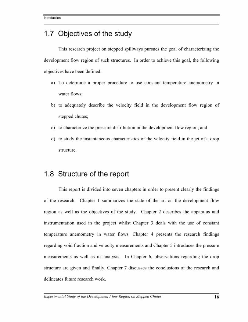
will be discussed in §1.3. As an example of the available criteria, Figure 1.2 presents the
boundaries for the three regimes as defined by Yasuda and Ohtsu (1999). In this figure
h is the step height, L is the step length and cy is the critical water depth.
1.3 Nappe flow regime
Chanson (2001c) defines the nappe flow regime as a succession of free falling
nappes and jet impacts from one step onto the next one when the step cavity is fully
aerated. This regime occurs at low discharges and it is characterized by the free falling
nappe at the upstream end of each step, an air cavity, and a pool of recirculating water.
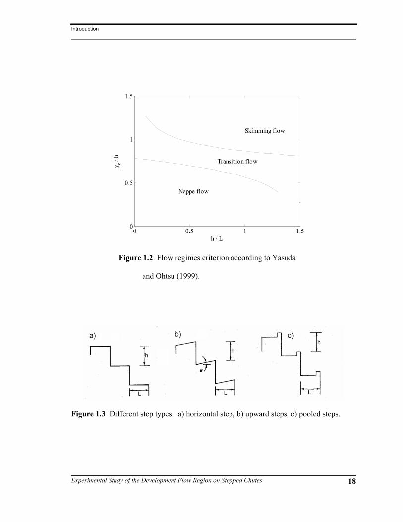
The geometry of the step can be horizontal, inclined (upward or downward) or pooled
(Figure 1.3). In the following paragraphs the state-of-the-art on the nappe flow regime is
summarized.
1.3.1 Onset conditions
The required hydraulic conditions to establish the nappe flow regime in a stepped
chute have not been clarified yet. Using experimental data available in the literature,
Rajaratnam (1990) proposed that values of 0.80cy h > will produce skimming flow in
the range 0.421 0.842h L≤ ≤ leaving the nappe flow regime when 0.80cy h ≤ .
Stephenson (1991), using the experience of South Africa dams, suggested that the most
suitable conditions for nappe flow situations are

Introduction
Experimental Study of the Development Flow Region on Stepped Chutes 6
1tan5
hL
θ = < , (1.1)
and
13
cyh< . (1.2)
Neither author considered transition flow regime.
Yasuda and Ohtsu (1999) considered the minimum step height required to form
the nappe flow. They expressed the boundary between nappe and transition flows as
( ) 0.261.4 1.4 tanc
hy
θ −= − . (1.3)
Chanson and Toombes (2004) proposed that the same boundary is given by
0.9174 0.381cy hh L= − , (1.4)
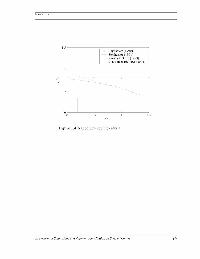
for the range 0 1.7h L≤ ≤ . All of the above expressions were developed for horizontal
steps and they are presented in Figure 1.4. This figure indicates that Stephenson (1991)
gives the more conservative criterion while Rajaratnam (1990) is the least conservative.
Yasuda and Ohtsu (1999) fairly agree with Chanson and Toombes (2004) on the
boundary between the nappe and transition flow regimes.
1.3.2 Nappe flow sub-regimes
In the case of chutes with horizontal steps, Horner (1969) as well as Essery and
Horner (1978) described two types of nappe flow: the isolated nappe flow and the nappe
interference flow. In the former, the nappe wholly strikes the tread of the step
immediately below and it occurs at low discharges. In the latter, the nappe overshoots

Introduction
Experimental Study of the Development Flow Region on Stepped Chutes 7
the tread section of the step and collides with the jet leaving this step. In both cases, the
water flow is supercritical along the entire cascade.
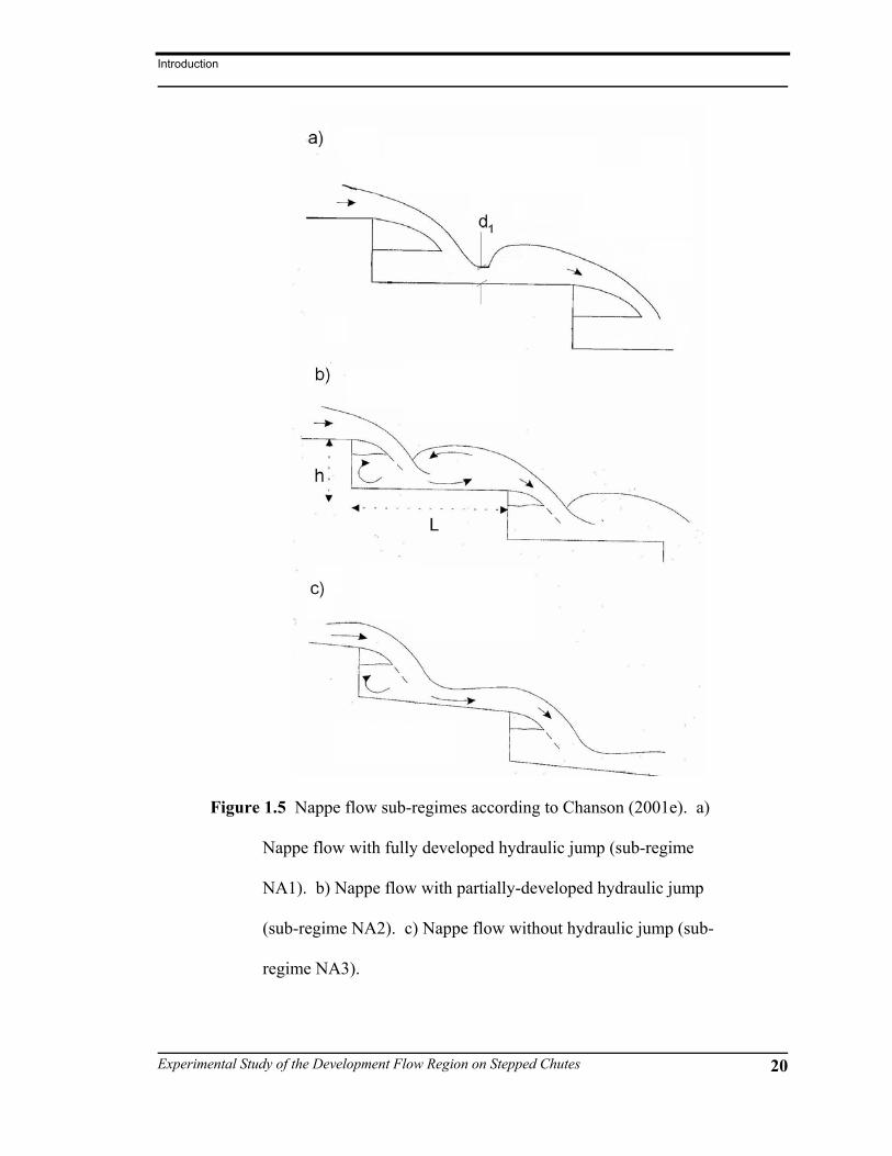
On the other hand, Chanson (2001c) suggested the existence of three nappe flow
sub-regimes: a) nappe flow with fully developed hydraulic jump (sub-regime NA1), b)
nappe flow with partially developed hydraulic jump (sub-regime NA2) and, c) nappe
flow without hydraulic jump (sub-regime NA3). Figure 1.5 gives a representation of
each sub-regime.
In the sub-regime NA1, the flow is critical at the step edge, supercritical in the
free falling nappe up to the hydraulic jump, and subcritical downstream of the jump and
up to the edge. On the other hand, in the NA2 sub-regime the hydraulic jump interferes
with the downstream step edge, and in sub-regime NA3 the flow is supercritical at any
position (Chanson, 2001c). Chanson (1994) determined that sub-regime NA2 occurs for
values of cy h smaller than a critical value given by
1.276
0.0916cy hh L
− <
, (1.5)
in the range 0.2 6h L≤ ≤ .
1.3.3 Flow development characteristics
Horner (1969) mentioned that as the flow enters a chute with a given step
geometry the stream accelerates and becomes fragmented on the initial reach of the
structure. He described this zone of the cascade as the transitory zone. Furthermore,
Horner pointed out that on steps lower down an equilibrium state is reached and flow
geometry is the same at each step. He referred to this section as the uniform flow.

Introduction
Experimental Study of the Development Flow Region on Stepped Chutes 8
Essery and Horner (1978) added to the uniform flow description that the flow geometry is
the same at each step but the depth varies across each one. Finally, Horner concluded
that the only flow not behaving in the manner outlined above are subcritical nappe flows
on inclined step cascades, which will be introduced in §1.6.
The length of the transitory zone is influenced by discharge per unit of width,
overall slope, step shape and step size, geometry of the spillway crest and the presence of
piers and gates (Horner, 1969). On the other hand, the most striking features of the
uniform flow are high velocities and fragmentation of the nappe (Horner, 1969).
In contrast to the above, Chanson (2001c) described two regions in nappe flows
without hydraulic jump (NA3 sub-regime): the flow establishment region and the
gradually varied flow region. The flow establishment region occurs on the first few steps
and it is characterized by three dimensional flow patterns, e.g., shock waves, and sidewall
standing waves (Chanson, 2001c). In the gradually varied flow region the flow patterns
are nearly identical from one step to another and a significant amount of air is entrained.
1.4 Transition flow regime
The transition flow regime is an intermediate stage between the nappe and the
skimming flow regimes. It appears at medium flows and it does not present the
succession of free jets observed in nappe flow nor the quasi-smooth free surface of
skimming flow. Nappe stagnation on each step and significant downstream spray are the
main characteristics of this flow regime.

Introduction
Experimental Study of the Development Flow Region on Stepped Chutes 9
1.4.1 Onset conditions
As discussed in §1.3, the onset conditions for nappe flow regime are not well
defined yet. Hence, the conditions for the transition flow regime have not been
established as well. Similarly, the boundary between the transition and the skimming
flow is still under study as it will discussed in §1.5.
1.4.2 Transition flow sub-regimes
Two sub-regimes in transition flow have been cited by Chanson and Toombes
(2004). The authors mentioned a lower range of transition flows with a longitudinal flow
pattern characterized by an irregular alternance of small to large air cavities downstream
of the inception point of the free surface aeration. They designated these ranges of flow
as the first sub-regime. On the other hand, the second sub-regime corresponded to the
upper range of transition flow rates in which the longitudinal flow pattern is characterized
by an irregular alternance of air cavities (small to medium) and filled cavities.
1.4.3 Flow development characteristics
The flow development characteristics on the transition flow are not clear yet.
Chanson (2001a) indicated that on flat slopes the flow in the development region is very
chaotic and it is characterized by significant changes in flow properties from one step to
the next one. The author mentioned that downstream, the flow becomes gradually varied
with slow variations of the flow properties from step to step, along with significant
longitudinal variations on each step. At the upstream end of the step, the flow is

Introduction
Experimental Study of the Development Flow Region on Stepped Chutes 10
characterized by a pool of recirculating water, stagnation and significant spray and water
deflection immediately downstream.
On a steep slope, Chanson (2001c) indicated that the upstream flow is smooth and
transparent. In the first few steps, the free surface is undular in phase with the stepped
geometry and some aeration in the step corners is observed immediately upstream of the
inception point (Chanson, 2001c). Downstream of this point, significant splashing is
observed.
1.5 Skimming flow regime
There is general agreement that the skimming flow regime appears once the step
cavity is filled with water and it cushions the flow. Thus, the external edges of the steps
form a pseudo-bottom over which the flow passes and stable recirculating vortices
develop between steps (Figure 1.1c). These vortices are maintained through the
transmission of shear stress from the fluid flowing past the edges of the steps and they are
believed to be responsible for the large energy dissipation that characterizes this regime.
For a stepped spillway with the skimming flow regime, the free surface of the
flow is smooth in the early steps and no air entrainment occurs in this region. This zone
occurs near the crest and it is distinguished by the presence of clear water. Next to the
boundary however, turbulence is generated. When the outer edge of the turbulent
boundary layer reaches the free surface, air entrainment at the free surface occurs. The
point where this phenomenon occurs is known as the point of inception. Downstream of
this point, a layer containing a mixture of both air and water extends gradually through

Introduction
Experimental Study of the Development Flow Region on Stepped Chutes 11
the fluid producing a region of gradually varied flow. Far downstream, the flow becomes
uniform and this reach is defined as the uniform equilibrium flow region.
1.5.1 Onset conditions
For small discharges and flat slopes, the water flows as a succession of waterfalls
(i.e., nappe flow regime). A small increase in discharge or slope might induce the
formation of transition flow regime and, if the discharge or the slope is further increased,
the skimming flow regime will develop. The onset of skimming flow is a function of the
discharge, the step height, and step length.
Several authors have studied the onset of the skimming flow regime. Rajaratnam
(1990) proposed that skimming flow appears once /cy h > 0.8. Chanson (1996) defined
the “onset of skimming flow” by the disappearance of the cavity beneath the free falling
nappes, and hence, the water flowing as a quasi-homogeneous stream. According to
Chamani and Rajaratnam (1999), the expression proposed by Chanson (1996) predicts
much larger values of /cy h , especially for h L greater than about 1.0. Furthermore,
they mentioned that during their experiments it was noted that, at the onset of skimming
flow the air pockets under the jet did not disappear. Thus, although the flow skims over
the steps, the recirculating flow did not fill the pockets under the jet. They argued that
this observation is contrary to the underlying assumption of Chanson (1996). Therefore,
Chamani and Rajaratnam (1999) proposed a different criterion based on visual
observations and assuming that the jet is parallel to the slope of the stepped spillway.
Their criterion is

Introduction
Experimental Study of the Development Flow Region on Stepped Chutes 12
1 0.34
0.89 1.5 1c cy yhL h h
− − = − + −
. (1.6)
According to Chamani and Rajaratnam (1999), prediction of Equation (1.6) is
generally good for h L greater than about 1.0, which is applicable for steeply sloped
stepped spillways. Furthermore, they suggested that the inner side of the jet just hits the
edge of the steps when
0.62
0.405 cyhL h
− =
. (1.7)
Moreover, James et al. (1999) indicated that skimming flow appears once /cy h is
larger than
1.07
0.541cy hh L
− =
, (1.8)
for 0.84h L < . Yasuda and Ohtsu (1999) give the step height for the formation of the
skimming flow as
( )0.1651.16 tanc
hy
θ= , (1.9)
in the region 0.1 ≤ tanθ ≤1.43, 0 ≤ / ch y ≤ 1.4, 5 ≤ /dam cH y ≤ 80. Boes, cited by Boes
and Minor (2000), indicated that skimming flow sets in for ratios larger than
0.91 0.14 tancyh
θ= − . (1.10)
A general agreement on the boundary between the transition and the skimming
flow has not been yet achieved. Yet, the best practice is to choose the criterion that best
fits the specific designing conditions.

Introduction
Experimental Study of the Development Flow Region on Stepped Chutes 13
1.5.2 Skimming flow sub-regimes
Chanson (2001c) distinguished three skimming flow sub-regimes depending on
the slope of the spillway. On flat slopes, the author mentioned the wake-step interference
and the wake-wake interference sub-regimes. The first sub-regime is characterized by
the fact that the wake does not cover completely the step tread and a three-dimensional
unstable recirculation is present in it. On the other hand, the main characteristic of the
second sub-regime is that the length of the wake and step tread is approximately the same,
therefore there is some interference between one step and the next one. Finally, on steep
slopes, Chanson (2001c) mentioned the recirculating cavity flow sub-regime. In this sub-
regime, the recirculating flow appears asymmetrical with most vorticity activity
occurring in the downstream part of the cavity.
1.5.3 Flow development characteristics
On a stepped chute, the flow can be subdivided into so-called clear water and
white water regions. Starting from the crest to the inception point, a clear water region
may be observed, whereas the white water region develops in the downstream portion
with the characteristic two-phase air-water flow. The critical depth mainly governs the
clear water region, while the uniform aerated flow depth has a significant effect on the
white water region.
The flow in the clear water region always has a drawdown curve due to the
transition from sub- to supercritical flow on the spillway crest. In contrast, the air-water
mixture flow always has a backwater curve due to the entrainment of air and the resulting

Introduction
Experimental Study of the Development Flow Region on Stepped Chutes 14
flow bulking. Therefore, for a very long stepped spillway of constant slope, there exist
three characteristic flow depths:
a) the critical depth at the spillway crest,
b) the inception depth (a local minimum), and
c) the uniform aerated depth (asymptotic maximum).
The transitions between these three characteristics flow depths are the drawdown
and the backwater curves. Hager and Boes (2000) presented expression for both curves.
1.6 Stepped chutes with inclined steps
Stepped chutes and cascades with inclined steps have not been studied in detail.
Horner (1969), Essery and Horner (1978), Peyras et al. (1991, 1992), Chanson (2001c)
discussed some experimental results with inclined steps. Horner (1969) concluded that
flow behavior on inclined steps falls into two categories: that in which the approach flow
to each drop is subcritical, and that in which it is supercritical. He also observed a
transition category in which both states of flow occurred.
The subcritical category was observed by Horner (1969) at relative low
discharges and it was characterized by subcritical pools on all the step surfaces (Horner,
1969). The flow leaving the steps passed from the subcritical flow state through critical
depth and into the supercritical nappes. Further downstream, the flow changes from
supercritical to subcritical by means of a hydraulic jump. According to Horner, little or
no fragmentation of the nappe occurs with flows of the subcritical category and the
uniform zone may be considered to extend over the whole of the cascade. On the other

Introduction
Experimental Study of the Development Flow Region on Stepped Chutes 15
hand, the transitory category is characterized by supercritical flow in the transitory zone
and subcritical flow in the uniform zone (Horner, 1969).
In the supercritical category flow behavior is similar to that on a cascade of
horizontal steps (Horner, 1969). That is, conditions are everywhere supercritical and the
flow passes through a transitory zone before equilibrium is established in a uniform zone.
At any discharge, the number of steps on an inclined step cascade over which the
transition zone forms is less than the number on a horizontal step cascade with the same
overall slope and step size (Essery and Horner, 1978).
Horner (1969) also considered the influence of nappe ventilation on the flow
conditions. In the case of flow in the subcritical category his investigation revealed that
the effect of aeration on flow behavior of a cascade was similar to the influence at a
single drop. That is to say on a cascade with no air vents the pressure beneath the nappes
became sub-atmospheric. With flows in the supercritical category, however, Horner
concluded that there was no marked difference between the uniform zone flow patterns
created on cascades with and without ventilation. Horner pointed out that the reason for
this was the highly fragmented nature of the stream after the first few steps, and the
consequent provision of an adequate supply of air through the nappes.
Finally, Peyras et al. (1991, 1992) observed an NA1 sub-regime on an upward
inclined step and pooled step chutes at low discharges only. They applied Rand’s (1955)
expressions and concluded that these expressions can be used on inclined steps as
preliminary computations. Peyras et al. performed their experiments on stepped gabion
weirs.
Introduction
Experimental Study of the Development Flow Region on Stepped Chutes 16
1.7 Objectives of the study
This research project on stepped spillways pursues the goal of characterizing the
development flow region of such structures. In order to achieve this goal, the following
objectives have been defined:
a) To determine a proper procedure to use constant temperature anemometry in
water flows;
b) to adequately describe the velocity field in the development flow region of
stepped chutes;
c) to characterize the pressure distribution in the development flow region; and
d) to study the instantaneous characteristics of the velocity field in the jet of a drop
structure.
1.8 Structure of the report
This report is divided into seven chapters in order to present clearly the findings
of the research. Chapter 1 summarizes the state of the art on the development flow
region as well as the objectives of the study. Chapter 2 describes the apparatus and
instrumentation used in the project whilst Chapter 3 deals with the use of constant
temperature anemometry in water flows. Chapter 4 presents the research findings
regarding void fraction and velocity measurements and Chapter 5 introduces the pressure
measurements as well as its analysis. In Chapter 6, observations regarding the drop
structure are given and finally, Chapter 7 discusses the conclusions of the research and
delineates future research work.

Introduction
Experimental Study of the Development Flow Region on Stepped Chutes 17
Figure 1.1 Flow regimes on stepped spillways. a) Nappe
flow regime. b) Transition flow regime. c)
Skimming flow regime.
Introduction
Experimental Study of the Development Flow Region on Stepped Chutes 18
0 0.5 1 1.50
0.5
1
1.5
y c / h
h / L
Skimming flow
Transition flow
Nappe flow
Figure 1.2 Flow regimes criterion according to Yasuda
and Ohtsu (1999).
Figure 1.3 Different step types: a) horizontal step, b) upward steps, c) pooled steps.
Introduction
Experimental Study of the Development Flow Region on Stepped Chutes 19
0 0.5 1 1.50
0.5
1
1.5
y c / h
h / L
Rajaratnam (1990)Stephenson (1991)Yasuda & Ohtsu (1999)Chanson & Toombes (2004)
Figure 1.4 Nappe flow regime criteria.
Introduction
Experimental Study of the Development Flow Region on Stepped Chutes 20
Figure 1.5 Nappe flow sub-regimes according to Chanson (2001e). a)
Nappe flow with fully developed hydraulic jump (sub-regime
NA1). b) Nappe flow with partially-developed hydraulic jump
(sub-regime NA2). c) Nappe flow without hydraulic jump (sub-
regime NA3).

Experimental setting
Experimental Study of the Development Flow Region on Stepped Chutes 21
Chapter 2 Experimental setting
2.1 Introduction
This chapter presents the characteristics of the models used during the
experimental work of this study. It also describes the instrumentation and data
acquisition systems employed throughout the project. Descriptions of the calibration
procedures and modeling conditions are also included as well as theoretical
considerations about constant temperature anemometry. Factors affecting such a
technique as well as its use in two phase flow measurements is also described.
2.2 Model description
Three models of a stepped chute were built at the Hydraulics Research & Testing
Facility (HRTF), University of Manitoba. The models were made of High Density
Overlay (HDO) plywood and they consist of three sections: a forebay, an approach
channel and the stepped chute (Figures 2.1). The forebay was a box of
31.22 2.44 1.22 m× × where perturbations, produced by the discharge of pressure flow
Experimental setting
Experimental Study of the Development Flow Region on Stepped Chutes 22
from the supply line, were dissipated. The approach channel was 7.32 m in length, with
a rectangular cross section ( )20.412 0.610 m× and a horizontal slope. Due to space
limitations at the time of construction, the channel intake had an angle of 45° with
respect to the head tank as well as a 45° left turn 3.66 m downstream of the intake.
Honeycombs made of PVC pipe ( )7.5 cmφ = 30 cm in length were used in order to
ensure the correct flow distribution. At the stepped chute section three different slopes
were used: 3.5 :1 , 5 :1 , 10 :1H V H V H V ; all of them with five steps. To provide air into
each step cavity a small tube ( 8.7φ = mm) was installed on the right sidewall while the
left sidewall was made of Plexiglas in order to observe the flow pattern. Figure 2.2
shows the models and the overall layout of the experimental arrangement.
The design of the models presented constrains in terms of minimum discharge,
minimum water depth as well as maximum discharge. The minimum discharge used
depended on the restriction of minimum water depth. In modeling spillways, the USBR
(1953) recommends a minimum water depth of 3 cm . This value prevents surface
tension problems as well as allows the instruments to operate safely. The water depth 1d
immediately after the jet impact is the limiting depth, which depends on both the
discharge and the step high. Hence, a combination of minimum discharge and step high
was determined such that 1 3 cmd > . Table 2.1 presents the results of the selection
process for the three slopes used in the project, in this table it is assumed that cy occurs
at the step brink. To simplify the construction of the models, the same step height was
selected for the three models. As Table 2.1 indicates, the step height was 15 cm and
cy was 7 cm for a minimum cy h ratio of 0.47 .
Experimental setting
Experimental Study of the Development Flow Region on Stepped Chutes 23
The maximum discharge is the other restriction and it is defined by the boundary
between nappe and transition flow regime. In designing the models, the boundary
proposed by Chanson and Toombes (2004) was adopted and it is given in Equation (1.4).
According to this expression the maximum discharge and its flow characteristics are
indicated in Table 2.1.
Table 2.1 Hydraulic parameters for minimum and maximum flow.
Minimum flow Maximum flow
Slope
h L
( )−
h
( )cm
cy
( )cm
cy h
( )−
Q
( )3m s
cy
( )cm
cy h
( )−
Q
( )3m s
3.5 :1H V 0.29 15.0 7.0 0.47 0.024 12.1 0.809 0.055
5 :1H V 0.20 15.0 7.0 0.47 0.024 12.6 0.841 0.058
10 :1H V 0.10 15.0 7.0 0.47 0.024 13.2 0.879 0.062
2.3 Instrumentation and data acquisition
In order to measure the different hydraulic parameters three systems were used
during the project. These systems are the data acquisition, pressure measurement, and
velocity measurement systems. Both, the pressure and velocity measurement systems
connect to the data acquisition, which controls the actual gathering of data. A description
of these three systems follows.

Experimental setting
Experimental Study of the Development Flow Region on Stepped Chutes 24
2.3.1 Data acquisition system
This systems consists of a data acquisition card (PCI-MIO-16E-4) and a shielded
connector block (SBC-68), both manufactured by National Instruments. It also includes a
personal computer as well as the software package LabVIEW™ used to control the
gathering of data.
The PCI-MIO-16E-4 card has a resolution of 12 bits and a data logging speed that
varies from 250 ks (multi-channel) up to 500 ks (single–channel). In addition, it has 8
differential input channels (16 single-ended) with variable voltage range (software
selectable). The SCB-68 is a shielded board with 68 screw terminals for easy connection
to National Instruments 68-pin products. To these screw terminals the pressure and
velocity measurement systems were connected using a differential scheme to reduce
noise pick up.
As mentioned before, LabVIEW™ (v 6.1) was used to control the data acquisition
and settings of the PCI card. An appropriate virtual instrument was developed to control
channel voltage range, scan frequency, total number of points to acquire as well as buffer
characteristics. The software and PCI card were installed on a Pentium-II, 400 MHz
personal computer with 256 MB ram and 20GB SCSI hard disk.
2.3.2 Pressure measurement system
The pressure measurement system consists of four DP45 differential pressure
transducers and one multi-channel carrier demodulator, both elements manufactured by
Validyne Engineering. The set of transducers consists of two DP45-28 and two DP45-26.
The DP45-28 transducers have a pressure range capability of 56± cm of water column

Experimental setting
Experimental Study of the Development Flow Region on Stepped Chutes 25
whilst the DP45-26 sensors have a range of 35± cm. All four transducers have a
frequency response greater than 600 Hz. The multi-channel carrier demodulator (CD280)
is a four-channel unit that includes power supply, carrier oscillator as well as zero and
span adjustments for each channel. The power supply provides regulated 5 VAC, 5 kHz
carrier power to the transducers and then demodulates and amplifies the input signal to a
10± VDC full-scale output. This DC output was fed to the data acquisition card via a
differential connection. The carrier has a frequency response greater than 1000 Hz and a
zero control of 10 mV± .
2.3.3 Velocity measurements
In dealing with air-water flows classical velocity measurement probes (e.g.,
pointer gauge, Pitot tube, LDA and ADV velocimeters) are affected by air bubbles and
can produce inaccurate readings. In such a type of flow the use of intrusive phase
detection probes is therefore preferred, notably optical and conductivity/resistivity probes.
Intrusive probes are designed to pierce bubbles and droplets. The principle behind the
optical probe is the change in optical index between the two phases. The principle behind
the conductivity, or electrical probe, is the difference in electrical resistivity between air
and water. An especial type of resistivity probe is the hot-film probe. Its operation relies
on the variation of the electrical resistance of the sensor material with the cooling effect
of the air-water flow. The hot-film probe allows the correct determination of the water
velocity characteristics as well as the air content of the flow and therefore it was selected
for this study.
Experimental setting
Experimental Study of the Development Flow Region on Stepped Chutes 26
The hot-film probe was controlled using a constant temperature anemometer
(CTA). The anemometer is a DISA 55M system, which consists of a power pack
(55M05), a main unit (55M01) and a standard bridge (55M10). The power pack contains
circuits to rectify and smooth out the AC line voltage, as well as voltage limiting and
short-circuit protection circuits. The main unit contains all circuits required for operating
the anemometer whilst the standard bridge compensates for the cable impedance and
provides two output connections. A brief theoretical description of the use of CTA is
given in §2.6. Overall, the system has a maximum output frequency of 30 kHz when
used on liquids and an output noise of 0.2 mV± .
Several types hot-film probes are available on the market. Nevertheless, conical
hot-film probes are preferred in water flows since they are less sensitive to contamination.
Hence, a conical hot-film probe (55R42) manufactured by Dantec Dynamics was used
with the anemometer; this probe is heavy coated as required for liquid applications. The
manufacture indicates an applicable velocity range of 0.01 to 25 m s and a maximum
frequency response of 20 kHz.
2.3.4 Other equipment
In addition to the above systems, it was necessary to use the water distribution
system available at the HRTF facility. This system consists of a storage tank, two water
pumps (60 HP and 75 HP) that feed a constant head tank up to a maximum of 30.5 m s .
From this tank four pipelines ( )60 cmφ = distribute the water to different areas of the
facility, each of this lines have a 1:50 butterfly valve for precise control of the discharge.
The system is completed by a 7.5 m3 volumetric tank for discharge measurement.

Experimental setting
Experimental Study of the Development Flow Region on Stepped Chutes 27
In addition, a MSR magmeter (Magnum Standard) was installed on the supply
line in order to measure the flow in real time. A LabVIEW™ virtual instrument was
developed to communicate with the flowmeter via the RS232 computer port. The MSR
magmeter was calibrated in situ via the volumetric tank. Water temperature was
monitored using a digital platinum resistance thermometer (Guildline, model 9540) with
a resolution of 0.01 C° . Finally, point gauges ( )0.02 cm± were used to measure water
depths and levels as necessary.
2.4 Instrument calibration
The calibration procedure of the pressure transducers is discussed in this section.
Similarly, the necessary equipment to calibrate the constant temperature anemometer is
described in detail.
2.4.1 Pressure transducers
The pressure transducers were calibrated using a stilling well. This simple device
consists of a 62.5 cm Plexiglas tube equipped with a pressure port and point gauge, each
transducer was attached to the pressure port for individual calibration. The calibration
procedure consists of five steps as follows:
A. Reading of zero offset on the point gauge.
B. Adjustment of the zero in the carrier demodulator.
C. Fill up the stilling well and adjustment of the demodulator’s span.
D. Empty the well and readjustment of the demodulator’s zero.
E. Readings of data at different water levels.

Experimental setting
Experimental Study of the Development Flow Region on Stepped Chutes 28
The zero and span on each carrier demodulator channel were adjusted using a
digital multimeter (HP-34401A; 0.001± mV). The data from the transducers was
acquired through the data acquisition card. Using the collected data, individual plots
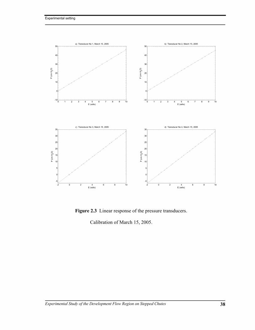
(Figure 2.3) were prepared and according with the tendency shown, a linear regression
between average voltage output (E) and water pressure (P) in centimeters was fit to the
data. Correlation coefficients larger than 0.999 were obtained in all calibrations.
2.4.2 Constant temperature anemometer
The anemometer was calibrated using a water tunnel with a jet submerging into a
reservoir in front of the jet (Figure 2.4). The water tunnel was made of Plexiglas and in it
the water was circulated through a rotameter into a stagnation section. At this section a
low-turbulence plug flow formed to enter the exit nozzle. The stagnation section was
made of a 33 cm piece of Plexiglas tube ( )7.5 cmφ = whilst the nozzle was a hose barb
to MIP adaptor ( )2.54 cm 0.64 cm× with an internal diameter of 4.72 mm. The
rotameter was a model GT-8-1306 with tube size R8M-127-4-F-BR-1/2-35G5, produced
by Brooks Instruments. This arrangement provided a range of velocities from 0.15 m/s to
5.40 m/s. The velocity was adjusted manually by means of a ball valve. Water was
supplied to the tunnel directly from the 60 cm supply pipeline through a clear hose
( )2.54 cmφ = attached at the available admission valve.
The nozzle water jet was calibrated using the volumetric method. In such a
procedure a graduate cylinder was used to record the volume of water, this cylinder had a
maximum capacity of 1000 ml and a graduation of 10 ml. Using this device and an
electronic stop watch, the 130 mm rotameter’ scale was calibrated against the indirect

Experimental setting
Experimental Study of the Development Flow Region on Stepped Chutes 29
velocity measurements. Once the rotameter was calibrated the water tunnel was ready to
be used with the constant temperature anemometer. To perform the static and dynamic
calibrations of the CTA system the procedure described in its instruction manual (DISA,
1977) was followed.
2.5 Modeling conditions
As mentioned before, the upstream boundary of the models was given by the
horizontal approach channel; therefore, the approaching fully rough flow defines an H2
profile in the vicinity of the stepped chute model (see Figure 2.5). The other upstream
boundary condition was given by the discharge; Table 2.2 indicates the range of
discharges for each flow regime according to the slope chute. On the other hand, the
downstream boundary condition was given by the fifth step; this brings the water from
the stepped chute to a rectangular channel ( )21.02 0.61 m× with a nearly horizontal slope
that conveyed the water to the recirculation tank. The flow in this channel did not affect
the hydraulic conditions in the chute models.
It is also opportune to mention the testing conditions in terms of the Reynolds
( )ER , Froude ( )Fr and Weber ( )We numbers. The Reynolds number during the tests
oscillated in the range of 63000 400000ER≤ ≤ while the Froude numbers varied from
2.5 5.8Fr≤ ≤ . The Weber numbers were in the range of 49 126We≤ ≤ . These values
were calculated at the downstream end of the first step. Appendix A indicates the flow
conditions for each one of the runs.

Experimental setting
Experimental Study of the Development Flow Region on Stepped Chutes 30
Table 2.2 Modeling conditions on the stepped chutes. Regime flow defined according to
Chanson and Toombes (2004). Discharge in 3m s .
Model slope
Regime 3.5 :1H V 5 :1H V 10 :1H V
Nappe flow 0.809cy h <
0.0545Q <
0.841cy h <
0.0578Q <
0.879cy h <
0.0618Q <
Transition flow 0.809 1.143cy h≤ ≤ 0.841 1.204cy h≤ ≤ 0.879 1.294cy h≤ ≤
Skimming flow 1.143cy h >
0.0916Q >
1.204cy h >
0.0991Q >
1.294cy h >
0.1103Q >
Finally, stepped chutes are usually built using step heights of 30, 60, 90 and 120
cm; being 60 and 90 cm the most common choice for RCC dams. The three models used
in the study had a step height of 15 cm and therefore they are related to prototype
conditions by scales of 1:2, 1:4, 1:6 and 1:8, respectively. Boes (2000) recommended
that a minimum scale of about 1:10 to 1:15 should be used in modeling stepped chutes in
order to minimize scale effects. Hence, the models used in this study are of sufficient
size to overcome the effects of viscous and surface tension forces introduce by the use of
the Froude similarity law.

Experimental setting
Experimental Study of the Development Flow Region on Stepped Chutes 31
2.6 Constant temperature anemometry
Constant temperature anemometry is based on the detection of the cooling effects
of fluid motion on a small heated sensor. The heat transfer is expressed by a particular
law that must be determined for each probe. In a non-isothermal water flow, this law is
significantly affected by the change in the physical properties of the water due to the
temperature drift as well as by the variation in overheat ratio due to the modification of
the temperature difference between the sensor and the water. Two procedures can be
used to minimize the influence of temperature drift: the constant overheat ratio and the
constant sensor temperature procedure.
The use of CTA in liquids is also affected by electrolysis, cracking of the sensor
quartz coating, presence of ions in the water, contamination and bubble formation on the
probe (Brunn, 1996). Electrolysis and cracking of the sensor quartz coating are strictly
related since the former is prevented by the latter. Cracking on the other hand, is usually
the result of a large potential drop between the water surrounding the probe and the film
element, this problem is resolved by connecting the CTA ground reference to the water.
The presence of ions is particularly important for multi-sensor probes where the
conductivity of the water can cause considerable cross-talk between sensors. The use of
de-ionized water and de-ionizer units is recommended to prevent ion effects. This type
of water is also recommended to prevent probe contamination in conjunction with the use
of bypass filtration units and algae inhibitors. Finally, the formation of bubbles on the
probe surface can be prevented by using a low overheat ratio. Rasmussen (1967)
concluded that the use of an overheat ratio smaller than 10% minimizes the possibility of
bubble formation.

Experimental setting
Experimental Study of the Development Flow Region on Stepped Chutes 32
2.6.1 Two-phase flow measurements using CTA
The development of instrumentation for two-phase flow is of the utmost
importance to back up theoretical investigations in many fields. Technically sound
measurement techniques provide information on the local structure of two-phase flows
characterized by the flow pattern, the specific area and the bubble diameter probability
function. Constant temperature anemometry has provided two-phase flow measurements
for more that 30 years; it exploits the large difference in heat transfer from the sensor to
the liquid and gas to discriminate the signal between the two phases. For a sufficient
long observation, the fraction of time the probe detects the gas can be interpreted as the
local void fraction.
In order to discriminate the hot-film signal into the gas and liquid phases, the
dynamic response of the anemometer output to the passage of a gas bubble across the
sensor needs to be well understood. As the bubble front approaches the probe the signal
output increases because the liquid in front of the bubble is moving with a greater
velocity than the average liquid velocity (Figure 2.6). The signal continues to increase
until the probe pierces the bubble (point A), and this is accompanied by a small overshoot.
The signal then shows a steep drop due to the evaporation of the liquid film on the sensor
surface. When the rear of the bubble arrives at the probe (point B), the rapid covering of
the probe with the liquid results in a steep rise in the signal output, this is the result of the
dynamic meniscus effect between the sensor and the liquid. This effect also produces an
overshot that is marked in Figure 2.2 as point C. The region immediately following this
point (up to point D) will also not represent a true continuous phase (Farrar et al., 1995).

Experimental setting
Experimental Study of the Development Flow Region on Stepped Chutes 33
Farrar and Bruun (1989) presented a complete description of the interaction between
bubbles and hot-film probes. Following the above description, for a continuous phase
evaluations the signal between A and D of each bubble must be eliminated. On the other
hand, the two events, A and B, correspond to the bubble front and the back contacting the
sensor, and need to be clearly identified to localize the bubble passage.
Several examples of bubble detection techniques can be found in the literature. In
general most of the techniques are variants of one (or combinations or both) of two basic
methods: the amplitude threshold method and the slope threshold method. In the
amplitude threshold method the raw anemometer signal is compared with a threshold
value. Any data points in the signal which lie below the voltage threshold are considered
to belong to the gas phase, and those points which are above the threshold voltage are
assumed to represent the continuous phase velocity. This method is easy to implement
and it is very effective in detecting a large proportion of the bubble in the signal.
However, some partial hits or very small bubbles may not be detected and more
important, it does not identify any of the important points A, B, C or D. On the other
hand, the slope threshold method uses the first derivative of the signal E t∂ ∂ and it
compares its value with one or more threshold levels. This method takes advantage of
the fact that the arrival of the front and rear of the bubble is associated with a sign change
in the time derivative of the signal. Similar criterion is used to detect the position of
points C and D.
Experimental setting
Experimental Study of the Development Flow Region on Stepped Chutes 34
2.6.2 Bubble detection method
The analysis of the CTA output signal requires the separation of the two flow
phases. In order to do so it is necessary to detect the bubbles by locating the points A, B,
C and D of each individual bubble. The detection technique employed in this study is
based on the methodology describe by Farrar et al. (1995). This methodology combines
the amplitude and the slope threshold methods and it takes into account the possibility of
water film breakage spike events. The amplitude threshold method is only used to detect
the presence of a bubble according to a preset threshold value while the slope threshold
method is used to determine the actual location of points A, B, C and D. The detection
method initiates by locating the point where the signal goes below the amplitude
threshold (Figure 2.7a), at this point it is considered that the sensor is in a bubble and a
two stage search is initiated. In the first stage the procedure looks backwards on the
signal and it compares the slope of the first derivative with a small negative slope
threshold to determine the location of point A (Figure 2.7b). Once point A is located, the
second stage looks forward for the point where the signal goes above the amplitude
threshold. At this point two new subroutines look for points B and C by comparing again
the first derivative of the signal with corresponding slope thresholds. Finally, a similar
procedure is used to locate point D. A more detail description of the methodology can be
found in Farrar et al. (1995).
2.6.3 Signal analysis
The CTA signal analysis initiates with the identification and consequent
separation of the continuous and gas phases, this is carried out using the technique

Experimental setting
Experimental Study of the Development Flow Region on Stepped Chutes 35
described in the previous section. Once the phases have been separated relevant
information can be obtained. In the continuous phase the signal output from the hot-film
anemometers is related to the local fluid velocity by the heat transfer law. From there,
the mean flow velocity (U ), the normal stress ( 2u ) and turbulence intensity ( )Tu can
easily be evaluated. These values are given by
1
1 k
jj
U un =
= ∑ , (2.1)
( )22
1
11
k
jj
u u Un =
= −− ∑ , (2.2)
and
2uTu
U= , (2.3)
where ju represent instantaneous water velocity values and k is the total number of
points on the liquid phase. In the case of the gas phase, the local void fraction (α ) is
defined as
ABtT
α = ∑ , (2.4)
where ABt is the time between points A and B (see Figure 2.6) and T is the total time of
the signal record (including both continuous and gas phase). Furthermore, the bubble
chord size is calculated as
ABs Ut= . (2.5)
Equation (2.2) assumes that the probe pierces through the center of each bubble, which
might not be always the case.

Experimental setting
Experimental Study of the Development Flow Region on Stepped Chutes 36
Figure 2.1 General layout of the models.

Experimental setting
Experimental Study of the Development Flow Region on Stepped Chutes 37
Figure 2.2 General overview of the models. a) Model I
during construction. b) Final layout of Model I. c)
Model I during initial tests. d) Overview of the
three models.
Experimental setting
Experimental Study of the Development Flow Region on Stepped Chutes 38
0 1 2 3 4 5 6 7 8 9 10-10
0
10
20
30
40
50
E (volts)
P (c
m H
2O)
a) Transducer No 1, March 15, 2005
0 1 2 3 4 5 6 7 8 9 10
-10
0
10
20
30
40
50
E (volts)
P (c
m H
2O)
b) Transducer No 2, March 15, 2005
-2 0 2 4 6 8 10
-5
0
5
10
15
20
25
30
35
E (volts)
P (c
m H
2O)
c) Transducer No 3, March 15, 2005
-2 0 2 4 6 8 10
-5
0
5
10
15
20
25
30
35
E (volts)
P (c
m H
2O)
d) Transducer No 4, March 15, 2005
Figure 2.3 Linear response of the pressure transducers.
Calibration of March 15, 2005.

Experimental setting
Experimental Study of the Development Flow Region on Stepped Chutes 39
Figure 2.4 Schematic diagram of the water tunnel.

Experimental setting
Experimental Study of the Development Flow Region on Stepped Chutes 40
-45 -40 -35 -30 -25 -20 -15 -10 -5 04
5
6
7
8
9
10
Wat
er d
epth
(cm
)
Remaining distance to step brink (cm)
25.0 l/s49.8 l/s
Figure 2.5 Measured H2 profiles on the approach channel.
0 1 2 3 4 5 6 7 81.6
1.7
1.8
1.9
2
2.1
2.2
2.3
Time (ms)
CTA
out
put v
olta
ge (
V )
↓A
← B
↓C
← D
Figure 2.6 Schematic representation of a signal from a
hot-film probe immersed in a liquid bubbly with gas
bubbles.

Experimental setting
Experimental Study of the Development Flow Region on Stepped Chutes 41
0 1 2 3 4 5 6 7 81.6
1.7
1.8
1.9
2
2.1
2.2
2.3
Time (ms)
CTA
out
put v
olta
ge (
V )
a)
↓A
← B
↓C
← D
Amplitude threshold↑
0 1 2 3 4 5 6 7 8-600
-400
-200
0
200
400
600
800
1000
1200
1400(b)
Time (ms)
Slo
pe (
V /
s)
Slope threshold↓
Figure 2.7 Schema of bubble detection method. a)
Amplitude threshold. b) slope threshold.

Constant temperature anemometry compensation
Experimental Study of the Development Flow Region of Stepped Chutes 42
Chapter 3 Constant temperature anemometry
compensation
3.1 Introduction
The procedures to compensate a constant temperature anemometer are described
in this chapter. Initially the two available procedures are introduced and later the
development of the heat transfer law is given. Finally, the effects of natural convection
are briefly discussed.
3.2 Temperature compensation
Temperature compensation is a procedure necessary when dealing with CTA
measurements in non-isothermal flows. Two procedures can be employed to compensate
for temperature drift: the constant sensor temperature and the constant overheat ratio
procedure.
Constant temperature anemometry compensation
Experimental Study of the Development Flow Region of Stepped Chutes 43
The two procedures differ significantly; the former requires several calibrations at
different water temperatures and operating resistances as well as constant monitoring of
the water temperature. The latter on the other hand, the constant overheat ratio procedure,
requires fewer calibrations (usually at the beginning and the end of the experiment) but
more frequent adjustments during the experimental runs.
3.3 Constant sensor temperature procedure
As the name suggests, in this procedure the temperature of the sensor is kept
constant and the anemometer output voltages are corrected before any heat transfer law is
sought. The sensor operating temperature ( )sT is kept constant by fixing the decade
resistance at the time of setup, and it remains unaltered during calibration and data
acquisition. In water flows, the expression of Morrow and Kline, cited by Stenhouse and
Stoy (1974), can be used to correct CTA output voltages. Morrow and Kline’s correction
is given by
S refref A
S A
T TE E
T T−
=−
, (3.1)
where refE and AE are the anemometer output voltages at a reference temperature refT
and water temperature AT ; Morrow and Kline used 22°C as the reference temperature.
Stenhouse and Stoy (1974) found Equation (3.1) to be quite accurate for water
temperatures ranging from 15°C to 28°C for the sensor temperature (44.5°C) that they
used during their tests. However, in the 16 tests carried out using the constant sensor
temperature procedure Equation (3.1) did not work adequately. In fact, a close inspection
of Figure 3.1 suggests that the temperature correction should depend on the flow velocity

Constant temperature anemometry compensation
Experimental Study of the Development Flow Region of Stepped Chutes 44
U since the calibration curves become closer to a logarithmic function as U decreases.
Figure 3.2 presents the variation of the Nusselt number Nu with overheat ratio Θ
expressed in terms of temperature as follows
S A
setup
T TT−
Θ = , (3.2)
where setupT is the water temperature at the time that the CTA system was setup. To
compute Nu , the physical properties of the water were evaluated at film temperature, i.e.,
the arithmetic average between ST and AT . Figure 3.2 indicates that for a given value of
flow velocity, a linear relationship between Nu and Θ exists. A result that is supported
by the fact that a linear relationship was also observed between the sensor cold resistance
oR and AT (see Figure 3.3). Once the linear dependence of Nu with Θ was established,
a heat transfer law or calibration curve for any other water temperature can be
interpolated in order to transform the CTA output voltages. Figure 3.4 compares the
results of using this approach with calibration test G13. As shown, values of flow
velocity agree within reasonable limits. Furthermore, an analysis of the ‘G’ tests indicate
that for a given CTA setup, calibration curves should be obtained within the expected
water temperature range in order to allow proper interpolation. However, the same tests
also suggest that if the water temperature varies more than 0.5 C° from its value at the
time of setup, the anemometer output signal deteriorates rapidly.
3.4 Constant overheat ratio procedure
In this procedure the overheat ratio is kept constant by manually or automatically
adjusting the anemometer resistance (Lekakis, 1996; Jørgensen, 2002). In doing so, the

Constant temperature anemometry compensation
Experimental Study of the Development Flow Region of Stepped Chutes 45
anemometer “sees” an isothermal flow since the excess temperature remains unaltered,
i.e., the difference between sensor operating temperature ST and the ambient (water)
temperature AT is unaltered. This procedure assumes that AT remains nearly constant
during each data acquisition. Figure 3.5 is a schematic representation of the manual
adjustment of overheat ratio. Initially, the variation of the sensor cold resistance ( )oR
with AT should be determined, subsequently, the sensor operating resistance ( )SR is
computed for the selected overheat ratio and the expected water temperature range. Next,
AT is measured and the value of the CTA decade resistance is adjusted to match the value
of SR at AT and the selected overheat ratio. Finally, the anemometer output voltage is
acquired.
As an example, Figure 3.6 presents two calibration curves of a conical hot-film
probe obtained by manually adjusting the decade resistance of the CTA system. The
difference between output voltages were smaller than 4% which speaks for the goodness
of the procedure. Automatic overheat adjustment would minimize temperature effects
even further.
3.4.1 Heat transfer law
To obtain the heat transfer law from curves like those in Figure 3.6 an analytical
calibration function relating E and U for a single sensor is needed. This calibration
function can take several forms. Wu and Bose (1993) suggested an extended power law
of the form

Constant temperature anemometry compensation
Experimental Study of the Development Flow Region of Stepped Chutes 46
2
0
kjn
jj
E A U=
= ∑ , (3.3)
where jA and n are experimental constants. King’s law is a specific case of Equation
(3.3) corresponding to 1k = ; the cases of 2k = and 3k = were also studied herein . It
has also been suggested (Bruun et al., 1988) the following variation of the extended
power law
20 1 2
nE A AU A U= + + . (3.4)
A third-order polynomial expression in terms of 2E has also been used (Bruun et
al., 1988; Lekakis, 1996) as well as a fourth-order polynomial in terms of E (Lekakis,
1996; Bruun, 1996; Jørgensen, 2002). Finally, Bruun et al. (1988) recommended the use
of cubic spline interpolation to fit the CTA raw data. The suitability of these functions to
accommodate the response of the conical hot-film probe was analyzed using Matlab™.
Values of the experimental constants and polynomial coefficients were obtained by the
least-squares fitting technique provided by Matlab™, the spline routine of this software
was also used in the analysis. To compare the goodness of fit the sum of squared error
was applied to the difference in flow velocite,i.e.,
( )2
1
N
m cj
U Uε=
= −∑ , (3.5)
where mU and cU are the measured and calculated flow velocity, respectively, and N is
the number of measured calibration values.
All the analytical functions, with the exception of 3k = in Equation (3.3),
followed the trend dictated by the cloud of ( ),E U points. Nevertheless, the spline, the
fourth order polynomial in terms of E , as well as the extended power law (Eq. (3.4))
Constant temperature anemometry compensation
Experimental Study of the Development Flow Region of Stepped Chutes 47
produce the smallest cumulative error (see Table 3.1). In fact, the cubic spline
interpolation produced a zero cumulative error, although this is not a surprising find since
the technique uses the provided ( ),E U values as knots. However, the spline
interpolation presented small wiggles which do not correspond to the probe response and
prevents a smooth fit through the velocity range. In addition, the spline interpolation did
not represent well the probe response at velocities smaller than 0.15 m/s (see Figure 3.7).
A similar problem was observed in the fourth order polynomial in terms of E , although it
did produce a smooth response over the velocity range. The extended power law
however, produced a good probe response while keeping a small error in the least-squares
fitting procedure. The downside of Equation (3.4) is there is no obvious solution for U ,
however, using Newton-Raphson its value can be obtained as
2
0 1 21 1
1 2
n
j j n
A AU A U EU UnAU A+ −
+ + −= −
+, (3.6)
which can be programmed in a few lines of code. Alternatively, a look-up table
technique will solve this inconvenience.

Constant temperature anemometry compensation
Experimental Study of the Development Flow Region of Stepped Chutes 48
Table 3.1 Sum of the squared error for the 12 tests.
Analytical function Cumulative ε
20 1
nE A AU= + 0.482
2 20 1 2
n nE A AU A U= + + 0.523
2 2 30 1 2 3
n n nE A AU A U A U= + + + 3309
20 1 2
nE A AU A U= + + 0.158
( ) ( ) ( )2 32 2 20 1 2 3U A A E A E A E= + + + 0.274
2 3 40 1 2 3 4U A A E A E A E A E= + + + + 0.150
Cubic spline interpolation 0
3.4.2 Sensitivity analysis
Since the overheat ratio was kept constant using a manual procedure, it was
necessary to estimate the effect of a possible overcompensation or an undercompensation
of the film probe. Figure 3.8 shows the effect of a unit variation of the decade resistance
on a calibration curve. As the figure indicates an overcompensation produces larger
voltages whilst an undercompensation produces smaller voltages for a given flow
velocity. Hence, overcompensation would produce larger velocity flows with the
possibility of extrapolation of the calibration curve whereas undercompensation would
produce smaller velocities. Table 3.2 presents the error in output voltage as well as in
flow velocity estimation due to an over or an under compensation. As the table shows,

Constant temperature anemometry compensation
Experimental Study of the Development Flow Region of Stepped Chutes 49
both conditions produce significant error and therefore compensation is a critical issue
when it is carried out manually.
Table 3.2 Variation of the CTA output voltage with a unit
change in decade resistance.
Error in E Error in U
U
(m/s)
Minus one
(%)
Plus one
(%)
Minus one
(%)
Plus one
(%)
0 -4.3 3.0 0 0
0.19 -6.2 4.6 -49 132
0.59 -6.4 5.5 -62 69
0.94 -6.5 5.8 -53 89
2.42 -6.9 6.6 -49 90
3.9 -7.1 6.9 -50 -550
5.5 -7.5 7.0 -51 -609
3.5 Buoyancy effects
Buoyancy effects occur at low velocities when convection currents form because
of the buoyancy of the heated fluid surrounding the sensor. Thus, the sensor losses heat
by convection even in still air and this free convection flow tends to mask any low-
velocity forced convection cooling. Collins and Williams (1959) concluded that
buoyancy effects are small provided
1 3ER Gr= , (3.7)

Constant temperature anemometry compensation
Experimental Study of the Development Flow Region of Stepped Chutes 50
where ER and Gr are the Reynolds and Grashof numbers, respectively. Dantec
Dynamics (2003) indicates that natural convection overrules the forced convection when
ER is smaller than twice 1 3Gr , i.e., a safety factor of two in Equation (3.7). Figure 3.9
presents the case of a typical conical hot-film probe operated at a constant overheat ratio
of 10% in a water flow. As shown in the figure, the probe would safely operate in the
forced convection zone at water flow velocities as low as 0.5 cm/s. Dantec Dynamics
(2005) indicates that conical probes have influence from natural convection up to
approximately 0.1 m/s in air flows, no indication is given for water flows.
3.6 Final comments
It has been found that the three problems attributed to the use of CTA in water
flows measurements can be overcome by an appropriate selection of the overheat ratio
and a careful use of the proper temperature compensation technique.
Temperature drift may be compensated adequately by using the constant sensor
temperature procedure as long as the water temperature variations are smaller than 0.5 C° .
The compensation is performed by applying a temperature correction to the raw data.
This correction not only depends on the overheat ratio but also on the flow velocity. In
the present case, a linear correction in terms of the Nusselt number and the actual
overheat ratio Θ was obtained for each fixed value of flow velocity. In addition, heat
transfer laws for the expected water temperature range should be obtained for each CTA
setup condition, i.e., for each fixed value of sR .
Constant temperature anemometry compensation
Experimental Study of the Development Flow Region of Stepped Chutes 51
On the other hand, compensation of temperature drift by means of the constant
overheat ratio procedure produces good results and does not require numerous
calibrations. Hence, in water flows this procedure should be preferred over the constant
sensor temperature one. In the present study, manual compensation produced good
results and minimized the effects of temperature change and, it is expected that a fully
automatic process would produce even better results. From the analytical functions
tested, the use of an extend power law in form of Equation (3.4) produced a good and
smooth representation of the conical hot-film probe response. A fourth order polynomial
in terms of E does produce satisfactory results although there is the risk of strong
deviations in the lower range of flow velocities. Cubic spline interpolation also has this
weakness with the additional presence of small wiggles. The use of a larger number of
calibration points may enhance the performance of these two analytical functions.
Finally, probe contamination, can be easily overcome by performing frequent
calibrations. In addition, the conical hot-film probe employed herein was used for more
than 300 hours with no appreciable contamination effects, this is in spite of the fact that
no special measurements were taken to prevent such effects; these results are encouraging
when considering the use of the hot-film anemometry technique in experimental
procedures where large water flows are involved. Furthermore, buoyancy effects are
likely to occur only at extremely low velocities, which where not present in these data.

Constant temperature anemometry compensation
Experimental Study of the Development Flow Region of Stepped Chutes 52
0 1 2 3 4 5 6
0.8
1
1.2
1.4
1.6
1.8
2
2.2
2.4
2.6
U (m/s)
E (
volts
)
Run G1, 17.4 oC
Run G2, 19.0 oC
Run G3, 19.3 oC
Run G4, 19.4 oC
Figure 3.1 Calibration curves of a conical probe using the
constant sensor temperature procedure. Overheat
ratio = 10% , 18.5setupT C= ° , 15.53SR = ohms.
1.48 1.5 1.52 1.54 1.56 1.58 1.6 1.62 1.6410
20
30
40
50
60
70
80
90
100
Θ
Nu
U = 0 m/sU = 0.59 m/sU = 2.42 m/sU = 5.45 m/s
Figure 3.2 Variation of Nu with actual overheat ratio Θ .
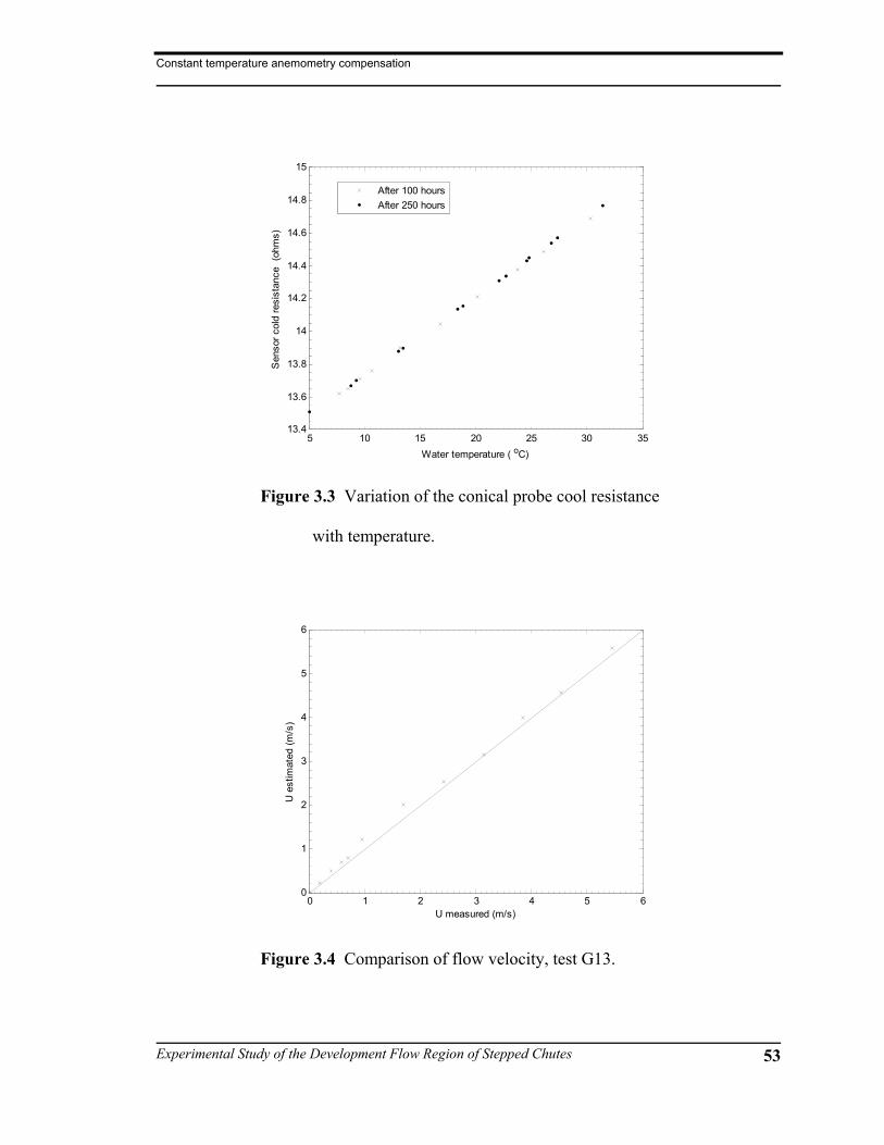
Constant temperature anemometry compensation
Experimental Study of the Development Flow Region of Stepped Chutes 53
5 10 15 20 25 30 3513.4
13.6
13.8
14
14.2
14.4
14.6
14.8
15
Water temperature ( oC)
Sen
sor c
old
resi
stan
ce (
ohm
s)
After 100 hoursAfter 250 hours
Figure 3.3 Variation of the conical probe cool resistance
with temperature.
0 1 2 3 4 5 60
1
2
3
4
5
6
U measured (m/s)
U e
stim
ated
(m/s
)
Figure 3.4 Comparison of flow velocity, test G13.

Constant temperature anemometry compensation
Experimental Study of the Development Flow Region of Stepped Chutes 54
Figure 3.5 Schematic diagram of the manual adjustment of
the overheat ratio.
0 1 2 3 4 5 61
1.2
1.4
1.6
1.8
2
2.2
2.4
U (m/s)
E (v
olts
)
test H3, 23.6 oC
test H4, 25.2 oC
Figure 3.6 Example of test results using the constant
overheat ratio technique.
Obtain Ro = Ro ( TA )
Read TA
Adjust CTA decade resistance to match RS
at TA
Acquire CTA output
voltage Continue
start
end
yes no
Compute RS for TA range and
overheat ratio

Constant temperature anemometry compensation
Experimental Study of the Development Flow Region of Stepped Chutes 55
-1 0 1 2 3 4 5 61
1.2
1.4
1.6
1.8
2
2.2
2.4
U (m/s)
E (v
olts
)
Test H7Equation [3.4]
4th order polynomial in ECubic spline interpolation
Figure 3.7 Fitting results of analytical functions, test H7.
0 1 2 3 4 5 61
1.2
1.4
1.6
1.8
2
2.2
2.4
U (m/s)
E (
volts
)
Calibration dataMinus onePlus one
Figure 3.8 Variation of the CTA output with changes in
decade resistance.

Constant temperature anemometry compensation
Experimental Study of the Development Flow Region of Stepped Chutes 56
5 10 15 20 25 30
0.2
0.25
0.3
0.35
0.4
0.45
0.5
Water temperature ( oC)
U (c
m/s
)
Forced convection
Free convection
Figure 3.9 Region of forced and free convection flow for a
typical conical hot-film probe operated with the
constant overheat ratio technique. Overheat ratio
set at 10%.
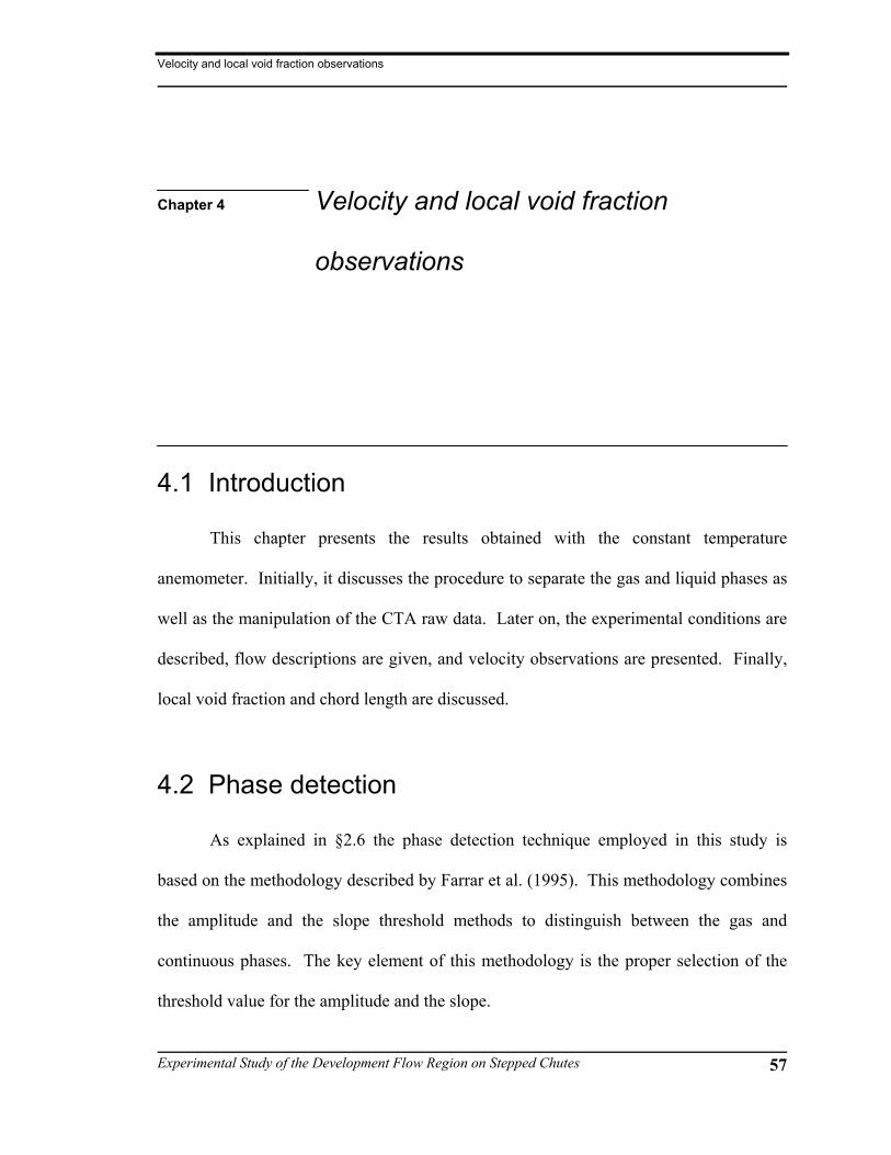
Velocity and local void fraction observations
Experimental Study of the Development Flow Region on Stepped Chutes 57
Chapter 4 Velocity and local void fraction
observations
4.1 Introduction
This chapter presents the results obtained with the constant temperature
anemometer. Initially, it discusses the procedure to separate the gas and liquid phases as
well as the manipulation of the CTA raw data. Later on, the experimental conditions are
described, flow descriptions are given, and velocity observations are presented. Finally,
local void fraction and chord length are discussed.
4.2 Phase detection
As explained in §2.6 the phase detection technique employed in this study is
based on the methodology described by Farrar et al. (1995). This methodology combines
the amplitude and the slope threshold methods to distinguish between the gas and
continuous phases. The key element of this methodology is the proper selection of the
threshold value for the amplitude and the slope.

Velocity and local void fraction observations
Experimental Study of the Development Flow Region on Stepped Chutes 58
Delhaye (1968) pointed out that the probability density function corresponding to
a very large sample of hot-film data have a bimodal shape (See Figure 4.1a), consisting
of two peaks separated by a lower level plateau region. In a bubbly two-phase flow the
modal peak at large voltages corresponds to the fluctuations associated with the
continuous phase turbulence whilst the other modal peak reflects the bubble passage, this
is located on the range of low voltage values of the hot-film signal.
Several approaches were attempted to separate the two phases. Initially, the hot-
film signal was considered a mixture of two normal distributions, one for each phase.
Under this assumption a maximum likelihood estimation algorithm (Agna and Ibrahim,
1984) was employed to determine the statistical parameters (mean and standard
deviation) of the two individual distributions. Using these parameters, the amplitude
threshold value was selected from the voltage/velocity Gaussian distribution as the value
with probability of occurrence of 5%. However, inspection of the sample histogram
indicated that the voltage/velocity sub-sample tends to be negatively skew and therefore
the sub-sample mean value was smaller than the mode value. Hence, the computed
threshold value was often too small and inside the gas phase, especially if the spread of
the continuous phase was large. As a consequence of this small threshold value the
parameters of both phases were computed incorrectly.
Another approach consisted in dividing the anemometer signal into two sub-
samples using the average between the two extreme values of the signal record. Then,
the continuous phase sub-sample was checked for normality using Lilliefors’ test
(Lilliefors, 1967) and, if the Gaussian distribution was confirmed, the standard deviation
was calculated, otherwise, the standard deviation was assumed to be equal to the

Velocity and local void fraction observations
Experimental Study of the Development Flow Region on Stepped Chutes 59
interquartile range (IQR). Finally, using these two parameters the threshold value was
selected as the mode minus twice the standard deviation. This would correspond
approximately to a probability of 5% in a normal distribution. This procedure corrected
the location since it explicitly uses the mode but once again, the obtained threshold
values were small due to the large spread of some samples. So, a new approach was
sought.
The new approach consisted of taking a sub-sample of the signal values larger
than a prefix voltage in the plateau region of probability density function. Then, the
mode of the sub-sample was obtained and the empirical cumulative density function
between the minimum value and the mode was calculated. Finally the autocorrelation
values of the empirical cumulative density function were calculated and the threshold
value was selected at the point were the autocorrelation was zero (see Figure 4.1b). The
selection of this point is based on the idea that if the CTA output voltage is in the plateau
region the relative frequency of each bin shown in Figure 4.1a is similar, hence, the
increments of the empirical cumulative density function are nearly constant and so the
autocorrelation is close to one. As the voltage gets into the continuous phase, the relative
frequencies become larger and the increments on the cumulative density function do so as
well; at this moment the autocorrelation begins to decrease and it goes to zero where the
increment given by the relative frequency is completely dissimilar (or independent) from
the previous one.
The above approaches were also used to select the threshold value for the slope
method. Nevertheless, close inspection of the time series of CTA output voltages (Fig.
4.2a) and its corresponding slope plots (Fig. 4.2b) suggested that the proper selection of

Velocity and local void fraction observations
Experimental Study of the Development Flow Region on Stepped Chutes 60
the bubble characteristic points were obtained by setting the threshold value at zero, i.e.,
when the slope signal changes its sign.
4.3 Voltage correction
The possibility of inducing errors by overcompensation or under-compensation
was introduced in §3.4. Therefore, it was necessary to develop a procedure to correct this
issue; this was done using the information of the sensitivity analysis presented in the
previous chapter. Figure 4.3a presents the relationships between the corrected CTA
output voltages and an overcompensated or undercompensated signal. The relationships
are linear, which simplified greatly the analysis. Figure 4.3b presents of am example of a
velocity profile with an error induced by overcompensation. As seen in the figure, the
top 3 points show a step in velocity and are clearly different from the trend. Inspection of
the water temperature and CTA decade resistance records indicated that different settings
were used for these three points than for the previous eight, i.e., at point 9th the decade
resistance was manually readjusted. Using the linear relationships from Figure 4.3a, the
raw voltage values of the time series for these three points were corrected and the correct
velocity profile was obtained. This procedure was followed in all cases that present an
error by over/under compensation.
4.4 Experimental conditions
As mentioned in §2.3 a constant temperature anemometer equipped with a conical
hot-film probe was used to record the flow velocities. Data acquisition was carried out at
Velocity and local void fraction observations
Experimental Study of the Development Flow Region on Stepped Chutes 61
a frequency of 5000 Hz for 180 second duration. The precision of the data acquisition
card was set to 1.22± mV and the water temperature was collected manually using a
digital platinum resistance thermometer (Guildline, model 9540) with a resolution of
0.01 C° . Measurements were obtained in the width centerline and vertical positioning
was manually controlled using a point gauge with a precision of 0.02± cm.
Measurements on Model I ( )3.5 :1H V were carried out using the constant sensor
temperature procedure discussed in §3.3. This procedure is quite sensitive to water
temperature fluctuations and unfortunately, temperature drift compromised the quality of
the time series. Hence, it was decided not to include the CTA data of Model I in this
study. On the other hand, measurements on Models II and III (5 :1H V and 10 :1H V ,
respectively) were taken using the constant overheat ratio procedure presented in §3.4.
4.5 Flow description
The flow conditions on the models varied greatly. The effect of providing air into the
step cavity only had effects on nappe flow regime and they were limited to the first step.
Figure 4.4 and 4.5 shows the first two steps of Models II and III, respectively. As seen in
these figures provision of air on the first step did have an effect on the flow geometry. If
air was provided into the step cavity the formation of the air pocket was possible (Figures
4.4a and 4.5a) and the flow resembled a drop structure. Nevertheless if air was not
provided, the jet was depleted towards the step riser (see Figures 4.4b and 4.5b), there
was no air pocket and the jet struck at a stepper angle. In either case however, no flow
disturbance was observed downstream of the jet impact and clear water prevailed along
the step. On the contrary, whether air was provided or not into the step cavity of the

Velocity and local void fraction observations
Experimental Study of the Development Flow Region on Stepped Chutes 62
second step did not produced appreciable difference on the flow geometry (see Figures
4.4c-d and 4.5c-d). Furthermore, air was observed in the jet and inside the recirculating
pool while significant flow disturbance was observed at the jet impact. It is also worth
mentioning that supercritical flow was always observed along the steps during all the
tests carried out.
On nappe flow regime the flow characteristics change in downstream direction.
As mentioned before, the geometry on the first step depends on whether air was provided
or not into the step cavity. On Models II and III the jet remain supercritical along this
step and no air was observed in the main stream although small bubbles were observed at
the interface between the jet and the air pocket (see Figures 4.6a and 4.7a). On the
second step, the air pocket was always observed suggesting that the jet was sufficiently
broken at this drop to allow air into the cavity. The recirculating pools still resembled the
one from a drop structure. At the jet impact, there was considerable turbulence as well as
air entrainment (Figures 4.6b and 4.7b). From this point onwards Models II and III
behaved differently. On Model II, the flow adopted a white water condition due to the
presence of air and flow disturbances were carried in downstream direction; the
proximity of next drop did not give enough length to the jet to reorganize and become
once again a coherent jet. Hence, the jet became more turbulent as the flow moved in
downstream direction. On the contrary, on Model III the length of the step tread provides
sufficient space for the flow to dissipate the disturbances, release the air bubbles and act
as a single jet once again at the next drop. The third step on model II was characterized
by a complete two phase flow situation and disintegration of the jet (Figure 4.6c). The
recirculating pool was shallow and elongate with significant oscillation of the water

Velocity and local void fraction observations
Experimental Study of the Development Flow Region on Stepped Chutes 63
surface. On Model III, more air entrainment and turbulence was observed at the jet
impact than at the previous step (Figure 4.7c), the subsequent turbulence dissipation and
air release took also longer than at step 2. Nevertheless close to the brink, the flow
showed some bubbles but the flow was generally calm. As in the case of Model II, the
recirculating pool was shallow and elongate when compared to the drop structure.
Finally, at step 4 the flow on model II was more chaotic than in the previous step with a
jet completely disintegrated in a two phase flow situation (Figure 4.6d). In Model III, the
flow is similar than in the previous step but more air bubbles were observed close to the
brink (Figure 4.7d).
Figure 4.8 and 4.9 show the transition flow regime. Model II (Figure 4.8)
presented a clear water flow on step 1 with the water surface in phase with the step
geometry. Nevertheless, the water surface had little oscillations; the step cavity was full
of water with no air bubbles and a vortex formed inside it. On step 2 the jet began to
entrain air, bubbles were observed inside the recirculating pool and along the jet. Within
the recirculating pool, the bubbles concentrated towards the jet. Downstream of the jet
impact the jet began to break and significant amount of splash developed. Notably, this
regime presented significant amount of spray; drops were detected to reach 4 to 5h
above the chute invert on average, although, some drops were observed at 7 to 8h . On
step 3 significant amount of air was observed as well as a small air pocket. The flow was
a mixture of air and water and the jet was completely broken. At step 4, the air pocket
was bigger with large oscillations on the water surface of the recirculating pool. On
Model III (Figure 4.9), the first step also had clear water with no air cavity or air bubbles.
As in Model II, little oscillations on the water surface were also observed but the water

Velocity and local void fraction observations
Experimental Study of the Development Flow Region on Stepped Chutes 64
surface remained in phase with the step geometry. On step 2, the jet began to disintegrate
after hitting the tread and most of the air entrainment occurred at this point. The step
cavity was full of water although a small air pocket randomly formed. Figure 4.10
depicts the formation of air pocket. Initially, the step cavity had little bubbles along the
boundary between the jet and the recirculating pool (Figure 4.10a). The subsequent
photos (Figures 4.10b-c) show the entrainment of air at this boundary which will
eventually produce a small air pocket (not shown) and then, the air was carried away
(Figures 4.10d-e) leaving the step cavity in a clear water conditions. Downstream of the
jet impact the water surface was irregular and the flow carried pocket of bubble, probably
released from the step cavity. Moreover, step 3 also presented the random formation of
the air cavity, the flow carried significant amount of air and the jet was clearly broken
and marked by considerable deformation of the water surface. At the step 4, there was a
permanent air cavity, the flow was a air-water mixture and highly fragmentated.
The skimming flow regime on model II presented a water surface in phase with
the step geometry, clear water flow and step cavities completely filled with water (see
Figure 4.11). On the third step some bubbles were observed inside the recirculating pool
while at step 4 bubbles were also observed in the jet. Small oscillations of the water
surface were also observed in steps 3 and 4, which gave a white water appearance when
looking from the top. Vortices were presented inside the step cavities. Model III also
presented a clear water flow in phase with the chute geometry in the first two steps
(Figure 4.12). Beyond this step surface oscillation became important and a three
dimensional feature began to develop. This feature corresponded to shock waves which
can be observed in Figure 4.13. Model II did also present such feature but the breaking

Velocity and local void fraction observations
Experimental Study of the Development Flow Region on Stepped Chutes 65
process of the jet masked these waves and prevented its development. As the flow
progressed downstream on Model III, the shock waves became bigger and they brought
air into the upper part of the flow as seen in Figures 4.12c and 4.12d. Furthermore, inside
the step cavity of steps 3 and 4, that is, the steps affected by shock waves, a three-
dimensional ascendant spiral flow was observed in the zone close to the step riser. This
flow was directed towards the step riser on the bottom part and then towards the sides of
the chute with an upward direction that gave the spiral movement. The formation of
these spiral vortices is probably due to the action of the shock waves.
4.6 Velocity observations
Measured velocity profiles at the step brinks are presented in Figures 4.14 to 4.19.
Appendices B and C give profiles at other locations for Models II and III, respectively.
Profiles of velocity gradient, turbulence intensity and normal stress are also given in
those appendices. For these profiles the water depth ( )y was measured with respect to
the step tread and Ty is the total water depth. The velocity is represented by U , and
avgU corresponds to the depth flow average velocity.
Figures 4.14 and 4.15 present the nappe flow velocity profiles on Models II and
III, respectively. As the figures show, there is no appreciable difference between the
aerated and non-aerated condition. The profiles on step 1 present a logarithmic
distribution as in open channel flow, which progressively disappears as the water moves
downstream, especially at large discharges as in Figure 4.15. Between models, the

Velocity and local void fraction observations
Experimental Study of the Development Flow Region on Stepped Chutes 66
velocity profiles at the brinks are similar (Figure 4.16 and 4.17) before the jets break up,
once this occurs, there is no defined velocity distribution as the flow losses its coherence.
Figures 4.18 and 4.19 present the velocity profiles for transition and skimming
flow. There is general agreement between models and the profile follow a logarithmic
distribution on those steps with clear water.
4.7 Local void fraction observations
It is well known that air bubbles not only modify the flow characteristics but also
the downstream water quality. Specifically, high levels of turbulence and large air-water
interface area enhance the transfer of atmospheric and volatile gases between air and
water. Knowledge about the variables involve in this transfer mechanism is
indispensable in the design of water treatment systems and preservation of aquatic habitat,
since it is often observed saturation of dissolved oxygen and nitrogen downstream of
hydraulic structures carrying air-water flows. In this regard, turbulence levels were
already presented in the previous section while quantification of the interface area
requires the knowledge of three basic parameters: local void fraction, bubble count rate
and bubble chord length.
Local void fractions at the step brinks are presented in Figures 4.20 to 4.25.
Several other locations are given in Appendices B and C. According to the observations,
specifically, the local void fraction is not affected by the conditions of the step cavity,
Figures 4.20 and 4.21 indicated that similar results were recorded for an aerated and non-
aerated step cavity. Furthermore, similar results were also obtained between models.
The air concentration seems to have a “C” shape, that is, larger values were observed at

Velocity and local void fraction observations
Experimental Study of the Development Flow Region on Stepped Chutes 67
the bottom and top while minimum values in the middle of the water column. The
observations also indicate that air concentration in the development flow region remains
below 0.6.
The chord length of a bubble is the length of the straight line connecting the two
points where the tip of the conical probe pierces the bubble whilst bubble count rate is the
number of bubble impacting the probe tip. Chord length distributions as well as bubble
count rates are shown in Appendices B and C. The results indicate that within a step,
larger chord lengths are obtained along the step tread than at the brink, specifically,
immediately after the sliding jet hits the step tread. Furthermore, the trend of the chord
length is to increase in downstream direction (from brink to brink) and results indicated
that it stays smaller than about 12 mm. At the step brink, larger chord sizes were
recorded on Model II than on Model III, likely due to the fact that the tread on the former
is halve the size of the latter giving time for large bubbles to reach the surface.

Velocity and local void fraction observations
Experimental Study of the Development Flow Region on Stepped Chutes 68
0.8 1 1.2 1.4 1.6 1.8 2 2.20
0.01
0.02
0.03
0.04
0.05
0.06(a)
CTA output voltage (Volts)
Rel
ativ
e fre
quen
cy
1.7 1.75 1.8 1.85 1.9 1.95 2-0.5
0
0.5
1
CTA output voltage (Volts)
Aut
ocor
rela
tion
(b)
Figure 4.1 Selection of voltage threshold. a) histogram of
CTA output voltage b) autocorrelation plot.
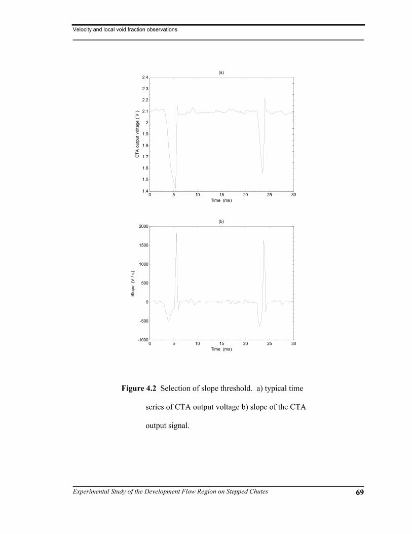
Velocity and local void fraction observations
Experimental Study of the Development Flow Region on Stepped Chutes 69
0 5 10 15 20 25 301.4
1.5
1.6
1.7
1.8
1.9
2
2.1
2.2
2.3
2.4(a)
Time (ms)
CTA
out
put v
olta
ge (
V )
0 5 10 15 20 25 30-1000
-500
0
500
1000
1500
2000(b)
Time (ms)
Slo
pe (
V /
s)
Figure 4.2 Selection of slope threshold. a) typical time
series of CTA output voltage b) slope of the CTA
output signal.

Velocity and local void fraction observations
Experimental Study of the Development Flow Region on Stepped Chutes 70
1 1.2 1.4 1.6 1.8 2 2.2 2.41
1.2
1.4
1.6
1.8
2
2.2
2.4(a)
Measured voltage (volts)
Cor
rect
ed v
olta
ge (
volts
)
Minus onePlus one
0 0.2 0.4 0.6 0.8 1 1.2 1.4 1.6 1.8 20
0.1
0.2
0.3
0.4
0.5
0.6
0.7
0.8
0.9
1
U / Uavg
y / y
T
(b)
BeforeAfter
Figure 4.3 Correction of voltages. a) relationship between
corrected voltage and under-compensated (minus
one) and over-compensate signal (plus one) b)
velocity profile before and after correction.

Velocity and local void fraction observations
Experimental Study of the Development Flow Region on Stepped Chutes 71
a) b)
c) d)
Figure 4.4 Step cavity conditions on Model II. a) step 1,
aerated. b) step 1, non-aerated. c) step 2, aerated. d)
step 2, non-aerated.

Velocity and local void fraction observations
Experimental Study of the Development Flow Region on Stepped Chutes 72
a) b)
c) d)
Figure 4.5 Step cavity conditions on Model III. a) step 1,
aerated. b) step 1, non-aerated. c) step 2, aerated. d)
step 2, non-aerated.

Velocity and local void fraction observations
Experimental Study of the Development Flow Region on Stepped Chutes 73
a) b)
c) d)
Figure 4.6 Nappe flow regime on Model II. Non-aerated
step cavity, 0.51cy h = . a) step 1. b) step 2. c) step
3. d) step 4.
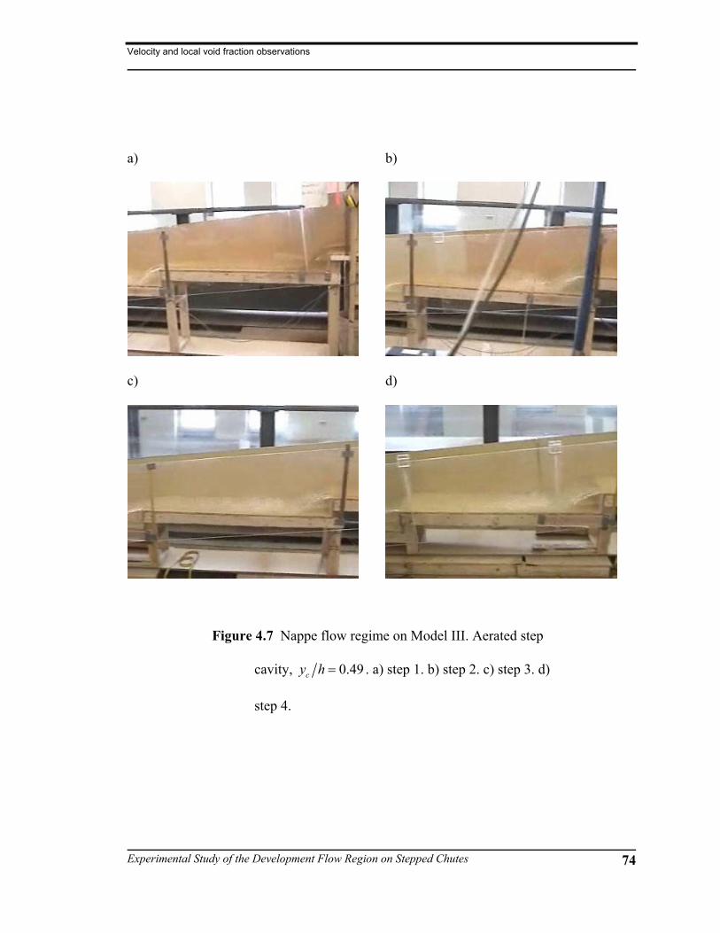
Velocity and local void fraction observations
Experimental Study of the Development Flow Region on Stepped Chutes 74
a) b)
c) d)
Figure 4.7 Nappe flow regime on Model III. Aerated step
cavity, 0.49cy h = . a) step 1. b) step 2. c) step 3. d)
step 4.

Velocity and local void fraction observations
Experimental Study of the Development Flow Region on Stepped Chutes 75
a) b)
c) d)
Figure 4.8 Transition flow regime on Model II. Non-
aerated step cavity, 1.01cy h = . a) step 1. b) step 2.
c) step 3. d) step 4.

Velocity and local void fraction observations
Experimental Study of the Development Flow Region on Stepped Chutes 76
a) b)
c) d)
Figure 4.9 Transition flow regime on Model III. Aerated
step cavity, 1.09cy h = . a) step 1. b) step 2. c) step
3. d) step 4.

Velocity and local void fraction observations
Experimental Study of the Development Flow Region on Stepped Chutes 77
a) b)
c) d)
e)
Figure 4.10 Entrainment of air into the step cavity. Model
III, 1.09cy h = , step 2. Imagines approximately
every 0.4 s.

Velocity and local void fraction observations
Experimental Study of the Development Flow Region on Stepped Chutes 78
a) b)
c) d)
Figure 4.11 Skimming flow regime on Model II. Non-
aerated step cavity, 1.66cy h = . a) step 1. b) step 2.
c) step 3. d) step 4.

Velocity and local void fraction observations
Experimental Study of the Development Flow Region on Stepped Chutes 79
a) b)
c) d)
Figure 4.12 Skimming flow regime on Model III. Aerated
step cavity, 1.66cy h = . a) step 1. b) step 2. c) step
3. d) step 4.

Velocity and local void fraction observations
Experimental Study of the Development Flow Region on Stepped Chutes 80
a)
b)
Figure 4.13 Shock waves at skimming flow regime. a)
Model II. b) Model III.
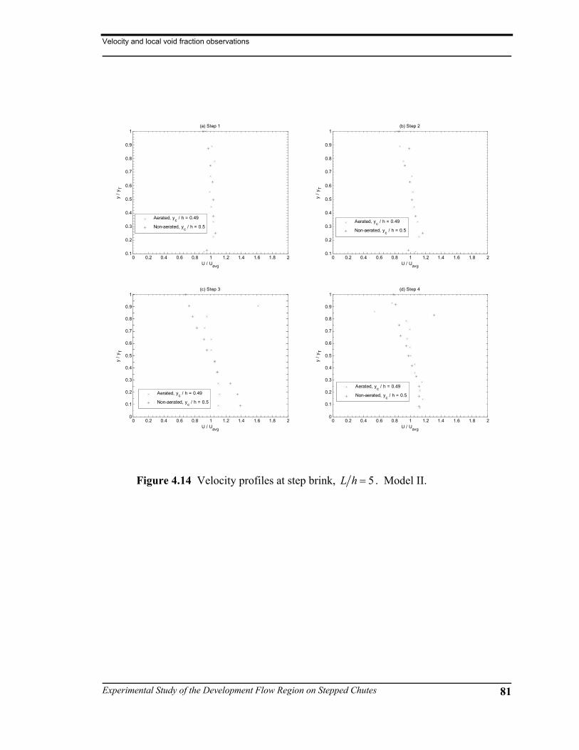
Velocity and local void fraction observations
Experimental Study of the Development Flow Region on Stepped Chutes 81
0 0.2 0.4 0.6 0.8 1 1.2 1.4 1.6 1.8 20.1
0.2
0.3
0.4
0.5
0.6
0.7
0.8
0.9
1(a) Step 1
y / y
T
U / Uavg
Aerated, yc / h = 0.49
Non-aerated, yc / h = 0.5
0 0.2 0.4 0.6 0.8 1 1.2 1.4 1.6 1.8 20.1
0.2
0.3
0.4
0.5
0.6
0.7
0.8
0.9
1(b) Step 2
y / y
T
U / Uavg
Aerated, yc / h = 0.49
Non-aerated, yc / h = 0.5
0 0.2 0.4 0.6 0.8 1 1.2 1.4 1.6 1.8 20
0.1
0.2
0.3
0.4
0.5
0.6
0.7
0.8
0.9
1(c) Step 3
y / y
T
U / Uavg
Aerated, yc / h = 0.49
Non-aerated, yc / h = 0.5
0 0.2 0.4 0.6 0.8 1 1.2 1.4 1.6 1.8 20
0.1
0.2
0.3
0.4
0.5
0.6
0.7
0.8
0.9
1(d) Step 4
y / y
T
U / Uavg
Aerated, yc / h = 0.49
Non-aerated, yc / h = 0.5
Figure 4.14 Velocity profiles at step brink, 5L h = . Model II.

Velocity and local void fraction observations
Experimental Study of the Development Flow Region on Stepped Chutes 82
0 0.2 0.4 0.6 0.8 1 1.2 1.4 1.60
0.1
0.2
0.3
0.4
0.5
0.6
0.7
0.8
0.9
1(a) Step 1
y / y
T
U / Uavg
Aerated, yc / h = 0.8
Non-aerated, yc / h = 0.77
0 0.2 0.4 0.6 0.8 1 1.2 1.4 1.60
0.1
0.2
0.3
0.4
0.5
0.6
0.7
0.8
0.9
1(b) Step 2
y / y
T
U / Uavg
Aerated, yc / h = 0.8
Non-aerated, yc / h = 0.77
0 0.2 0.4 0.6 0.8 1 1.2 1.4 1.60
0.1
0.2
0.3
0.4
0.5
0.6
0.7
0.8
0.9
1(c) Step 3
y / y
T
U / Uavg
Aerated, yc / h = 0.8
Non-aerated, yc / h = 0.77
0 0.2 0.4 0.6 0.8 1 1.2 1.4 1.60
0.1
0.2
0.3
0.4
0.5
0.6
0.7
0.8
0.9
1(d) Step 4
y / y
T
U / Uavg
Aerated, yc / h = 0.8
Non-aerated, yc / h = 0.77
Figure 4.15 Velocity profiles at step brink, 10L h = . Model III.

Velocity and local void fraction observations
Experimental Study of the Development Flow Region on Stepped Chutes 83
0 0.2 0.4 0.6 0.8 1 1.2 1.4 1.60
0.1
0.2
0.3
0.4
0.5
0.6
0.7
0.8
0.9
1(a) Step 1
y / y
T
U / Uavg
Model II, yc / h = 0.78
Model III, yc / h = 0.8
0 0.2 0.4 0.6 0.8 1 1.2 1.4 1.60
0.1
0.2
0.3
0.4
0.5
0.6
0.7
0.8
0.9
1(b) Step 2
y / y
T
U / Uavg
Model II, yc / h = 0.78
Model III, yc / h = 0.8
0 0.2 0.4 0.6 0.8 1 1.2 1.4 1.60
0.1
0.2
0.3
0.4
0.5
0.6
0.7
0.8
0.9
1(c) Step 3
y / y
T
U / Uavg
Model II, yc / h = 0.78
Model III, yc / h = 0.8
0 0.2 0.4 0.6 0.8 1 1.2 1.4 1.60
0.1
0.2
0.3
0.4
0.5
0.6
0.7
0.8
0.9
1(d) Step 4
y / y
T
U / Uavg
Model II, yc / h = 0.78
Model III, yc / h = 0.8
Figure 4.16 Comparison of velocity profiles with aerated flows at step
brinks. Model II at 5L h = , Model III at 10L h = .
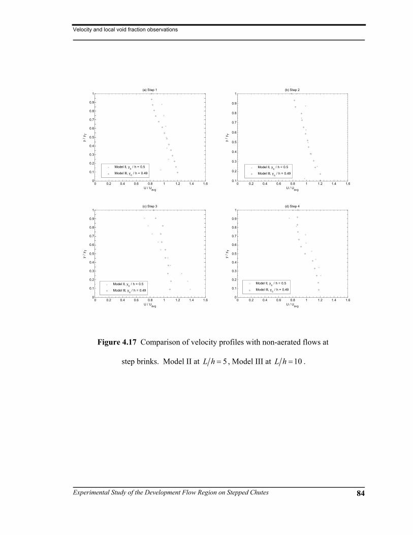
Velocity and local void fraction observations
Experimental Study of the Development Flow Region on Stepped Chutes 84
0 0.2 0.4 0.6 0.8 1 1.2 1.4 1.60
0.1
0.2
0.3
0.4
0.5
0.6
0.7
0.8
0.9
1(a) Step 1
y / y
T
U / Uavg
Model II, yc / h = 0.5
Model III, yc / h = 0.49
0 0.2 0.4 0.6 0.8 1 1.2 1.4 1.60.1
0.2
0.3
0.4
0.5
0.6
0.7
0.8
0.9
1(b) Step 2
y / y
T
U / Uavg
Model II, yc / h = 0.5
Model III, yc / h = 0.49
0 0.2 0.4 0.6 0.8 1 1.2 1.4 1.60
0.1
0.2
0.3
0.4
0.5
0.6
0.7
0.8
0.9
1(c) Step 3
y / y
T
U / Uavg
Model II, yc / h = 0.5
Model III, yc / h = 0.49
0 0.2 0.4 0.6 0.8 1 1.2 1.4 1.60
0.1
0.2
0.3
0.4
0.5
0.6
0.7
0.8
0.9
1(d) Step 4
y / y
T
U / Uavg
Model II, yc / h = 0.5
Model III, yc / h = 0.49
Figure 4.17 Comparison of velocity profiles with non-aerated flows at
step brinks. Model II at 5L h = , Model III at 10L h = .

Velocity and local void fraction observations
Experimental Study of the Development Flow Region on Stepped Chutes 85
0 0.2 0.4 0.6 0.8 1 1.2 1.4 1.60
0.1
0.2
0.3
0.4
0.5
0.6
0.7
0.8
0.9
1(a) Step 1
U / Uavg
y / y
T
Model 2, L / h = 0, yc / h = 0.97
Model 2, L / h = 5, yc / h = 0.97
Model 3, L / h = 0, yc / h = 0.97
Model 3, L / h = 10, yc / h = 0.97
0 0.2 0.4 0.6 0.8 1 1.2 1.4 1.60
0.1
0.2
0.3
0.4
0.5
0.6
0.7
0.8
0.9
1(b) Step 2
U / Uavg
y / y
T
Model 2, L / h = 5, yc / h = 0.97
Model 3, L / h = 10, yc / h = 0.97
0 0.2 0.4 0.6 0.8 1 1.2 1.4 1.60
0.1
0.2
0.3
0.4
0.5
0.6
0.7
0.8
0.9
1(c) Step 3
U / Uavg
y / y
T
Model 2, L / h = 5, yc / h = 0.97
Model 3, L / h = 10, yc / h = 0.97
0 0.2 0.4 0.6 0.8 1 1.2 1.4 1.60
0.1
0.2
0.3
0.4
0.5
0.6
0.7
0.8
0.9
1(d) Step 4
U / Uavg
y / y
T
Model 2, L / h = 5, yc / h = 0.97
Model 3, L / h = 10, yc / h = 0.97
Figure 4.18 Velocity profiles at transition flow regime.

Velocity and local void fraction observations
Experimental Study of the Development Flow Region on Stepped Chutes 86
0 0.2 0.4 0.6 0.8 1 1.2 1.4 1.60
0.1
0.2
0.3
0.4
0.5
0.6
0.7
0.8
0.9
1(a) Step 1
U / Uavg
y / y
T
Model 2, L / h = 0, yc / h = 1.6
Model 2, L / h = 5, yc / h = 1.6
Model 3, L / h = 0, yc / h = 1.6
Model 3, L / h = 10, yc / h = 1.6
0 0.2 0.4 0.6 0.8 1 1.2 1.4 1.60
0.1
0.2
0.3
0.4
0.5
0.6
0.7
0.8
0.9
1(b) Step 2
U / Uavg
y / y
T
Model 2, L / h = 5, yc / h = 1.6
Model 3, L / h = 10, yc / h = 1.6
0 0.2 0.4 0.6 0.8 1 1.2 1.4 1.60
0.1
0.2
0.3
0.4
0.5
0.6
0.7
0.8
0.9
1(c) Step 3
U / Uavg
y / y
T
Model 2, L / h = 5, yc / h = 1.6
Model 3, L / h = 10, yc / h = 1.6
0 0.2 0.4 0.6 0.8 1 1.2 1.4 1.60
0.1
0.2
0.3
0.4
0.5
0.6
0.7
0.8
0.9
1(d) Step 4
U / Uavg
y / y
T
Model 2, L / h = 5, yc / h = 1.6
Model 3, L / h = 10, yc / h = 1.6
Figure 4.19 Velocity profile at skimming flow regime.

Velocity and local void fraction observations
Experimental Study of the Development Flow Region on Stepped Chutes 87
0 0.1 0.2 0.3 0.4 0.5 0.6 0.7 0.8 0.9 10.1
0.2
0.3
0.4
0.5
0.6
0.7
0.8
0.9
1(a) Step 1
y / y
T
Local void fraction
Aerated, yc / h = 0.49
Non-aerated, yc / h = 0.5
0 0.1 0.2 0.3 0.4 0.5 0.6 0.7 0.8 0.9 10.1
0.2
0.3
0.4
0.5
0.6
0.7
0.8
0.9
1(b) Step 2
y / y
T
Local void fraction
Aerated, yc / h = 0.49
Non-aerated, yc / h = 0.5
0 0.1 0.2 0.3 0.4 0.5 0.6 0.7 0.8 0.9 10
0.1
0.2
0.3
0.4
0.5
0.6
0.7
0.8
0.9
1(c) Step 3
y / y
T
Local void fraction
Aerated, yc / h = 0.49
Non-aerated, yc / h = 0.5
0 0.1 0.2 0.3 0.4 0.5 0.6 0.7 0.8 0.9 10
0.1
0.2
0.3
0.4
0.5
0.6
0.7
0.8
0.9
1(d) Step 4
y / y
T
Local void fraction
Aerated, yc / h = 0.49
Non-aerated, yc / h = 0.5
Figure 4.20 Local void fraction profiles at step brink, 5L h = . Model II.
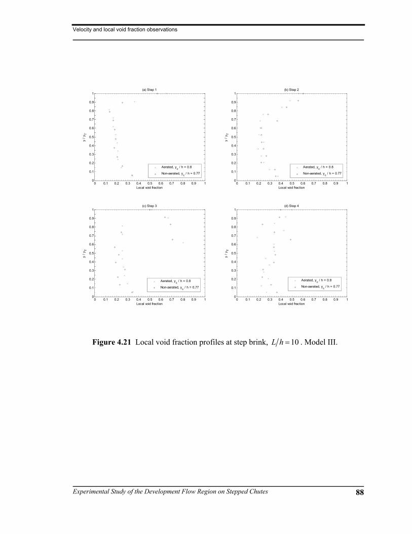
Velocity and local void fraction observations
Experimental Study of the Development Flow Region on Stepped Chutes 88
0 0.1 0.2 0.3 0.4 0.5 0.6 0.7 0.8 0.9 10
0.1
0.2
0.3
0.4
0.5
0.6
0.7
0.8
0.9
1(a) Step 1
y / y
T
Local void fraction
Aerated, yc / h = 0.8
Non-aerated, yc / h = 0.77
0 0.1 0.2 0.3 0.4 0.5 0.6 0.7 0.8 0.9 10
0.1
0.2
0.3
0.4
0.5
0.6
0.7
0.8
0.9
1(b) Step 2
y / y
T
Local void fraction
Aerated, yc / h = 0.8
Non-aerated, yc / h = 0.77
0 0.1 0.2 0.3 0.4 0.5 0.6 0.7 0.8 0.9 10
0.1
0.2
0.3
0.4
0.5
0.6
0.7
0.8
0.9
1(c) Step 3
y / y
T
Local void fraction
Aerated, yc / h = 0.8
Non-aerated, yc / h = 0.77
0 0.1 0.2 0.3 0.4 0.5 0.6 0.7 0.8 0.9 10
0.1
0.2
0.3
0.4
0.5
0.6
0.7
0.8
0.9
1(d) Step 4
y / y
T
Local void fraction
Aerated, yc / h = 0.8
Non-aerated, yc / h = 0.77
Figure 4.21 Local void fraction profiles at step brink, 10L h = . Model III.

Velocity and local void fraction observations
Experimental Study of the Development Flow Region on Stepped Chutes 89
0 0.1 0.2 0.3 0.4 0.5 0.6 0.7 0.8 0.9 10
0.1
0.2
0.3
0.4
0.5
0.6
0.7
0.8
0.9
1(a) Step 1
y / y
T
Local void fraction
Model II, yc / h = 0.78
Model III, yc / h = 0.8
0 0.1 0.2 0.3 0.4 0.5 0.6 0.7 0.8 0.9 10
0.1
0.2
0.3
0.4
0.5
0.6
0.7
0.8
0.9
1(b) Step 2
y / y
T
Local void fraction
Model II, yc / h = 0.78
Model III, yc / h = 0.8
0 0.1 0.2 0.3 0.4 0.5 0.6 0.7 0.8 0.9 10
0.1
0.2
0.3
0.4
0.5
0.6
0.7
0.8
0.9
1(c) Step 3
y / y
T
Local void fraction
Model II, yc / h = 0.78
Model III, yc / h = 0.8
0 0.1 0.2 0.3 0.4 0.5 0.6 0.7 0.8 0.9 1
0
0.1
0.2
0.3
0.4
0.5
0.6
0.7
0.8
0.9
1(d) Step 4
y / y
T
Local void fraction
Model II, yc / h = 0.78
Model III, yc / h = 0.8
Figure 4.22 Comparison of local void fraction profiles with aerated flows
at step brinks. Model II at 5L h = , Model III at 10L h = .

Velocity and local void fraction observations
Experimental Study of the Development Flow Region on Stepped Chutes 90
0 0.1 0.2 0.3 0.4 0.5 0.6 0.7 0.8 0.9 10
0.1
0.2
0.3
0.4
0.5
0.6
0.7
0.8
0.9
1(a) Step 1
y / y
T
Local void fraction
Model II, yc / h = 0.5
Model III, yc / h = 0.49
0 0.1 0.2 0.3 0.4 0.5 0.6 0.7 0.8 0.9 10.1
0.2
0.3
0.4
0.5
0.6
0.7
0.8
0.9
1(b) Step 2
y / y
T
Local void fraction
Model II, yc / h = 0.5
Model III, yc / h = 0.49
0 0.1 0.2 0.3 0.4 0.5 0.6 0.7 0.8 0.9 10
0.1
0.2
0.3
0.4
0.5
0.6
0.7
0.8
0.9
1(c) Step 3
y / y
T
Local void fraction
Model II, yc / h = 0.5
Model III, yc / h = 0.49
0 0.1 0.2 0.3 0.4 0.5 0.6 0.7 0.8 0.9 10
0.1
0.2
0.3
0.4
0.5
0.6
0.7
0.8
0.9
1(d) Step 4
y / y
T
Local void fraction
Model II, yc / h = 0.5
Model III, yc / h = 0.49
Figure 4.23 Comparison of local void fraction profiles with non-aerated
flows at step brinks. Model II at 5L h = , Model III at 10L h = .
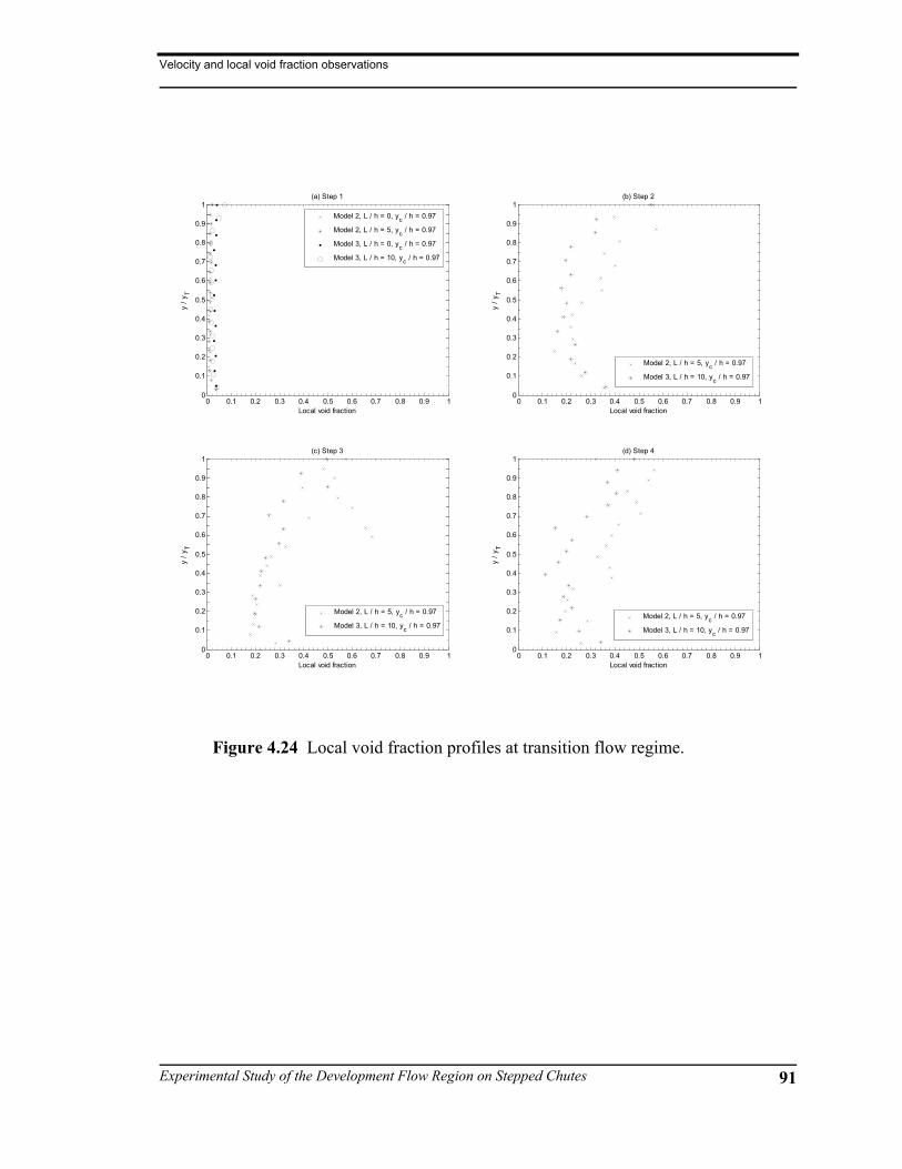
Velocity and local void fraction observations
Experimental Study of the Development Flow Region on Stepped Chutes 91
0 0.1 0.2 0.3 0.4 0.5 0.6 0.7 0.8 0.9 10
0.1
0.2
0.3
0.4
0.5
0.6
0.7
0.8
0.9
1(a) Step 1
Local void fraction
y / y
T
Model 2, L / h = 0, yc / h = 0.97
Model 2, L / h = 5, yc / h = 0.97
Model 3, L / h = 0, yc / h = 0.97
Model 3, L / h = 10, yc / h = 0.97
0 0.1 0.2 0.3 0.4 0.5 0.6 0.7 0.8 0.9 10
0.1
0.2
0.3
0.4
0.5
0.6
0.7
0.8
0.9
1(b) Step 2
Local void fraction
y / y
T
Model 2, L / h = 5, yc / h = 0.97
Model 3, L / h = 10, yc / h = 0.97
0 0.1 0.2 0.3 0.4 0.5 0.6 0.7 0.8 0.9 10
0.1
0.2
0.3
0.4
0.5
0.6
0.7
0.8
0.9
1(c) Step 3
Local void fraction
y / y
T
Model 2, L / h = 5, yc / h = 0.97
Model 3, L / h = 10, yc / h = 0.97
0 0.1 0.2 0.3 0.4 0.5 0.6 0.7 0.8 0.9 10
0.1
0.2
0.3
0.4
0.5
0.6
0.7
0.8
0.9
1(d) Step 4
Local void fraction
y / y
T
Model 2, L / h = 5, yc / h = 0.97
Model 3, L / h = 10, yc / h = 0.97
Figure 4.24 Local void fraction profiles at transition flow regime.

Velocity and local void fraction observations
Experimental Study of the Development Flow Region on Stepped Chutes 92
0 0.1 0.2 0.3 0.4 0.5 0.6 0.7 0.8 0.9 10
0.1
0.2
0.3
0.4
0.5
0.6
0.7
0.8
0.9
1(a) Step 1
Local void fraction
y / y
T
Model 2, L / h = 0, yc / h = 1.6
Model 2, L / h = 5, yc / h = 1.6
Model 3, L / h = 0, yc / h = 1.6
Model 3, L / h = 10, yc / h = 1.6
0 0.1 0.2 0.3 0.4 0.5 0.6 0.7 0.8 0.9 10
0.1
0.2
0.3
0.4
0.5
0.6
0.7
0.8
0.9
1(b) Step 2
Local void fraction
y / y
T
Model 2, L / h = 5, yc / h = 1.6
Model 3, L / h = 10, yc / h = 1.6
0 0.1 0.2 0.3 0.4 0.5 0.6 0.7 0.8 0.9 10
0.1
0.2
0.3
0.4
0.5
0.6
0.7
0.8
0.9
1(c) Step 3
Local void fraction
y / y
T
Model 2, L / h = 5, yc / h = 1.6
Model 3, L / h = 10, yc / h = 1.6
0 0.1 0.2 0.3 0.4 0.5 0.6 0.7 0.8 0.9 10
0.1
0.2
0.3
0.4
0.5
0.6
0.7
0.8
0.9
1(d) Step 4
Local void fraction
y / y
T
Model 2, L / h = 5, yc / h = 1.6
Model 3, L / h = 10, yc / h = 1.6
Figure 4.25 Local void fraction profile at skimming flow regime.

Pressure observations
Experimental Study of the Development Flow Region on Stepped Chutes 93
Chapter 5 Pressure observations
5.1 Introduction
The results of the pressure observation carried out on the three studied models are
presented in this chapter. Initially, observations regarding the filling up process of the
step cavity are presented. Later the measurements and the results on the step tread and on
the step riser are given. Following this, observations and comments regarding the
recirculating pool are presented.
5.2 Step cavity observations
The step cavity corresponds to the area enclosed by the lower nappe of the water
jet and the two faces of a step. Within the step cavity two sections are distinguished: the
recirculating pool and the air pocket. The recirculating pool is formed by the water that
gets diverted towards the step riser when the water jet strikes the step tread. The air
pocket is the volume of air entrapped by the water jet, the recirculating pool and the step;

Pressure observations
Experimental Study of the Development Flow Region on Stepped Chutes 94
this pocket can be aerated or non-aerated depending on whether or not aeration is
provided.
The water level in the recirculating pool increases as the discharge increases and
therefore the air pocket slowly vanishes. The air pocket can also vanish if aeration is not
provided, in this case, the air is entrained into the flow and the water jet deflects towards
the step riser as the air pocket diminishes. Figure 5.1 presents the limit discharge –
expressed as cy h , where the air pocket disappears on the four initial steps of the three
models studied. This figure indicates that at step 1 the condition of the step cavity affects
significantly the values at which the air pocket disappears. In contrast, at steps 2, 3 and 4,
there is no significant difference between the aerated and non-aerated condition for the
chute slopes studied. This is an indication that after the first step, the water nappe is
sufficiently broken to allow air into the cavity.
The value of cy h at which step cavities become filled with water seems to have
a dependency on the chute slope. Figure 5.2 presents such an effect for a constant step
height of 15 cm. In the case of aerated flows (Figure 5.2a), step 1 presents a linear trend,
i.e., as the slope increases so does the value of cy h at which the step becomes full of
water. In contrast, steps 2, 3 and 4 present a concave trend, where the maximum values
of cy h were observed at a chute slope of 5 :1H V ( )11.3θ = ° , i.e., the filling up process
of the step cavity was slower at this slope. Furthermore, the tendency of these steps as
the slope decreases in the rising limb of the curve ( )11.3θ < ° is to converge towards the
value of step 1, which suggests that the step tread would be long enough so there would
be no interference between steps and each step would eventually behave independently.

Pressure observations
Experimental Study of the Development Flow Region on Stepped Chutes 95
In the decreasing limb ( )11.3θ > ° , however, there is no clear tendency and this disparity
is likely to be caused by the deflection of the water jet or perhaps the by the water jet
overshooting the step, although this situation was not observed.
In the case of non-aerated step cavities (Figure 5.2b), the first step became filled
with water at a minimum discharge since the air pocket was depleted by the entrainment
of air into the flow, therefore, this step is not shown in Figure 5.2b. Step 2 on the other
hand, shows a convex tendency with a minimum value of cy h at 5 :1H V , while Steps 3
and 4 a concave trend. Once again, at slopes smaller than 11.3θ = ° the steps tend to
converge whereas at larger slopes the tendency is not clear. Finally, it is worth
mentioning that on the three slopes analyzed in this study the four steps did not become
filled with water at the same value, but rather in a progressive order, which is an
indication that the preceding upstream flow conditions significantly affected the behavior
of each step.
5.3 Pressure observations on step treads
Several pressure measurements were carried out on the initial four steps of each
model. On Model I, seven pressure ports were installed along the each step tread and
measurements were carried out with aeration provided into the step cavity. On Models II
and III, eight ports were installed and measurements were taken for aerated and non-
aerated step cavities. Table 5.1 shows the location iL h of the pressure ports where iL is
the horizontal distance from the step riser.

Pressure observations
Experimental Study of the Development Flow Region on Stepped Chutes 96
Table 5.1 Location of pressure ports on step treads.
Model slope Pressure port location ( )iL h
3.5 :1H V 0.18, 0.35, 0.70, 1.05, 1.40, 2.45, 3.15
5 :1H V 0.25, 0.50, 1.00, 1.50, 2.00, 2.75, 3.75, 4.75
10 :1H V 0.50, 1.00, 1.50, 2.00, 3.00, 4.00, 5.50, 9.50
As mentioned before, pressure measurements along the step tread were carried out
for the conditions of an aerated and non-aerated step cavity. Measurements were taken at
a frequency of 200 Hz during 50 seconds and the data acquisition card was set to a
precision of 4.88± mV. Figures 5.3 to 5.5 show a selection of results for the three
models. Measurements indicated that the condition of the step cavity does not affect
significantly the pressure profile downstream of the jet impact. Upstream of the jet
impact, at the recirculating pool, there was however, a slight variation of the pressure
levels where the non-aerated condition produced slightly larges values. These larger
values are due to the lower pressure conditions which tend to increase the water depths
within the recirculating pool. Similar results were observed on Models II and III.
On the other hand, a comparison between the steps of a given model (Figures 5.6
to 5.8) yielded a diversity of results. In the case of Model I ( )3.5 :1H V the data
indicated that there is no similarity of the pressure profile between the steps of the model,
i.e., each step presented a different pressure profile. Model II ( )5 :1H V showed that at
low and intermediate discharges the pressure profiles on each step were different as well.
However, at large discharges the recorded measurements suggested a similar pressure
Pressure observations
Experimental Study of the Development Flow Region on Stepped Chutes 97
profile at steps 2, 3 and 4 but not at step 1. In the case of Model III ( )10 :1H V , the
measured pressure profiles were similar on all four steps. This might indicate that in the
range of chute slope ( )5.7 11.3θ° ≤ ≤ ° there is a change in the hydraulic behavior of a
stepped spillway, which is reflected by a similar pressure distribution along the step tread.
This effect is initially felt at approximately 11.3θ = ° when large discharges are flowing
but it is completely dominant at a slope ( )θ of about 5.7° .
Finally, a comparison of the results for a given step for each of the different
models is shown in Figures 5.9 to 5.12. On step 1, the three models presented a similar
pressure profile at low flows but this similitude disappeared at intermediate and large
discharges. Conversely, the resemblance on step 2 is stronger at large flows than at low
discharges, which is opposite to the behavior observed for step 1. Steps 3 and 4 however,
presented similar pressure profiles for all three models. Therefore it seems, that there is
no conclusive typical pressure profile between the models, where each model seems to
behave in a characteristic way with some similarities but not sufficient to determine a
unique pressure profile. There is nevertheless, a pattern profile on the step treads, which
moves in the downstream direction on the step tread as the discharge increases. This
pattern of pressure profile initiates with intermediate pressure values at the recirculating
pool, the values then start to increases as iL approaches the point of jet impact, where the
pressure level reaches a maximum. Once iL passes the jet impact point, the pressure
level starts to decrease until a plateau level is reached, which holds until the step brink.
The magnitude of pressure on the plateau is lower than it is in the recirculating pool. The
Pressure observations
Experimental Study of the Development Flow Region on Stepped Chutes 98
location of the jet impact point varies with the step and slope characteristics and it was
observed to be in the range of 1.5 3h≤ ≤ .
5.4 Pressure measurements on step risers
As in the case of the step tread, measurements on the step risers were carried out
with and without aeration in the step cavity. Similarly to the step treads, the sampling
rate on the data acquisition was 200 Hz and it lasted for 50 seconds. Pressure ports were
located at several points along the height of the steps as table 5.2 shows, where *y is the
upward distance from the step tread.
Measurements within a model displayed a similar pressure profile for the aerated
and non-aerated condition (Figures 5.13 to 5.15) and larger pressure were observed at
larger flows. On Model I, the data indicate that the profile was not linear but rather has a
saw shape. This shape is more accentuated with the non-aerated condition, where
slightly smaller pressures were recorded on some of the ports. Similarly to Model I, the
measurements on Model II also defined a saw shape, indistinctively of the condition of
the step cavity. For Model III, the profiles were similar for both aerated and non-aerated
measurements but in contrast to Model I and II, the shape of the profile is more linear
(but not hydrostatic), that is, the saw pattern is substantially less noticeable, with the
exception of step 3. This change in pressure profile reinforces the idea that between
slopes of 5.6° to 11.3° there is a change in the hydraulic behavior of a stepped chute, for
both the aerated and non-aerated condition.

Pressure observations
Experimental Study of the Development Flow Region on Stepped Chutes 99
Table 5.2 Location of pressure ports on the step risers.
Step 1 ( )*y h Step 2 ( )*y h
Model I 0.06, 0.16, 0.32, 0.48, 0.64, 0.80, 0.96 0.06, 0.16, 0.33, 0.49, 0.66, 0.82, 0.94
Model II 0.10, 0.19, 0.30, 0.39, 0.49, 0.59,
0.68, 0.78
0.09, 0.20, 0.30, 0.39, 0.49, 0.59,
0.69, 0.79
Model III 0.10, 0.20, 0.30, 0.39, 0.49, 0.59,
0.69, 0.79
0.11, 0.21, 0.30, 0.40, 0.49, 0.59,
0.69, 0.78
Step 3 ( )*y h Step 4 ( )*y h
Model I 0.06, 0.16, 0.33, 0.49, 0.65, 0.82, 0.95 0.06, 0.16, 0.33, 0.49, 0.66, 0.82, 0.94
Model II 0.10, 0.20, 0.30, 0.40, 0.50, 0.60,
0.70, 0.79
0.10, 0.20, 0.30, 0.40, 0.50, 0.59,
0.69, 0.79
Model III 0.11, 0.21, 0.30, 0.40, 0.50, 0.60,
0.70, 0.80
0.10, 0.20, 0.29, 0.39, 0.48, 0.58,
0.67, 0.77
In spite of the similitude between the aerated and non-aerated condition within a
given model, the pressure profiles on each step are not similar. In Model I for example
(see Figure 5.16), the four steps presented the saw shape but with different magnitudes of
pressure. Furthermore, at intermediate flows, steps 1, 3 and 4 presented a more uniform
shape while step 2 retained the saw form. For the case of larger discharges, steps 1 and 2
again showed the saw shape while steps 3 and 4 a uniform profile.
Model II (Figure 5.17) on the other hand, presented similar saw profiles on the
four steps for all flow conditions. Interestingly, step 1 gave the largest pressure values
while step 4 the smallest; steps 2 and 3 presented intermediate pressure values in a

Pressure observations
Experimental Study of the Development Flow Region on Stepped Chutes 100
descended fashion. Measurements on Model III (Figure 5.18) indicated a more similar
and uniform profile on all steps and flow conditions; nevertheless, there were still some
signs of the saw shape especially on step 3.
Finally, a comparison of the results of a given step (Figure 5.19 to 5.22) shows no
correlation between the observed pressure magnitudes.
The observed saw profile was not expected and it was initially thought to be an
instrumentation or numerical error. Nevertheless, after extensive revisions of the post
processing procedures numerical error was discarded as a source of this observed
pressure variation. Instrumentation error was discarded as the source of the observed
pressure variation by the fact that vertical profiles on the steps were obtained for a variety
of situations as well as the fact that tests on the pressure transducer were carried out
before and after the runs on each step were completed. A more detailed study of the
pressure profile should bring light into the theoretical justification of the observed saw
profile.
5.5 Pools depths observations
Pool depths correspond to the water level on the recirculating pool area which
were measured with respect to the step tread. Figure 5.23 shows the observed pool depth
py for different discharges on the four steps of all three models for the aerated step
cavity condition. This figure assumes that the average water levels on the pool are equal
to the observed pressure levels on ports 1 to 3 on Model I and, ports 1 and 2 on Models II
and III. It would be expected that a correlation should be presented in at least step 1,

Pressure observations
Experimental Study of the Development Flow Region on Stepped Chutes 101
since it is the step that resembles a drop structure. Nevertheless, no such correlation was
distinguished on step 1, or on steps 2, 3 or 4.
When the air pocket was presented it was also observed that the recirculating pool
became shallower and elongated in downstream direction; a fact that was more evident at
the smallest slope tested but it was also noticeable at 11.3θ = ° . The water level on the
pool fluctuated intensively, which might have had an influence on the observed saw
shape of the riser pressure profile. These fluctuations were more intensive at the steeper
slope and it was also observed that on average, the water level was slightly inclined
towards the point of jet impact, i.e., larger water depths on the riser zone and lower
depths close to the jet impact.
Finally, when the step cavity became full of water two symmetric spiral vortices
were observed in the vicinity of the step riser, these vortices had a flow direction towards
the sides of the models in the area closest to the riser and in the ascending flow direction.

Pressure observations
Experimental Study of the Development Flow Region on Stepped Chutes 102
0 1 2 3 4 50
0.2
0.4
0.6
0.8
1
1.2
1.4
1.6
1.8
Step
y c / h
a) Model I, 3.5H:1V
Run A8Run A7NA-TRATRA-SK
0 1 2 3 4 50
0.2
0.4
0.6
0.8
1
1.2
1.4
1.6
1.8
Step
y c / h
b) Model II, 5H:1V
Run B15-B18Run B1NA-TRATRA-SK
0 1 2 3 4 50
0.2
0.4
0.6
0.8
1
1.2
1.4
1.6
1.8
Step
y c / h
c) Model III, 10H:1V
Run C19Run C1NA-TRATRA-SK
Figure 5.1 Observed points where the air pocket vanishes.
Aerated condition: runs A8, B15-B18 and C1. Non-
aerated condition: runs A7, B1 and C1.

Pressure observations
Experimental Study of the Development Flow Region on Stepped Chutes 103
4 6 8 10 12 14 16 180.6
0.8
1
1.2
1.4
1.6
1.8
2
Chute slope (degrees)
y c / h
a) Aerated flows
Step 1Step 2Step 3Step 4NA-TRATRA-SK
4 6 8 10 12 14 16 180.6
0.8
1
1.2
1.4
1.6
1.8
2
Chute slope (degrees)
y c / h
b) Non-aerated flows
Step 2Step 3Step 4NA-TRATRA-SK
Figure 5.2 Slope effect on the presence of the air pocket.
Constant step height of 15 cm.
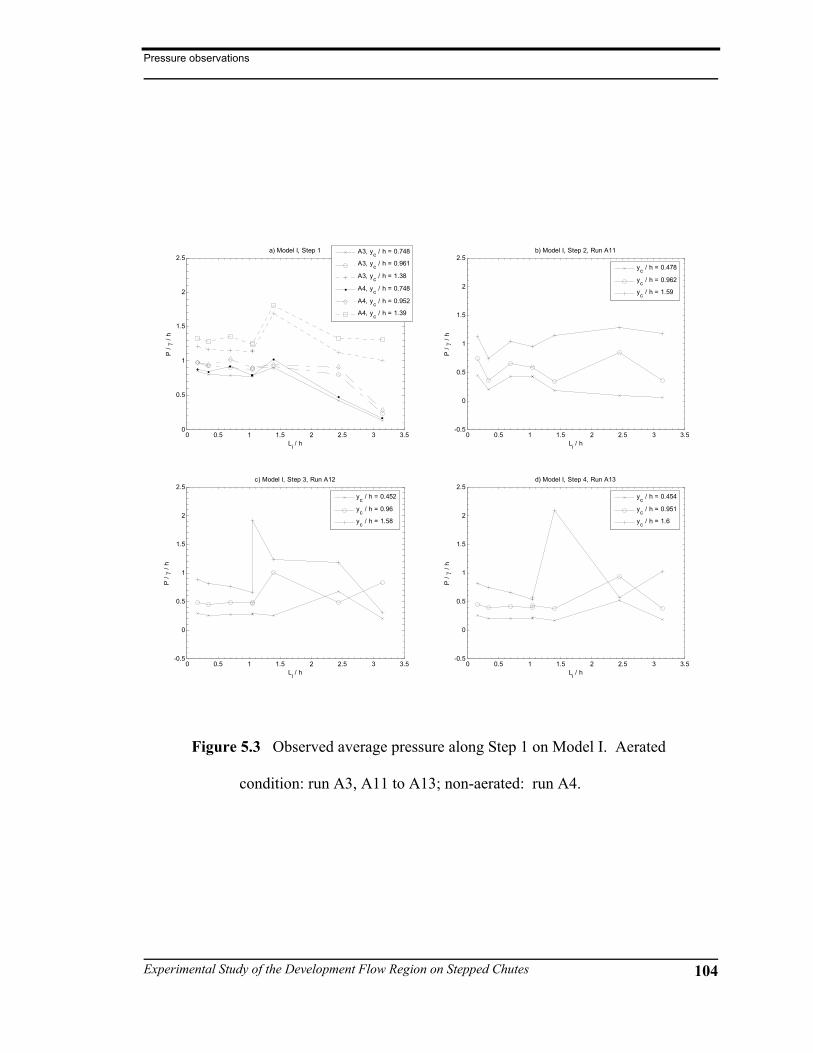
Pressure observations
Experimental Study of the Development Flow Region on Stepped Chutes 104
0 0.5 1 1.5 2 2.5 3 3.50
0.5
1
1.5
2
2.5
Li / h
P / γ
/ h
a) Model I, Step 1 A3, yc / h = 0.748
A3, yc / h = 0.961
A3, yc / h = 1.38
A4, yc / h = 0.748
A4, yc / h = 0.952
A4, yc / h = 1.39
0 0.5 1 1.5 2 2.5 3 3.5-0.5
0
0.5
1
1.5
2
2.5
Li / hP
/ γ
/ h
b) Model I, Step 2, Run A11
yc / h = 0.478
yc / h = 0.962
yc / h = 1.59
0 0.5 1 1.5 2 2.5 3 3.5-0.5
0
0.5
1
1.5
2
2.5
Li / h
P / γ
/ h
c) Model I, Step 3, Run A12
yc / h = 0.452
yc / h = 0.96
yc / h = 1.58
0 0.5 1 1.5 2 2.5 3 3.5-0.5
0
0.5
1
1.5
2
2.5
Li / h
P / γ
/ h
d) Model I, Step 4, Run A13
yc / h = 0.454
yc / h = 0.951
yc / h = 1.6
Figure 5.3 Observed average pressure along Step 1 on Model I. Aerated
condition: run A3, A11 to A13; non-aerated: run A4.

Pressure observations
Experimental Study of the Development Flow Region on Stepped Chutes 105
0 0.5 1 1.5 2 2.5 3 3.5 4 4.5 5-0.5
0
0.5
1
1.5
2
2.5
Li / h
P / γ
/ h
a) Model II, Step 1 B11, yc / h = 0.489
B11, yc / h = 0.863
B11, yc / h = 1.64
B10, yc / h = 0.515
B10, yc / h = 0.908
B10, yc / h = 1.64
0 0.5 1 1.5 2 2.5 3 3.5 4 4.5 5-0.5
0
0.5
1
1.5
2
2.5
Li / h
P / γ
/ h
b) Model II, Step 2B12, yc / h = 0.499
B12, yc / h = 0.871
B12, yc / h = 1.64
B9, yc / h = 0.508
B9, yc / h = 0.905
B9, yc / h = 1.63
0 0.5 1 1.5 2 2.5 3 3.5 4 4.5 5-0.5
0
0.5
1
1.5
2
2.5
Li / h
P / γ
/ h
c) Model II, Step 3B13, yc / h = 0.501
B13, yc / h = 0.877
B13, yc / h = 1.65
B8, yc / h = 0.507
B8, yc / h = 0.905
B8, yc / h = 1.65
0 0.5 1 1.5 2 2.5 3 3.5 4 4.5 5-0.5
0
0.5
1
1.5
2
2.5
Li / h
P / γ
/ hd) Model II, Step 4
B14, yc / h = 0.501
B14, yc / h = 0.876
B14, yc / h = 1.63
B7, yc / h = 0.506
B7, yc / h = 0.913
B7, yc / h = 1.62
Figure 5.4 Measured average pressure on step treads on Model II.
Aerated condition: run B11 to B14; non-aerated condition: runs
B7 to B10.

Pressure observations
Experimental Study of the Development Flow Region on Stepped Chutes 106
0 1 2 3 4 5 6 7 8 9 10-0.5
0
0.5
1
1.5
2
2.5
Li / h
P / γ
/ h
a) Model III, Step 1
C11, yc / h = 0.512
C11, yc / h = 0.984
C11, yc / h = 1.65
C7, yc / h = 0.514
C7, yc / h = 0.979
C7, yc / h = 1.65
0 1 2 3 4 5 6 7 8 9 10-0.5
0
0.5
1
1.5
2
2.5
Li / hP
/ γ
/ h
b) Model III, Step 2
C12, yc / h = 0.488
C12, yc / h = 0.943
C12, yc / h = 1.61
C8, yc / h = 0.492
C8, yc / h = 0.956
C8, yc / h = 1.6
0 1 2 3 4 5 6 7 8 9 10-0.5
0
0.5
1
1.5
2
2.5
Li / h
P / γ
/ h
c) Model III, Step 3
C13, yc / h = 0.638
C13, yc / h = 0.892
C13, yc / h = 1.66
C9, yc / h = 0.653
C9, yc / h = 0.902
C9, yc / h = 1.65
0 1 2 3 4 5 6 7 8 9 10-0.5
0
0.5
1
1.5
2
2.5
Li / h
P / γ
/ h
d) Model III, Step 4
C14, yc / h = 0.473
C14, yc / h = 1.02
C14, yc / h = 1.58
C10, yc / h = 0.477
C10, yc / h = 1.02
C10, yc / h = 1.58
Figure 5.5 Measured average pressure on step treads on Model III.
Aerated condition: run C11 to C14; non-aerated condition: runs
C7 to C10.

Pressure observations
Experimental Study of the Development Flow Region on Stepped Chutes 107
0 0.5 1 1.5 2 2.5 3 3.5-0.5
0
0.5
1
1.5
2
2.5
Li / hP
/ γ
/ h
a) Nappe flow regime
Step 1, A3, yc / h = 0.447
Step 2, A11, yc / h = 0.478
Step 3, A12, yc / h = 0.452
Step 4, A13, yc / h = 0.454
0 0.5 1 1.5 2 2.5 3 3.5-0.5
0
0.5
1
1.5
2
2.5
Li / h
P / γ
/ h
b) Transition flow regime
Step 1, A3, yc / h = 0.961
Step 2, A11, yc / h = 0.962
Step 3, A12, yc / h = 0.96
Step 4, A13, yc / h = 0.951
0 0.5 1 1.5 2 2.5 3 3.5-0.5
0
0.5
1
1.5
2
2.5
Li / h
P / γ
/ h
c) Skimming flow regime
Step 1, A3, yc / h = 1.57
Step 2, A11, yc / h = 1.59
Step 3, A12, yc / h = 1.58
Step 4, A13, yc / h = 1.6
Figure 5.6 Recorded pressure on the treads of Model I,
aerated flow condition.

Pressure observations
Experimental Study of the Development Flow Region on Stepped Chutes 108
0 0.5 1 1.5 2 2.5 3 3.5 4 4.5 5-0.5
0
0.5
1
1.5
2
2.5
Li / h
P / γ
/ h
a) Nappe flow regime
Step 1, B11, yc / h = 0.489
Step 2, B12, yc / h = 0.499
Step 3, B13, yc / h = 0.501
Step 4, B14, yc / h = 0.501
0 0.5 1 1.5 2 2.5 3 3.5 4 4.5 5-0.5
0
0.5
1
1.5
2
2.5
Li / h
P / γ
/ h
d) Nappe flow regime
Step 1, B10, yc / h = 0.515
Step 2, B9, yc / h = 0.508
Step 3, B8, yc / h = 0.507
Step 4, B7, yc / h = 0.506
0 0.5 1 1.5 2 2.5 3 3.5 4 4.5 5-0.5
0
0.5
1
1.5
2
2.5
Li / h
P / γ
/ h
b) Transition flow regime
Step 1, B11, yc / h = 0.957
Step 2, B12, yc / h = 0.963
Step 3, B13, yc / h = 0.976
Step 4, B14, yc / h = 0.969
0 0.5 1 1.5 2 2.5 3 3.5 4 4.5 5-0.5
0
0.5
1
1.5
2
2.5
Li / h
P / γ
/ h
e) Transition flow regime
Step 1, B10, yc / h = 1.01
Step 2, B9, yc / h = 0.99
Step 3, B8, yc / h = 1.01
Step 4, B7, yc / h = 1.01
0 0.5 1 1.5 2 2.5 3 3.5 4 4.5 5-0.5
0
0.5
1
1.5
2
2.5
Li / h
P / γ
/ h
c) Skimming flow regime
Step 1, B11, yc / h = 1.64
Step 2, B12, yc / h = 1.64
Step 3, B13, yc / h = 1.65
Step 4, B14, yc / h = 1.63
0 0.5 1 1.5 2 2.5 3 3.5 4 4.5 5-0.5
0
0.5
1
1.5
2
2.5
Li / h
P / γ
/ h
f) Skimming flow regime
Step 1, B10, yc / h = 1.64
Step 2, B9, yc / h = 1.63
Step 3, B8, yc / h = 1.65
Step 4, B7, yc / h = 1.62
Figure 5.7 Average pressure on the treads of Model II. Aerated cavity:
figures a to c; Non-aerated cavities: figures d to f.

Pressure observations
Experimental Study of the Development Flow Region on Stepped Chutes 109
0 1 2 3 4 5 6 7 8 9 10-0.5
0
0.5
1
1.5
2
2.5
Li / h
P / γ
/ h
a) Nappe flow regime
Step 1, C11, yc / h = 0.512
Step 2, C12, yc / h = 0.488
Step 3, C13, yc / h = 0.501
Step 4, C14, yc / h = 0.473
0 1 2 3 4 5 6 7 8 9 10-0.5
0
0.5
1
1.5
2
2.5
Li / h
P / γ
/ h
d) Nappe flow regime
Step 1, C7, yc / h = 0.514
Step 2, C8, yc / h = 0.492
Step 3, C9, yc / h = 0.521
Step 4, C10, yc / h = 0.477
0 1 2 3 4 5 6 7 8 9 10-0.5
0
0.5
1
1.5
2
2.5
Li / h
P / γ
/ h
b) Transition flow regime
Step 1, C11, yc / h = 0.984
Step 2, C12, yc / h = 0.943
Step 3, C13, yc / h = 0.986
Step 4, C14, yc / h = 0.93
0 1 2 3 4 5 6 7 8 9 10-0.5
0
0.5
1
1.5
2
2.5
Li / h
P / γ
/ h
e) Transition flow regime
Step 1, C7, yc / h = 0.979
Step 2, C8, yc / h = 0.956
Step 3, C9, yc / h = 1
Step 4, C10, yc / h = 0.965
0 1 2 3 4 5 6 7 8 9 10-0.5
0
0.5
1
1.5
2
2.5
Li / h
P / γ
/ h
c) Skimming flow regime
Step 1, C11, yc / h = 1.65
Step 2, C12, yc / h = 1.61
Step 3, C13, yc / h = 1.66
Step 4, C14, yc / h = 1.58
0 1 2 3 4 5 6 7 8 9 10-0.5
0
0.5
1
1.5
2
2.5
Li / h
P / γ
/ h
f) Skimming flow regime
Step 1, C7, yc / h = 1.65
Step 2, C8, yc / h = 1.6
Step 3, C9, yc / h = 1.65
Step 4, C10, yc / h = 1.58
Figure 5.8 Average pressure on the treads of Model III. Aerated cavity:
figures a to c; Non-aerated cavities: figures d to f.

Pressure observations
Experimental Study of the Development Flow Region on Stepped Chutes 110
0 1 2 3 4 5 6 7 8 9 10-0.5
0
0.5
1
1.5
2
2.5
Li / h
P / γ
/ h
a) Step 1, nappe flow regime, aerated
Model I, A3, yc / h = 0.648
Model II, B11, yc / h = 0.623
Model III, C11, yc / h = 0.647
0 1 2 3 4 5 6 7 8 9 10-0.5
0
0.5
1
1.5
2
2.5
Li / h
P / γ
/ h
d) Step 1, nappe flow regime, non-aerated
Model I, A4, yc / h = 0.453
Model II, B10, yc / h = 0.515
Model III, C7, yc / h = 0.514
0 1 2 3 4 5 6 7 8 9 10-0.5
0
0.5
1
1.5
2
2.5
Li / h
P / γ
/ h
b) Step 1, transition flow regime, aerated
Model I, A3, yc / h = 0.961
Model II, B11, yc / h = 0.957
Model III, C11, yc / h = 0.984
0 1 2 3 4 5 6 7 8 9 10-0.5
0
0.5
1
1.5
2
2.5
Li / h
P / γ
/ h
e) Step 1, transition flow regime, non-aerated
Model I, A4, yc / h = 0.844
Model II, B10, yc / h = 0.908
Model III, C7, yc / h = 0.895
0 1 2 3 4 5 6 7 8 9 10-0.5
0
0.5
1
1.5
2
2.5
Li / h
P / γ
/ h
c) Step 1, skimmming flow regime, aerated
Model I, A3, yc / h = 1.57
Model II, B11, yc / h = 1.64
Model III, C11, yc / h = 1.65
0 1 2 3 4 5 6 7 8 9 10-0.5
0
0.5
1
1.5
2
2.5
Li / h
P / γ
/ h
f) Step 1, skimmming flow regime, non-aerated
Model I, A4, yc / h = 1.55
Model II, B10, yc / h = 1.64
Model III, C7, yc / h = 1.65
Figure 5.9 Average pressure on the tread of step 1.

Pressure observations
Experimental Study of the Development Flow Region on Stepped Chutes 111
0 1 2 3 4 5 6 7 8 9 10-0.5
0
0.5
1
1.5
2
2.5
Li / h
P / γ
/ h
a) Step 2, nappe flow regime, aerated
Model I, A11, yc / h = 0.478
Model II, B12, yc / h = 0.499
Model III, C12, yc / h = 0.488
0 1 2 3 4 5 6 7 8 9 10-0.5
0
0.5
1
1.5
2
2.5
Li / h
P / γ
/ h
d) Step 2, nappe flow regime, non-aerated
Model II, B9, yc / h = 0.508
Model III, C8, yc / h = 0.492
0 1 2 3 4 5 6 7 8 9 10-0.5
0
0.5
1
1.5
2
2.5
Li / h
P / γ
/ h
b) Step 2, transition flow regime, aerated
Model I, A11, yc / h = 0.962
Model II, B12, yc / h = 0.963
Model III, C12, yc / h = 0.943
0 1 2 3 4 5 6 7 8 9 10-0.5
0
0.5
1
1.5
2
2.5
Li / h
P / γ
/ h
e) Step 2, transition flow regime, non-aerated
Model II, B9, yc / h = 0.99
Model III, C8, yc / h = 0.956
0 1 2 3 4 5 6 7 8 9 10-0.5
0
0.5
1
1.5
2
2.5
Li / h
P / γ
/ h
c) Step 2, skimmming flow regime, aerated
Model I, A11, yc / h = 1.59
Model II, B12, yc / h = 1.64
Model III, C12, yc / h = 1.61
0 1 2 3 4 5 6 7 8 9 10-0.5
0
0.5
1
1.5
2
2.5
Li / h
P / γ
/ h
f) Step 2, skimmming flow regime, non-aerated
Model II, B9, yc / h = 1.63
Model III, C8, yc / h = 1.6
Figure 5.10 Average pressure on the tread of step 2.

Pressure observations
Experimental Study of the Development Flow Region on Stepped Chutes 112
0 1 2 3 4 5 6 7 8 9 10-0.5
0
0.5
1
1.5
2
2.5
Li / h
P / γ
/ h
a) Step 3, nappe flow regime, aerated
Model I, A12, yc / h = 0.616
Model II, B13, yc / h = 0.629
Model III, C13, yc / h = 0.638
0 1 2 3 4 5 6 7 8 9 10-0.5
0
0.5
1
1.5
2
2.5
Li / h
P / γ
/ h
d) Step 3, nappe flow regime, non-aerated
Model II, B8, yc / h = 0.659
Model III, C9, yc / h = 0.653
0 1 2 3 4 5 6 7 8 9 10-0.5
0
0.5
1
1.5
2
2.5
Li / h
P / γ
/ h
b) Step 3, transition flow regime, aerated
Model I, A12, yc / h = 0.96
Model II, B13, yc / h = 0.976
Model III, C13, yc / h = 0.986
0 1 2 3 4 5 6 7 8 9 10-0.5
0
0.5
1
1.5
2
2.5
Li / h
P / γ
/ h
e) Step 3, transition flow regime, non-aerated
Model II, B8, yc / h = 1.01
Model III, C9, yc / h = 1
0 1 2 3 4 5 6 7 8 9 10-0.5
0
0.5
1
1.5
2
2.5
Li / h
P / γ
/ h
c) Step 3, skimmming flow regime, aerated
Model I, A12, yc / h = 1.58
Model II, B13, yc / h = 1.65
Model III, C13, yc / h = 1.66
0 1 2 3 4 5 6 7 8 9 10-0.5
0
0.5
1
1.5
2
2.5
Li / h
P / γ
/ h
f) Step 3, skimmming flow regime, non-aerated
Model II, B8, yc / h = 1.65
Model III, C9, yc / h = 1.65
Figure 5.11 Average pressure on the tread of step 3.

Pressure observations
Experimental Study of the Development Flow Region on Stepped Chutes 113
0 1 2 3 4 5 6 7 8 9 10-0.5
0
0.5
1
1.5
2
2.5
Li / h
P / γ
/ h
a) Step 4, nappe flow regime, aerated
Model I, A13, yc / h = 0.604
Model II, B14, yc / h = 0.633
Model III, C14, yc / h = 0.606
0 1 2 3 4 5 6 7 8 9 10-0.5
0
0.5
1
1.5
2
2.5
Li / h
P / γ
/ h
d) Step 4, nappe flow regime, non-aerated
Model II, B7, yc / h = 0.644
Model III, C10, yc / h = 0.623
0 1 2 3 4 5 6 7 8 9 10-0.5
0
0.5
1
1.5
2
2.5
Li / h
P / γ
/ h
b) Step 4, transition flow regime, aerated
Model I, A13, yc / h = 0.951
Model II, B14, yc / h = 0.969
Model III, C14, yc / h = 0.93
0 1 2 3 4 5 6 7 8 9 10-0.5
0
0.5
1
1.5
2
2.5
Li / h
P / γ
/ h
e) Step 4, transition flow regime, non-aerated
Model II, B7, yc / h = 1.01
Model III, C10, yc / h = 0.965
0 1 2 3 4 5 6 7 8 9 10-0.5
0
0.5
1
1.5
2
2.5
Li / h
P / γ
/ h
c) Step 4, skimmming flow regime, aerated
Model I, A13, yc / h = 1.6
Model II, B14, yc / h = 1.63
Model III, C14, yc / h = 1.58
0 1 2 3 4 5 6 7 8 9 10-0.5
0
0.5
1
1.5
2
2.5
Li / h
P / γ
/ h
f) Step 4, skimmming flow regime, non-aerated
Model II, B7, yc / h = 1.62
Model III, C10, yc / h = 1.58
Figure 5.12 Average pressure on the tread of step 4.

Pressure observations
Experimental Study of the Development Flow Region on Stepped Chutes 114
-1 -0.5 0 0.5 1 1.50
0.1
0.2
0.3
0.4
0.5
0.6
0.7
0.8
0.9
1
P / γ / h
y* /
h
a) Model I, Step 1
A1, yc / h = 0.451
A1, yc / h = 0.938
A1, yc / h = 1.55
A2, yc / h = 0.448
A2, yc / h = 0.952
A2, yc / h = 1.54
Figure 5.13 Average pressures on the riser of step 1,
Model I. Aerated step cavity: run A1; non aerated
step cavity: run A2.

Pressure observations
Experimental Study of the Development Flow Region on Stepped Chutes 115
-1 -0.5 0 0.5 1 1.50
0.1
0.2
0.3
0.4
0.5
0.6
0.7
0.8
0.9
1
P / γ / h
y* /
ha) Model II, Step 1
B15, yc / h = 0.51
B15, yc / h = 1.06
B15, yc / h = 1.64
B3, yc / h = 0.507
B3, yc / h = 1.06
B3, yc / h = 1.63
-1 -0.5 0 0.5 1 1.50
0.1
0.2
0.3
0.4
0.5
0.6
0.7
0.8
0.9
1
P / γ / h
y* /
h
b) Model II, Step 2
B16, yc / h = 0.513
B16, yc / h = 1
B16, yc / h = 1.63
B4, yc / h = 0.504
B4, yc / h = 0.995
B4, yc / h = 1.63
-1 -0.5 0 0.5 1 1.50
0.1
0.2
0.3
0.4
0.5
0.6
0.7
0.8
0.9
1
P / γ / h
y* /
h
c) Model II, Step 3
B17, yc / h = 0.51
B17, yc / h = 0.965
B17, yc / h = 1.65
B5, yc / h = 0.514
B5, yc / h = 1
B5, yc / h = 1.64
-1 -0.5 0 0.5 1 1.50
0.1
0.2
0.3
0.4
0.5
0.6
0.7
0.8
0.9
1
P / γ / h
y* /
hd) Model II, Step 4
B18, yc / h = 0.492
B18, yc / h = 0.945
B18 yc / h = 1.43
B6, yc / h = 0.512
B6, yc / h = 0.99
B6, yc / h = 1.43
Figure 5.14 Average pressures on risers of Model II. Aerated step cavity:
runs B15-B18; non aerated step cavity: runs B3-B6.

Pressure observations
Experimental Study of the Development Flow Region on Stepped Chutes 116
-1 -0.5 0 0.5 1 1.50
0.1
0.2
0.3
0.4
0.5
0.6
0.7
0.8
0.9
1
P / γ / h
y* /
h
a) Model III, Step 1
C15, yc / h = 0.493
C15, yc / h = 0.976
C15, yc / h = 1.65
C3, yc / h = 0.509
C3, yc / h = 0.98
C3, yc / h = 1.65
-1 -0.5 0 0.5 1 1.50
0.1
0.2
0.3
0.4
0.5
0.6
0.7
0.8
0.9
1
P / γ / h
y* /
h
b) Model III, Step 2
C16, yc / h = 0.496
C16, yc / h = 0.95
C16, yc / h = 1.6
C4, yc / h = 0.498
C4, yc / h = 0.943
C4, yc / h = 1.41
-1 -0.5 0 0.5 1 1.50
0.1
0.2
0.3
0.4
0.5
0.6
0.7
0.8
0.9
1
P / γ / h
y* /
h
c) Model III, Step 3
C17, yc / h = 0.51
C17, yc / h = 0.888
C17, yc / h = 1.66
C5, yc / h = 0.517
C5, yc / h = 0.889
C5, yc / h = 1.65
-1 -0.5 0 0.5 1 1.50
0.1
0.2
0.3
0.4
0.5
0.6
0.7
0.8
0.9
1
P / γ / h
y* /
h
d) Model III, Step 4
C18, yc / h = 0.618
C18, yc / h = 0.937
C18, yc / h = 1.58
C6, yc / h = 0.61
C6, yc / h = 0.924
C6, yc / h = 1.58
Figure 5.15 Average pressures on risers of Model III. Aerated step
cavity: runs C15-C18; non aerated step cavity: runs C3-C6.

Pressure observations
Experimental Study of the Development Flow Region on Stepped Chutes 117
-1 -0.5 0 0.5 1 1.50
0.1
0.2
0.3
0.4
0.5
0.6
0.7
0.8
0.9
1
P / γ / h
y* /
h
a) Nappe flow regime
Step 1, A1, yc / h = 0.451
Step 2, A11, yc / h = 0.478
Step 3, A12, yc / h = 0.452
Step 4, A13, yc / h = 0.454
-1 -0.5 0 0.5 1 1.50
0.1
0.2
0.3
0.4
0.5
0.6
0.7
0.8
0.9
1
P / γ / h
y* /
h
b) Transition flow regime
Step 1, A1, yc / h = 0.938
Step 2, A11, yc / h = 0.962
Step 3, A12, yc / h = 0.96
Step 4, A13, yc / h = 0.951
-1 -0.5 0 0.5 1 1.50
0.1
0.2
0.3
0.4
0.5
0.6
0.7
0.8
0.9
1
P / γ / h
y* /
h
c) Skimming flow regime
Step 1, A1, yc / h = 1.55
Step 2, A11, yc / h = 1.59
Step 3, A12, yc / h = 1.58
Step 4, A13, yc / h = 1.6
Figure 5.16 Average pressure on the risers of Model I.
Condition of the step cavity: aerated.

Pressure observations
Experimental Study of the Development Flow Region on Stepped Chutes 118
-1 -0.5 0 0.5 1 1.50
0.1
0.2
0.3
0.4
0.5
0.6
0.7
0.8
0.9
1
P / γ / h
y* /
h
a) Nappe flow regime
Step 1, B15, yc / h = 0.51
Step 2, B16, yc / h = 0.513
Step 3, B17, yc / h = 0.51
Step 4, B18, yc / h = 0.492
-1 -0.5 0 0.5 1 1.50
0.1
0.2
0.3
0.4
0.5
0.6
0.7
0.8
0.9
1
P / γ / h
y* /
h
d) Nappe flow regime
Step 1, B3, yc / h = 0.507
Step 2, B4, yc / h = 0.504
Step 3, B5, yc / h = 0.514
Step 4, B6, yc / h = 0.512
-1 -0.5 0 0.5 1 1.50
0.1
0.2
0.3
0.4
0.5
0.6
0.7
0.8
0.9
1
P / γ / h
y* /
h
b) Transition flow regime
Step 1, B15, yc / h = 0.968
Step 2, B16, yc / h = 1
Step 3, B17, yc / h = 0.965
Step 4, B18, yc / h = 0.945
-1 -0.5 0 0.5 1 1.50
0.1
0.2
0.3
0.4
0.5
0.6
0.7
0.8
0.9
1
P / γ / h
y* /
h
e) Transition flow regime
Step 1, B3, yc / h = 0.997
Step 2, B4, yc / h = 0.995
Step 3, B5, yc / h = 1
Step 4, B6, yc / h = 0.99
-1 -0.5 0 0.5 1 1.50
0.1
0.2
0.3
0.4
0.5
0.6
0.7
0.8
0.9
1
P / γ / h
y* /
h
c) Skimming flow regime
Step 1, B15, yc / h = 1.64
Step 2, B16, yc / h = 1.63
Step 3, B17, yc / h = 1.65
Step 4, B18, yc / h = 1.62
-1 -0.5 0 0.5 1 1.50
0.1
0.2
0.3
0.4
0.5
0.6
0.7
0.8
0.9
1
P / γ / h
y* /
h
f) Skimming flow regime
Step 1, B3, yc / h = 1.63
Step 2, B4, yc / h = 1.63
Step 3, B5, yc / h = 1.64
Step 4, B6, yc / h = 1.6
Figure 5.17 Average pressure on the risers of Model II. Aerated step
cavity: figures a to c; non-aerated step cavity: figures d to f.

Pressure observations
Experimental Study of the Development Flow Region on Stepped Chutes 119
-1 -0.5 0 0.5 1 1.50
0.1
0.2
0.3
0.4
0.5
0.6
0.7
0.8
0.9
1
P / γ / h
y* /
h
a) Nappe flow regime
Step 1, C15, yc / h = 0.493
Step 2, C16, yc / h = 0.496
Step 3, C17, yc / h = 0.51
Step 4, C18, yc / h = 0.489
-1 -0.5 0 0.5 1 1.50
0.1
0.2
0.3
0.4
0.5
0.6
0.7
0.8
0.9
1
P / γ / h
y* /
h
d) Nappe flow regime
Step 1, C3, yc / h = 0.509
Step 2, C4, yc / h = 0.498
Step 3, C5, yc / h = 0.517
Step 4, C6, yc / h = 0.475
-1 -0.5 0 0.5 1 1.50
0.1
0.2
0.3
0.4
0.5
0.6
0.7
0.8
0.9
1
P / γ / h
y* /
h
b) Transition flow regime
Step 1, C15, yc / h = 0.976
Step 2, C16, yc / h = 0.95
Step 3, C17, yc / h = 0.978
Step 4, C18, yc / h = 0.937
-1 -0.5 0 0.5 1 1.50
0.1
0.2
0.3
0.4
0.5
0.6
0.7
0.8
0.9
1
P / γ / h
y* /
h
e) Transition flow regime
Step 1, C3, yc / h = 0.98
Step 2, C4, yc / h = 0.943
Step 3, C5, yc / h = 0.989
Step 4, C6, yc / h = 0.924
-1 -0.5 0 0.5 1 1.50
0.1
0.2
0.3
0.4
0.5
0.6
0.7
0.8
0.9
1
P / γ / h
y* /
h
c) Skimming flow regime
Step 1, C15, yc / h = 1.65
Step 2, C16, yc / h = 1.6
Step 3, C17, yc / h = 1.66
Step 4, C18, yc / h = 1.58
-1 -0.5 0 0.5 1 1.50
0.1
0.2
0.3
0.4
0.5
0.6
0.7
0.8
0.9
1
P / γ / h
y* /
h
f) Skimming flow regime
Step 1, C3, yc / h = 1.65
Step 2, C4, yc / h = 1.6
Step 3, C5, yc / h = 1.65
Step 4, C6, yc / h = 1.58
Figure 5.18 Average pressure on the risers of Model III. Aerated step
cavity: figures a to c; non-aerated step cavity: figures d to f.

Pressure observations
Experimental Study of the Development Flow Region on Stepped Chutes 120
-1 -0.5 0 0.5 1 1.50
0.1
0.2
0.3
0.4
0.5
0.6
0.7
0.8
0.9
1
P / γ / h
y* /
ha) Step 1, Nappe flow regime, aerated
Model I, A1, yc / h = 0.451
Model II, B15, yc / h = 0.51
Model III, C15, yc / h = 0.493
-1 -0.5 0 0.5 1 1.50
0.1
0.2
0.3
0.4
0.5
0.6
0.7
0.8
0.9
1
P / γ / h
y* /
h
d) Step 1, Nappe flow regime, non-aerated
Model I, A2, yc / h = 0.448
Model II, B3, yc / h = 0.507
Model III, C3, yc / h = 0.509
-1 -0.5 0 0.5 1 1.50
0.1
0.2
0.3
0.4
0.5
0.6
0.7
0.8
0.9
1
P / γ / h
y* /
h
b) Step 1, Transition flow regime, aerated
Model I, A1, yc / h = 0.938
Model II, B15, yc / h = 0.968
Model III, C15, yc / h = 0.976
-1 -0.5 0 0.5 1 1.50
0.1
0.2
0.3
0.4
0.5
0.6
0.7
0.8
0.9
1
P / γ / h
y* /
h
e) Step 1, Transition flow regime, non-aerated
Model I, A2, yc / h = 0.952
Model II, B3, yc / h = 0.997
Model III, C3, yc / h = 0.98
-1 -0.5 0 0.5 1 1.50
0.1
0.2
0.3
0.4
0.5
0.6
0.7
0.8
0.9
1
P / γ / h
y* /
h
c) Step 1, Skimming flow regime, aerated
Model I, A1, yc / h = 1.55
Model II, B15, yc / h = 1.64
Model III, C15, yc / h = 1.65
-1 -0.5 0 0.5 1 1.50
0.1
0.2
0.3
0.4
0.5
0.6
0.7
0.8
0.9
1
P / γ / h
y* /
h
f) Step 1, Skimming flow regime, non-aerated
Model I, A2, yc / h = 1.54
Model II, B3, yc / h = 1.63
Model III, C3, yc / h = 1.65
Figure 5.19 Average pressure on the riser of step 1.

Pressure observations
Experimental Study of the Development Flow Region on Stepped Chutes 121
-1 -0.5 0 0.5 1 1.50
0.1
0.2
0.3
0.4
0.5
0.6
0.7
0.8
0.9
1
P / γ / h
y* /
h
a) Step 2, Nappe flow regime, aerated
Model I, A11, yc / h = 0.636
Model II, B16, yc / h = 0.657
Model III, C16, yc / h = 0.626
-1 -0.5 0 0.5 1 1.50
0.1
0.2
0.3
0.4
0.5
0.6
0.7
0.8
0.9
1
P / γ / h
y* /
h
d) Step 2, Nappe flow regime, non-aerated
Model II, B4, yc / h = 0.504
Model III, C4, yc / h = 0.498
-1 -0.5 0 0.5 1 1.50
0.1
0.2
0.3
0.4
0.5
0.6
0.7
0.8
0.9
1
P / γ / h
y* /
h
b) Step 2, Transition flow regime, aerated
Model I, A11, yc / h = 0.962
Model II, B16, yc / h = 1
Model III, C16, yc / h = 0.95
-1 -0.5 0 0.5 1 1.50
0.1
0.2
0.3
0.4
0.5
0.6
0.7
0.8
0.9
1
P / γ / h
y* /
h
e) Step 2, Transition flow regime, non-aerated
Model II, B4, yc / h = 0.995
Model III, C4, yc / h = 0.943
-1 -0.5 0 0.5 1 1.50
0.1
0.2
0.3
0.4
0.5
0.6
0.7
0.8
0.9
1
P / γ / h
y* /
h
c) Step 2, Skimming flow regime, aerated
Model I, A11, yc / h = 1.59
Model II, B16, yc / h = 1.63
Model III, C16, yc / h = 1.6
-1 -0.5 0 0.5 1 1.50
0.1
0.2
0.3
0.4
0.5
0.6
0.7
0.8
0.9
1
P / γ / h
y* /
h
f) Step 2, Skimming flow regime, non-aerated
Model II, B4, yc / h = 1.63
Model III, C4, yc / h = 1.6
Figure 5.20 Average pressure on the riser of step 2.

Pressure observations
Experimental Study of the Development Flow Region on Stepped Chutes 122
-1 -0.5 0 0.5 1 1.50
0.1
0.2
0.3
0.4
0.5
0.6
0.7
0.8
0.9
1
P / γ / h
y* /
h
a) Step 3, Nappe flow regime, aerated
Model I, A12, yc / h = 0.452
Model II, B17, yc / h = 0.51
Model III, C17, yc / h = 0.51
-1 -0.5 0 0.5 1 1.50
0.1
0.2
0.3
0.4
0.5
0.6
0.7
0.8
0.9
1
P / γ / h
y* /
h
d) Step 3, Nappe flow regime, non-aerated
Model II, B5, yc / h = 0.514
Model III, C5, yc / h = 0.517
-1 -0.5 0 0.5 1 1.50
0.1
0.2
0.3
0.4
0.5
0.6
0.7
0.8
0.9
1
P / γ / h
y* /
h
b) Step 3, Transition flow regime, aerated
Model I, A12, yc / h = 0.96
Model II, B17, yc / h = 0.965
Model III, C17, yc / h = 0.978
-1 -0.5 0 0.5 1 1.50
0.1
0.2
0.3
0.4
0.5
0.6
0.7
0.8
0.9
1
P / γ / h
y* /
h
e) Step 3, Transition flow regime, non-aerated
Model II, B5, yc / h = 1
Model III, C5, yc / h = 0.989
-1 -0.5 0 0.5 1 1.50
0.1
0.2
0.3
0.4
0.5
0.6
0.7
0.8
0.9
1
P / γ / h
y* /
h
c) Step 3, Skimming flow regime, aerated
Model I, A12, yc / h = 1.58
Model II, B17, yc / h = 1.65
Model III, C17, yc / h = 1.66
-1 -0.5 0 0.5 1 1.50
0.1
0.2
0.3
0.4
0.5
0.6
0.7
0.8
0.9
1
P / γ / h
y* /
h
f) Step 3, Skimming flow regime, non-aerated
Model II, B5, yc / h = 1.64
Model III, C5, yc / h = 1.65
Figure 5.21 Average pressure on the riser of step 3.

Pressure observations
Experimental Study of the Development Flow Region on Stepped Chutes 123
-1 -0.5 0 0.5 1 1.50
0.1
0.2
0.3
0.4
0.5
0.6
0.7
0.8
0.9
1
P / γ / h
y* /
h
a) Step 4, Nappe flow regime, aerated
Model I, A13, yc / h = 0.604
Model II, B18, yc / h = 0.619
Model III, C18, yc / h = 0.618
-1 -0.5 0 0.5 1 1.50
0.1
0.2
0.3
0.4
0.5
0.6
0.7
0.8
0.9
1
P / γ / h
y* /
h
d) Step 4, Nappe flow regime, non-aerated
Model II, B6, yc / h = 0.512
Model III, C6, yc / h = 0.475
-1 -0.5 0 0.5 1 1.50
0.1
0.2
0.3
0.4
0.5
0.6
0.7
0.8
0.9
1
P / γ / h
y* /
h
b) Step 4, Transition flow regime, aerated
Model I, A13, yc / h = 0.951
Model II, B18, yc / h = 0.945
Model III, C18, yc / h = 0.937
-1 -0.5 0 0.5 1 1.50
0.1
0.2
0.3
0.4
0.5
0.6
0.7
0.8
0.9
1
P / γ / h
y* /
h
e) Step 4, Transition flow regime, non-aerated
Model II, B6, yc / h = 0.99
Model III, C6, yc / h = 0.924
-1 -0.5 0 0.5 1 1.50
0.1
0.2
0.3
0.4
0.5
0.6
0.7
0.8
0.9
1
P / γ / h
y* /
h
c) Step 4, Skimming flow regime, aerated
Model I, A13, yc / h = 1.6
Model II, B18, yc / h = 1.62
Model III, C18, yc / h = 1.58
-1 -0.5 0 0.5 1 1.50
0.1
0.2
0.3
0.4
0.5
0.6
0.7
0.8
0.9
1
P / γ / h
y* /
h
f) Step 4, Skimming flow regime, non-aerated
Model II, B6, yc / h = 1.6
Model III, C6, yc / h = 1.58
Figure 5.22 Average pressure on the riser of step 4.

Pressure observations
Experimental Study of the Development Flow Region on Stepped Chutes 124
0.4 0.45 0.5 0.55 0.6 0.65 0.7 0.75 0.8 0.85 0.90.4
0.5
0.6
0.7
0.8
0.9
1
1.1
1.2
1.3
yc / h
y p / h
a) Step 1
Model IModel IIModel III
0.45 0.5 0.55 0.6 0.65 0.7 0.75 0.8 0.85 0.9-0.2
-0.1
0
0.1
0.2
0.3
0.4
0.5
0.6
yc / h
y p / h
b) Step 2
Model IModel IIModel III
0.4 0.5 0.6 0.7 0.8 0.9 1 1.1
0.2
0.25
0.3
0.35
0.4
0.45
0.5
0.55
0.6
0.65
yc / h
y p / h
c) Step 3
Model IModel IIModel III
0.4 0.6 0.8 1 1.2 1.4 1.6 1.8-0.1
0
0.1
0.2
0.3
0.4
0.5
0.6
0.7
yc / h
y p / h
d) Step 4
Model IModel IIModel III
Figure 5.23 Correlation between water pool levels and discharge.
Condition of the step cavity: aerated.

Drop structure observations
Experimental Study of the Development Flow Region on Stepped Chutes 125
Chapter 6 Drop structure observations
6.1 Introduction
Observations on a drop structure are presented in this chapter. These observations
were taken on the first step of Model II. Initially, the location and conditions of the
measurements are introduced then profiles of velocity and its gradient, turbulence
intensity and normal stress, and finally local void fraction as well as chord length values
are given.
6.2 Profile locations
Taking advantage of the geometric similarity between a drop structure and the
first step of a stepped chute, profile measurements were carried out on Model II in order
to study such a structure. The flow on a fully aerated drop structure can be divided into
the free falling jet, the recirculating pool, the air cavity and the sliding jet, which is the
section of the jet that is in contact with the recirculating pool (Figure 6.1). Several
profiles were taken on the width centerline along the free falling and sliding jet using the

Drop structure observations
Experimental Study of the Development Flow Region on Stepped Chutes 126
conical hot-film probe and the technique described in Chapter 4. The probe was carefully
positioned parallel to the streamlines in order to fulfill the one-dimensional condition of
the probe. The cases of an aerated cavity as well as of a fully depleted jet (non-aerated)
were considered.
6.3 Velocity measurements
Velocity profiles on the midsection of the sliding jet are given in Figure 6.2. In
this figure the ordinates were normalized using the jet thickness ( )jety , which was
considered to be the depth of maximum velocity gradient. The case of the aerated flow is
presented in Figure 6.2a. Two discharges are shown in this figure and as can be seen, the
velocity profiles agree fairly well. The case of the fully depleted jet is presented in
Figure 6.2b and once again, the agreement is quite good. Furthermore, Figures 6.2c and
6.2d present the comparisons between the aerated and non-aerated conditions. These two
figures indicate that at large discharges the profiles are alike while at small discharges the
aerated condition has a slightly sharper transition form the jet area to the pool area as well
as an almost vertical distribution.
The observations of the velocity profiles suggest an influence of the recirculating
pool on the sliding jet. At small discharges the length of the sliding jet is smaller (large
air cavity) and therefore there is less contact and possibility of energy dissipation at the
interface between both areas. Hence, at small discharges the profiles would differ since
there is a slim possibility of interaction while at large discharges the larger interface
length benefits the interaction. The difference corresponds to the sharper transition and an

Drop structure observations
Experimental Study of the Development Flow Region on Stepped Chutes 127
almost vertical distribution as mentioned before. In the case of a fully depleted jet, the
length is maximized and consequently, the velocity profiles would agree as observed.
Figure 6.3 shows the velocity gradient at the midsection of the sliding jet. As in
the case of velocity, the gradients of the aerated and non-aerated conditions agree as well.
This figure suggests that maximum values of shear stress are located at the jet/pool
interface, but then decrease rapidly in both directions and are almost negligible about
40% of the distance from this interface.
Turbulence intensity profiles are presented in Figure 6.4. Similarly, Figure 6.4a
and 6.4b present the aerated and non-aerated cases, respectively. Comparison between
these two cases is given in Figures 6.4c and 6.4d; the profiles are similar in shape. Small
turbulence levels ( )10%Tu < were measured in the jet area and as the measurements
approach the pool section, the values of Tu increase to a maximum of about 55% for the
smallest discharge and 50% for the largest discharge. Once inside the recirculating pool,
the turbulence intensity decreases slightly. In addition to the aforementioned profiles,
Figure 6.5 gives the normal stress profiles. As in the case of the previous variables, the
profiles agree in shape for both cases: aerated and fully depleted jet. Minimum values
were recorded near the surface and deep inside the recirculating pool. Maximum values
of 2u were measured at the transition between the jet and the pool.
The measurements of turbulence intensity and normal stress suggest a coherent
flow profile on the sliding jet area with well define streamlines and small energy
dissipation within. On the other hand, the recirculating pool area has a more chaotic flow
structure with energy dissipation taking place due to the high levels of turbulence
intensity. Nevertheless, the majority of the energy dissipation is estimated to occur along
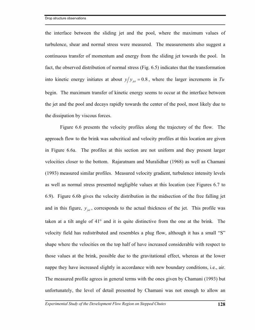
Drop structure observations
Experimental Study of the Development Flow Region on Stepped Chutes 128
the interface between the sliding jet and the pool, where the maximum values of
turbulence, shear and normal stress were measured. The measurements also suggest a
continuous transfer of momentum and energy from the sliding jet towards the pool. In
fact, the observed distribution of normal stress (Fig. 6.5) indicates that the transformation
into kinetic energy initiates at about 0.8jety y = , where the larger increments in Tu
begin. The maximum transfer of kinetic energy seems to occur at the interface between
the jet and the pool and decays rapidly towards the center of the pool, most likely due to
the dissipation by viscous forces.
Figure 6.6 presents the velocity profiles along the trajectory of the flow. The
approach flow to the brink was subcritical and velocity profiles at this location are given
in Figure 6.6a. The profiles at this section are not uniform and they present larger
velocities closer to the bottom. Rajaratnam and Muralidhar (1968) as well as Chamani
(1993) measured similar profiles. Measured velocity gradient, turbulence intensity levels
as well as normal stress presented negligible values at this location (see Figures 6.7 to
6.9). Figure 6.6b gives the velocity distribution in the midsection of the free falling jet
and in this figure, jety , corresponds to the actual thickness of the jet. This profile was
taken at a tilt angle of 41° and it is quite distinctive from the one at the brink. The
velocity field has redistributed and resembles a plug flow, although it has a small “S”
shape where the velocities on the top half of have increased considerable with respect to
those values at the brink, possible due to the gravitational effect, whereas at the lower
nappe they have increased slightly in accordance with new boundary conditions, i.e., air.
The measured profile agrees in general terms with the ones given by Chamani (1993) but
unfortunately, the level of detail presented by Chamani was not enough to allow an

Drop structure observations
Experimental Study of the Development Flow Region on Stepped Chutes 129
adequate comparison. Similar to the brink section, values of velocity gradient, turbulence
intensity and normal stress were negligible.
Velocity profiles in the sliding jet are given in Figure 6.5c. This figure presents
profiles at the intersection line and at the midsection of the sliding jet; they were taken at
tilt angles of 45° ( )0.489cy h = and 40° ( )0.779cy h = . The velocity profile at the
intersection line presents a more accentuated “S” shape with still larger velocity values
on the bottom section of the jet. Given the shape of the profile, it seems that the
gravitational effect together with the two air boundaries has its maximum influence at the
section. No effect of the recirculating pool is felt yet at this location. The transition of
the profile towards the pool is sharp and the values of velocity inside the pool get close to
zero quickly, this indicates the possibility of a stagnation zone in the vicinity of the
intersection between the free falling jet and the pool. On the other hand, the profiles at
the midsection of the sliding jet showed the interaction effects of the recirculating pool.
Lower velocities were measured on the bottom section of the jet while larger ones were
measured at the top, resembling a uniform velocity profile. This re-arrangement of the
velocity profile is likely to be caused by the strong interaction between the recirculating
pool and the jet. Moreover, this interaction developed velocities in the recirculating pool
and therefore there is a profile inside the pool, in which the decrease in velocity is less
abrupt. Chamani (1993) and Lin et al. (2002) measured similar profiles in the midsection
of a sliding jet. Magnitudes and profiles of velocity gradient, turbulence intensity and
normal stress were similar in both, intersection line and midsection, (Figure 6.7 to 6.9).
Finally, the velocity field at the toe of the sliding jet is giving in Figure 6.6d. The
shape is fairly uniform and they are in agreement with the profiles reported by

Drop structure observations
Experimental Study of the Development Flow Region on Stepped Chutes 130
Bakhmeteff and Feodoroff (1943). Measured turbulence intensities were smaller than
12% while normal stress values were smaller than 0.03; in both cases, the maximum
values occurred close to the bottom. Downstream of this location the flow was always
supercritical.
6.4 Local void fraction and chord lengths
Similar to velocity, the local void fraction was measured at the brink, as a free
falling jet, a sliding jet, and at the toe. Nevertheless, small values were measured at all
sections. Figure 6.10 shows the variation of the void fraction profile with depth. Two
things are noticeable form this figure. Firstly, the distribution of the local void fraction
has a similar shape for both discharges and secondly, larger void fractions were detected
inside the reciculating pool area where turbulence intensity levels where also larger.
Chord lengths distributions at the intersection line and at the midsection of the
sliding jet are presented in Figure 6.11. Inspection of this figure suggests that more
bubbles were detected in the intersection line than at the midsection. Furthermore, chord
sizes at the intersection line are smaller than at the midsection.

Drop structure observations
Experimental Study of the Development Flow Region on Stepped Chutes 131
a)
b)
Figure 6.1 Flow geometry at a drop structure. a) aerated step cavity; b)
non-aerated step cavity.

Drop structure observations
Experimental Study of the Development Flow Region on Stepped Chutes 132
0 0.2 0.4 0.6 0.8 1 1.2 1.4
0
0.2
0.4
0.6
0.8
1
1.2
1.4
1.6
1.8
2
U / Uavg
y / y
jet (f
rom
sur
face
)
(a)
yc / h = 0.489 yjet = 31 mm
yc / h = 0.779 yjet = 57 mm
0 0.2 0.4 0.6 0.8 1 1.2 1.4
0
0.2
0.4
0.6
0.8
1
1.2
1.4
1.6
1.8
2
U / Uavg
y / y
jet (f
rom
sur
face
)
(b)
yc / h = 0.489 yjet = 34 mm
yc / h = 0.779 yjet = 54 mm
0 0.2 0.4 0.6 0.8 1 1.2 1.4
0
0.2
0.4
0.6
0.8
1
1.2
1.4
1.6
1.8
2
U / Uavg
y / y
jet (f
rom
sur
face
)
(c)
Aerated yc / h = 0.489 yjet = 31 mm
Non-aerated yc / h = 0.489 yjet = 34 mm
0 0.2 0.4 0.6 0.8 1 1.2 1.4
0
0.2
0.4
0.6
0.8
1
1.2
1.4
1.6
1.8
2
U / Uavg
y / y
jet (f
rom
sur
face
)
(d)
Aerated yc / h = 0.779 yjet = 57 mm
Non-aerated yc / h = 0.779 yjet = 54 mm
Figure 6.2 Velocity profiles on the midsection of the sliding jet. a)
Aerated flow; b) fully depleted nappe; c) low discharge, d) large
discharge.

Drop structure observations
Experimental Study of the Development Flow Region on Stepped Chutes 133
-50 0 50 100 150 200 250 300 350 400 450
0
0.2
0.4
0.6
0.8
1
1.2
1.4
1.6
1.8
2
dU / dy (m/s/m)
y / y
jet (f
rom
sur
face
)
(a)
yc / h = 0.489 yjet = 31 mm
yc / h = 0.779 yjet = 57 mm
-50 0 50 100 150 200 250 300 350 400 450
0
0.2
0.4
0.6
0.8
1
1.2
1.4
1.6
1.8
2
dU / dy (m/s/m)
y / y
jet (f
rom
sur
face
)
(b)
yc / h = 0.489 yjet = 34 mm
yc / h = 0.779 yjet = 54 mm
-50 0 50 100 150 200 250 300 350 400 450
0
0.2
0.4
0.6
0.8
1
1.2
1.4
1.6
1.8
2
dU / dy (m/s/m)
y / y
jet (f
rom
sur
face
)
(c)
Aerated yc / h = 0.489 yjet = 31 mm
Non-aerated yc / h = 0.489 yjet = 34 mm
-50 0 50 100 150 200 250 300 350 400 450
0
0.2
0.4
0.6
0.8
1
1.2
1.4
1.6
1.8
2
dU / dy (m/s/m)
y / y
jet (f
rom
sur
face
)
(d)
Aerated yc / h = 0.779 yjet = 57 mm
Non-aerated yc / h = 0.779 yjet = 54 mm
Figure 6.3 Velocity gradient profiles on the midsection of the sliding jet.
a) Aerated flow; b) fully depleted nappe; c) low discharge, d) large
discharge.
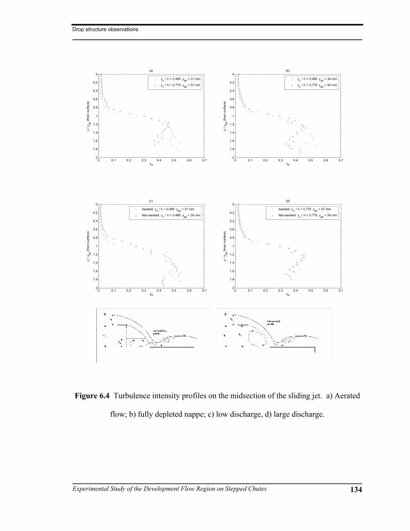
Drop structure observations
Experimental Study of the Development Flow Region on Stepped Chutes 134
0 0.1 0.2 0.3 0.4 0.5 0.6 0.7
0
0.2
0.4
0.6
0.8
1
1.2
1.4
1.6
1.8
2
Tu
y / y
jet (f
rom
sur
face
)
(a)
yc / h = 0.489 yjet = 31 mm
yc / h = 0.779 yjet = 57 mm
0 0.1 0.2 0.3 0.4 0.5 0.6 0.7
0
0.2
0.4
0.6
0.8
1
1.2
1.4
1.6
1.8
2
Tu
y / y
jet (f
rom
sur
face
)
(b)
yc / h = 0.489 yjet = 34 mm
yc / h = 0.779 yjet = 54 mm
0 0.1 0.2 0.3 0.4 0.5 0.6 0.7
0
0.2
0.4
0.6
0.8
1
1.2
1.4
1.6
1.8
2
Tu
y / y
jet (f
rom
sur
face
)
(c)
Aerated yc / h = 0.489 yjet = 31 mm
Non-aerated yc / h = 0.489 yjet = 34 mm
0 0.1 0.2 0.3 0.4 0.5 0.6 0.7
0
0.2
0.4
0.6
0.8
1
1.2
1.4
1.6
1.8
2
Tu
y / y
jet (f
rom
sur
face
)
(d)
Aerated yc / h = 0.779 yjet = 57 mm
Non-aerated yc / h = 0.779 yjet = 54 mm
Figure 6.4 Turbulence intensity profiles on the midsection of the sliding jet. a) Aerated
flow; b) fully depleted nappe; c) low discharge, d) large discharge.

Drop structure observations
Experimental Study of the Development Flow Region on Stepped Chutes 135
0 0.05 0.1 0.15 0.2 0.25 0.3 0.35 0.4 0.45
0
0.2
0.4
0.6
0.8
1
1.2
1.4
1.6
1.8
2
u2 ( m2/s2 )
y / y
jet (f
rom
sur
face
)
(a)
yc / h = 0.489 yjet = 31 mm
yc / h = 0.779 yjet = 57 mm
0 0.05 0.1 0.15 0.2 0.25 0.3 0.35 0.4 0.45
0
0.2
0.4
0.6
0.8
1
1.2
1.4
1.6
1.8
2
u2 ( m2/s2 )
y / y
jet (f
rom
sur
face
)
(b)
yc / h = 0.489 yjet = 34 mm
yc / h = 0.779 yjet = 54 mm
0 0.05 0.1 0.15 0.2 0.25 0.3 0.35 0.4 0.45
0
0.2
0.4
0.6
0.8
1
1.2
1.4
1.6
1.8
2
u2 ( m2/s2 )
y / y
jet (f
rom
sur
face
)
(c)
Aerated yc / h = 0.489 yjet = 31 mm
Non-aerated yc / h = 0.489 yjet = 34 mm
0 0.05 0.1 0.15 0.2 0.25 0.3 0.35 0.4 0.45
0
0.2
0.4
0.6
0.8
1
1.2
1.4
1.6
1.8
2
u2 ( m2/s2 )
y / y
jet (f
rom
sur
face
)
(d)
Aerated yc / h = 0.779 yjet = 57 mm
Non-aerated yc / h = 0.779 yjet = 54 mm
Figure 6.5 Normal stress profiles on the midsection of sliding jet. a) Aerated flow; b)
fully depleted nappe; c) low discharge, d) large discharge.

Drop structure observations
Experimental Study of the Development Flow Region on Stepped Chutes 136
0 0.2 0.4 0.6 0.8 1 1.2 1.4
0
0.1
0.2
0.3
0.4
0.5
0.6
0.7
0.8
0.9
1
U / Uavg
y / y
T (fro
m s
urfa
ce)
(a)
yc / h = 0.489 yT = 49 mm
yc / h = 0.779 yT = 78 mm
0 0.2 0.4 0.6 0.8 1 1.2 1.4
0
0.1
0.2
0.3
0.4
0.5
0.6
0.7
0.8
0.9
1
U / Uavg
y / y
jet (
from
upp
er n
appe
)
(b)
yc / h = 0.489 yjet = 37 mm
0 0.2 0.4 0.6 0.8 1 1.2 1.4
0
0.2
0.4
0.6
0.8
1
1.2
1.4
1.6
1.8
2
U / Uavg
y / y
jet (f
rom
sur
face
)
(c)
Midsection yc / h = 0.489 yjet = 31 mm
Intersection yc / h = 0.779 yjet = 60 mm
Midsection yc / h = 0.779 yjet = 57 mm
0 0.2 0.4 0.6 0.8 1 1.2 1.4
0
0.1
0.2
0.3
0.4
0.5
0.6
0.7
0.8
0.9
1
U / Uavg
y / y
T (fro
m s
urfa
ce)
(d)
yc / h = 0.489 yT = 29 mm
yc / h = 0.779 yT = 52 mm
Figure 6.6 Velocity profiles along the jet trajectory. a) upstream brink;
b) free falling jet; c) sliding jet, d) toe of sliding jet.

Drop structure observations
Experimental Study of the Development Flow Region on Stepped Chutes 137
-50 0 50 100 150 200 250 300 350 400 450
0
0.1
0.2
0.3
0.4
0.5
0.6
0.7
0.8
0.9
1
dU / dy (m/s/m)
y / y
T (fro
m s
urfa
ce)
(a)
yc / h = 0.489 yT = 49 mm
yc / h = 0.779 yT = 78 mm
-50 0 50 100 150 200 250 300 350 400 450
0
0.1
0.2
0.3
0.4
0.5
0.6
0.7
0.8
0.9
1
dU / dy (m/s/m)
y / y
jet (f
rom
sur
face
)
(b)
yc / h = 0.489 yjet = 37 mm
-50 0 50 100 150 200 250 300 350 400 450
0
0.2
0.4
0.6
0.8
1
1.2
1.4
1.6
1.8
2
dU / dy (m/s/m)
y / y
jet (f
rom
sur
face
)
(c)
Midsection yc / h = 0.489 yjet = 31 mm
Intersection yc / h = 0.779 yjet = 60 mm
Midsection yc / h = 0.779 yjet = 57 mm
-50 0 50 100 150 200 250 300 350 400 450
0
0.1
0.2
0.3
0.4
0.5
0.6
0.7
0.8
0.9
1
dU / dy (m/s/m)
y / y
T (fro
m s
urfa
ce)
(d)
yc / h = 0.489 yT = 29 mm
yc / h = 0.779 yT = 52 mm
Figure 6.7 Velocity gradient profiles along the jet trajectory. a) upstream
brink; b) free falling jet; c) sliding jet, d) toe of sliding jet.
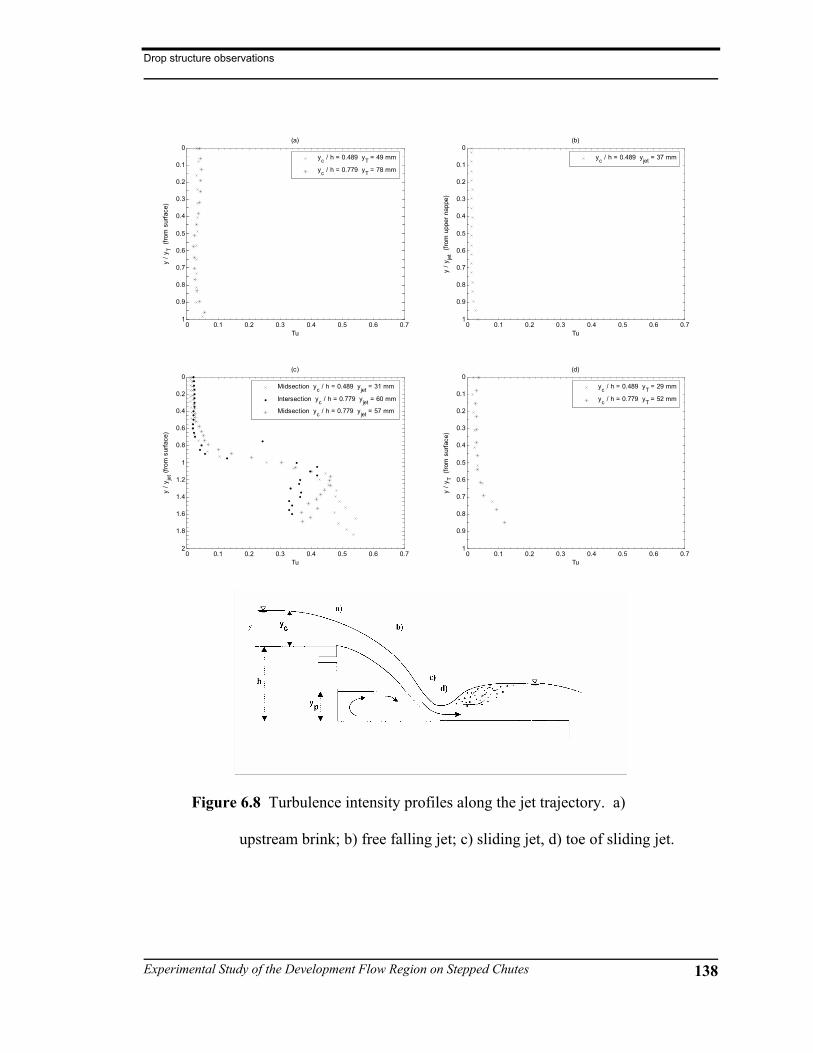
Drop structure observations
Experimental Study of the Development Flow Region on Stepped Chutes 138
0 0.1 0.2 0.3 0.4 0.5 0.6 0.7
0
0.1
0.2
0.3
0.4
0.5
0.6
0.7
0.8
0.9
1
Tu
y / y
T (fro
m s
urfa
ce)
(a)
yc / h = 0.489 yT = 49 mm
yc / h = 0.779 yT = 78 mm
0 0.1 0.2 0.3 0.4 0.5 0.6 0.7
0
0.1
0.2
0.3
0.4
0.5
0.6
0.7
0.8
0.9
1
Tu
y / y
jet (
from
upp
er n
appe
)
(b)
yc / h = 0.489 yjet = 37 mm
0 0.1 0.2 0.3 0.4 0.5 0.6 0.7
0
0.2
0.4
0.6
0.8
1
1.2
1.4
1.6
1.8
2
Tu
y / y
jet (f
rom
sur
face
)
(c)
Midsection yc / h = 0.489 yjet = 31 mm
Intersection yc / h = 0.779 yjet = 60 mm
Midsection yc / h = 0.779 yjet = 57 mm
0 0.1 0.2 0.3 0.4 0.5 0.6 0.7
0
0.1
0.2
0.3
0.4
0.5
0.6
0.7
0.8
0.9
1
Tu
y / y
T (fro
m s
urfa
ce)
(d)
yc / h = 0.489 yT = 29 mm
yc / h = 0.779 yT = 52 mm
Figure 6.8 Turbulence intensity profiles along the jet trajectory. a)
upstream brink; b) free falling jet; c) sliding jet, d) toe of sliding jet.

Drop structure observations
Experimental Study of the Development Flow Region on Stepped Chutes 139
0 0.05 0.1 0.15 0.2 0.25 0.3 0.35 0.4 0.45
0
0.1
0.2
0.3
0.4
0.5
0.6
0.7
0.8
0.9
1
u2 (m2 / s2)
y / y
T (fro
m s
urfa
ce)
(a)
yc / h = 0.489 yT = 49 mm
yc / h = 0.779 yT = 78 mm
0 0.05 0.1 0.15 0.2 0.25 0.3 0.35 0.4 0.45
0
0.1
0.2
0.3
0.4
0.5
0.6
0.7
0.8
0.9
1
u2 (m2 / s2)
y / y
jet (
from
upp
er n
appe
)
(b)
yc / h = 0.489 yjet = 37 mm
0 0.05 0.1 0.15 0.2 0.25 0.3 0.35 0.4 0.45
0
0.1
0.2
0.3
0.4
0.5
0.6
0.7
0.8
0.9
u2 (m2 / s2)
y / y
jet (f
rom
sur
face
)
(c)
Midsection yc / h = 0.489 yjet = 31 mm
Intersection yc / h = 0.779 yjet = 60 mm
Midsection yc / h = 0.779 yjet = 57 mm
0 0.05 0.1 0.15 0.2 0.25 0.3 0.35 0.4 0.45
0
0.1
0.2
0.3
0.4
0.5
0.6
0.7
0.8
0.9
1
u2 (m2 / s2)
y / y
T (fro
m s
urfa
ce)
(d)
yc / h = 0.489 yT = 29 mm
yc / h = 0.779 yT = 52 mm
Figure 6.9 Normal stress profiles along the jet trajectory. a) upstream
brink; b) free falling jet; c) sliding jet, d) toe of sliding jet.
Drop structure observations
Experimental Study of the Development Flow Region on Stepped Chutes 140
0 0.001 0.002 0.003 0.004 0.005 0.006 0.007 0.008 0.009 0.01
0
0.2
0.4
0.6
0.8
1
1.2
1.4
1.6
1.8
2
Local void fraction
y / y
jet (f
rom
sur
face
)
(a)
yc / h = 0.489 yjet = 31 mm
yc / h = 0.779 yjet = 57 mm
Figure 6.10 Local void fraction. a) midsection of sliding
jet.

Drop structure observations
Experimental Study of the Development Flow Region on Stepped Chutes 141
0 5 10 15 20 25 300
0.02
0.04
0.06
0.08
0.1
0.12
0.14
0.16
0.18(a)
Chord length (mm)
Rel
ativ
e fre
quen
cy
Aerated
yc / h = 0.489
Bubbles = 176
Mean length = 19 mm
0 2 4 6 8 10 12 14 160
0.05
0.1
0.15
0.2
0.25(b)
Chord length (mm)
Rel
ativ
e fre
quen
cy
Aerated
yc / h = 0.779
Bubbles = 1396
Mean length = 7.9 mm
0 5 10 15 20 250
0.02
0.04
0.06
0.08
0.1
0.12
0.14(c)
Chord length (mm)
Rel
ativ
e fre
quen
cy
Aerated
yc / h = 0.779
Bubbles = 635
Mean length = 13 mm
Figure 6.11 Chord length distribution at midsection (a and
c) and intersection line (b) of the sliding jet.
Summary and conclusions
Experimental Study of the Development Flow Region on Stepped Chutes 142
Chapter 7 Summary and conclusions
7.1 Introduction
In this study a constant temperature anemometer as well as pressure transducers
were used to experimentally study the characteristics of the flow development region on
stepped chutes. Three physical models with chute slopes of 3.5 :1H V , 5 :1H V ,
10 :1H V were used in the study; all models had five steps 15 cm in height. Several flow
conditions in the range of 0.47 1.66cy h≤ ≤ were tested in conjunction with aerated and
non-aerated step cavities.
7.2 Summary
Constant temperature anemometry
The constant temperature anemometry system used in this study was subject to
three problems: probe contamination, bubble formation, and temperature drift. These
problems, which are commonly attributed to the use of CTA in water flow measurements,

Summary and conclusions
Experimental Study of the Development Flow Region on Stepped Chutes 143
can be overcome by an appropriate selection of the overheat ratio, careful application of a
suitable temperature compensation technique and frequent calibrations.
The experimental results indicated that the constant sensor temperature technique
can be used to adequately compensate temperature drift as long as the water temperature
variations are smaller than 0.5 C° . In using this technique, the compensation should be
applied to the CTA raw data where the functional form of the compensation depends on
the overheat ratio and the flow velocity. In this study, a linear correction in terms of Nu
and Θ was obtained for each fixed value of flow velocity. In addition to this, heat
transfer relationships for the expected water temperature range should be obtained for
each CTA setup condition.
On the other hand, compensation of temperature drift by means of a constant
overheat ratio technique produced good results and does not require numerous
calibrations. This procedure should be preferred over a constant sensor temperature
when dealing with water flows. In this study, manual compensation of the overheat ratio
produced good results, but it required a post-processing analysis of the raw data in order
to correct for possible under/over compensation. This correction was successfully
applied in this study but an automatic compensation should be developed in order to
eliminate this step. Moreover, from the analytical functions tested to represent the heat
transfer relationship on the constant overheat ratio technique; the extended power law (Eq.
3.4) produced the best representation of the conical hot-film probe response. A fourth-
order polynomial in terms of E as well as a cubic spline interpolation produced
satisfactory results as well. Nevertheless, these two methods pose a risk of strong
deviations for the lower range of flow velocities.
Summary and conclusions
Experimental Study of the Development Flow Region on Stepped Chutes 144
In dealing with air-water flows, the phase detection methodology is quite sensitive
to the selection of the threshold values. In this study several approaches to select those
values were attempted. The autocorrelation values of the empirical cumulative density
function produced an adequate estimation of such values in terms of CTA output voltage.
In the case of the slope threshold method, the change of sign of the CTA signal slope
produced the best results in identifying the characteristic points of a bubble.
Constant temperature anemometry has the potential to become as valuable tool in
the study of water flow problems as it is in air flows. The technique has good spatial and
temporal resolution and it is capable of handling two phase flow. Its use at large
hydraulic facilities should not be overlooked since current hot-film systems are capable
of overcoming the issues that prevented their use in water flows previously.
Velocity and local void fraction observations
The experimental observations indicated that the conditions along the
development flow region on stepped chutes are complex and change abruptly between
steps. As an overall, supercritical flow was observed along the steps and provision of air
into the step cavity affected the first step only. In fact, the flow geometry of this step
depended on whether or not air was supplied. In this regard the first step resembled the
flow behavior of a drop structure. This was not observed on the remaining steps
It was observed that the flow jet breaks up easily on steeper slopes, this is because
shorter step treads do not provide enough distance for the flow to dissipate the
perturbations produce by the impact onto the step. Hence, two-phase flow along the
chute is obtained at smaller discharges for steep chutes than for mild ones. Furthermore,

Summary and conclusions
Experimental Study of the Development Flow Region on Stepped Chutes 145
measurements indicate that the condition of the step cavity does not affect the velocity
field at the step brinks. This field presents a logarithmic distribution as found in an open
channel. However, it vanishes quickly as the jet break up process develops. Before this
occurred in each of the models, a similar velocity distribution was observed at the step
brinks. It was also observed that on the transition flow regime an air cavity randomly
formed on some of the steps. The formation process of this cavity looked like a “bursting
mechanism” where air bubbles spontaneously appear and flock to form the cavity. This
phenomenon will bring complications if an attempt to mathematically model the
transition flow is carried out. This “bursting mechanism” would require the switch on
and off of a boundary condition on the lower nappe of the jet.
In regards to the air pocket condition, it was observed that in aerated flows, the
recirculating pool became shallower and elongated in the downstream direction. If the
step cavity is full of water (non-aerated condition), two symmetric spiral vortices were
observed in the vicinity of the step riser, these vortices had a flow direction towards the
sides of the models in the area closest to the riser and an ascending flow direction.
Additionally, it was observed that the length of the step cavity was about 2 to 3h . In
transition flow regime, the step cavity was usually full air bubbles and high levels of
turbulence were observed. If a stepped chute with horizontal steps would be used as a
fish ladder, fishes would be forced to rest in the step cavity before continuing their
upstream journey. However, given the observed size of the cavity it is unlikely that
mature fishes would fit into it. Furthermore, the high turbulence levels together with the
observed vortices do not provide good conditions for resting while the large quantities of
air bubbles might locally saturate the water with oxygen or nitrogen, a harmful condition

Summary and conclusions
Experimental Study of the Development Flow Region on Stepped Chutes 146
for fish. On the other hand, the mixing of chemical with the water could be carried out
on this location since the vortices will produce enough agitation for their dispersion and
possible reaction with air.
According to the measurements, the local void fraction along the chute is not
affected by the condition of the step cavity. In fact, the air concentration distribution
throughout the flow development region seems to have a “C” shape. Larger values were
observed at the bottom and top of the flow while minimum values in the middle of the
water column. The observations suggest that the local void fraction remains below 0.6.
Moreover, larger chord sizes were measured immediately downstream of the jet impact
than on the step brinks. In addition, larger chord sizes were measured on the steeper
slopes. Knowledge of these parameters is of vital importance for the proper design of
stepped chutes as water treatment systems since they allow the quantification of the air-
water interface area. Moreover, they also facilitate the assessment of the gas transfer
between air and water. Consequently, the environmental effects of the induced two phase
flow on the downstream ecosystem can be effectively assessed.
Finally, the water surface profile was observed to be in phase with the chute
geometry within the clear water region. Additionally, a significant amount of spray was
observed on the transition flow regime and drops were observed to reach 4 to 5h above
the chute invert on average. Nevertheless, some drops were observed up to 7 to 8h .
This is of considerable importance when designing side wall heights, especially in cold
climates where icy conditions in the vicinity of the structure are potentially dangerous. It
is also important to mention that surface shock waves were observed in Model III during
the skimming flow regime, and in some degree, they were also present on Model II

Summary and conclusions
Experimental Study of the Development Flow Region on Stepped Chutes 147
Shock waves were not observed on Model I probably because the relatively step slope
prevented their formation. The shock waves produce considerable disturbance on the
water surface, especially after the second step, they also entrain air into the upper layers
of the water stream. The observed shock waves reached heights of about 1 to 2h over
the pseudo bottom, factor that should be considered during the dimensioning of the side
walls.
Pressure observations
Pressure observations carried out in this study indicate that the value of cy h at
which step cavities become filled with water seems to have a dependency on the chute
slope. In fact, the cavity condition (aerated or non-aerated) plays a role on the first step
only. In addition, on the three slopes studied, the fourth steps did not become filled with
water at the same discharge, but rather in a progressive order, which is an indication that
the preceding upstream flow condition significantly affects the behavior of each step.
The pressure observations also indicated that the step cavity pressure behaves differently
on each step.
As observed, the occurrence of minimum pressure values agrees with the regime
boundaries of a long stepped spillway, however, the value of cy h at which the
minimum value occurs increases in the downstream direction, from the first sub-regime
of the transition regime to the second sub-regime. Measurements indicate that pressure
distribution along a tread is different on each step, although they share the presence of a
peak value at the point of flow impact. Additionally, observations on the different chute
slopes indicate that there is no ‘typical’ pressure profile on the treads, where each model

Summary and conclusions
Experimental Study of the Development Flow Region on Stepped Chutes 148
seems to behave in a characteristic way with some similarities but not sufficient to
determine a unique pressure profile. Regarding the step risers, measurements within a
model displayed a similar pressure profile for the aerated and non-aerated conditions.
Nevertheless, the pressure profiles on each step are not similar. On the vertical face, a
gradual modification of the pressure distribution was observed as air gets entrained in the
flow.
Finally, no correlation was observed on the recirculation pool depth in any of the
steps or between them. The expressions for pool depth of drop structures do not
represent the observed depths. Moreover, the water level in the pool fluctuated
intensively in a wavy pattern. This wavy level was more intense for the steeper slopes
and it was also observed that on average, the water level was slightly inclined towards the
point of jet impact.
Drop structure observations
Taking advantage of the geometric similarity between a drop structure and the
first step of a stepped chute, several measurements were carried out on Model II in order
to study such a structure. These observations indicated that in the sliding jet there is no
significant difference between the aerated and non-aerated cavities. In addition, the
experimental results confirmed the presence of a uniform velocity distribution in the
sliding jet and a quantification of the shear layer between the jet and the pool was
successfully achieved. Finally, the measurements indicated that the transfer of kinetic
energy from the jet to the pool –as turbulence- and subsequent dissipation by viscous
forces seems to govern the observed energy losses.

Summary and conclusions
Experimental Study of the Development Flow Region on Stepped Chutes 149
7.3 Conclusions
The following conclusions can be drawn from this study:
i. The use of constant temperature anemometry in water flows should not be
overlooked. The constant overheat ratio procedure produced good results and it is
a strong technique for dealing with the non-isothermal conditions often
encountered at hydraulic laboratories.
ii. Conical hot-film probes proved to be a valuable tool in this study not only due to
its great spatial and temporal resolution but also due to its capability to cope with
the problem of the two-phase flow.
iii. The use of the autocorrelation of the empirical cumulative density function proof
to be a good procedure to estimate the amplitude threshold allowing the
separation of the two phases. In addition, the change on sign of the slope signal
was the selected value to identify the bubble characteristic points.
iv. In the development flow region of stepped chutes the conditions are complex and
they change abruptly between steps. These abrupt changes are chiefly due to the
disintegration of the jet.
v. Flow conditions along the chutes do not resemble a drop structure. Furthermore,
provision of air into the step cavity affects the flow geometry of the first step only.
vi. A logarithmic velocity distribution was observed in the flow downstream of the
jet impact. However, this distribution vanishes quickly as the break up of the jet
takes place.
Summary and conclusions
Experimental Study of the Development Flow Region on Stepped Chutes 150
vii. Observations of the filling up process in a step cavity indicated that the preceding
upstream flow condition have a significant affect on the behavior of each step.
viii. The boundary between regimes seems to coincide with local minimum pressure
values in the step cavity.
ix. A “bursting mechanism” was observed on the step cavity during the transition
flow regime. This mechanism allows the air cavity to form in a random fashion
bringing complexity on a possible mathematical model of these structures.
x. Shock waves developed at skimming flow regime on chutes with mild slopes.
This is an important phenomenon since it has considerable design implications.
At the stepper slope, i.e. Model I, shock waves were not observed.
xi. In the recirculating pool, depths fluctuate intensely and the shape of the pool
seems to become shallower and elongated in the downstream direction.
xii. If the step cavity was full of water, the recirculating pool was small. This fact
could preclude the use of stepped chutes as fish passage since a mature fish may
not fit into the possible resting area: the step cavity. Furthermore, the presence of
vortices and large quantities of air bubbles are also detrimental conditions for this
possible use.
xiii. The quantification of the local void fractions, chord length and turbulence levels
provide environmental engineers valuable information for the design of stepped
chutes as water treatment systems. Similarly, they allow the correct assessment of
the gases transfer between the air and water when dealing with stepped chutes.
Assessment that benefits the quantification of effects on the downstream aquatic
ecosystem.

Summary and conclusions
Experimental Study of the Development Flow Region on Stepped Chutes 151
xiv. Observations indicated that there is no ‘typical’ pressure profile on either the tread
or the step risers.
xv. A qualitative and quantitative description of the shear layer between the jet and
pool was successfully achieved.
7.4 Future works
The use of constant temperature anemometry has proven to be a useful tool at a
large hydraulic facility. In spite of the fact that CTA has been around for more than 30
years, automatic temperature compensation for water flows is not as developed as it is for
air flows. The successful implementation of such a technique in a water flow still
requires the development of an adequate probe. The desirable probe should be fast
enough to cope with the frequency response of current conical hot-film probes,
insensitive to all flow parameters but water temperature, and small enough so that it does
not affect the flow. In this way, a temperature compensator bridge could be used instead
of a standard bridge.
Many aspects of stepped chutes and the flow characteristics are still unfamiliar to
researchers and practitioners. The vast field of inclined and pooled steps have not been
studied yet. Nevertheless, these should be studied in detail especially since they may
provide suitable fish passing structures. In addition, the environmental applications of
stepped chutes are quite varied and therefore, studies for specific applications will always
be needed.
This study provided valuable insight to the development flow region of stepped
chutes. Nevertheless, the flow in this region is complex and more analysis of the velocity
Summary and conclusions
Experimental Study of the Development Flow Region on Stepped Chutes 152
field and void fraction distribution should be carried out. Specific studies on the 3-
dimensional flow observed inside the recirculating pool should be performed. It is likely
that this circulation pattern and the presence of shock waves are linked and should be
studied in detail. In addition, the presence of such a wave is a problem that should
addressed since they may significantly affect the performance of the structure. It also
important to carried out a systematic study on the effect that model width could have on
the formation of shock waves. Moreover, the length of the development flow region on
mild slopes remains to be determined and the mechanism of the air cavity formation on
transition flow regime deserves special attention.
This study also encountered unexpected pressure profiles in the development flow
region. These profiles presented a saw shape, which are not typical, and therefore they
need to be studied in detail in order to be confirmed. Furthermore, this research
suggested a change in the hydraulic behavior of stepped chutes when the slope changes
from 5.7° to 11.3° . The occurrence of this phenomenon should also be addressed in the
future.

References
Experimental Study of the Development Flow Region on Stepped Chutes 153
References
Agha, M. and Ibrahim, M.T. (1984). “Algorithm AS 203: maximum likelihood
estimation of mixtures of distributions”. Applied Statistics, 33(3), 327-332.
Aigner, D. (2001). “Hydraulic design of pooled step cascades”. 21st Century: The
new era for hydraulic research and its applications. Proc. 29th IAHR Congress,
Theme D, Vol. I., G. Li, ed., Beijing, China, 635-640.
Bakhmeteff, B.A. and Feodoroff, N.V. (1943). “Discussion of Moore (1943)”.
Transactions, ASCE, Vol. 108, 1364-1373.
Boes, R.M. (1999). “Physical model study on two-phase cascade flow”. Proc. 28th
IAHR Congress. Graz, Austria. CD-rom.
Boes, R.M. (2000). “Scale effects in modeling two-phase spillway flow”. Intl.
Workshop on Hydraulics of stepped spillways, H.E. Minor and W.H. Hager, eds.,
Balkema Publ., Netherlands, 53-60.
Boes, R.M. and Minor, H.E. (2000). “Guidelines for the hydraulic design of
stepped spillways”. Intl. Workshop on Hydraulics of stepped spillways, H.E.
Minor and W.H. Hager, eds., Balkema Publ., Netherlands, 163-170.
Bruun, H.H. (1996). “Hot-film anemometry in liquid flows”. Meas. Sci. Technol.,

References
Experimental Study of the Development Flow Region on Stepped Chutes 154
7(10), 1301-1312.
Bruun, H.H.; Khan, M.A.; Al-Kayiem, H.H. and Fardad, A.A. (1988). “Velocity
calibration relationships for hot-wire anemometry”. J. Phys. E: Sci. Instrum., the
Institute of Physics, 21, 225-232.
Chamani, M.R. (1993). “Jet flow on stepped spillways and drops”. M.Sc. thesis,
University of Alberta, Alberta, Canada.
Chamani, M.R. (1997). “Skimming flow in a large model of a stepped spillway”.
Ph.D. thesis, University of Alberta, Canada.
Chamani, M.R. and Rajaratnam, N. (1999). “Onset of skimming flow on stepped
spillways”. J. Hydr. Engrg., ASCE, 125(9), 969-971. Discussion: 127(6), 519-
525.
Chanson, H. (1994). “Hydraulics of nappe flow regime above stepped chutes and
spillways”. Aust. Civil Eng. Trans., IEAust., CE36(1), 69-76.
Chanson, H. (1995a). Hydraulic design of stepped cascades, channels, weirs and
spillways. Pergamon. Oxford, U.K.
Chanson, H. (1995b). “History of stepped channels and spillways: a rediscovery of
the “wheel”’. Can. J. of Civil Eng., 22(2), 247-259.
Chanson, H. (1996). “Prediction of the transition nappe/skimming flow on a
stepped channel”. J. Hydr. Res., IAHR, 34(3), 421-429.
Chanson, H. (1998). “Le développement historique des cascades et fontaines en
gradins” (Historical development of stepped cascades and fountains). La Houille
blanche, Revue de la Société Hydrotechnique de France, No 7, 76-84. (In
French).

References
Experimental Study of the Development Flow Region on Stepped Chutes 155
Chanson, H. (1999). “Current expertise and experience on stepped chute flows”.
Seminar presented at Kyoto University, Disaster Prevention Research Institute.
April, Kyoto, Japan.
Chanson, H. (2000a). “Hydraulics of Roman Aqueducts : Steep Chutes, Cascades
and Dropshafts”. American J. of Archaeology, 104(1), 47-72.
Chanson, H. (2001a). “A transition flow regime on stepped spillway? The facts”.
21st Century: The new era for hydraulic research and its applications. Proc. 29th
IAHR Congress, Theme D, Vol. I., G. Li, ed., Beijing, China, 490-498.
Chanson, H. (2001b). Caractéristiques diphasiques des ecoulements sur les coursiers en
marches d’escalier. ). La Houille blanche, Revue de la Société Hydrotechnique
de France, No 8, 16-28. (In French).
Chanson, H. (2001c). The hydraulics of stepped chutes and spillways.. Balkema. Lisse,
The Netherlands.
Chanson, H. and Toombes, L. (1998a). “Air-water flow structures at an abrupt
drop with supercritical flow”. Proc. 3rd Intl. Conf. Multiphase flow, ICMF’98,
Lyon, France, Session 2.2.5, Paper No. 119, 6 pages.
Chanson, H. and Toombes, L. (1998b). “Supercritical flow at an abrupt drop: flow
patterns and aeration”. Can. J. of Civil Eng., 25(5), 956-966.
Chanson, H. and Toombes, L. (2001). “Experimental investigation of air
entrainment in transition and skimming flows down a stepped chute. Application
to embankment overflow stepped spillways”, Report CE 158, University of
Queensland, Australia.
Chanson, H. and Toombes, L. (2004). “Hydraulics of stepped chutes: the transition

References
Experimental Study of the Development Flow Region on Stepped Chutes 156
flow”. J. Hydr. Res., IAHR, 42(1), 43-54.
Collins, D.C., and Williams, M.J. (1959). “Two-dimensional convection from heated
wires at low Reynolds numbers”. J. Fluid Mech., 6(3), 357-384.
Dantec Dynamics (2003). “Probes for Hot-wire Anemometry”. Publication No
103-105-07, Dantec Dynamics A/S, Denmark.
Dantec Dynamics (2005). “Technical data for conical film sensors”. Single sensor film
probes, conical film probes, <http://www.dantecmt.com> (Aug 3, 2005).
Delhaye, J.M. (1968). “Hot-film anemometry in two-phase flow”. Proc. 11th National
Heat transfer conferences, ASME/AIChE, Minneapolis, Minnesota, USA.
De Marinis, G., Fratino, U. and Piccinni, A.F. (2001). “Flow regimes on stepped
spillways”. 21st Century: The new era for hydraulic research and its
applications. Proc. 29th IAHR Congress, Theme D, Vol. I., G. Li, ed., Beijing,
China, 641-646.
Diez-Cascon, J., Blanco, J.L., Revilla, J. and Garcia, R. (1991). “Studies on the
hydraulic behaviour of stepped spillways”. Water Power & Dam Construction,
43(9), 22-26.
DISA. (1977). Instruction manual, DISA 55M system with 55M10 CTA standard bridge.
Disa Elektronik A/S, Denmark.
El-Kamash, M.K., Lowen, M.R. and Rajaratnam, M. (2005). “En experimental
investigation of jet flow on a stepped chute”. J. Hydr. Res., IAHR, 43(1), 31-43.
Essery, I.T.S., and Horner, M.W. (1978). “The hydraulic design of stepped
spillways”. Report No. 33, CIRIA, London, U.K.
Farrar, B. and Bruun, H.H. (1989). “Interaction effects between a cylindrical hot-film

References
Experimental Study of the Development Flow Region on Stepped Chutes 157
anemometer probe and bubbles in air/water and oil/water flows”. J. Phys. E: Sci.
Instrum., the Institute of Physics, 22, 114-123.
Farrar, B., Samways, A.L. Ali, J. and Bruun, H.H. (1995). “A computer-based hot-film
technique for two-phase flow measurements”. Meas. Sci. Technol., 6(10), 1528-
1537.
Hager, W. and Boes, R. (2000). “Backwater and drawdown curves in stepped
spillways”. Intl Workshop on Hydraulics of stepped spillways, H.E. Minor and
W.H. Hager, eds., Balkema Publ., Netherlands, 129-136.
Horner, M.W. (1969). “An analysis of flow on cascades of steps”. Ph.D. Thesis,
University of Birmingham, United Kingdom.
Houston, K.L. and Richardson, A.T. (1988). “Energy dissipation characteristics of a
stepped spillway for an RCC dam”. Proc. Intl. Symp. on hydraulics for high
dams, IAHR, Beijing, China, 91-98.
James, C., Comnino, M. and Palmer, M.W. (1999). “Effects of slope and step size on
the hydraulics of stepped chutes”. J. South African Inst. Civil Engrg., 41(2), 1-6.
Jørgensen, F.E. (2002). How to measure turbulence with hot-wire anemometers –a
Practical Guide, Dantec Dynamics A/S, Denmark.
Lekakis, I. (1996). “Calibration and signal interpretation for single and multiple
hot-wire/hot-film probes”. Meas. Sci. Technol., 7(10), 1313-1332.
Lilliefors, H.W. (1967). “On the Kolmogorv-Smirnov test for normality with mean and
variance unknown”. J. American Statistical Association, 62(318), 399-402.
Lin, C.; Huang, W.Y.; Suen, H.F.; Hsieh, S.C. (2002). “Study on the characteristics of velocity
field of free overfalls over a vertical drop”. Hydraulic Measurements and Experimental
Methods 2002, ASCE, U.S.A., 178-187.

References
Experimental Study of the Development Flow Region on Stepped Chutes 158
Macaitis, B. (1990). “Sidestream elevated pool aeration station design”. Proc. 2nd
Symp. On Gas transfer at water surfaces, air-water mass transfer, S.C. Wilhelms
and J.S. Gulliver, eds., ASCE, U.S.A., 670-681.
Minor, H.E., and Boes, R.M. (2001). “Hydraulic design of stepped spillways”. 21st
Century: The new era for hydraulic research and its applications. Proc. 29th
IAHR Congress, Theme D, Vol. I., G. Li, ed., Beijing, China, 754-759.
Minor, H.E. and Hager, W.H. (2000). Proceedings of the Intl. Workshop on
Hydraulics of stepped spillways. Zurich, Switzerland. Balkema Publ.,
Netherlands.
Ohtsu, I. and Yasuda, Y. (1997). “Characteristics of flow conditions on stepped
channels”. Energy and water: sustainable development. Proc. 27th IAHR
Congress, J.S. Gulliever and P.L. Viollet, eds., San Francisco, USA, 583-588.
Ohtsu, I.; Yasuda, Y. and Takahashi, M. (2004). “Flow characteristics of skimming
flows in stepped channels”. J. Hydr. Eng., ASCE, 130(9), 860-869.
Peyras, L.; Royet, P. and Degoutte, G. (1991). “Ecoulement et dissipation sur les
déversoirs en gradins de gabions”. La Houille blanche, Revue de la Société
Hydrotechnique de France, No 1, 37-47. (In French).
Peyras, L.; Royet, P. and Degoutte, G. (1992). “Flow and energy dissipation over
stepped gabion weirs”. J. Hydr. Engrg., ASCE, 118(5), 707-717.
Pinheiro, A.N. and Fael, C.S. (2000). “Nappe flow in stepped channels –
occurrence and energy dissipation”. Intl. Workshop on Hydraulics of stepped
spillways, H.E. Minor and W.H. Hager, eds., Balkema Publ., Netherlands, 119-
126.

References
Experimental Study of the Development Flow Region on Stepped Chutes 159
Poggi, B. (1949). “Sopra gli scaricatori a scala di stramazzi”. L’Energia elettrica,
26(10), 600-604. (In Italian).
Poggi, B. (1956). “Lo scaricatore a scala di stramazzi, criteri di calcolo e rilievi
sperimentali”. L’ Energia elettrica, 33(1), 33-40. (In Italian).
Rajaratnam, N. (1990). “Skimming flow in stepped spillways”. J. Hydr. Engrg.,
ASCE, 116(4), 587-591. Discussion: 118(1), 111-114.
Rajaratnam, N. and Muralidhar, D. (1968). “Characteristics of the rectangular free
overfall”. J. Hydr. Res., IAHR, 6(3), 233-258.
Rand, W. (1955). “Flow geometry at straight drop spillways”. Proceedings, ASCE.
81(791), September, 1-13.
Rasmussen, C.G. (1967). “The air bubble problem in water flow hot-film anemometry”.
Disa Information, Disa Elektronic A/S, No. 5 (June), 21-26.
Robison, R. (1994). “Chicago’s waterfalls”. Civil Engineering, ASCE, June, 36-39.
Sorensen, R.M. (1985). “Stepped spillway hydraulic model investigation”. J. Hydr.
Engrg., ASCE, 111(12), 1461-1472. Discussion: 113(8), 1095-1097.
Stenhouse, M.H., and Stoy, R. (1974). “The calibration and use of a conical hot film
anemometer probe in recirculating water flow”. Rev. Sci. Instrum., 45(3), 368-
370.
Stephenson, D. (1991). “Energy dissipation down stepped spillways”. Water Power
& Dam Construction, 43(9), 27-30.
United Stated Bureau of Reclamation. (1953). “Hydraulic laboratory practice”.
Engineering monograph 18, Department of the Interior, Denver, Colorado,
U.S.A..

References
Experimental Study of the Development Flow Region on Stepped Chutes 160
Wegman, E. (1907). “The design of the New Croton dam”. Transactions, ASCE.
Vol. LVIII, Paper No. 1047, June, 398-457.
Wu, S., and Bose, N. (1993). “Calibration of a wedge-shaped vee hot-film probe in a
Towing tank”. Meas. Sci. Technol., 4(1), 101-108.
Yasuda, Y. and Ohtsu, I. (1999). “Flow resistance of skimming flow in stepped
channels”. Proc. 28th IAHR Congress. Graz, Austria. CD-Rom.
Young, M.F. (1982). “Feasibility study of a stepped spillway”. Proc. Conf.
Applying research to hydraulic practice, P.E. Smith, ed., ASCE, Jackson,
Mississipi, U.S.A. 96-105.
Flow conditions for the runs
Experimental Study of the Development Flow Region on Stepped Chutes 161
Appendix A Flow conditions for the runs

Flow conditions for the runs
Experimental Study of the Development Flow Region on Stepped Chutes 162
Table A.1 Pressure, Model I ( )3.5 :1H V
Run Step Location Condition
A1 1 Riser Aerated
A2 1 Riser Non-aerated
A3 1 Tread Aerated
A4 1 Tread Non-aerated
A5 1 to 4 Riser, port 7 Non-aerated
A6 1 to 4 Riser Non-aerated
A7 1 to 4 Riser Non-aerated
A8 1 to 4 Riser Aerated
A9 1 to 4 Riser Non-aerated
A10 1 to 4 Riser Aerated
A11 2 Riser & Tread Aerated
A12 3 Riser & Tread Aerated
A13 4 Riser & Tread Aerated
Flow conditions for the runs
Experimental Study of the Development Flow Region on Stepped Chutes 163
Table A.2 Pressure, Model II ( )5 :1H V
Run Step Location Condition
B1 1 to 4 Riser, port 8 Non-aerated
B2 1 to 4 Riser, port 8 Non-aerated
B3 1 Riser Non-aerated
B4 2 Riser Non-aerated
B5 3 Riser Non-aerated
B6 4 Riser Non-aerated
B7 4 Tread Non-aerated
B8 3 Tread Non-aerated
B9 2 Tread Non-aerated
B10 1 Tread Non-aerated
B11 1 Tread Aerated
B12 2 Tread Aerated
B13 3 Tread Aerated
B14 4 Tread Aerated
B15 1 Riser Aerated
B16 2 Riser Aerated
B17 3 Riser Aerated
B18 4 Riser Aerated
Flow conditions for the runs
Experimental Study of the Development Flow Region on Stepped Chutes 164
Table A.3 Pressure, Model III ( )10 :1H V
Run Step Location Condition
C1 1 to 4 Riser, port 8 Non-aerated
C2 1 to 4 Riser, port 8 Non-aerated
C3 1 Riser Non-aerated
C4 2 Riser Non-aerated
C5 3 Riser Non-aerated
C6 4 Riser Non-aerated
C7 1 Tread Non-aerated
C8 2 Tread Non-aerated
C9 3 Tread Non-aerated
C10 4 Tread Non-aerated
C11 1 Tread Aerated
C12 2 Tread Aerated
C13 3 Tread Aerated
C14 4 Tread Aerated
C15 1 Riser Aerated
C16 2 Riser Aerated
C17 3 Riser Aerated
C18 4 Riser Aerated
C19 1 to 4 Riser, Tap 8 Aerated

Flow conditions for the runs
Experimental Study of the Development Flow Region on Stepped Chutes 165
Table A.4 Hot-film, Model I ( )3.5 :1H V
Run Step Condition Discharge ( )l s Location
D1 - Aerated 26.2 Approach channel
D2 - Aerated 52.2 Approach channel
D3 1 Aerated 26.8 u/s brink, 40%, 50%, d/s brink
D4 2 Aerated 26.8 u/s brink, 65%
D5 3 Aerated 26.8 u/s brink, 80%
D6 4 Aerated 26.8 u/s brink, 85%
D7 1 Aerated 37.6 u/s brink, 65%
D8 2 Aerated 37.6 u/s brink, 80%
D9 3 Aerated 37.6 u/s brink
D10 4 Aerated 37.6 u/s brink
D11 1 Aerated 50.6 u/s brink, 65%
D12 2 Aerated 50.6 d/s brink
D13 3 Aerated 50.6 d/s brink
D14 4 Aerated 50.6 d/s brink

Flow conditions for the runs
Experimental Study of the Development Flow Region on Stepped Chutes 166
Table A.5 Hot-film, Model II ( )5 :1H V
Run Step Condition Discharge ( )l s Location
E1 1 Non-aerated 27.2 30%, d/s brink
E2 2 Non-aerated 27.0 45%, d/s brink
E3 3 Non-aerated 27.0 55%, d/s brink
E4 4 Non-aerated 27.0 55%, d/s brink
E5 1 Non-aerated 54.1 41%, d/s brink
E6 2 Non-aerated 54.1 55%, d/s brink
E7 3 Non-aerated 54.1 55%, d/s brink
E8 4 Non-aerated 54.1 75%, d/s brink
E9 1 Non-aerated 54.1 Recirculating pool
E10 1 Aerated 26.2 u/s brink, 45%, d/s brink
E11 2 Aerated 26.2 45%, d/s brink
E12 3 Aerated 26.2 55%, d/s brink
E13 4 Aerated 26.2 60%, d/s brink
E14 1 Aerated 26.2 Recirculating pool
E15 1 Aerate 52.6 u/s brink, 45%, d/s brink
E16 2 Aerated 52.6 55%, d/s brink
E17 3 Aerated 52.6 60%, d/s brink
E18 4 Aerated 52.6 65%, d/s brink

Flow conditions for the runs
Experimental Study of the Development Flow Region on Stepped Chutes 167
Table A.6 Hot-film, Model II ( )5 :1H V
Run Step Condition Discharge ( )l s Location
E19 1 Non-aerated 72.5 u/s brink, d/s brink
E20 2 Non-aerated 72.5 d/s brink
E21 3 Non-aerated 72.5 d/s brink
E22 4 Non-aerated 72.5 d/s brink
E23 1 Non-aerated 160.1 u/s brink, d/s brink
E24 2 Non-aerated 160.1 d/s brink
E25 3 Non-aerated 160.1 d/s brink
E26 4 Non-aerated 160.1 d/s brink

Flow conditions for the runs
Experimental Study of the Development Flow Region on Stepped Chutes 168
Table A.7 Hot-film, Model III ( )10 :1H V
Run Step Condition Discharge ( )l s Location
F1 1 Non-aerated 26.0 20%, d/s brink
F2 2 Non-aerated 26.0 25%, d/s brink
F3 3 Non-aerated 26.0 25%, d/s brink
F4 4 Non-aerated 26.0 25%, d/s brink
F5 1 Non-aerated 73.4 u/s brink, d/s brink
F6 2 Non-aerated 73.4 d/s brink
F7 3 Non-aerated 73.4 d/s brink
F8 4 Non-aerated 73.4 d/s brink
F9 1 Non-aerated 161.3 u/s brink, d/s brink
F10 2 Non-aerated 161.3 d/s brink
F11 3 Non-aerated 161.3 d/s brink
F12 4 Non-aerated 161.3 d/s brink
F13 1 Non-aerate 51.5 25%, d/s brink
F14 2 Non-aerated 51.5 25%, d/s brink
F15 3 Non-aerated 51.5 30%, d/s brink
F16 4 Non-aerated 51.5 30%, d/s brink

Flow conditions for the runs
Experimental Study of the Development Flow Region on Stepped Chutes 169
Table A.8 Hot-film, Model III ( )10 :1H V
Run Step Condition Discharge ( )l s Location
F17 1 Aerated 26.4 u/s brink, 20%, d/s brink
F18 2 Aerated 26.4 25%, d/s brink
F19 3 Aerated 26.4 25%, d/s brink
F20 4 Aerated 26.4 25%, d/s brink
F21 1 Aerated 54.5 u/s brink, 25%, d/s brink
F22 2 Aerated 54.5 25%, d/s brink
F23 3 Aerated 54.5 30%, d/s brink
F24 4 Aerated 54.5 30%, d/s brink

Velocity field and local void fraction observations. Model II
Experimental Study of the Development Flow Region on Stepped Chutes 170
Appendix B Velocity field and local void fraction
observations. Model II

Velocity field and local void fraction observations. Model II
Experimental Study of the Development Flow Region on Stepped Chutes 171
0 0.5 1 1.50
0.1
0.2
0.3
0.4
0.5
0.6
0.7
0.8
0.9
1
L / h = 0
y / y
T
0 0.5 1 1.5
L / h = 1.75 (x) 2.25 (*)
U / Uavg
0 0.5 1 1.5
L / h = 5
(a) Step 1
yc / h = 0.489
yc / h = 0.779
0 0.5 1 1.50
0.1
0.2
0.3
0.4
0.5
0.6
0.7
0.8
0.9
1
L / h = 0
y / y
T
0 0.5 1 1.5
L / h = 2.25 (x) 2.75 (*)
U / Uavg
0 0.5 1 1.5
L / h = 5
(b) Step 2
yc / h = 0.489
yc / h = 0.779
0 0.5 1 1.50
0.1
0.2
0.3
0.4
0.5
0.6
0.7
0.8
0.9
1
L / h = 0
y / y
T
0 0.5 1 1.5
L / h = 2.75 (x) 3.00 (*)
U / Uavg
0 0.5 1 1.5
L / h = 5
(c) Step 3
yc / h = 0.489
yc / h = 0.779
0 0.5 1 1.50
0.1
0.2
0.3
0.4
0.5
0.6
0.7
0.8
0.9
1
L / h = 0
y / y
T
0 0.5 1 1.5
L / h = 3.00 (x) 3.25 (*)
U / Uavg
0 0.5 1 1.5
L / h = 5
(d) Step 4
yc / h = 0.489
yc / h = 0.779
Figure B.1 Velocity profiles. Nappe flow regime, aerated condition.
Velocity field and local void fraction observations. Model II
Experimental Study of the Development Flow Region on Stepped Chutes 172
-2000 0 20000
0.1
0.2
0.3
0.4
0.5
0.6
0.7
0.8
0.9
1
L / h = 0
y / y
T
-2000 0 2000
L / h = 1.75 (x) 2.25 (*)
dU / dy (m / s / m)-2000 0 2000
L / h = 5
(a) Step 1
yc / h = 0.489
yc / h = 0.779
-2000 0 20000
0.1
0.2
0.3
0.4
0.5
0.6
0.7
0.8
0.9
1
L / h = 0
y / y
T
-2000 0 2000
L / h = 2.25 (x) 2.75 (*)
dU / dy (m / s / m)-2000 0 2000
L / h = 5
(b) Step 2
yc / h = 0.489
yc / h = 0.779
-2000 0 20000
0.1
0.2
0.3
0.4
0.5
0.6
0.7
0.8
0.9
1
L / h = 0
y / y
T
-2000 0 2000
L / h = 2.75 (x) 3.00 (*)
dU / dy (m / s / m)-2000 0 2000
L / h = 5
(c) Step 3
yc / h = 0.489
yc / h = 0.779
-2000 0 20000
0.1
0.2
0.3
0.4
0.5
0.6
0.7
0.8
0.9
1
L / h = 0
y / y
T
-2000 0 2000
L / h = 3.00 (x) 3.25 (*)
dU / dy (m / s / m)-2000 0 2000
L / h = 5
(d) Step 4
yc / h = 0.489
yc / h = 0.779
Figure B.2 Velocity gradient profiles. Nappe flow regime, aerated condition.

Velocity field and local void fraction observations. Model II
Experimental Study of the Development Flow Region on Stepped Chutes 173
0 0.50
0.1
0.2
0.3
0.4
0.5
0.6
0.7
0.8
0.9
1
L / h = 0
y / y
T
0 0.5
L / h = 1.75 (x) 2.25 (*)
Tu0 0.5
L / h = 5
(a) Step 1
yc / h = 0.489
yc / h = 0.779
0 0.50
0.1
0.2
0.3
0.4
0.5
0.6
0.7
0.8
0.9
1
L / h = 0
y / y
T
0 0.5
L / h = 2.25 (x) 2.75 (*)
Tu0 0.5
L / h = 5
(b) Step 2
yc / h = 0.489
yc / h = 0.779
0 0.50
0.1
0.2
0.3
0.4
0.5
0.6
0.7
0.8
0.9
1
L / h = 0
y / y
T
0 0.5
L / h = 2.75 (x) 3.00 (*)
Tu0 0.5
L / h = 5
(c) Step 3
yc / h = 0.489
yc / h = 0.779
0 0.50
0.1
0.2
0.3
0.4
0.5
0.6
0.7
0.8
0.9
1
L / h = 0
y / y
T
0 0.5
L / h = 3.00 (x) 3.25 (*)
Tu0 0.5
L / h = 5
(d) Step 4
yc / h = 0.489
yc / h = 0.779
Figure B.3 Turbulence intensity profiles. Nappe flow regime, aerated condition.

Velocity field and local void fraction observations. Model II
Experimental Study of the Development Flow Region on Stepped Chutes 174
0 0.1 0.20
0.1
0.2
0.3
0.4
0.5
0.6
0.7
0.8
0.9
1
L / h = 0
y / y
T
0 0.1 0.2
L / h = 1.75 (x) 2.25 (*)
u2 (m2 / s2)0 0.1 0.2
L / h = 5
(a) Step 1
yc / h = 0.489
yc / h = 0.779
0 0.1 0.20
0.1
0.2
0.3
0.4
0.5
0.6
0.7
0.8
0.9
1
L / h = 0
y / y
T
0 0.1 0.2
L / h = 2.25 (x) 2.75 (*)
u2 (m2 / s2)0 0.1 0.2
L / h = 5
(b) Step 2
yc / h = 0.489
yc / h = 0.779
0 0.1 0.20
0.1
0.2
0.3
0.4
0.5
0.6
0.7
0.8
0.9
1
L / h = 0
y / y
T
0 0.1 0.2
L / h = 2.75 (x) 3.00 (*)
u2 (m2 / s2)0 0.1 0.2
L / h = 5
(c) Step 3
yc / h = 0.489
yc / h = 0.779
0 0.1 0.20
0.1
0.2
0.3
0.4
0.5
0.6
0.7
0.8
0.9
1
L / h = 0
y / y
T
0 0.1 0.2
L / h = 3.00 (x) 3.25 (*)
u2 (m2 / s2)0 0.1 0.2
L / h = 5
(d) Step 4
yc / h = 0.489
yc / h = 0.779
Figure B.4 Normal stress profiles. Nappe flow regime, aerated condition.

Velocity field and local void fraction observations. Model II
Experimental Study of the Development Flow Region on Stepped Chutes 175
0 0.5 10
0.1
0.2
0.3
0.4
0.5
0.6
0.7
0.8
0.9
1
L / h = 0
y / y
T
0 0.5 1
L / h = 1.75 (x) 2.25 (*)
Local void fraction0 0.5 1
L / h = 5
(a) Step 1
yc / h = 0.489
yc / h = 0.779
0 0.5 10
0.1
0.2
0.3
0.4
0.5
0.6
0.7
0.8
0.9
1
L / h = 0
y / y
T
0 0.5 1
L / h = 2.25 (x) 2.75 (*)
Local void fraction0 0.5 1
L / h = 5
(b) Step 2
yc / h = 0.489
yc / h = 0.779
0 0.5 10
0.1
0.2
0.3
0.4
0.5
0.6
0.7
0.8
0.9
1
L / h = 0
y / y
T
0 0.5 1
L / h = 2.75 (x) 3.00 (*)
Local void fraction0 0.5 1
L / h = 5
(c) Step 3
yc / h = 0.489
yc / h = 0.779
0 0.5 10
0.1
0.2
0.3
0.4
0.5
0.6
0.7
0.8
0.9
1
L / h = 0
y / y
T
0 0.5 1
L / h = 3.00 (x) 3.25 (*)
Local void fraction0 0.5 1
L / h = 5
(d) Step 4
yc / h = 0.489
yc / h = 0.779
Figure B.5 Local void fraction profiles. Nappe flow regime, aerated condition.

Velocity field and local void fraction observations. Model II
Experimental Study of the Development Flow Region on Stepped Chutes 176
0 1 2 3 4 5 6 70
0.05
0.1
0.15
0.2
0.25
0.3
0.35(a) Step 1, L / h = 0
Chord length (mm)
Rel
ativ
e fre
quen
cy Aerated
yc / h = 0.489
Bubbles = 26183
Mean length = 1.46 mm
0 2 4 6 8 10 12 14 16 18 200
0.02
0.04
0.06
0.08
0.1
0.12
0.14
0.16(b) Step 1, L / h = 1.75
Chord length (mm)
Rel
ativ
e fre
quen
cy Aeratedyc / h = 0.489
Bubbles = 85823
Mean length = 6.02 mm
0 5 10 150
0.02
0.04
0.06
0.08
0.1
0.12
0.14
0.16
0.18(c) Step 1, L / h = 5
Chord length (mm)
Rel
ativ
e fre
quen
cy
Aerated
yc / h = 0.489
Bubbles = 158528
Mean length = 3.92 mm
Figure B.6 Bubble chord length. Nappe flow regime, aerated condition.

Velocity field and local void fraction observations. Model II
Experimental Study of the Development Flow Region on Stepped Chutes 177
0 5 10 15 200
0.01
0.02
0.03
0.04
0.05
0.06
0.07
0.08(d) Step 2, L / h = 2.25
Chord length (mm)
Rel
ativ
e fre
quen
cy
Aerated
yc / h = 0.489
Bubbles = 133520
Mean length = 9 mm
0 2 4 6 8 10 12 14 16 180
0.02
0.04
0.06
0.08
0.1
0.12(e) Step 2, L / h = 5
Chord length (mm)
Rel
ativ
e fre
quen
cy
Aerated
yc / h = 0.489
Bubbles = 183440
Mean length = 6.08 mm
0 5 10 15 20 250
0.01
0.02
0.03
0.04
0.05
0.06
0.07
0.08(f) Step 3, L / h = 2.75
Chord length (mm)
Rel
ativ
e fre
quen
cy
Aerated
yc / h = 0.489
Bubbles = 155447
Mean length = 9.89 mm
0 2 4 6 8 10 12 14 16 180
0.01
0.02
0.03
0.04
0.05
0.06
0.07
0.08
0.09
0.1(g) Step 3, L / h = 5
Chord length (mm)
Rel
ativ
e fre
quen
cy Aerated
yc / h = 0.489
Bubbles = 181383
Mean length = 5.8 mm
0 5 10 15 20 25 30 350
0.01
0.02
0.03
0.04
0.05
0.06
0.07
0.08
0.09(h) Step 4, L / h = 3
Chord length (mm)
Rel
ativ
e fre
quen
cy
Aerated
yc / h = 0.489
Bubbles = 167883
Mean length = 13.1 mm
0 5 10 15 20 25 300
0.01
0.02
0.03
0.04
0.05
0.06
0.07
0.08
0.09(i) Step 4, L / h = 5
Chord length (mm)
Rel
ativ
e fre
quen
cy
Aerated
yc / h = 0.489
Bubbles = 241531
Mean length = 11.4 mm
Figure B.6 (continuation) Bubble chord length. Nappe flow regime, aerated
condition.

Velocity field and local void fraction observations. Model II
Experimental Study of the Development Flow Region on Stepped Chutes 178
0 1 2 3 4 5 60
0.05
0.1
0.15
0.2
0.25
0.3
0.35(a) Step 1, L / h = 0
Chord length (mm)
Rel
ativ
e fre
quen
cy
Aeratedyc / h = 0.779
Bubbles = 33749
Mean length = 1.26 mm
0 2 4 6 8 10 12 14 16 18 200
0.02
0.04
0.06
0.08
0.1
0.12
0.14
0.16(b) Step 1, L / h = 1.75
Chord length (mm)
Rel
ativ
e fre
quen
cy Aerated
yc / h = 0.779
Bubbles = 118798
Mean length = 6.01 mm
0 2 4 6 8 10 120
0.02
0.04
0.06
0.08
0.1
0.12
0.14
0.16
0.18(c) Step 1, L / h = 5
Chord length (mm)
Rel
ativ
e fre
quen
cy Aerated
yc / h = 0.779
Bubbles = 206327
Mean length = 3.22 mm
Figure B.7 Bubble chord length. Nappe flow regime, aerated condition.
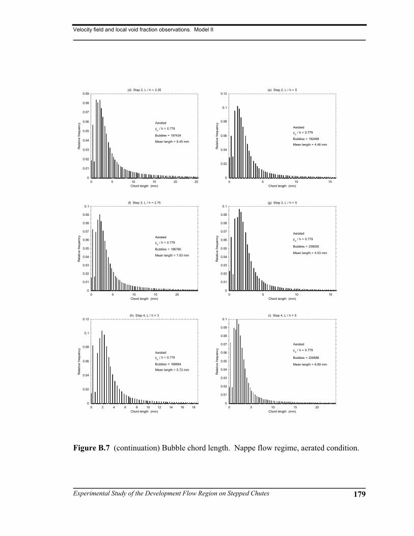
Velocity field and local void fraction observations. Model II
Experimental Study of the Development Flow Region on Stepped Chutes 179
0 5 10 15 20 250
0.01
0.02
0.03
0.04
0.05
0.06
0.07
0.08
0.09(d) Step 2, L / h = 2.25
Chord length (mm)
Rel
ativ
e fre
quen
cy Aerated
yc / h = 0.779
Bubbles = 197434
Mean length = 8.45 mm
0 5 10 150
0.02
0.04
0.06
0.08
0.1
0.12(e) Step 2, L / h = 5
Chord length (mm)
Rel
ativ
e fre
quen
cy
Aeratedyc / h = 0.779
Bubbles = 182489
Mean length = 4.46 mm
0 5 10 15 200
0.01
0.02
0.03
0.04
0.05
0.06
0.07
0.08
0.09
0.1(f) Step 3, L / h = 2.75
Chord length (mm)
Rel
ativ
e fre
quen
cy Aerated
yc / h = 0.779
Bubbles = 196760
Mean length = 7.83 mm
0 5 10 150
0.01
0.02
0.03
0.04
0.05
0.06
0.07
0.08
0.09
0.1(g) Step 3, L / h = 5
Chord length (mm)
Rel
ativ
e fre
quen
cy
Aerated
yc / h = 0.779
Bubbles = 259055
Mean length = 4.53 mm
0 2 4 6 8 10 12 14 16 180
0.02
0.04
0.06
0.08
0.1
0.12(h) Step 4, L / h = 3
Chord length (mm)
Rel
ativ
e fre
quen
cy
Aeratedyc / h = 0.779
Bubbles = 168884
Mean length = 5.72 mm
0 5 10 15 200
0.01
0.02
0.03
0.04
0.05
0.06
0.07
0.08
0.09
0.1(i) Step 4, L / h = 5
Chord length (mm)
Rel
ativ
e fre
quen
cy
Aerated
yc / h = 0.779
Bubbles = 200888
Mean length = 6.89 mm
Figure B.7 (continuation) Bubble chord length. Nappe flow regime, aerated condition.
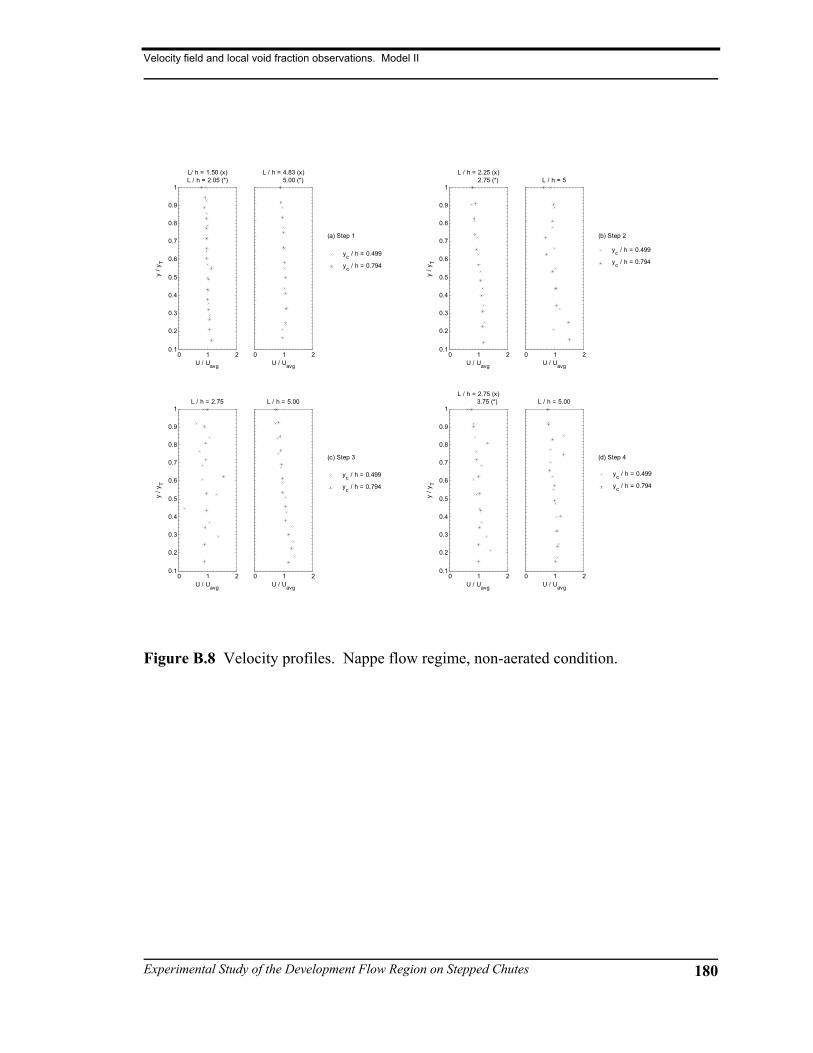
Velocity field and local void fraction observations. Model II
Experimental Study of the Development Flow Region on Stepped Chutes 180
0 1 20.1
0.2
0.3
0.4
0.5
0.6
0.7
0.8
0.9
1
L/ h = 1.50 (x)L / h = 2.05 (*)
U / Uavg
y / y
T
0 1 2
L / h = 4.83 (x) 5.00 (*)
U / Uavg
(a) Step 1
yc / h = 0.499
yc / h = 0.794
0 1 20.1
0.2
0.3
0.4
0.5
0.6
0.7
0.8
0.9
1
L / h = 2.25 (x) 2.75 (*)
U / Uavg
y / y
T
0 1 2
L / h = 5
U / Uavg
(b) Step 2
yc / h = 0.499
yc / h = 0.794
0 1 20.1
0.2
0.3
0.4
0.5
0.6
0.7
0.8
0.9
1
L / h = 2.75
U / Uavg
y / y
T
0 1 2
L / h = 5.00
U / Uavg
(c) Step 3
yc / h = 0.499
yc / h = 0.794
0 1 20.1
0.2
0.3
0.4
0.5
0.6
0.7
0.8
0.9
1
L / h = 2.75 (x) 3.75 (*)
U / Uavg
y / y
T
0 1 2
L / h = 5.00
U / Uavg
(d) Step 4
yc / h = 0.499
yc / h = 0.794
Figure B.8 Velocity profiles. Nappe flow regime, non-aerated condition.

Velocity field and local void fraction observations. Model II
Experimental Study of the Development Flow Region on Stepped Chutes 181
-1000 0 10000
0.1
0.2
0.3
0.4
0.5
0.6
0.7
0.8
0.9
1
L / h = 1.50 (x) 2.05 (*)
y / y
T
dU / dy (m / s / m)-1000 0 1000
L / h = 4.83 (x) 5.00 (*)
dU / dy (m / s / m)
(a) Step 1
yc / h = 0.499
yc / h = 0.794
-1000 0 10000
0.1
0.2
0.3
0.4
0.5
0.6
0.7
0.8
0.9
1
L / h = 2.25 (x) 2.75 (*)
y / y
T
dU / dy (m / s / m)-1000 0 1000
L / h = 5.00
dU / dy (m / s / m)
(b) Step 2
yc / h = 0.499
yc / h = 0.794
-1000 0 10000
0.1
0.2
0.3
0.4
0.5
0.6
0.7
0.8
0.9
1
L / h = 2.75
dU / dy (m / s / m)
y / y
T
-1000 0 1000
L / h = 5.00
dU / dy (m / s / m)
(c) Step 3
yc / h = 0.499
yc / h = 0.794
-1000 0 10000
0.1
0.2
0.3
0.4
0.5
0.6
0.7
0.8
0.9
1
L / h = 2.75 (x) 3.25 (*)
dU / dy (m / s / m)
y / y
T
-1000 0 1000
L / h = 5.00
dU / dy (m / s / m)
(d) Step 4
yc / h = 0.499
yc / h = 0.794
Figure B.9 Velocity gradient profiles. Nappe flow regime, non-aerated condition.

Velocity field and local void fraction observations. Model II
Experimental Study of the Development Flow Region on Stepped Chutes 182
0 0.50.1
0.2
0.3
0.4
0.5
0.6
0.7
0.8
0.9
1
L / h = 1.50 (x) 2.05 (*)
y / y
T
Tu0 0.5
L / h = 4.83 (x) 5.00 (*)
Tu
(a) Step 1
yc / h = 0.499
yc / h = 0.794
0 0.50.1
0.2
0.3
0.4
0.5
0.6
0.7
0.8
0.9
1
L / h = 2.25 (x) 2.75 (*)
y / y
T
Tu0 0.5
L / h = 5.00
Tu
(b) Step 2
yc / h = 0.499
yc / h = 0.794
0 0.50.1
0.2
0.3
0.4
0.5
0.6
0.7
0.8
0.9
1
L / h = 2.75
y / y
T
Tu0 0.5
L / h = 2.75
Tu
(c) Step 3
yc / h = 0.499
yc / h = 0.794
0 0.50.1
0.2
0.3
0.4
0.5
0.6
0.7
0.8
0.9
1
L / h = 2.75 (x) 3.75 (*)
y / y
T
Tu0 0.5
L / h = 5.00
Tu
(d) Step 4
yc / h = 0.499
yc / h = 0.794
Figure B.10 Turbulence intensity profiles. Nappe flow regime, non-aerated
condition.

Velocity field and local void fraction observations. Model II
Experimental Study of the Development Flow Region on Stepped Chutes 183
0 0.1 0.20.1
0.2
0.3
0.4
0.5
0.6
0.7
0.8
0.9
1
L / h = 1.50 (x) 2.05 (*)
y / y
T
u2 (m2 / s2)0 0.1 0.2
L / h = 4.83 (x) 5.00 (*)
u2 (m2 / s2)
(a) Step 1
yc / h = 0.499
yc / h = 0.794
0 0.1 0.20.1
0.2
0.3
0.4
0.5
0.6
0.7
0.8
0.9
1
L / h = 2.25 (x) 2.75 (*)
y / y
T
u2 (m2 / s2)0 0.1 0.2
L / h = 5.00 (x) 5.00 (*)
u2 (m2 / s2)
(b) Step 2
yc / h = 0.499
yc / h = 0.794
0 0.1 0.20.1
0.2
0.3
0.4
0.5
0.6
0.7
0.8
0.9
1
L / h = 2.75
y / y
T
u2 (m2 / s2)0 0.1 0.2
L / h = 2.75
u2 (m2 / s2)
(c) Step 3
yc / h = 0.499
yc / h = 0.794
0 0.1 0.20.1
0.2
0.3
0.4
0.5
0.6
0.7
0.8
0.9
1
L / h = 2.75 (x) 3.25 (*)
y / y
T
u2 (m2 / s2)0 0.1 0.2
L / h = 5.00
u2 (m2 / s2)
(d) Step 4
yc / h = 0.499
yc / h = 0.794
Figure B.11 Normal stress profiles. Nappe flow regime, non-aerated condition.
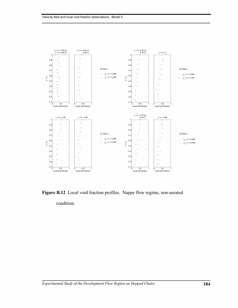
Velocity field and local void fraction observations. Model II
Experimental Study of the Development Flow Region on Stepped Chutes 184
0 0.5 10.1
0.2
0.3
0.4
0.5
0.6
0.7
0.8
0.9
1
L/ h = 1.50 (x)L / h = 2.05 (*)
Local void fraction
y / y
T
0 0.5 1
L / h = 4.83 (x) 5.00 (*)
Local void fraction
(a) Step 1
yc / h = 0.499
yc / h = 0.794
0 0.5 10.1
0.2
0.3
0.4
0.5
0.6
0.7
0.8
0.9
1
L / h = 2.25 (x) 2.75 (*)
Local void fraction
y / y
T
0 0.5 1
L / h = 5
Local void fraction
(b) Step 2
yc / h = 0.499
yc / h = 0.794
0 0.5 10.1
0.2
0.3
0.4
0.5
0.6
0.7
0.8
0.9
1
L / h = 2.75
Local void fraction
y / y
T
0 0.5 1
L / h = 5.00
Local void fraction
(c) Step 3
yc / h = 0.499
yc / h = 0.794
0 0.5 10.1
0.2
0.3
0.4
0.5
0.6
0.7
0.8
0.9
1
L / h = 2.75 (x) 3.75 (*)
Local voif fraction
y / y
T
0 0.5 1
L / h = 5.00
Local void fraction
(d) Step 4
yc / h = 0.499
yc / h = 0.794
Figure B.12 Local void fraction profiles. Nappe flow regime, non-aerated
condition.
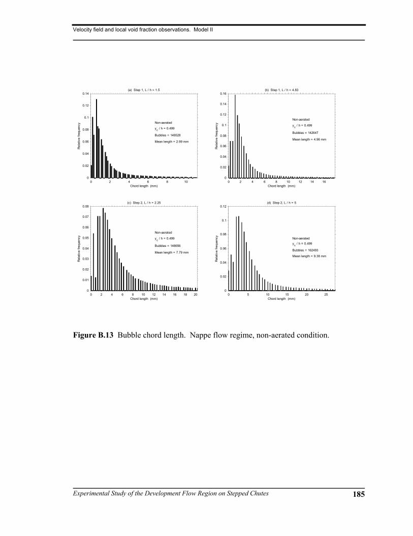
Velocity field and local void fraction observations. Model II
Experimental Study of the Development Flow Region on Stepped Chutes 185
0 2 4 6 8 100
0.02
0.04
0.06
0.08
0.1
0.12
0.14(a) Step 1, L / h = 1.5
Chord length (mm)
Rel
ativ
e fre
quen
cy
Non-aerated
yc / h = 0.499
Bubbles = 149528
Mean length = 2.99 mm
0 2 4 6 8 10 12 14 160
0.02
0.04
0.06
0.08
0.1
0.12
0.14
0.16(b) Step 1, L / h = 4.83
Chord length (mm)
Rel
ativ
e fre
quen
cy
Non-aerated
yc / h = 0.499
Bubbles = 142647
Mean length = 4.96 mm
0 2 4 6 8 10 12 14 16 18 200
0.01
0.02
0.03
0.04
0.05
0.06
0.07
0.08(c) Step 2, L / h = 2.25
Chord length (mm)
Rel
ativ
e fre
quen
cy
Non-aerated
yc / h = 0.499
Bubbles = 148656
Mean length = 7.79 mm
0 5 10 15 20 250
0.02
0.04
0.06
0.08
0.1
0.12(d) Step 2, L / h = 5
Chord length (mm)
Rel
ativ
e fre
quen
cy Non-aeratedyc / h = 0.499
Bubbles = 162493
Mean length = 9.38 mm
Figure B.13 Bubble chord length. Nappe flow regime, non-aerated condition.

Velocity field and local void fraction observations. Model II
Experimental Study of the Development Flow Region on Stepped Chutes 186
0 5 10 15 20 250
0.01
0.02
0.03
0.04
0.05
0.06
0.07
0.08(e) Step 3, L / h = 2.75
Chord length (mm)
Rel
ativ
e fre
quen
cy Non-aeratedyc / h = 0.499
Bubbles = 142830
Mean length = 8.98 mm
0 2 4 6 8 10 12 14 16 180
0.01
0.02
0.03
0.04
0.05
0.06
0.07
0.08
0.09(f) Step 3, L / h = 5
Chord length (mm)
Rel
ativ
e fre
quen
cy
Non-aerated
yc / h = 0.499
Bubbles = 177446
Mean length = 5.38 mm
0 2 4 6 8 10 12 14 16 180
0.01
0.02
0.03
0.04
0.05
0.06
0.07
0.08(g) Step 4, L / h = 2.75
Chord length (mm)
Rel
ativ
e fre
quen
cy
Non-aerated
yc / h = 0.499
Bubbles = 199727
Mean length = 6.59 mm
0 5 10 15 200
0.01
0.02
0.03
0.04
0.05
0.06
0.07
0.08
0.09(h) Step 4, L / h = 5
Chord length (mm)
Rel
ativ
e fre
quen
cy
Non-aerated
yc / h = 0.499
Bubbles = 214962
Mean length = 7.33 mm
Figure B.13 (continuation) Bubble chord length. Nappe flow regime, non-
aerated condition.

Velocity field and local void fraction observations. Model II
Experimental Study of the Development Flow Region on Stepped Chutes 187
0 2 4 6 8 10 12 14 16 180
0.02
0.04
0.06
0.08
0.1
0.12
0.14
0.16(a) Step 1, L / h = 2.05
Chord length (mm)
Rel
ativ
e fre
quen
cy
Non-aerated
yc / h = 0.794
Bubbles = 160955
Mean length = 4.98 mm
0 2 4 6 8 10 12 14 16 18 200
0.02
0.04
0.06
0.08
0.1
0.12
0.14
0.16(b) Step 1, L / h = 5
Chord length (mm)
Rel
ativ
e fre
quen
cy
Non-aerated
yc / h = 0.794
Bubbles = 189539
Mean length = 5.97 mm
0 5 10 150
0.01
0.02
0.03
0.04
0.05
0.06
0.07
0.08
0.09(c) Step 2, L / h = 2.75
Chord length (mm)
Rel
ativ
e fre
quen
cy Non-aerated
yc / h = 0.794
Bubbles = 182802
Mean length = 5.59 mm
0 2 4 6 8 10 12 14 160
0.02
0.04
0.06
0.08
0.1
0.12(d) Step 2, L / h = 5
Chord length (mm)
Rel
ativ
e fre
quen
cy
Non-aeratedyc / h = 0.794
Bubbles = 163702
Mean length = 5.29 mm
Figure B.14 Bubble chord length. Nappe flow regime, non-aerated condition.

Velocity field and local void fraction observations. Model II
Experimental Study of the Development Flow Region on Stepped Chutes 188
0 5 10 15 20 25 300
0.01
0.02
0.03
0.04
0.05
0.06
0.07
0.08
0.09(e) Step 3, L / h = 2.75
Chord length (mm)
Rel
ativ
e fre
quen
cy
Non-aerated
yc / h = 0.794
Bubbles = 176398
Mean length = 11.8 mm
0 2 4 6 8 10 12 14 16 180
0.02
0.04
0.06
0.08
0.1
0.12(f) Step 3, L / h = 5
Chord length (mm)
Rel
ativ
e fre
quen
cy
Non-aeratedyc / h = 0.794
Bubbles = 250731
Mean length = 6.6 mm
0 5 10 15 200
0.02
0.04
0.06
0.08
0.1
0.12(g) Step 4, L / h = 3.75
Chord length (mm)
Rel
ativ
e fre
quen
cy
Non-aeratedyc / h = 0.794
Bubbles = 172022
Mean length = 7.67 mm
0 5 10 15 20 250
0.01
0.02
0.03
0.04
0.05
0.06
0.07
0.08
0.09
0.1(h) Step 4, L / h = 5
Chord length (mm)
Rel
ativ
e fre
quen
cy
Non-aerated
yc / h = 0.794
Bubbles = 179020
Mean length = 7.34 mm
Figure B.14 (continuation) Bubble chord length. Nappe flow regime, non-
aerated condition.
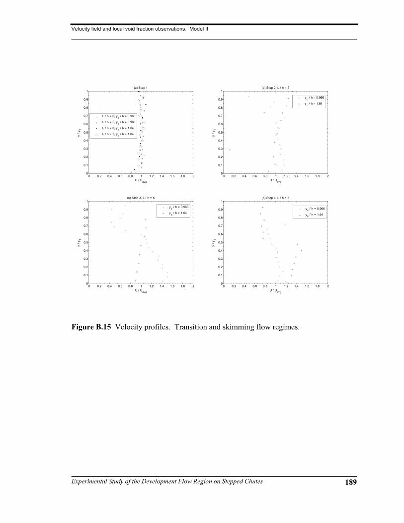
Velocity field and local void fraction observations. Model II
Experimental Study of the Development Flow Region on Stepped Chutes 189
0 0.2 0.4 0.6 0.8 1 1.2 1.4 1.6 1.8 20
0.1
0.2
0.3
0.4
0.5
0.6
0.7
0.8
0.9
1(a) Step 1
U / Uavg
y / y
T
L / h = 0, yc / h = 0.966
L / h = 5, yc / h = 0.966
L / h = 0, yc / h = 1.64
L / h = 5, yc / h = 1.64
0 0.2 0.4 0.6 0.8 1 1.2 1.4 1.6 1.8 20
0.1
0.2
0.3
0.4
0.5
0.6
0.7
0.8
0.9
1(b) Step 2, L / h = 5
U / Uavg
y / y
T
yc / h = 0.966
yc / h = 1.64
0 0.2 0.4 0.6 0.8 1 1.2 1.4 1.6 1.8 20
0.1
0.2
0.3
0.4
0.5
0.6
0.7
0.8
0.9
1(c) Step 3, L / h = 5
U / Uavg
y / y
T
yc / h = 0.966
yc / h = 1.64
0 0.2 0.4 0.6 0.8 1 1.2 1.4 1.6 1.8 20
0.1
0.2
0.3
0.4
0.5
0.6
0.7
0.8
0.9
1(d) Step 4, L / h = 5
U / Uavg
y / y
T
yc / h = 0.966
yc / h = 1.64
Figure B.15 Velocity profiles. Transition and skimming flow regimes.

Velocity field and local void fraction observations. Model II
Experimental Study of the Development Flow Region on Stepped Chutes 190
-400 -300 -200 -100 0 100 200 300 4000
0.1
0.2
0.3
0.4
0.5
0.6
0.7
0.8
0.9
1(a) Step 1
dU / dy (m /s /m)
y / y
T
L / h = 0, yc / h = 0.966
L / h = 5, yc / h = 0.966
L / h = 0, yc / h = 1.64
L / h = 5, yc / h = 1.64
-400 -300 -200 -100 0 100 200 300 4000
0.1
0.2
0.3
0.4
0.5
0.6
0.7
0.8
0.9
1(b) Step 2, L / h = 5
dU / dy (m / s / m)
y / y
T
yc / h = 0.966
yc / h = 1.64
-400 -300 -200 -100 0 100 200 300 4000
0.1
0.2
0.3
0.4
0.5
0.6
0.7
0.8
0.9
1(c) Step 3, L / h = 5
dU / dy (m / s /m)
y / y
T
yc / h = 0.966
yc / h = 1.64
-400 -300 -200 -100 0 100 200 300 4000
0.1
0.2
0.3
0.4
0.5
0.6
0.7
0.8
0.9
1(d) Step 4, L / h = 5
dU / dy (m /s / m)
y / y
T
yc / h = 0.966
yc / h = 1.64
Figure B.16 Velocity gradient profiles. Transition and skimming flow regimes.

Velocity field and local void fraction observations. Model II
Experimental Study of the Development Flow Region on Stepped Chutes 191
0 0.05 0.1 0.150
0.1
0.2
0.3
0.4
0.5
0.6
0.7
0.8
0.9
1(a) Step 1
Tu
y / y
T
L / h = 0, yc / h = 0.966
L / h = 5, yc / h = 0.966
L / h = 0, yc / h = 1.64
L / h = 5, yc / h = 1.64
0 0.05 0.1 0.150
0.1
0.2
0.3
0.4
0.5
0.6
0.7
0.8
0.9
1(b) Step 2, L / h = 5
Tu
y / y
T
yc / h = 0.966
yc / h = 1.64
0 0.05 0.1 0.150
0.1
0.2
0.3
0.4
0.5
0.6
0.7
0.8
0.9
1(c) Step 3, L / h = 5
Tu
y / y
T
yc / h = 0.966
yc / h = 1.64
0 0.05 0.1 0.150
0.1
0.2
0.3
0.4
0.5
0.6
0.7
0.8
0.9
1(d) Step 4, L / h = 5
Tu
y / y
T
yc / h = 0.966
yc / h = 1.64
Figure B.17 Turbulence intensity profiles. Transition and skimming flow
regimes.

Velocity field and local void fraction observations. Model II
Experimental Study of the Development Flow Region on Stepped Chutes 192
0 0.02 0.04 0.06 0.08 0.1 0.12 0.14 0.16 0.18 0.20
0.1
0.2
0.3
0.4
0.5
0.6
0.7
0.8
0.9
1(a) Step 1
u2 (m2 / s2)
y / y
T
L / h = 0, yc / h = 0.966
L / h = 5, yc / h = 0.966
L / h = 0, yc / h = 1.64
L / h = 5, yc / h = 1.64
0 0.02 0.04 0.06 0.08 0.1 0.12 0.14 0.16 0.18 0.20
0.1
0.2
0.3
0.4
0.5
0.6
0.7
0.8
0.9
1(b) Step 2, L / h = 5
u2 (m2 / s2)
y / y
T
yc / h = 0.966
yc / h = 1.64
0 0.02 0.04 0.06 0.08 0.1 0.12 0.14 0.16 0.18 0.20
0.1
0.2
0.3
0.4
0.5
0.6
0.7
0.8
0.9
1(c) Step 3, L / h = 5
u2 (m2 / s2)
y / y
T
yc / h = 0.966
yc / h = 1.64
0 0.02 0.04 0.06 0.08 0.1 0.12 0.14 0.16 0.18 0.20
0.1
0.2
0.3
0.4
0.5
0.6
0.7
0.8
0.9
1(d) Step 4, L / h = 5
u2 (m2 / s2)
y / y
T
yc / h = 0.966
yc / h = 1.64
Figure B.18 Normal stress profiles. Transition and skimming flow regimes.

Velocity field and local void fraction observations. Model II
Experimental Study of the Development Flow Region on Stepped Chutes 193
0 0.1 0.2 0.3 0.4 0.5 0.6 0.7 0.8 0.9 10
0.1
0.2
0.3
0.4
0.5
0.6
0.7
0.8
0.9
1(a) Step 1
Local void fraction
y / y
T
L / h = 0, yc / h = 0.966
L / h = 5, yc / h = 0.966
L / h = 0, yc / h = 1.64
L / h = 5, yc / h = 1.64
0 0.1 0.2 0.3 0.4 0.5 0.6 0.7 0.8 0.9 10
0.1
0.2
0.3
0.4
0.5
0.6
0.7
0.8
0.9
1(b) Step 2, L / h = 5
Local void fraction
y / y
T
yc / h = 0.966
yc / h = 1.64
0 0.1 0.2 0.3 0.4 0.5 0.6 0.7 0.8 0.9 10
0.1
0.2
0.3
0.4
0.5
0.6
0.7
0.8
0.9
1(c) Step 3, L / h = 5
Local void fraction
y / y
T
yc / h = 0.966
yc / h = 1.64
0 0.1 0.2 0.3 0.4 0.5 0.6 0.7 0.8 0.9 10
0.1
0.2
0.3
0.4
0.5
0.6
0.7
0.8
0.9
1(d) Step 4, L / h = 5
Local void fraction
y / y
T
yc / h = 0.966
yc / h = 1.64
Figure B.19 Local void fraction profiles. Transition and skimming flow regimes.

Velocity field and local void fraction observations. Model II
Experimental Study of the Development Flow Region on Stepped Chutes 194
0 1 2 3 4 5 6 70
0.05
0.1
0.15
0.2
0.25
0.3
0.35(a) Step 1, L / h = 0
Chord length (mm)
Rel
ativ
e fre
quen
cy
Non-aeratedyc / h = 0.966
Bubbles = 20236Mean length = 1.4 mm
0 5 10 15 20 250
0.02
0.04
0.06
0.08
0.1
0.12
0.14
0.16
0.18(b) Step 1, L / h = 5
Chord length (mm)
Rel
ativ
e fre
quen
cy Non-aerated
yc / h = 0.966
Bubbles = 26452
Mean length = 7.34 mm
0 2 4 6 8 10 12 14 16 18 200
0.02
0.04
0.06
0.08
0.1
0.12
0.14(c) Step 2, L / h = 5
Chord length (mm)
Rel
ativ
e fre
quen
cy Non-aeratedyc / h = 0.966
Bubbles = 237689
Mean length = 6.66 mm
0 5 10 15 20 250
0.02
0.04
0.06
0.08
0.1
0.12(d) Step 3, L / h = 5
Chord length (mm)
Rel
ativ
e fre
quen
cy
Non-aeratedyc / h = 0.966
Bubbles = 296438
Mean length = 8.41 mm
Figure B.20 Bubble chord length. Transition flow regime.

Velocity field and local void fraction observations. Model II
Experimental Study of the Development Flow Region on Stepped Chutes 195
0 2 4 6 8 10 12 140
0.05
0.1
0.15
0.2
0.25
0.3
0.35(a) Step 1, L / h = 0
Chord length (mm)
Rel
ativ
e fre
quen
cy
Non-aeratedyc / h = 1.64
Bubbles = 42804Mean length = 3.83 mm
0 2 4 6 8 10 12 14 16 18 200
0.05
0.1
0.15
0.2
0.25(b) Step 1, L / h = 5
Chord length (mm)
Rel
ativ
e fre
quen
cy Non-aerated
yc / h = 1.64
Bubbles = 25194
Mean length = 5.79 mm
0 5 10 15 20 250
0.02
0.04
0.06
0.08
0.1
0.12
0.14
0.16
0.18
0.2(c) Step 2, L / h = 5
Chord length (mm)
Rel
ativ
e fre
quen
cy
Non-aerated
yc / h = 1.64
Bubbles = 39876
Mean length = 8.54 mm
0 5 10 15 20 25 30 350
0.02
0.04
0.06
0.08
0.1
0.12
0.14
0.16(d) Step 3, L / h = 5
Chord length (mm)
Rel
ativ
e fre
quen
cy Non-aerated
yc / h = 1.64
Bubbles = 20150
Mean length = 12.2 mm
0 5 10 15 20 25 300
0.02
0.04
0.06
0.08
0.1
0.12(e) Step 4, L / h = 5
Chord length (mm)
Rel
ativ
e fre
quen
cy Non-aerated
yc / h = 1.64
Bubbles = 214526
Mean length = 11.3 mm
Figure B.21 Bubble chord length. Skimming flow regime.
Velocity field and local void fraction observations. Model III
Experimental Study of the Development Flow Region on Stepped Chutes 196
Appendix C Velocity field and local void fraction
observations. Model III

Velocity field and local void fraction observations. Model III
Experimental Study of the Development Flow Region on Stepped Chutes 197
0 0.5 1 1.50
0.1
0.2
0.3
0.4
0.5
0.6
0.7
0.8
0.9
1
L / h = 0
y / y
T
0 0.5 1 1.5
L / h = 2.00 (x) 2.50 (*)
U / Uavg
0 0.5 1 1.5
L / h = 10
(a) Step 1
yc / h = 0.492
yc / h = 0.798
0 0.5 1 1.50
0.1
0.2
0.3
0.4
0.5
0.6
0.7
0.8
0.9
1
L / h = 0
y / y
T
0 0.5 1 1.5
L / h = 2.50
U / Uavg
0 0.5 1 1.5
L / h = 10
(b) Step 2
yc / h = 0.492
yc / h = 0.798
0 0.5 1 1.50
0.1
0.2
0.3
0.4
0.5
0.6
0.7
0.8
0.9
1
L / h = 0
y / y
T
0 0.5 1 1.5
L / h = 2.50
U / Uavg
0 0.5 1 1.5
L / h = 10
(c) Step 3
yc / h = 0.492
yc / h = 0.798
0 0.5 1 1.50
0.1
0.2
0.3
0.4
0.5
0.6
0.7
0.8
0.9
1
L / h = 0
y / y
T
0 0.5 1 1.5
L / h = 2.50 (x) 3.00 (*)
U / Uavg
0 0.5 1 1.5
L / h = 10
(d) Step 4
yc / h = 0.492
yc / h = 0.798
Figure C.1 Velocity profiles. Nappe flow regime, aerated condition.

Velocity field and local void fraction observations. Model III
Experimental Study of the Development Flow Region on Stepped Chutes 198
-1000 0 10000
0.1
0.2
0.3
0.4
0.5
0.6
0.7
0.8
0.9
1
L / h = 0
y / y
T
-1000 0 1000
L / h = 2.00 (x) 2.50 (*)
dU / dy (m / s / m)-1000 0 1000
L / h = 10
(a) Step 1
yc / h = 0.492
yc / h = 0.798
-1000 0 10000
0.1
0.2
0.3
0.4
0.5
0.6
0.7
0.8
0.9
1
L / h = 0
y / y
T
-1000 0 1000
L / h = 2.50
dU / dy (m / s / m)-1000 0 1000
L / h = 10
(b) Step 2
yc / h = 0.492
yc / h = 0.798
-1000 0 10000
0.1
0.2
0.3
0.4
0.5
0.6
0.7
0.8
0.9
1
L / h = 0
y / y
T
-1000 0 1000
L / h = 2.50 (x) 3.00 (*)
dU / dy (m / s / m)-1000 0 1000
L / h = 10
(c) Step 3
yc / h = 0.492
yc / h = 0.798
-1000 0 10000
0.1
0.2
0.3
0.4
0.5
0.6
0.7
0.8
0.9
1
L / h = 0
y / y
T
-1000 0 1000
L / h = 2.50 (x) 3.00 (*)
dU / dy (m / s / m)-1000 0 1000
L / h = 10
(d) Step 4
yc / h = 0.492
yc / h = 0.798
Figure C.2 Velocity gradient profiles. Nappe flow regime, aerated condition.

Velocity field and local void fraction observations. Model III
Experimental Study of the Development Flow Region on Stepped Chutes 199
0 0.50
0.1
0.2
0.3
0.4
0.5
0.6
0.7
0.8
0.9
1
L / h = 0
y / y
T
0 0.5
L / h = 2.00 (x) 2.50 (*)
Tu0 0.5
L / h = 10
(a) Step 1
yc / h = 0.492
yc / h = 0.798
0 0.50
0.1
0.2
0.3
0.4
0.5
0.6
0.7
0.8
0.9
1
L / h = 0
y / y
T
0 0.5
L / h = 2.50
Tu0 0.5
L / h = 10
(b) Step 2
yc / h = 0.492
yc / h = 0.798
0 0.50
0.1
0.2
0.3
0.4
0.5
0.6
0.7
0.8
0.9
1
L / h = 0
y / y
T
0 0.5
L / h = 2.50 (x) 3.00 (*)
Tu0 0.5
L / h = 10
(c) Step 3
yc / h = 0.492
yc / h = 0.798
0 0.50
0.1
0.2
0.3
0.4
0.5
0.6
0.7
0.8
0.9
1
L / h = 0
y / y
T
0 0.5
L / h = 2.50 (x) 3.00 (*)
Tu0 0.5
L / h = 10
(d) Step 4
yc / h = 0.492
yc / h = 0.798
Figure C.3 Turbulence intensity profiles. Nappe flow regime, aerated condition.

Velocity field and local void fraction observations. Model III
Experimental Study of the Development Flow Region on Stepped Chutes 200
0 0.50
0.1
0.2
0.3
0.4
0.5
0.6
0.7
0.8
0.9
1
L / h = 0
y / y
T
0 0.5
L / h = 2.00 (x) 2.50 (*)
u2 (m2 / s2)0 0.5
L / h = 10
(a) Step 1
yc / h = 0.492
yc / h = 0.779
0 0.50
0.1
0.2
0.3
0.4
0.5
0.6
0.7
0.8
0.9
1
L / h = 0
y / y
T
0 0.5
L / h = 2.50
u2 (m2 / s2)0 0.5
L / h = 10
(b) Step 2
yc / h = 0.492
yc / h = 0.779
0 0.50
0.1
0.2
0.3
0.4
0.5
0.6
0.7
0.8
0.9
1
L / h = 0
y / y
T
0 0.5
L / h = 2.50 (x) 3.00 (*)
u2 (m2 / s2)0 0.5
L / h = 10
(c) Step 3
yc / h = 0.492
yc / h = 0.779
0 0.50
0.1
0.2
0.3
0.4
0.5
0.6
0.7
0.8
0.9
1
L / h = 0
y / y
T
0 0.5
L / h = 2.50 (x) 3.00 (*)
u2 (m2 / s2)0 0.5
L / h = 10
(d) Step 4
yc / h = 0.492
yc / h = 0.779
Figure C.4 Normal stresss profiles. Nappe flow regime, aerated condition.

Velocity field and local void fraction observations. Model III
Experimental Study of the Development Flow Region on Stepped Chutes 201
0 0.5 10
0.1
0.2
0.3
0.4
0.5
0.6
0.7
0.8
0.9
1
L / h = 0
y / y
T
0 0.5 1
L / h = 2.00 (x) 2.50 (*)
Local void fraction0 0.5 1
L / h = 10
(a) Step 1
yc / h = 0.492
yc / h = 0.798
0 0.5 10
0.1
0.2
0.3
0.4
0.5
0.6
0.7
0.8
0.9
1
L / h = 0
y / y
T
0 0.5 1
L / h = 2.50
Local void fraction0 0.5 1
L / h = 10
(b) Step 2
yc / h = 0.492
yc / h = 0.798
0 0.5 10
0.1
0.2
0.3
0.4
0.5
0.6
0.7
0.8
0.9
1
L / h = 0
y / y
T
0 0.5 1
L / h = 2.50
Local void fraction0 0.5 1
L / h = 10
(c) Step 3
yc / h = 0.492
yc / h = 0.798
0 0.5 10
0.1
0.2
0.3
0.4
0.5
0.6
0.7
0.8
0.9
1
L / h = 0
y / y
T
0 0.5 1
L / h = 2.50 (x) 3.00 (*)
Local void fraction0 0.5 1
L / h = 10
(d) Step 4
yc / h = 0.492
yc / h = 0.798
Figure C.5 Local void fraction profiles. Nappe flow regime, aerated condition.
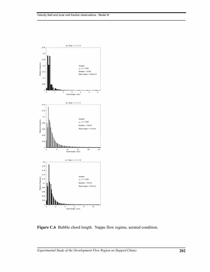
Velocity field and local void fraction observations. Model III
Experimental Study of the Development Flow Region on Stepped Chutes 202
0 1 2 3 4 5 60
0.05
0.1
0.15
0.2
0.25
0.3
0.35(a) Step 1, L / h = 0
Chord length (mm)
Rel
ativ
e fre
quen
cy
Aeratedyc / h = 0.492
Bubbles = 21355
Mean length = 0.944 mm
0 5 10 15 20 250
0.02
0.04
0.06
0.08
0.1
0.12
0.14(b) Step 1, L / h = 2
Chord length (mm)
Rel
ativ
e fre
quen
cy
Aerated
yc / h = 0.492
Bubbles = 100102
Mean length = 7.35 mm
0 2 4 6 8 100
0.02
0.04
0.06
0.08
0.1
0.12
0.14
0.16
0.18
0.2(c) Step 1, L / h = 10
Chord length (mm)
Rel
ativ
e fre
quen
cy
Aerated
yc / h = 0.492
Bubbles = 164116
Mean length = 2.63 mm
Figure C.6 Bubble chord length. Nappe flow regime, aerated condition.

Velocity field and local void fraction observations. Model III
Experimental Study of the Development Flow Region on Stepped Chutes 203
0 5 10 15 20 25 300
0.01
0.02
0.03
0.04
0.05
0.06
0.07
0.08
0.09(d) Step 2, L / h = 2.5
Chord length (mm)
Rel
ativ
e fre
quen
cy
Aerated
yc / h = 0.492
Bubbles = 92137
Mean length = 10.4 mm
0 2 4 6 8 10 12 14 16 180
0.02
0.04
0.06
0.08
0.1
0.12
0.14
0.16
0.18(e) Step 2, L / h = 10
Chord length (mm)
Rel
ativ
e fre
quen
cy
Aerated
yc / h = 0.492
Bubbles = 160850
Mean length = 4.62 mm
0 5 10 15 20 250
0.01
0.02
0.03
0.04
0.05
0.06
0.07
0.08(f) Step 3, L / h = 2.5
Chord length (mm)
Rel
ativ
e fre
quen
cy
Aerated
yc / h = 0.492
Bubbles = 121498
Mean length = 9.72 mm
0 5 10 15 20 250
0.02
0.04
0.06
0.08
0.1
0.12
0.14
0.16(g) Step 3, L / h = 10
Chord length (mm)
Rel
ativ
e fre
quen
cy Aerated
yc / h = 0.492
Bubbles = 162310
Mean length = 7.27 mm
0 5 10 15 20 25 300
0.01
0.02
0.03
0.04
0.05
0.06
0.07
0.08(h) Step 4, L / h = 2.5
Chord length (mm)
Rel
ativ
e fre
quen
cy Aeratedyc / h = 0.492
Bubbles = 94927
Mean length = 12.3 mm
0 5 10 15 200
0.02
0.04
0.06
0.08
0.1
0.12
0.14
0.16(i) Step 4, L / h = 10
Chord length (mm)
Rel
ativ
e fre
quen
cy Aerated
yc / h = 0.492
Bubbles = 161248
Mean length = 5.93 mm
Figure C.6 (continuation) Bubble chord length. Nappe flow regime, aerated
condition.

Velocity field and local void fraction observations. Model III
Experimental Study of the Development Flow Region on Stepped Chutes 204
0 0.5 1 1.5 2 2.5 3 3.5 4 4.50
0.05
0.1
0.15
0.2
0.25
0.3
0.35(a) Step 1, L / h = 0
Chord length (mm)
Rel
ativ
e fre
quen
cy
Aeratedyc / h = 0.798
Bubbles = 33088
Mean length = 0.779 mm
0 2 4 6 8 10 12 14 16 180
0.02
0.04
0.06
0.08
0.1
0.12
0.14(b) Step 1, L / h = 2.5
Chord length (mm)
Rel
ativ
e fre
quen
cy
Aerated
yc / h = 0.798
Bubbles = 110213
Mean length = 5.21 mm
0 2 4 6 8 100
0.05
0.1
0.15
0.2
0.25(c) Step 1, L / h = 10
Chord length (mm)
Rel
ativ
e fre
quen
cy
Aeratedyc / h = 0.798
Bubbles = 189933
Mean length = 2.53 mm
Figure C.7 Bubble chord length. Nappe flow regime, aerated condition.

Velocity field and local void fraction observations. Model III
Experimental Study of the Development Flow Region on Stepped Chutes 205
0 2 4 6 8 10 12 14 160
0.01
0.02
0.03
0.04
0.05
0.06
0.07
0.08
0.09(d) Step 2, L / h = 2.5
Chord length (mm)
Rel
ativ
e fre
quen
cy
Aerated
yc / h = 0.798
Bubbles = 180469
Mean length = 5.52 mm
0 2 4 6 8 10 12 14 16 180
0.02
0.04
0.06
0.08
0.1
0.12
0.14
0.16
0.18(e) Step 2, L / h = 10
Chord length (mm)
Rel
ativ
e fre
quen
cy
Aerated
yc / h = 0.798
Bubbles = 243750
Mean length = 4.57 mm
0 5 10 15 20 250
0.02
0.04
0.06
0.08
0.1
0.12(f) Step 3, L / h = 3
Chord length (mm)
Rel
ativ
e fre
quen
cy
Aeratedyc / h = 0.798
Bubbles = 146060
Mean length = 9.9 mm
0 5 10 15 20 250
0.02
0.04
0.06
0.08
0.1
0.12
0.14
0.16(g) Step 3, L / h = 10
Chord length (mm)
Rel
ativ
e fre
quen
cy Aerated
yc / h = 0.798
Bubbles = 176647
Mean length = 7.55 mm
0 5 10 15 200
0.01
0.02
0.03
0.04
0.05
0.06
0.07
0.08
0.09(h) Step 4, L / h = 3
Chord length (mm)
Rel
ativ
e fre
quen
cy
Aerated
yc / h = 0.798
Bubbles = 167680
Mean length = 7.82 mm
0 2 4 6 8 10 12 14 16 18 200
0.02
0.04
0.06
0.08
0.1
0.12
0.14(i) Step 4, L / h = 10
Chord length (mm)
Rel
ativ
e fre
quen
cy Aerated
yc / h = 0.798
Bubbles = 241320
Mean length = 5.9 mm
Figure C.7 (continuation) Bubble chord length. Nappe flow regime, aerated
condition.
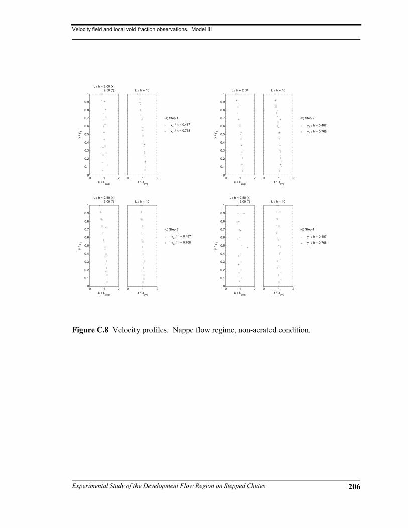
Velocity field and local void fraction observations. Model III
Experimental Study of the Development Flow Region on Stepped Chutes 206
0 1 20
0.1
0.2
0.3
0.4
0.5
0.6
0.7
0.8
0.9
1
L / h = 2.00 (x) 2.50 (*)
U / Uavg
y / y
T
0 1 2
L / h = 10
U / Uavg
(a) Step 1
yc / h = 0.487
yc / h = 0.768
0 1 20
0.1
0.2
0.3
0.4
0.5
0.6
0.7
0.8
0.9
1
L / h = 2.50
U / Uavg
y / y
T
0 1 2
L / h = 10
U / Uavg
(b) Step 2
yc / h = 0.487
yc / h = 0.768
0 1 20
0.1
0.2
0.3
0.4
0.5
0.6
0.7
0.8
0.9
1
L / h = 2.50 (x) 3.00 (*)
U / Uavg
y / y
T
0 1 2
L / h = 10
U / Uavg
(c) Step 3
yc / h = 0.487
yc / h = 0.768
0 1 20
0.1
0.2
0.3
0.4
0.5
0.6
0.7
0.8
0.9
1
L / h = 2.50 (x) 3.00 (*)
U / Uavg
y / y
T
0 1 2
L / h = 10
U / Uavg
(d) Step 4
yc / h = 0.487
yc / h = 0.768
Figure C.8 Velocity profiles. Nappe flow regime, non-aerated condition.

Velocity field and local void fraction observations. Model III
Experimental Study of the Development Flow Region on Stepped Chutes 207
-1000 0 10000
0.1
0.2
0.3
0.4
0.5
0.6
0.7
0.8
0.9
1
L / h = 2.00 (x) 2.50 (*)
y / y
T
dU / dy (m / s / m)-1000 0 1000
L / h = 10
dU / dy (m / s / m)
(a) Step 1
yc / h = 0.487
yc / h = 0.768
-1000 0 10000
0.1
0.2
0.3
0.4
0.5
0.6
0.7
0.8
0.9
1
L / h = 2.50
y / y
T
dU / dy (m / s / m)-1000 0 1000
L / h = 10
dU / dy (m / s / m)
(b) Step 2
yc / h = 0.487
yc / h = 0.768
-1000 0 10000
0.1
0.2
0.3
0.4
0.5
0.6
0.7
0.8
0.9
1
L / h = 2.50 (x) 3.00 (*)
dU / dy (m / s / m)
y / y
T
-1000 0 1000
L / h = 10
dU / dy (m / s / m)
(c) Step 3
yc / h = 0.487
yc / h = 0.768
-1000 0 10000
0.1
0.2
0.3
0.4
0.5
0.6
0.7
0.8
0.9
1
L / h = 2.50 (x) 3.00 (*)
dU / dy (m / s / m)
y / y
T
-1000 0 1000
L / h = 10
dU / dy (m / s / m)
(d) Step 4
yc / h = 0.487
yc / h = 0.768
Figure C.9 Velocity gradient profiles. Nappe flow regime, non-aerated
condition.

Velocity field and local void fraction observations. Model III
Experimental Study of the Development Flow Region on Stepped Chutes 208
0 0.50
0.1
0.2
0.3
0.4
0.5
0.6
0.7
0.8
0.9
1
L / h = 2.00 (x) 2.50 (*)
y / y
T
Tu0 0.5
L / h = 10
Tu
(a) Step 1
yc / h = 0.487
yc / h = 0.768
0 0.50
0.1
0.2
0.3
0.4
0.5
0.6
0.7
0.8
0.9
1
L / h = 2.50
y / y
T
Tu0 0.5
L / h = 10
Tu
(b) Step 2
yc / h = 0.487
yc / h = 0.768
0 0.50
0.1
0.2
0.3
0.4
0.5
0.6
0.7
0.8
0.9
1
L / h = 2.50 (x) 3.00 (*)
y / y
T
Tu0 0.5
L / h = 10
Tu
(c) Step 3
yc / h = 0.487
yc / h = 0.768
0 0.50
0.1
0.2
0.3
0.4
0.5
0.6
0.7
0.8
0.9
1
L / h = 2.50 (x) 3.00 (*)
y / y
T
Tu0 0.5
L / h = 10
Tu
(d) Step 4
yc / h = 0.487
yc / h = 0.768
Figure C.10 Turbulence intensity profiles. Nappe flow regime, non-aerated
condition.

Velocity field and local void fraction observations. Model III
Experimental Study of the Development Flow Region on Stepped Chutes 209
0 0.05 0.10
0.1
0.2
0.3
0.4
0.5
0.6
0.7
0.8
0.9
1
L / h = 2.00 (x) 2.50 (*)
y / y
T
u2 (m2 / s2)0 0.05 0.1
L / h = 10
u2 (m2 / s2)
(a) Step 1
yc / h = 0.487
yc / h = 0.768
0 0.05 0.10
0.1
0.2
0.3
0.4
0.5
0.6
0.7
0.8
0.9
1
L / h = 2.50
y / y
T
u2 (m2 / s2)0 0.05 0.1
L / h = 10
u2 (m2 / s2)
(b) Step 2
yc / h = 0.487
yc / h = 0.768
0 0.05 0.10
0.1
0.2
0.3
0.4
0.5
0.6
0.7
0.8
0.9
1
L / h = 2.50 (x) 3.00 (*)
y / y
T
u2 (m2 / s2)0 0.05 0.1
L / h = 10
u2 (m2 / s2)
(c) Step 3
yc / h = 0.487
yc / h = 0.768
0 0.05 0.10
0.1
0.2
0.3
0.4
0.5
0.6
0.7
0.8
0.9
1
L / h = 2.50 (x) 3.00 (*)
y / y
T
u2 (m2 / s2)0 0.05 0.1
L / h = 10
u2 (m2 / s2)
(d) Step 4
yc / h = 0.487
yc / h = 0.768
Figure C.11 Normal stress profiles. Nappe flow regime, non-aerated condition.
Velocity field and local void fraction observations. Model III
Experimental Study of the Development Flow Region on Stepped Chutes 210
0 0.5 10
0.1
0.2
0.3
0.4
0.5
0.6
0.7
0.8
0.9
1
L/ h = 2.0 (x)L / h = 2.5 (*)
Local void fraction
y / y
T
0 0.5 1
L / h = 10
Local void fraction
(a) Step 1
yc / h = 0.487
yc / h = 0.768
0 0.5 10
0.1
0.2
0.3
0.4
0.5
0.6
0.7
0.8
0.9
1
L / h = 2.5
Local void fraction
y / y
T
0 0.5 1
L / h = 10
Local void fraction
(b) Step 2
yc / h = 0.487
yc / h = 0.768
0 0.5 10
0.1
0.2
0.3
0.4
0.5
0.6
0.7
0.8
0.9
1
L / h = 2.5 (x)L / h = 3.0 (*)
Local void fraction
y / y
T
0 0.5 1
L / h = 10
Local void fraction
(c) Step 3
yc / h = 0.487
yc / h = 0.768
0 0.5 10
0.1
0.2
0.3
0.4
0.5
0.6
0.7
0.8
0.9
1
L / h = 2.5 (x) 3.0 (*)
Local void fraction
y / y
T
0 0.5 1
L / h = 10
Local void fraction
(d) Step 4
yc / h = 0.487
yc / h = 0.768
Figure C.12 Local void fraction profiles. Nappe flow regime, non-aerated
condition.

Velocity field and local void fraction observations. Model III
Experimental Study of the Development Flow Region on Stepped Chutes 211
0 5 10 15 200
0.02
0.04
0.06
0.08
0.1
0.12
0.14(a) Step 1, L / h = 2
Chord length (mm)
Rel
ativ
e fre
quen
cy
Non-aerated
yc / h = 0.487
Bubbles = 194025
Mean length = 7.86 mm
0 2 4 6 8 10 12 14 16 18 200
0.05
0.1
0.15
0.2
0.25(b) Step 1, L / h = 10
Chord length (mm)
Rel
ativ
e fre
quen
cy Non-aeratedyc / h = 0.487
Bubbles = 224165
Mean length = 6.21 mm
0 5 10 15 20 25 30 350
0.01
0.02
0.03
0.04
0.05
0.06
0.07
0.08
0.09
0.1(c) Step 2, L / h = 2.5
Chord length (mm)
Rel
ativ
e fre
quen
cy
Non-aerated
yc / h = 0.487
Bubbles = 114137
Mean length = 14.4 mm
0 5 10 15 200
0.05
0.1
0.15
0.2
0.25(d) Step 2, L / h = 10
Chord length (mm)
Rel
ativ
e fre
quen
cy
Non-aeratedyc / h = 0.487
Bubbles = 229961
Mean length = 6.4 mm
Figure C.13 Bubble chord length. Nappe flow regime, non-aerated condition.

Velocity field and local void fraction observations. Model III
Experimental Study of the Development Flow Region on Stepped Chutes 212
0 5 10 15 20 25 30 350
0.01
0.02
0.03
0.04
0.05
0.06
0.07
0.08(e) Step 3, L / h = 2.5
Chord length (mm)
Rel
ativ
e fre
quen
cy Non-aerated
yc / h = 0.487
Bubbles = 157151
Mean length = 13.9 mm
0 5 10 15 200
0.02
0.04
0.06
0.08
0.1
0.12
0.14
0.16
0.18(f) Step 3, L / h = 10
Chord length (mm)
Rel
ativ
e fre
quen
cy
Non-aerated
yc / h = 0.487
Bubbles = 167923
Mean length = 7.04 mm
0 5 10 15 20 25 30 350
0.01
0.02
0.03
0.04
0.05
0.06
0.07
0.08(g) Step 4, L / h = 2.5
Chord length (mm)
Rel
ativ
e fre
quen
cy
Non-aerated
yc / h = 0.487
Bubbles = 147755
Mean length = 13.4 mm
0 5 10 15 20 25
0
0.02
0.04
0.06
0.08
0.1
0.12
0.14
0.16
0.18(h) Step 4, L / h = 10
Chord length (mm)
Rel
ativ
e fre
quen
cy
Non-aerated
yc / h = 0.487
Bubbles = 178422
Mean length = 7.37 mm
Figure C.13 (continuation) Bubble chord length. Nappe flow regime, non-
aerated condition.

Velocity field and local void fraction observations. Model III
Experimental Study of the Development Flow Region on Stepped Chutes 213
0 5 10 15 200
0.02
0.04
0.06
0.08
0.1
0.12
0.14(a) Step 1, L / h = 2.5
Chord length (mm)
Rel
ativ
e fre
quen
cy
Non-aerated
yc / h = 0.487
Bubbles = 13404
Mean length = 6.53 mm
0 2 4 6 8 10 12 14 16 180
0.05
0.1
0.15
0.2
0.25(b) Step 1, L / h = 10
Chord length (mm)
Rel
ativ
e fre
quen
cy
Non-aeratedyc / h = 0.487
Bubbles = 154282
Mean length = 4.57 mm
0 2 4 6 8 10 12 14 16 180
0.01
0.02
0.03
0.04
0.05
0.06
0.07
0.08
0.09(c) Step 2, L / h = 2.5
Chord length (mm)
Rel
ativ
e fre
quen
cy Non-aerated
yc / h = 0.487
Bubbles = 196712
Mean length = 6.08 mm
0 2 4 6 8 10 12 14 16 18 200
0.02
0.04
0.06
0.08
0.1
0.12
0.14
0.16
0.18(d) Step 2, L / h = 10
Chord length (mm)
Rel
ativ
e fre
quen
cy Non-aerated
yc / h = 0.487
Bubbles = 174137
Mean length = 5.54 mm
Figure C.14 Bubble chord length. Nappe flow regime, non-aerated condition.
Velocity field and local void fraction observations. Model III
Experimental Study of the Development Flow Region on Stepped Chutes 214
0 5 10 15 200
0.01
0.02
0.03
0.04
0.05
0.06
0.07
0.08
0.09
0.1(e) Step 3, L / h = 3
Chord length (mm)
Rel
ativ
e fre
quen
cy
Non-aerated
yc / h = 0.487
Bubbles = 177516
Mean length = 8 mm
0 2 4 6 8 10 12 14 16 180
0.02
0.04
0.06
0.08
0.1
0.12
0.14
0.16(f) Step 3, L / h = 10
Chord length (mm)
Rel
ativ
e fre
quen
cy Non-aerated
yc / h = 0.487
Bubbles = 196384
Mean length = 4.68 mm
0 5 10 15 200
0.02
0.04
0.06
0.08
0.1
0.12(g) Step 4, L / h = 3
Chord length (mm)
Rel
ativ
e fre
quen
cy Non-aerated
yc / h = 0.487
Bubbles = 180962
Mean length = 7.96 mm
0 2 4 6 8 10 12 14 16 180
0.02
0.04
0.06
0.08
0.1
0.12
0.14
0.16(h) Step 4, L / h = 10
Chord length (mm)
Rel
ativ
e fre
quen
cy
Non-aerated
yc / h = 0.487
Bubbles = 264035
Mean length = 5.56 mm
Figure C.14 (continuation) Bubble chord length. Nappe flow regime, non-
aerated condition.

Velocity field and local void fraction observations. Model III
Experimental Study of the Development Flow Region on Stepped Chutes 215
0 0.5 1 1.50
0.1
0.2
0.3
0.4
0.5
0.6
0.7
0.8
0.9
1(a) Step 1
U / Uavg
y / y
T
L / h = 0, yc / h = 0.973
L / h = 10, yc / h = 0.973
L / h = 0, yc / h = 1.64
L / h = 10, yc / h = 1.64
0 0.5 1 1.50
0.1
0.2
0.3
0.4
0.5
0.6
0.7
0.8
0.9
1(b) Step 2, L / h = 10
U / Uavg
y / y
T
yc / h = 0.973
yc / h = 1.64
0 0.5 1 1.50
0.1
0.2
0.3
0.4
0.5
0.6
0.7
0.8
0.9
1(c) Step 3, L / h = 10
U / Uavg
y / y
T
yc / h = 0.973
yc / h = 1.64
0 0.5 1 1.50
0.1
0.2
0.3
0.4
0.5
0.6
0.7
0.8
0.9
1(d) Step 4, L / h = 10
U / Uavg
y / y
T
yc / h = 0.973
yc / h = 1.64
Figure C.15 Velocity profiles. Transition and skimming flow regimes.

Velocity field and local void fraction observations. Model III
Experimental Study of the Development Flow Region on Stepped Chutes 216
-400 -300 -200 -100 0 100 200 300 4000
0.1
0.2
0.3
0.4
0.5
0.6
0.7
0.8
0.9
1(a) Step 1
dU / dy (m /s /m)
y / y
T L / h = 0, yc / h = 0.966
L / h = 10, yc / h = 0.966
L / h = 0, yc / h = 1.64
L / h = 10, yc / h = 1.64
-400 -300 -200 -100 0 100 200 300 4000
0.1
0.2
0.3
0.4
0.5
0.6
0.7
0.8
0.9
1(b) Step 2, L / h = 10
dU / dy (m / s / m)
y / y
T
yc / h = 0.966
yc / h = 1.64
-400 -300 -200 -100 0 100 200 300 4000
0.1
0.2
0.3
0.4
0.5
0.6
0.7
0.8
0.9
1(c) Step 3, L / h = 10
dU / dy (m / s /m)
y / y
T
yc / h = 0.966
yc / h = 1.64
-400 -300 -200 -100 0 100 200 300 4000
0.1
0.2
0.3
0.4
0.5
0.6
0.7
0.8
0.9
1(d) Step 4, L / h = 10
dU / dy (m /s / m)
y / y
T
yc / h = 0.966
yc / h = 1.64
Figure C.16 Velocity gradient profiles. Transition and skimming flow regimes.

Velocity field and local void fraction observations. Model III
Experimental Study of the Development Flow Region on Stepped Chutes 217
0 0.05 0.1 0.15 0.2 0.25 0.30
0.1
0.2
0.3
0.4
0.5
0.6
0.7
0.8
0.9
1(a) Step 1
Tu
y / y
T
L / h = 0, yc / h = 0.966
L / h = 10, yc / h = 0.966
L / h = 0, yc / h = 1.64
L / h = 10, yc / h = 1.64
0 0.05 0.1 0.15 0.2 0.25 0.30
0.1
0.2
0.3
0.4
0.5
0.6
0.7
0.8
0.9
1(b) Step 2, L / h = 10
Tu
y / y
T
yc / h = 0.966
yc / h = 1.64
0 0.05 0.1 0.15 0.2 0.25 0.30
0.1
0.2
0.3
0.4
0.5
0.6
0.7
0.8
0.9
1(c) Step 3, L / h = 10
Tu
y / y
T
yc / h = 0.966
yc / h = 1.64
0 0.05 0.1 0.15 0.2 0.25 0.30
0.1
0.2
0.3
0.4
0.5
0.6
0.7
0.8
0.9
1(d) Step 4, L / h = 10
Tu
y / y
Tyc / h = 0.966
yc / h = 1.64
Figure C.17 Turbulence intensity profiles. Transition and skimming flow
regimes.

Velocity field and local void fraction observations. Model III
Experimental Study of the Development Flow Region on Stepped Chutes 218
0 0.05 0.1 0.15 0.2 0.25 0.3 0.35 0.40
0.1
0.2
0.3
0.4
0.5
0.6
0.7
0.8
0.9
1(a) Step 1
u2 (m2 / s2)
y / y
T
L / h = 0, yc / h = 0.966
L / h = 10, yc / h = 0.966
L / h = 0, yc / h = 1.64
L / h = 10, yc / h = 1.64
0 0.05 0.1 0.15 0.2 0.25 0.3 0.35 0.40
0.1
0.2
0.3
0.4
0.5
0.6
0.7
0.8
0.9
1(b) Step 2, L / h = 10
u2 (m2 / s2)
y / y
T
yc / h = 0.966
yc / h = 1.64
0 0.05 0.1 0.15 0.2 0.25 0.3 0.35 0.40
0.1
0.2
0.3
0.4
0.5
0.6
0.7
0.8
0.9
1(c) Step 3, L / h = 10
u2 (m2 / s2)
y / y
T
yc / h = 0.966
yc / h = 1.64
0 0.05 0.1 0.15 0.2 0.25 0.3 0.35 0.40
0.1
0.2
0.3
0.4
0.5
0.6
0.7
0.8
0.9
1(d) Step 4, L / h = 10
u2 (m2 / s2)
y / y
Tyc / h = 0.966
yc / h = 1.64
Figure C.18 Normal stress profiles. Transition and skimming flow regimes.

Velocity field and local void fraction observations. Model III
Experimental Study of the Development Flow Region on Stepped Chutes 219
0 0.1 0.2 0.3 0.4 0.5 0.6 0.7 0.8 0.9 10
0.1
0.2
0.3
0.4
0.5
0.6
0.7
0.8
0.9
1(a) Step 1
Local void fraction
y / y
T
L / h = 0, yc / h = 0.973
L / h = 10, yc / h = 0.973
L / h = 0, yc / h = 1.64
L / h = 10, yc / h = 1.64
0 0.1 0.2 0.3 0.4 0.5 0.6 0.7 0.8 0.9 10
0.1
0.2
0.3
0.4
0.5
0.6
0.7
0.8
0.9
1(b) Step 2, L / h = 10
Local void fraction
y / y
T
yc / h = 0.973
yc / h = 1.64
0 0.1 0.2 0.3 0.4 0.5 0.6 0.7 0.8 0.9 10
0.1
0.2
0.3
0.4
0.5
0.6
0.7
0.8
0.9
1(c) Step 3, L / h = 10
Local void fraction
y / y
T
yc / h = 0.973
yc / h = 1.64
0 0.1 0.2 0.3 0.4 0.5 0.6 0.7 0.8 0.9 10
0.1
0.2
0.3
0.4
0.5
0.6
0.7
0.8
0.9
1(d) Step 4, L / h = 10
Local void fraction
y / y
T
yc / h = 0.973
yc / h = 1.64
Figure C.19 Local void fraction profiles. Transition and skimming flow regimes.

Velocity field and local void fraction observations. Model III
Experimental Study of the Development Flow Region on Stepped Chutes 220
0 1 2 3 4 5 6 7 8 9 100
0.05
0.1
0.15
0.2
0.25
0.3
0.35(a) Step 1, L / h = 0
Chord length (mm)
Rel
ativ
e fre
quen
cy
Non-aeratedyc / h = 0.973
Bubbles = 37232
Mean length = 2.35 mm
0 2 4 6 8 10 12 14 16 18 200
0.05
0.1
0.15
0.2
0.25(b) Step 1, L / h = 10
Chord length (mm)
Rel
ativ
e fre
quen
cy
Non-aerated
yc / h = 0.973
Bubbles = 29050
Mean length = 4.86 mm
0 5 10 15 200
0.02
0.04
0.06
0.08
0.1
0.12
0.14
0.16
0.18
0.2(c) Step 2, L / h = 10
Chord length (mm)
Rel
ativ
e fre
quen
cy
Non-aerated
yc / h = 0.973
Bubbles = 260071
Mean length = 6.85 mm
0 2 4 6 8 10 12 14 16 18 200
0.02
0.04
0.06
0.08
0.1
0.12
0.14
0.16(d) Step 3, L / h = 10
Chord length (mm)
Rel
ativ
e fre
quen
cy Non-aerated
yc / h = 0.973
Bubbles = 296222
Mean length = 6.81 mm
0 2 4 6 8 10 12 14 16 18 200
0.02
0.04
0.06
0.08
0.1
0.12
0.14(e) Step 4, L / h = 10
Chord length (mm)
Rel
ativ
e fre
quen
cy Non-aerated
yc / h = 0.973
Bubbles = 337265
Mean length = 6.48 mm
Figure C.20 Bubble chord length. Transition flow regime.

Velocity field and local void fraction observations. Model III
Experimental Study of the Development Flow Region on Stepped Chutes 221
0 2 4 6 8 10 12 140
0.05
0.1
0.15
0.2
0.25
0.3
0.35(a) Step 1, L / h = 0
Chord length (mm)
Rel
ativ
e fre
quen
cy
Non-aeratedyc / h = 1.64
Bubbles = 42495Mean length = 3.81 mm
0 5 10 15 20 250
0.05
0.1
0.15
0.2
0.25(b) Step 1, L / h = 10
Chord length (mm)
Rel
ativ
e fre
quen
cy
Non-aeratedyc / h = 1.64
Bubbles = 23443
Mean length = 7.52 mm
0 5 10 15 20 25 300
0.02
0.04
0.06
0.08
0.1
0.12
0.14
0.16
0.18
0.2(c) Step 2, L / h = 10
Chord length (mm)
Rel
ativ
e fre
quen
cy Non-aerated
yc / h = 1.64
Bubbles = 24915
Mean length = 9.93 mm
0 5 10 15 20
0
0.02
0.04
0.06
0.08
0.1
0.12
0.14
0.16(d) Step 3, L / h = 10
Chord length (mm)
Rel
ativ
e fre
quen
cy Non-aeratedyc / h = 1.64
Bubbles = 273119
Mean length = 7.7 mm
0 5 10 15 20 250
0.02
0.04
0.06
0.08
0.1
0.12(e) Step 4, L / h = 10
Chord length (mm)
Rel
ativ
e fre
quen
cy
Non-aerated
yc / h = 1.64
Bubbles = 241271
Mean length = 9.89 mm
Figure C.21 Bubble chord length. Skimming flow regime.
Recommended